Reconstruction of primordial tensor power spectra from B-mode polarization of the cosmic microwave background

Abstract

Given observations of B-mode polarization power spectrum of the cosmic microwave background (CMB), we can reconstruct power spectra of primordial tensor modes from the early Universe without assuming their functional form such as a power-law spectrum. Shape of the reconstructed spectra can then be used to probe the origin of tensor modes in a model-independent manner. We use the Fisher matrix to calculate the covariance matrix of tensor power spectra reconstructed in bins. We find that the power spectra are best reconstructed at wavenumbers in the vicinity of $k\approx 6\times 10^{-4}$ and $5\times 10^{-3}~{}{\rm Mpc}^{-1}$, which correspond to the “reionization bump” at $\ell\lesssim 6$ and “recombination bump” at $\ell\approx 80$ of the CMB B-mode power spectrum, respectively. The error bar between these two wavenumbers is larger because of lack of the signal between the reionization and recombination bumps. The error bars increase sharply towards smaller (larger) wavenumbers because of the cosmic variance (CMB lensing and instrumental noise). To demonstrate utility of the reconstructed power spectra we investigate whether we can distinguish between various sources of tensor modes including those from the vacuum metric fluctuation and SU(2) gauge fields during single-field slow-roll inflation, open inflation and massive gravity inflation. The results depend on the model parameters, but we find that future CMB experiments are sensitive to differences in these models. We make our calculation tool available on-line.

I Introduction

Primordial gravitational waves from the very early Universe generate B-mode polarization in the cosmic microwave background (CMB) Seljak:1996gy ; Kamionkowski:1996zd . Usually, we calculate the angular power spectrum of B-mode polarization by assuming a specific form (e.g., a power law) of the power spectrum of gravitational waves (tensor perturbations) in the early Universe and numerically evolving tensor perturbations forward with a linear Boltzmann code such as CMBFAST Seljak:1996is , CAMB Lewis:1999bs , and CLASS Blas:2011rf .

It is also possible to reconstruct initial tensor power spectra in bins of wavenumbers from an observed CMB B-mode power spectrum. This is possible when the transfer function that relates the initial (primordial) tensor power to that at late times depends only on the standard cosmological parameters, and not on the nature of initial tensor perturbations. In this paper we use inflation Brout:1977ix ; Starobinsky:1980te ; Sato:1980yn ; Guth:1980zm ; Albrecht:1982wi ; Linde:1981mu as an example.

Inflation can produce primordial tensor perturbations from either the vacuum fluctuation in metric Starobinsky:1979ty or matter fields (see e.g., Dimastrogiovanni:2016fuu and references therein). The vacuum metric fluctuation in single-field slow-roll inflation models typically yields a nearly scale-invariant tensor power spectrum Abbott:1984fp , whereas the sourced tensor modes can be strongly scale-dependent Dimastrogiovanni:2016fuu . In addition, tensor perturbations from open inflation Tanaka:1997kq and massive gravity inflation (see e.g., Domenech:2017kno and references therein, and also see Appendix A) can produce scale-dependent tensor perturbations. It is always possible to test these models individually by assuming a functional form of the initial tensor power spectrum, evolving it forward, and comparing to the observed B-mode power spectrum; however, reconstructing the tensor power spectrum from the observed B-mode power spectrum allows us to directly test various sources of the tensor perturbation. In addition, as the reconstruction does not depend on the nature of initial tensor perturbations, it may reveal unexpected features in the initial tensor power spectrum in a model-independent manner. In this paper, we demonstrate this point using the Fisher matrix formalism.

The rest of the paper is organized as follows. In Sec. II we describe our methodology. In Sec. III we obtain the covariance matrix of the reconstructed tensor power spectrum and show how to distinguish between various models. We conclude in Sec. IV.

II Methodology

We parameterize the primordial tensor power spectrum by $N$ bins in logarithmic intervals,

$$\mathcal{P}_{h}(k)=\begin{cases}\mathcal{P}_{h}^{\rm fid}(k)+\delta\mathcal{P}_{i}&{\rm for}\;k_{i-1}\leq k<k_{i}\;{\rm with}\;1\leq i\leq N\,,\\ \mathcal{P}_{h}^{\rm fid}(k)&{\rm for}\;k<k_{0}\;{\rm and}\;k_{N}\leq k\,,\end{cases}$$ (1)

where $\mathcal{P}_{h}(k)=(k^{3}/2\pi^{2})P_{h}(k)$ is the dimensionless amplitude of the tensor power spectrum, $\delta\mathcal{P}_{i}$’s are constants, and $k_{n}=\alpha^{n}k_{0}$ with a constant $\alpha$ controlling the logarithmic interval. In this paper, we shall take a power-law spectrum as the fiducial power spectrum $\mathcal{P}_{h}^{\rm fid}(k)$:

$$\mathcal{P}_{h}^{\rm fid}(k)=r\mathcal{P}_{\mathcal{R}0}\left(\frac{k}{k_{\rm pivot}}\right)^{n_{T}},$$ (2)

where $r$ is the tensor-to-scalar ratio and $\mathcal{P}_{\mathcal{R}0}$ is the amplitude of curvature perturbations at the pivot scale, $k=k_{\rm pivot}=0.002~{}{\rm Mpc}^{-1}$.

We use the Fisher matrix to compute the covariance matrix of $\delta\mathcal{P}_{i}$ given measurement uncertainties in the B-mode observations. The Fisher matrix is given by

$$F_{ij}=f_{\rm sky}\sum_{\ell=2}^{\ell_{\rm max}}\frac{2\ell+1}{2}\frac{1}{\mathcal{N}_{\ell}^{2}}\left(\frac{\partial C^{\rm BB}_{\ell}}{\partial\delta\mathcal{P}_{i}}\right)\left(\frac{\partial C^{\rm BB}_{\ell}}{\partial\delta\mathcal{P}_{j}}\right),$$ (3)

where $f_{\rm sky}$ is a fraction of the sky observed, and

$$\frac{\partial C^{\rm BB}_{\ell}}{\partial\delta\mathcal{P}_{i}}=4\pi\int_{k_{i-1}}^{k_{i}}\!T^{(T)}_{B\ell}{}^{2}(k)\,\frac{dk}{k},$$ (4)

with the tensor B-mode transfer function $T^{(T)}_{B\ell}$.

As for the noise contributions, we use

$$\mathcal{N}_{\ell}=C_{\ell}^{\rm BB,fid}+\lambda C_{\ell}^{\rm BB,lens}+N_{\ell}\exp(\ell^{2}\sigma_{b}^{2}).$$ (5)

Here $C_{\ell}^{\rm BB,fid}$ is the the angular power spectrum of B-mode polarization from the fiducial tensor power spectrum:

$$C_{\ell}^{\rm BB,fid}=4\pi\int T_{B\ell}^{(T)2}(k)\mathcal{P}_{h}^{\rm fid}(k)\frac{dk}{k}.$$ (6)

We use cmb2nd Hiramatsu to compute the transfer function with the cosmological parameters from the Planck 2015 results (TT,TE,EE$+$lowP$+$lensing$+$ext in Ref. Ade:2015xua ), which are tabulated in Table 1. We have checked that the results of cmb2nd and CAMB agree precisely.

amplitude of curvature perturbation	$\mathcal{P}_{\mathcal{R}0}$	$2.441\times 10^{-9}$
pivot scale	$k_{\rm pivot}$	$0.002~{}{\rm Mpc}^{-1}$
spectral index	$n_{s}$	$0.9667$
reduced Hubble parameter	$h$	$0.6774$
dark matter fraction	$h^{2}\Omega_{\rm CDM}$	$0.1188$
baryon fraction	$h^{2}\Omega_{\rm b}$	$0.02230$
effective number of neutrinos	$N_{\rm eff}$	$3.046$
photon’s temperature	$T_{\gamma,0}$	$2.7255~{}{\rm K}$
optical depth	$\tau$	0.066
Helium abundance	$Y_{p}$	0.24667

Table 1: Fiducial cosmological parameters provided by Planck 2015 results (TT,TE,EE$+$lowP$+$lensing$+$ext in Ref. Ade:2015xua ).

The second term in Eq. (5), $C_{\ell}^{\rm BB,lens}$, is the contribution from CMB lensing Zaldarriaga:1998ar . The parameter $\lambda$ is a “delensing factor”, being $0$ if the lensing effect is completely removed. The lensing B-mode induced by the scalar perturbations is given by (e.g. Ref. Namikawa:2015tba , and references therein)

$$C_{\ell}^{\rm BB,lens}=\frac{1}{2\ell+1}\sum^{\ell^{\prime}_{\rm max}}_{\ell^{\prime}L}(\mathcal{S}^{(-)}_{\ell\ell^{\prime}L})^{2}C_{\ell^{\prime}}^{\rm EE}C_{L}^{\phi\phi},$$ (7)

where $C^{\rm EE}_{\ell}$ is the angular power spectrum of E-mode induced by scalar perturbations and $C^{\phi\phi}_{\ell}$ is that of the lensing potential Lewis:2006fu . To obtain $C_{\ell}^{\rm BB,lens}$ for $\ell\leq 500$ with sufficient accuracy, we sum up the right-hand side up to $\ell^{\prime}_{\rm max}=2000$. We find that our $C_{\ell}^{\rm BB,lens}$ agrees with that of CAMB to within 0.2% accuracy at $\ell=120$, and the error exceeds 1% for $\ell\geq 1208$. The factor $\mathcal{S}^{(-)}_{\ell\ell^{\prime}L}$ is defined as

$$\mathcal{S}^{(-)}_{\ell\ell^{\prime}L}\equiv\sqrt{\frac{(2\ell+1)(2\ell^{\prime}+1)(2L+1)}{16\pi}}\left[-\ell(\ell+1)+\ell^{\prime}(\ell^{\prime}+1)+L(L+1)\right]\begin{pmatrix}\ell&\ell^{\prime}&L\\ 2&-2&0\end{pmatrix}.$$ (8)

Note that $\mathcal{S}_{\ell\ell^{\prime}L}^{(-)}$ is zero unless $\ell+\ell^{\prime}+L$ is odd. Finally, the third term in Eq. (5), $N_{\ell}$, is the instrumental noise multiplied by the effect of beam smearing with a width of $\sigma_{b}$. Here we assume that $N_{\ell}$ is white noise given by Katayama:2011eh

$$N_{\ell}=\left(\frac{\pi}{10800}\frac{w_{p}^{-1/2}}{\mu{\rm K\;arcmin}}\right)^{2}\mu{\rm K}^{2}\;{\rm str}.$$ (9)

In the actual observations, $N_{\ell}$ depends on $\ell$ because of, e.g., $1/f$ noise and residual foreground emission. The foreground contribution can be included partially by increasing $N_{\ell}$ from the instrumental noise level. The $\ell$-dependent foreground residual can be incorporated by following, e.g., Appendix C of Ref. Thorne:2017jft ; however, we shall ignore the $\ell$-dependent noise in this paper.

We truncate the summation at $\ell_{\rm max}=500$, as the primordial B-mode decays at $\ell\gtrsim 80$ and noise and lensing B-mode dominate at large $\ell$. We have confirmed that the main results are not sensitive to $\ell_{\rm max}$ as long as we have $\ell_{\rm max}>100$.

In this paper, we assume a $0.5$ degree FWHM beam (e.g., LiteBIRD Matsumura:2013aja ), $\sigma_{b}=0.5\pi/180\sqrt{8\ln 2}=3.7\times 10^{-3}$. We define three noise models; (a) a low-noise model with $(w_{p}^{-1/2},\lambda)=(1~{}\mu{\rm K}\cdot{\rm arcmin},1)$, (b) a high-noise model with $(w_{p}^{-1/2},\lambda)=(10~{}\mu{\rm K}\cdot{\rm arcmin},1)$, and (c) a delensed model with $(w_{p}^{-1/2},\lambda)=(1~{}\mu{\rm K}\cdot{\rm arcmin},0)$. As the lensed B-mode power spectrum at $\ell\ll 10^{3}$ is approximately the same as that of white noise with $5~{}\mu{\rm K}\cdot{\rm arcmin}$ Lewis:2006fu , the variance at high multipoles for the case (a) is dominated by lensing, whereas that for the case (b) is dominated by noise. The case (c) is nearly an ideal case with complete delensing, which would be unrealistic but should serve as a useful reference. The amplitudes of each noise source in Eq. (5) are shown in Fig. 1.

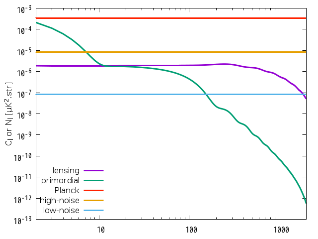
Figure 1: Noise sources assumed in Eq. (5) where we consider the cosmic variance (green), lensing effect of scalar perturbations (purple) and the white noise with $w_{p}^{-1/2}=1$ (cyan), $10$ (orange) and $63.1~{}\mu{\rm K}\cdot{\rm arcmin}$ (red), dubbed as “low-noise”, “high-noise” and “Planck” noise models, respectively.

Inverse of the Fisher matrix gives a covariance matrix of the reconstructed tensor power spectra. The diagonal elements give $1\sigma$ uncertainties of $\delta\mathcal{P}_{i}$ at each bin,

$$\sigma_{\delta\mathcal{P}_{i}}^{2}=(F^{-1})_{ii},.$$ (10)

III Results

Throughout this paper, we set $f_{\rm sky}=1$. In Fig. 2 we show $\sigma_{\delta\mathcal{P}_{i}}$ (Eq. 10) for $(r,n_{T},k_{0},k_{N},N,\alpha)=(0.01,0,10^{-4}~{}{\rm Mpc}^{-1},3\times 10^{-2}~{}{\rm Mpc}^{-1},8,2.04)$. The solid line shows the fiducial spectrum $\mathcal{P}^{\rm fid}_{h}$. Each box shows the $1\sigma$ region around the fiducial spectrum. On large scales, the uncertainty is mainly due to the cosmic variance. On small scales the contributions from noise and lensing dominate. The covariance matrix including off-diagonal terms is given in Table 2.

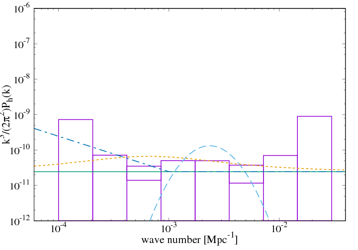
(a) “low-noise” : $(w_{p}^{-1/2},\lambda)=(1~{}\mu{\rm K}\cdot{\rm arcmin},1)$

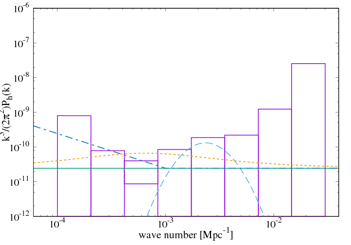
(b) “high-noise” : $(w_{p}^{-1/2},\lambda)=(10~{}\mu{\rm K}\cdot{\rm arcmin},1)$

(c) “delensed” : $(w_{p}^{-1/2},\lambda)=(1~{}\mu{\rm K}\cdot{\rm arcmin},0)$

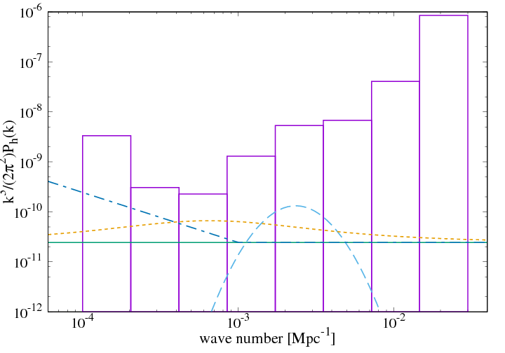
(d) “Planck” : $(w_{p}^{-1/2},\lambda)=(63.1~{}\mu{\rm K}\cdot{\rm arcmin},1)$

Figure 2: Uncertainty of the reconstructed tensor power spectrum from B-mode observations. The fiducial model has $r=0.01$ and $n_{T}=0$, and the reconstruction parameters are $k_{0}=10^{-4}~{}{\rm Mpc}^{-1}$, $k_{N}=3\times 10^{-2}~{}{\rm Mpc}^{-1}$, and $N=8$. (Top left) Low noise case. (Top right) High noise case. (Bottom left) Low noise with complete delensing. (Bottom right) Planck noise case. The solid line shows the fiducial spectrum, the dashed line an example spectrum from the SU(2)-axion model with $r_{*}=0.05$, $k_{p}=2.0\times 10^{-3}~{}{\rm Mpc}^{-1}$, and $\sigma=0.4$ Dimastrogiovanni:2016fuu , the dotted line a massive gravity inflation model with $(\alpha,\beta,N_{*},T_{\rm reh})=(0.7,1.0,47,10^{10}~{}{\rm GeV})$, and the dot-dashed line a red-tilted spectrum on large scales with $(k_{1},n_{T1})=(10^{-3}~{}{\rm Mpc}^{-1},-1.0)$.

	$\delta\mathcal{P}_{1}$	$\delta\mathcal{P}_{2}$	$\delta\mathcal{P}_{3}$	$\delta\mathcal{P}_{4}$	$\delta\mathcal{P}_{5}$	$\delta\mathcal{P}_{6}$	$\delta\mathcal{P}_{7}$	$\delta\mathcal{P}_{8}$
$\delta\mathcal{P}_{1}$	$4.9\times 10^{-19}$	$-3.0\times 10^{-20}$	$2.9\times 10^{-21}$	$-2.7\times 10^{-21}$	$2.6\times 10^{-22}$	$-2.8\times 10^{-23}$	$5.2\times 10^{-23}$	$-8.8\times 10^{-22}$
$\delta\mathcal{P}_{2}$	$-3.0\times 10^{-20}$	$2.2\times 10^{-21}$	$-2.5\times 10^{-22}$	$2.5\times 10^{-22}$	$-2.6\times 10^{-23}$	$3.1\times 10^{-24}$	$-5.6\times 10^{-24}$	$9.5\times 10^{-23}$
$\delta\mathcal{P}_{3}$	$2.9\times 10^{-21}$	$-2.5\times 10^{-22}$	$1.1\times 10^{-22}$	$-1.7\times 10^{-22}$	$2.7\times 10^{-23}$	$-3.5\times 10^{-24}$	$6.2\times 10^{-24}$	$-1.0\times 10^{-22}$
$\delta\mathcal{P}_{4}$	$-2.7\times 10^{-21}$	$2.5\times 10^{-22}$	$-1.7\times 10^{-22}$	$6.7\times 10^{-22}$	$-1.8\times 10^{-22}$	$2.5\times 10^{-23}$	$-4.2\times 10^{-23}$	$6.9\times 10^{-22}$
$\delta\mathcal{P}_{5}$	$2.6\times 10^{-22}$	$-2.6\times 10^{-23}$	$2.7\times 10^{-23}$	$-1.8\times 10^{-22}$	$6.5\times 10^{-22}$	$-1.8\times 10^{-22}$	$2.8\times 10^{-22}$	$-4.3\times 10^{-21}$
$\delta\mathcal{P}_{6}$	$-2.8\times 10^{-23}$	$3.1\times 10^{-24}$	$-3.5\times 10^{-24}$	$2.5\times 10^{-23}$	$-1.8\times 10^{-22}$	$1.7\times 10^{-22}$	$-4.8\times 10^{-22}$	$8.4\times 10^{-21}$
$\delta\mathcal{P}_{7}$	$5.2\times 10^{-23}$	$-5.6\times 10^{-24}$	$6.2\times 10^{-24}$	$-4.2\times 10^{-23}$	$2.8\times 10^{-22}$	$-4.8\times 10^{-22}$	$2.1\times 10^{-21}$	$-3.9\times 10^{-20}$
$\delta\mathcal{P}_{8}$	$-8.8\times 10^{-22}$	$9.5\times 10^{-23}$	$-1.0\times 10^{-22}$	$6.9\times 10^{-22}$	$-4.3\times 10^{-21}$	$8.4\times 10^{-21}$	$-3.9\times 10^{-20}$	$7.5\times 10^{-19}$

Table 2: Covariance matrix $(F^{-1})_{ij}$ for “low-noise” model with $N=8$ and $f_{\rm sky}=1$. The value enclosed in the boxes are the diagonal elements. The wavenumber of each bin is given by $k_{n}=\alpha^{n}k_{0}$ where $\alpha=(k_{N}/k_{0})^{1/N}=2.04$, and see Eq. (1). One can obtain the covariance matrix with $f_{\rm sky}<1$ by multiplying all the elements by $1/f_{\rm sky}$.

We find that the tensor power spectra are best reconstructed at two wavenumber bins around $k\approx 6\times 10^{-4}$ and $5\times 10^{-3}~{}{\rm Mpc}^{-1}$. While the precise wavenumbers at which the spectra are best constrained depend on the choice of bin sizes, we can understand these values analytically. The B-mode power spectrum of CMB polarization has two characteristic scales: the so-called “reionization bump” at $\ell\lesssim 6$ and the “recombinatiom bump” at $\ell\approx 80$. The wavenumber that gives the former is $k_{\rm reion}\approx 3/[r_{L}-r(z_{\rm reion})]$ Zaldarriaga:1996ke , where $r_{L}=14~{}{\rm Gpc}$ and $r(z_{\rm reion})\approx 9~{}{\rm Gpc}$ are the comoving distances to the surface of last scatter and the epoch of reionization, e.g., $z_{\rm reion}\approx 8$. We thus obtain $k_{\rm reion}\approx 6\times 10^{-4}~{}{\rm Mpc}^{-1}$. The wavenumber that gives the latter is $k_{\rm recomb}\approx 80/r_{L}\approx 6\times 10^{-3}~{}{\rm Mpc}^{-1}$.

Usually, the $1\sigma$ regions shrink as we go to higher wavenumbers where the number of modes is greater; however, we find in Fig. 2 an unusual feature that the $1\sigma$ regions shrink first, increase at $k\approx 10^{-3}~{}{\rm Mpc}^{-1}$, and shrink again at $k\gtrsim 2\times 10^{-3}~{}{\rm Mpc}^{-1}$. This is due to a gap (i.e., lack of the signal) between the reionization and recombination bumps. The transfer function leaves only a small B-mode signal here, making reconstruction of the initial tensor power spectrum noisy. With these we understand all the features in Fig. 2.

Can we distinguish between various models of the source of tensor modes from inflation? In Fig. 2 we show some theoretical predictions of the tensor power spectrum from an SU(2)-axion model with $(r_{*},k_{p},\sigma)=(0.05,2.0\times 10^{-3}~{}{\rm Mpc}^{-1},0.4)$, from a massive gravity inflation model with $(\alpha,\beta,T_{R},g_{*S},N_{*},n_{T*})=(0.7,1.0,10^{10}{\rm GeV},100,47,0)$ (see Appendix A), as well as from a red-tilted spectrum on large scales with $\mathcal{P}(k)=(k/k_{1})^{n_{T1}}$ for $k<k_{1}$ and $\mathcal{P}_{h}(k)=\mathcal{P}_{h}^{\rm fid}$ for $k\leq k_{1}$, which resembles predictions of an open inflation model associated with a bubble nucleation Yamauchi:2011qq . As an example, we show the spectrum with $(k_{1},n_{T1})=(10^{-3}~{}{\rm Mpc}^{-1},-1)$. We emphasize that these parameter choices are not at all robust predictions of the models, but serve only as examples.

To quantify how well we can distinguish models, we calculate the $\chi^{2}$ statistic including the off-diagonal elements of the full covariance matrix. To this end we calculate $\chi^{2}$ as

$$\chi^{2}=\sum_{i\leq j}^{N}\left[\mathcal{P}_{h}^{\rm fid}(k_{i})-\mathcal{P}_{h}^{\rm model}(k_{i})\right]F_{ij}\left[\mathcal{P}_{h}^{\rm fid}(k_{j})-\mathcal{P}_{h}^{\rm model}(k_{j})\right],$$ (11)

and the probability to exceed (PTE) defined as

$$P(\chi^{2}>a,N)=\int_{a}^{\infty}\!P(\chi^{2},N)\,d\chi^{2}.$$ (12)

Here, $P(x,n)$ is the $\chi^{2}$ distribution function for $n$ degrees of freedom,

$$P(x,N)=\frac{1}{2^{N/2}\Gamma(N/2)}x^{N/2-1}e^{-x/2}.$$ (13)

The PTE provides the probability to confuse the theoretically-predicted models mentioned above with the fiducial power spectrum. For simplicity, we fix the theoretical model parameters and do not include them in the degrees of freedom.

The values of $\chi^{2}$ and PTE with $N=8$ are tabulated in Table 3. For reference, we also compute them for the Planck observation with the corresponding white noise, $w_{p}^{-1/2}=63.1\mu{\rm K}\cdot{\rm arcmin}$, which is obtained by averaging the noise bandpowers in 70, 100, and 148 GHz Planck:2006aa . In the last row in Table 3, we also show $\chi^{2}$ for the null hypothesis, which is calculated by setting $\mathcal{P}_{h}^{\rm model}(k_{i})=0$ in Eq. (11). We find that Planck cannot detect the fiducial spectrum, and furthermore cannot distinguish the three theoretical predictions from it, since $\chi^{2}$ is of order unity and the corresponding PTE is also unity. On the other hand, the future observations with $w_{p}^{-1/2}=1~{}\mu$K$\cdot$arcmin can distinguish SU(2)-axion model and the massive gravity inflation model with high statistical significance, whereas the open inflation model is distinguished with moderate significance because of the cosmic variance at small wavenumbers.

One may be surprised that we can distinguish the models despite the fact that the error bars appear larger than the differences between some models and the fiducial spectrum in Fig. 2. This is due to large correlations between the bins (see Table 2). Indeed, ignoring the off-diagonal elements, i.e., $\sigma^{2}=\sum_{i}^{N}F_{ii}\left[\mathcal{P}_{h}^{\rm fid}(k_{i})-\mathcal{P}_{h}^{\rm model}(k_{i})\right]^{2}$, we find that, for $N\geq 8$ bins, $\sigma^{2}\ll\chi^{2}$. We also find that the values of $\sigma^{2}$ depend sensitively on the number of bins used, whereas those of $\chi^{2}$ with off-diagonal terms do not. Only when the size of the bins is sufficiently large (see $N=4$ in Table 4) $\chi^{2}$ and $\sigma^{2}$ agree because the bin-to-bin correlation would be suppressed in this case; thus, including the off-diagonal elements is essential.

So far, we have fixed the cosmological parameters. How would varying them change our results? Varying $\Omega_{M}$ and $H_{0}$ changes the distance to the last-scattering surface, shifting the B-mode power spectrum in the $\ell$ space. This would change the relationship between $k$ and $\ell$, shifting features in the reconstructed tensor power spectra in the $k$ space. Varying the optical depth $\tau$ changes the height of the reionization bump, which would affect the amplitude of the reconstructed power at $k=k_{\rm reion}\approx 6\times 10^{-4}~{}{\rm Mpc}^{-1}$. However, in the era when we can make precise measurements of the B-mode power spectrum, these parameters will be determined so precisely that their impacts would not be the dominant uncertainty in the reconstructed power spectra.

We have also fixed our fiducial tensor power spectrum at a power-law power spectrum with $n_{T}\approx 0$. This is because this spectrum is motivated by single-field slow-roll inflation models, and detecting difference from it would be a major discovery. Of course, we are free to use any spectra as the fiducial power spectrum.

	low-noise		high-noise		delensed		Planck
	$\chi^{2}$	PTE	$\chi^{2}$	PTE	$\chi^{2}$	PTE	$\chi^{2}$	PTE
SU(2)-axion	$1.5\times 10^{2}$	$9.3\times 10^{-28}$	$1.2\times 10^{1}$	$1.4\times 10^{-1}$	$6.3\times 10^{2}$	$1.6\times 10^{-131}$	$4.9\times 10^{-1}$	$1.0$
Massive	$1.2\times 10^{2}$	$1.4\times 10^{-21}$	$3.4\times 10^{1}$	$3.3\times 10^{-5}$	$3.6\times 10^{2}$	$7.7\times 10^{-73}$	$1.3$	$1.0$
Red-tilted	$2.0\times 10^{1}$	$1.1\times 10^{-2}$	$1.6\times 10^{1}$	$4.3\times 10^{-2}$	$2.1\times 10^{1}$	$6.0\times 10^{-3}$	$1.7$	$9.9\times 10^{-1}$
Null hypothesis	$3.1\times 10^{2}$	$1.1\times 10^{-61}$	$2.1\times 10^{1}$	$7.0\times 10^{-3}$	$1.4\times 10^{3}$	$9.0\times 10^{-295}$	$5.7\times 10^{-1}$	$1.0$

Table 3: $\chi^{2}$ and probability to exceed (PTE) for various noise models, ’low-noise’, ’high-noise’, ’delensed’ and ’Planck’, which corresponds to $(w_{p}^{-1/2},\lambda)=(1.0,1.0)$, $(10.0,1.0)$, $(1.0,0.0)$ and $(63.1,1.0)$, respectively.

	$\chi^{2}$				$\sigma^{2}$
	$N=4$	$N=8$	$N=12$	$N=16$	$N=4$	$N=8$	$N=12$	$N=16$
SU(2)-axion	2.2$\times 10^{3}$	$1.5\times 10^{2}$	$2.8\times 10^{2}$	$2.4\times 10^{2}$	$7.2\times 10^{2}$	$2.4\times 10^{1}$	$3.5\times 10^{1}$	$1.6\times 10^{1}$
Massive	1.4$\times 10^{2}$	$1.2\times 10^{2}$	$1.1\times 10^{2}$	$1.0\times 10^{2}$	$6.5\times 10^{1}$	$2.1\times 10^{1}$	$7.1$	$1.5$
Red-tilted	3.0$\times 10^{1}$	$2.0\times 10^{1}$	$1.6\times 10^{1}$	$1.5\times 10^{1}$	$2.5\times 10^{1}$	$4.2$	$5.5\times 10^{-1}$	$1.9\times 10^{-2}$
Null hypothesis	3.2$\times 10^{2}$	$3.1\times 10^{2}$	$2.8\times 10^{2}$	$2.7\times 10^{2}$	$7.5\times 10^{1}$	$1.1\times 10^{1}$	$4.6$	$1.9$

Table 4: Dependence of $\chi^{2}$ and $\sigma^{2}$ on the number of bins for “low-noise” model.

IV Conclusion

Reconstruction of the initial tensor power spectrum is complementary to the usual approach of forward-modeling (i.e., to calculate the B-mode CMB power spectrum from a given initial tensor power spectrum) because we can test various models of the early universe directly at the initial power spectrum level, without having to run Boltzmann solvers. In this paper we have calculated the covariance matrix of the reconstructed tensor power spectra in bins of wavenumbers. The $\chi^{2}$ statistic (Eq. 11) computed with this covariance matrix (given in Table 2 for the fiducial power spectrum with $r=0.01$ and $n_{T}=0$ and $1~{}\mu{\rm K}\cdot{\rm arcmin}$ noise) can be used to distinguish the tensor power spectra of one’s favorite early universe models from a power-law power spectrum. We find that reconstructed power spectra in bins of wavenumbers are highly correlated and thus including the off-diagonal elements in $\chi^{2}$ is essential in obtaining the correct answer.

We have tested our algorithm for three models, SU(2)-axion model Dimastrogiovanni:2016fuu , massive gravity inflation (Sec. A), and open inflation Yamauchi:2011qq , and find that future observations of CMB polarization by, e.g., LiteBIRD Matsumura:2013aja , should be able to distinguish the theoretical predictions of SU(2)-axion, open inflation, and massive gravity inflation models from a scale-invariant tensor power spectrum, depending on the model parameters. While we did not perform comprehensive parameter search for various models in this paper, we developed an interactive web tool to calculate $\chi^{2}$ for any parameter values specified by users. This application is available on-line at http://numerus.sakura.ne.jp/research/open/srec/srec.php. We describe this tool in Appendix B. The web tool returns the covariance matrix, the $\chi^{2}$ values and the PTE, and draws figures such as Fig. 2.

Appendix A Massive gravity inflation

We consider the inflationary massive gravity theory with the mass term that depends on dynamics of inflation.

$$m_{g}^{2}=f(\phi,\dot{\phi})\,.$$ (14)

Depending on the form of the function $f$, it may vary substantially during inflation.

The equation-of-motion for the tensor perturbation takes the form,

$$\ddot{\gamma}+3H\dot{\gamma}+\left(\frac{k^{2}}{a^{2}}+m_{g}^{2}\right)\gamma=0\,.$$ (15)

Assuming a very small slow-roll parameter $\epsilon=-\dot{H}/H^{2}$, we obtain

$$\frac{d^{2}\gamma}{dn^{2}}+3\frac{d\gamma}{dn}+\left(\frac{k^{2}}{a^{2}H^{2}}+\frac{m_{g}^{2}}{H^{2}}\right)\gamma=0\,,$$ (16)

where $dn=Hdt$. We set $n=n_{f}$ at the end of inflation. On superhorizon scales, assuming $m_{g}^{2}/H^{2}\ll 1$, the above equation is solved to give the amplitude at the end of inflation as

$$\gamma_{k}(n_{f})=\gamma_{k}(n_{k})\exp\left[-\int_{n_{k}}^{n_{f}}\frac{m_{g}^{2}}{3H^{2}}dn\right]\,,$$ (17)

where $n_{k}$ is the time at which the mode crosses the horizon, $k^{2}/a^{2}=H^{2}$, the rms amplitude of which is $\langle\gamma_{k}^{2}(n_{k})\rangle\propto H^{2}$ as usual. Thus the spectrum at the end of inflation is given by

$$P_{T}(k;n_{f}) \propto\exp\left[-\int_{n_{k}}^{n_{f}}\frac{2m_{g}^{2}}{3H^{2}}dn\right]\,,$$ (18)

where $n_{f}-n_{k}=\ln(k_{f}/k)$ and $k_{f}=a(n_{f})H$.

Now let us assume the time dependence of $m_{g}^{2}$ as

$$\frac{2m_{g}^{2}}{3H^{2}}=n_{T*}+\beta\alpha\frac{\sinh\alpha n}{\cosh^{2}\alpha n}\,,$$ (19)

where we assume $\alpha\lesssim 1$ but $\beta$ is arbitrary. We can then easily integrate it to find

$$\exp\left[-\int_{n_{k}}^{n_{f}}\frac{m_{g}^{2}}{3H^{2}}dn\right]=\exp\left[-n_{T*}N_{k}+\frac{\beta}{\cosh\alpha(N_{k}-N_{*})}-\frac{\beta}{\cosh\alpha N_{*}}\right]\,,$$ (20)

where $N_{k}=n_{f}-n_{k}=-\ln(k/k_{f})$ is the number of e-folds counted backward from the end of inflation, and $N_{*}=n_{f}$ is the time at which the feature in the spectrum appears. Since we assumed $\alpha\lesssim 1$ and we want $N_{*}$ to be fairly large $N_{*}\gtrsim 40-50$ to have an observable feature, the last term in the exponent is completely negligible. Thus we obtain

$$P_{T}(k;n_{f})\propto\exp\left[-n_{T*}N_{k}+\frac{\beta}{\cosh\alpha(N_{k}-N_{*})}\right]=\left(\frac{k}{k_{f}}\right)^{n_{T*}}\exp\left[\frac{\beta}{\cosh\alpha(N_{k}-N_{*})}\right]\,.$$ (21)

Thus the spectrum is the product of a power-law component and a factor peaked at $N=N_{*}$. The enhancement factor is $e^{\beta}$ relative to the baseline.

Appendix B User’s manual of ‘Spectrum Reconstructor’ 

We developed a web tool, ‘Spectrum Reconstructor’ , to compute the Fisher matrix of reconstructed initial tensor power spectra. In this section, we provide a brief instruction of this tool.

‘Spectrum Reconstructor’ assumes the cosmological parameters given in Table 1. It returns a Fisher matrix and a covariance matrix, and makes a plot of the fiducial power spectrum of tensor perturbations with error bars where the fiducial spectrum is assumed to be a power-low given in Eq. (2).

The covariance matrix is then used to compute $\chi^{2}$ and the PTE for various early universe models. Three kinds of model power spectra that are introduced in the main text are provided in the tool as ‘built-in models’. One can also upload numerical data of a power spectrum as ‘custom model’.

In the main page of the tool, we define the parameters controlling the Fisher analysis and plots, which are categorized into four tabs: ‘Basic’, ‘Drawing’, ‘Built-in models’ and ‘Custom models’. One can get information on each parameter in these tabs when one hovers over parameter names. In ‘Basic’ tab, one can specify the amplitude and the spectral index of the fiducial spectrum, the number of bins, and noise sources. In ‘Drawing’ tab, one can adjust the vertical and horizontal axes of the plot as well as the scale (logarithmic or linear). In ‘Built-in models’, one can set the model parameters of SU$(2)$-axion, open inflation, and the massive gravity models that are introduced in the main text, and also select the presence or absence of each model spectrum in the plot. Finally, in ‘Custom’ models, one can upload favorite power spectrum data in a simple text format.

After setting the parameters, clicking the ‘MAKE PLOT’ button generates a plot in the PNG format. If one selects the presence of some model spectra, the corresponding $\chi^{2}$’s and PTE’s are also tabulated below the plot. The Fisher and covariance matrices are provided in the text format at the link below the plot. This text file contains four blocks; the first two blocks are the Fisher matrices with and without the cosmic variance, and the remainings are the corresponding covariance matrices. The parameters and results including the uploaded spectrum, if exists, are preserved for a few days on the system.

Note that specifications and appearance of our web tool are subjected to change without prior notice for improvement.

References

- (1) U. Seljak and M. Zaldarriaga, Phys. Rev. Lett. 78 (1997) 2054 doi:10.1103/PhysRevLett.78.2054 [astro-ph/9609169].
- (2) M. Kamionkowski, A. Kosowsky and A. Stebbins, Phys. Rev. Lett. 78 (1997) 2058 doi:10.1103/PhysRevLett.78.2058 [astro-ph/9609132].
- (3) U. Seljak and M. Zaldarriaga, Astrophys. J. 469 (1996) 437 doi:10.1086/177793 [astro-ph/9603033].
- (4) A. Lewis, A. Challinor and A. Lasenby, Astrophys. J. 538 (2000) 473 doi:10.1086/309179 [astro-ph/9911177].
- (5) D. Blas, J. Lesgourgues and T. Tram, JCAP 1107 (2011) 034 doi:10.1088/1475-7516/2011/07/034 [arXiv:1104.2933 [astro-ph.CO]].
- (6) R. Brout, F. Englert and E. Gunzig, Annals Phys. 115, 78 (1978). doi:10.1016/0003-4916(78)90176-8
- (7) A. A. Starobinsky, Phys. Lett. 91B (1980) 99. doi:10.1016/0370-2693(80)90670-X
- (8) K. Sato, Mon. Not. Roy. Astron. Soc. 195 (1981) 467.
- (9) A. H. Guth, Phys. Rev. D 23 (1981) 347. doi:10.1103/PhysRevD.23.347
- (10) A. Albrecht and P. J. Steinhardt, Phys. Rev. Lett. 48 (1982) 1220. doi:10.1103/PhysRevLett.48.1220
- (11) A. D. Linde, Phys. Lett. 108B (1982) 389. doi:10.1016/0370-2693(82)91219-9
- (12) A. A. Starobinsky, JETP Lett. 30 (1979) 682 [Pisma Zh. Eksp. Teor. Fiz. 30 (1979) 719].
- (13) E. Dimastrogiovanni, M. Fasiello and T. Fujita, JCAP 1701 (2017) no.01, 019 doi:10.1088/1475-7516/2017/01/019 [arXiv:1608.04216 [astro-ph.CO]].
- (14) L. F. Abbott and M. B. Wise, Nucl. Phys. B 244 (1984) 541. doi:10.1016/0550-3213(84)90329-8
- (15) T. Tanaka and M. Sasaki, Prog. Theor. Phys. 97 (1997) 243 doi:10.1143/PTP.97.243 [astro-ph/9701053].
- (16) G. Domènech, T. Hiramatsu, C. Lin, M. Sasaki, M. Shiraishi and Y. Wang, JCAP 1705 (2017) no.05, 034 doi:10.1088/1475-7516/2017/05/034 [arXiv:1701.05554 [astro-ph.CO]].
- (17) T. Hiramatsu, R. Saito, A. Naruko and M. Sasaki, in preparation.
- (18) P. A. R. Ade et al. [Planck Collaboration], Astron. Astrophys. 594 (2016) A13 doi:10.1051/0004-6361/201525830 [arXiv:1502.01589 [astro-ph.CO]].
- (19) M. Zaldarriaga and U. Seljak, Phys. Rev. D 58, 023003 (1998) doi:10.1103/PhysRevD.58.023003 [astro-ph/9803150].
- (20) T. Namikawa and R. Nagata, JCAP 1510 (2015) no.10, 004 doi:10.1088/1475-7516/2015/10/004 [arXiv:1506.09209 [astro-ph.CO]].
- (21) A. Lewis and A. Challinor, Phys. Rept. 429 (2006) 1 doi:10.1016/j.physrep.2006.03.002 [astro-ph/0601594].
- (22) N. Katayama and E. Komatsu, Astrophys. J. 737 (2011) 78 doi:10.1088/0004-637X/737/2/78 [arXiv:1101.5210 [astro-ph.CO]].
- (23) B. Thorne, T. Fujita, M. Hazumi, N. Katayama, E. Komatsu and M. Shiraishi, Phys. Rev. D 97 (2018) no.4, 043506 doi:10.1103/PhysRevD.97.043506 [arXiv:1707.03240 [astro-ph.CO]].
- (24) T. Matsumura et al., J. Low. Temp. Phys. 176 (2014) 733 doi:10.1007/s10909-013-0996-1 [arXiv:1311.2847 [astro-ph.IM]].
- (25) M. Zaldarriaga, Phys. Rev. D 55, 1822 (1997) doi:10.1103/PhysRevD.55.1822 [astro-ph/9608050].
- (26) J. Tauber et al. [Planck Collaboration], astro-ph/0604069.
- (27) D. Yamauchi, A. Linde, A. Naruko, M. Sasaki and T. Tanaka, Phys. Rev. D 84 (2011) 043513 doi:10.1103/PhysRevD.84.043513 [arXiv:1105.2674 [hep-th]].