The generalized Brans-Dicke theory and its cosmology

Abstract

A generalized Brans-Dicke (GBD) theory is studied in this paper. The GBD theory is obtained by generalizing the Ricci scalar $R$ to an arbitrary function $f(R)$ in the original Brans-Dicke (BD) action. The interesting property has been found in the GBD theory, for example it can naturally solve the problem of $\gamma$ value emerging in $f(R)$ modified gravity (i.e. the inconsistent problem between the observational $\gamma$ value and the theoretical $\gamma$ value), without introducing the so-called chameleon mechanism. In this paper, we derive the cosmological equations and study the cosmology in the GBD theory. The cosmological solutions show that the GBD model can pass through the test of the observations, such as the observational Hubble data. Comparing with other theories, it can be found that the GBD theory have some other interesting properties or solve some problems existing in other theories. (1) It is well known that the $f(R)$ theory are equivalent to the BD theory with a potential (abbreviated as BDV) for taking a specific value of the BD parameter $\omega=0$, where the specific choice: $\omega=0$ for the BD parameter is quite exceptional, and it is hard to understand the corresponding absence of the kinetic term for the field. However, for the GBD theory, it is similar to the double scalar-fields model, and both fields in the GBD own the non-disappeared dynamical effect. (2) One knows that in the double scalar-fields quintom model, it is required to include both the canonical quintessence field and the non-canonical phantom field in order to make the state parameter to cross over $w=-1$, while several fundamental problems are associated with phantom field, such as the problem of negative kinetic term and the fine-tuning problem, etc. While, in the GBD model, the state parameter of geometrical dark energy can cross over the phantom boundary $w=-1$ as achieved in the quintom model, without bearing the problems existing in the quintom model. (3) The GBD theory tends to investigate the physics from the viewpoint of geometry, while the BDV or the two scalar-fields quintom model tends to solve physical problems from the viewpoint of matter. It is possible that several special characteristics of scalar fields could be revealed through studies of geometrical gravity in the GBD. As an example, we investigate the potential $V(\phi)$ of the BD scalar field, and an effective form of $V(\phi)$ could be given by studying on the GBD theory. And, it seems that a viable condition for the BD theory could be found, i.e. the BD parameter should be $\omega>0$ for $f>0$, if we assume that the effective form of the BD potential can be approximately written as a popular square function of $\phi$.

I Introduction

There are several observational and theoretical motivations to investigate the modified or alternative theories of general relativity. Studies on the modified gravity theories of GR have been always the hot area. Several modified gravity theories have been widely studied mg1 ; mg2 ; mg3 ; mg4 ; mg5 ; mg6 , especially two simple modifications to GR: the $f(R)$ theory fr-review1 ; fr-review2 and the Brans-Dicke (BD) theory original-BD .

Recent observations in Refs. VG-MNRAS-2004-dwarf ; VG-PRD-2004-white ; VG-APJ ; VG-PRD-2002-SN ; VG-PRL-1996-neutron indicate that the Newton gravitational constant $G$ maybe depends on time. Brans-Dicke (BD) theory is a popular one to describe the time-variable $G(t)$ gravity. As a simple theory in the scalar-tensor theories scalar-tensor , BD theory is apparently compatible with Mach’s principle mach-bd , and in which a scalar field $\phi$ can be introduced naturally by considering $\phi(t)\propto 1/G(t)$. But in the original BD theory original-BD , it is hard to interpret the cosmic acceleration indicated by the observations acceleration-98SN ; acceleration-99SN ; acceleration-WMAP . In order to obtain an accelerating universe, one usually modified this theory at three aspects: (1) introducing the invisible component—-dark energy in universe BD-DE , (2) assuming the coupling constant $\omega$ to be variable with respect to time BD-omegat1 ; BD-omegat2 , (3) adding a potential term to the original BD theory (abbreviate as BDV) BD-potential . The applications of these extended BD theories have been investigated widely, such as at the aspects of cosmology GBD-cosmic1 ; GBD-cosmic2 ; GBD-cosmic3 , weak-field approximation GBD-weak , observational constraints GBD-constraint1 ; GBD-constraint2 , and so on BD-widely1 ; BD-widely2 ; BD-widely3 .

In this paper, we investigate other way to explain the cosmic acceleration in the framework of the BD theory, i.e. we generalize the Ricci scalar $R$ to be an arbitrary function $f(R)$ in the original BD action (abbreviate as GBD), which is different from the studies on equivalence between the BD theory and the modified $f(R)$ theory mg6 . The interesting property has been found in the GBD model. For example, by using the method of the weak-field approximation Ref. GBD-L shows that the GBD theory can naturally solve the problem of $\gamma$ value emerging in $f(R)$ modified gravity (i.e. the inconsistent problem between the observational $\gamma$ value and the theoretical $\gamma$ value), without introducing the so-called chameleon mechanism. The chameleon mechanism is introduced to solve the problem of $\gamma$ value in the $f(R)$ modified gravity. Here $\gamma$ is the parametrized post-Newtonian (PPN) parameter.

The GBD cosmology is studied in this paper, and the structure of our paper is as follows. In section II, we briefly introduce the GBD theory, and derive to gain the field equations and the cosmological equations in the GBD theory. In section III, we give the cosmological solutions of the GBD model. It is shown that the GBD model can pass through the test of the observation, such as the observational Hubble data. In section IV and V, we investigate the properties of the geometrical dark energy and the effective potential of the BD scalar field in the GBD theory. By comparing with the preceding studies (such as the studies on the $f(R)$, the BDV, and the quintom models), some new ingredients and significant progresses of this work could be shown as follows. (1) In the GBD theory one can take an arbitrary value of $\omega$ and the kinetic-energy term of scalar field in the action is non-disappeared, which is obviously different from the $f(R)$ theory. The $f(R)$ gravity theory becomes equivalent to the BDV theory for a specific value of $\omega=0$ under a transformation, where the kinetic-energy term for the scalar field is absent. (2) The GBD theory tends to investigate the physics from the viewpoint of geometry, while the BDV tends to solve physical problems from the viewpoint of matter. Several special characteristics of scalar fields could be revealed through studies of geometrical gravity in the GBD, such as we can investigate to given an effective form of potential of the BD scalar field. (3) Comparing with the two scalar-fields quintom model, the effective state parameter of geometrical dark energy in the GBD model can cross over the phantom boundary: $w=-1$ without bearing the problems existing in the non-canonical phantom field. But, the phantom field is introduced in the double scalar-fields quintom model in order to cross over $w=-1$, where the puzzling problems are emergent, such as the negative kinetic term and the fine-tuning problem. Section VI is the conclusion.

II Field equations and cosmological equations in the GBD theory

In framework of the time-variable gravitational constant, we study a generalized Brans-Dicke theory by using a function $f(R)$ to replace the Ricci scalar $R$ in the original BD action. The action of system is written as

$$S=S_{g}(g_{\mu\nu},\phi)+S_{m}(g_{\mu\nu},\psi)=\frac{1}{2}\int d^{4}x{\cal L}_{T},$$ (1)

with the total Lagrange quantity ${\cal L}_{T}$

$${\cal L}_{T}={\cal L}_{g}+{\cal L}_{\phi}+{\cal L}_{m}=\sqrt{-g}[\phi f(R)-\frac{\omega}{2\phi}\partial_{\mu}\phi\partial^{\mu}\phi+\frac{16\pi}{c^{4}}L_{m}].$$ (2)

Obviously, the system contains three dynamical variable: the gravitational field $g_{\mu\nu}$, the matter field $\psi$ and the BD scalar field $\phi$. $\omega$ is the couple constant. According to Eq. (2), it is easy to see that the GBD theory can be considered as a special case of the more general $f(R,\phi)$ theory fR-phi ; fR-phi1 ; fR-phi2 . It is well known that the so-called $f(\phi)R$ theory fphiR ; fphiR1 , as a special case of the $f(R,\phi)$ theory, has been widely studied fphiR2 ; fphiR3 ; fphiR4 . Given that $f(R,\phi)$ is a more complex theory and the more simple theory is usually more favored by the researcher in physics, here we investigate the GBD model induced by the directly observational motivation of the accelerating universe and some other motivations exhibited in the introduction. Concretely, we discuss some interesting cosmological contents in the GBD model, such as the comparison with observation, the properties of effective state parameter for the geometrical dark energy, the effective potential of the BD scalar field, etc.

Taking $c=1$ and varying the action with respect to metric $\frac{\delta S}{\delta g^{\mu\nu}}=\frac{\delta S_{g}(g_{\mu\nu},\phi)}{\delta g^{\mu\nu}}+\frac{\delta S_{m}(g_{\mu\nu},\psi)}{\delta g^{\mu\nu}}=0$, one can get the gravitational field equation

$$\phi\left[f_{R}R_{\mu\nu}-\frac{1}{2}f(R)g_{\mu\nu}\right]-(\nabla_{\mu}\nabla_{\nu}-g_{\mu\nu}\Box)(\phi f_{R})+\frac{1}{2}\frac{\omega}{\phi}g_{\mu\nu}\partial_{\sigma}\phi\partial^{\sigma}\phi-\frac{\omega}{\phi}\partial_{\mu}\phi\partial_{\nu}\phi=8\pi T_{\mu\nu},$$ (3)

where $f_{R}\equiv\partial f/\partial R$, $\nabla_{\mu}$ is the covariant derivative associated with the Levi-Civita connection of the metric, $\Box\equiv\nabla^{\mu}\nabla_{\mu}$, and $T_{\mu\nu}=\frac{-2}{\sqrt{-g}}\frac{\delta S_{m}}{\delta g^{\mu\nu}}$ is the energy momentum tensor of the matter. Varying the action (1) with respect to the scalar field $\phi$ and the matter field $\psi$ give respectively

$$f(R)+2\omega\frac{\Box\phi}{\phi}-\frac{\omega}{\phi^{2}}\partial_{\mu}\phi\partial^{\mu}\phi=0,$$ (4)

$$\frac{\delta S}{\delta\psi}=\frac{\delta S_{g}(g_{\mu\nu},\phi)}{\delta\psi}+\frac{\delta S_{m}(g_{\mu\nu},\psi)}{\delta\psi}=0.$$ (5)

The trace of Eq. (3) is

$$f_{R}R-2f(R)+\frac{3\Box(\phi f_{R})}{\phi}+\frac{\omega}{\phi^{2}}\partial_{\mu}\phi\partial^{\mu}\phi=\frac{8\pi T}{\phi}.$$ (6)

From Eqs. (4) and (6), one can see that the curvature of the spacetime could be caused by the motion of $\phi$. And from Eq. (3), it is shown that the BD scalar field does not exert any direct influence on matter, while it couples with another scalar field $f_{R}$. Furthermore, the standard $f(R)$ modified gravity is recovered for $\phi$=constant, while above equations reduce to the Einstein’s general relativity (GR) for both BD scalar field $\phi$=constant and $f(R)=R$. Combining Eqs. (4) and (6), we get

$$\Box\phi-\frac{\partial_{\mu}\phi\partial^{\mu}\phi}{4\phi}=\frac{1}{4\omega}[8\pi T-\phi Rf_{R}-3\Box(\phi f_{R})].$$ (7)

One can read from Eq. (7) that, for $\omega\rightarrow\infty$ the constant-$G$ theory can be recovered, which is same to the result in the standard BD theory.

In the flat Friedmann-Lemaitre-Robertson-Walker (FLRW) metric

$$ds^{2}=-dt^{2}+a^{2}\left(t\right)d\vec{x}^{2},$$ (8)

using Eqs. (3) and (4), we can derive the evolutional equations of the background universe in the GBD theory,

$$3f_{R}H^{2}=\frac{8\pi\rho_{m}}{\phi}+\frac{f_{R}R-f(R)}{2}-3H\dot{f_{R}}+\frac{1}{2}\omega\left(\frac{\dot{\phi}}{\phi}\right)^{2}-3Hf_{R}\frac{\dot{\phi}}{\phi},$$ (9)

$$-2f_{R}\dot{H}=\frac{8\pi}{\phi}(\rho_{m}+p_{m})+\ddot{f_{R}}-H\dot{f_{R}}+\omega\left(\frac{\dot{\phi}}{\phi}\right)^{2}-Hf_{R}\frac{\dot{\phi}}{\phi}+f_{R}\frac{\ddot{\phi}}{\phi}+2\frac{\dot{\phi}}{\phi}\dot{f_{R}},$$ (10)

$$f(R)-\omega\left(\frac{\dot{\phi}}{\phi}\right)^{2}+2\omega\frac{\stackrel{{\scriptstyle\cdot\cdot}}{{\phi}}}{\phi}+6\omega H\frac{\dot{\phi}}{\phi}=0.$$ (11)

Here $a$ is the cosmic scale factor, $H$ is the Hubble parameter, $R=6\left(2H^{2}+\stackrel{{\scriptstyle\cdot}}{{H}}\right)$, and ”dot” denotes the derivative with respect to cosmic time $t$. For case of $\phi$=constant ($\dot{\phi}=0$ and $\ddot{\phi}=0$) in Eqs.(9-11), they are reduced to the $f(R)$ theory, while for case of $f(R)=R$ they are reduced to the original Brans-Dicke theory.

III Cosmological solutions in the GBD theory

For solving the cosmological equations (9-11), we define the dimensionless variables:

$$y_{H}=H^{2}/m^{2}-a^{-3},$$ (12)

$$y_{R}=R/m^{2}-3a^{-3},$$ (13)

$$y_{\phi}=\phi/\phi_{0},$$ (14)

$$y_{\phi}^{{}^{\prime}}=\phi^{{}^{\prime}}/\phi_{0},$$ (15)

Thus using Eqs. (9) and (11), we get the differential equations for $\{y_{H},y_{R},y_{\phi},y_{\phi}^{{}^{\prime}}\}$ as follows

$$y_{H}^{{}^{\prime}}=\frac{1}{3}y_{R}-4y_{H},$$ (16)

$$y_{R}^{{}^{\prime}}=\frac{-[(y_{H}+a^{-3})f_{R}-\frac{f_{R}}{6}(y_{R}+3a^{-3})+\frac{f}{6m^{2}}-\frac{\omega}{6}(\frac{y_{\phi}^{{}^{\prime}}}{y_{\phi}})^{2}(y_{H}+a^{-3})+f_{R}\frac{y_{\phi}^{{}^{\prime}}}{y_{\phi}}(y_{H}+a^{-3})-\frac{a^{-3}}{\phi}]}{(y_{H}+a^{-3})m^{2}f_{RR}}+9a^{-3},$$ (17)

$$y_{\phi}^{{}^{\prime}}=\phi^{{}^{\prime}}/\phi_{0},$$ (18)

$$y_{\phi}^{{}^{\prime\prime}}=\frac{\phi}{2\omega(y_{H}+a^{-3})}[\frac{-f}{m^{2}}+\omega(\frac{y_{\phi}^{{}^{\prime}}}{y_{\phi}})^{2}(y_{H}+a^{-3})-\omega\frac{y_{\phi}^{{}^{\prime}}}{y_{\phi}}(\frac{1}{3}y_{R}-4y_{H}-3a^{-3})-6\omega\frac{y_{\phi}^{{}^{\prime}}}{y_{\phi}}(y_{H}+a^{-3})].$$ (19)

Here the subscript ”0” denotes the current value of parameters, the superscript ^′ denotes the derivative with respect to $\ln a$, the parameter $m$ is defined as $m^{2}=(8315Mpc)^{-2}(\frac{\Omega_{0m}h^{2}}{0.13})$ and $\Omega_{0m}$ is the current dimensionless energy density of the matter. To solve above differential equations, the initial conditions ($a_{0}=1$) are expressed respectively as

$$y_{H}|_{a=1}=H_{0}^{2}/m^{2}-1,$$ (20)

$$y_{R}|_{a=1}=6H_{0}^{2}(1-q_{0})/m^{2}-3,$$ (21)

$$y_{\phi}|_{a=1}=1,$$ (22)

$$y_{\phi}^{{}^{\prime}}|_{a=1}=0.01.$$ (23)

Here $q=-\frac{\ddot{a}}{aH^{2}}$ is the deceleration parameter, and its current value $q_{0}$ can be given by the cosmic observations. The value of the initial condition $y_{\phi}^{{}^{\prime}}|_{a=1}$ can be indicated by the following observations. For example, the limits on the variation of $G$ can be exhibited by: $|\frac{\dot{G}}{G}|=|\frac{\dot{\phi}}{\phi}|\leq 4.1\times 10^{-10}y^{-1}$ from Pulsating white dwarf G117-B15A VG-MNRAS-2004-dwarf , $-4\times 10^{-11}y^{-1}\leq\frac{\dot{\phi}}{\phi}\leq 2.5\times 10^{-10}y^{-1}$ from Nonradial pulsations of white dwarfs VG-PRD-2004-white , $|\frac{\dot{\phi}}{\phi}|\leq 2.3\times 10^{-11}y^{-1}$ from Millisecond pulsar PSR J0437-4715 VG-APJ , $|\frac{\dot{\phi}}{\phi}|\leq 10^{-11}y^{-1}$ from Type-Ia supernovae VG-PRD-2002-SN , $\frac{\dot{\phi}}{\phi}=(0.6\pm 4.2)\times 10^{-12}y^{-1}$ from Neutron star masses VG-PRL-1996-neutron , $|\frac{\dot{\phi}}{\phi}|\leq 1.6\times 10^{-12}y^{-1}$ from Helioseismology vg-constraint6 , and $\frac{\dot{\phi}}{\phi}=(4\pm 9)\times 10^{-13}y^{-1}$ from Lunar laser ranging experiment vg-constraint7 , etc. Taking a stringent bound $|\frac{\dot{\phi}}{\phi}|\leq 10^{-12}y^{-1}$ and considering the current value of the dimensionless Hubble constant $h=0.673\pm 0.010$ from the Planck 2015 results hubble-value , we can calculate to limit $|y_{\phi}^{{}^{\prime}}({a=1})|\leq 0.015$ by using the center value $H_{0}=67.3kms^{-1}Mpc^{-1}=6.87\times 10^{-11}y^{-1}$. Here we take $y_{\phi}^{{}^{\prime}}({a=1})=0.01$ as an initial condition in Eq. (23). For comparison, the cases of other initial values of $y_{\phi}^{{}^{\prime}}({a=1})$ (less than 0.01) are also discussed.

To find a cosmological solution of the GBD theory, we need to take a concrete form of $f(R)$ function at prior. As an example, we consider an interesting model called exponential gravity

$$f(R)=R-\beta R_{s}(1-e^{-R/R_{s}}),$$ (24)

which is proposed by Refs.viable-fr-e1 ; viable-fr-e2 ; viable-fr-e3 . Here $\beta$ and $R_{s}$ are two constants with $\beta R_{s}\simeq 12H_{0}^{2}\Omega_{0m}$ viable-fr-e3 . This model has an important feature that it has only one more parameter than the $\Lambda$CDM model. The first and the second derivatives of Eq. (24) with respect to $R$ are

$$f_{R}=1-\beta e^{-R/R_{s}},$$ (25)

$$f_{RR}=\frac{\beta}{R_{s}}e^{-R/R_{s}}.$$ (26)

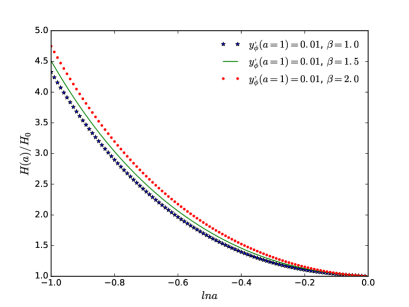
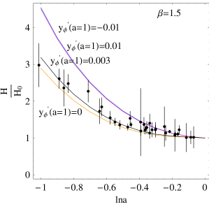
Figure 1: The numerical solutions of $H(a)/H_{0}$ in the GBD model with the different model parameter $\beta$ or the different initial condition $y_{\phi}^{{}^{\prime}}(a_{0})$.

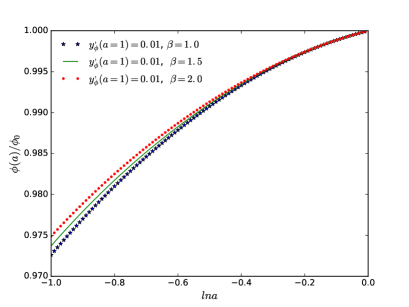
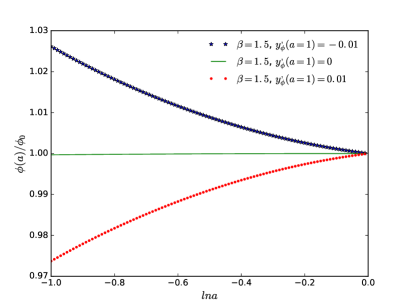
Figure 2: The numerical solutions of $\phi(a)/\phi_{0}$ in the GBD model with the different model parameter $\beta$ or the different initial condition $y_{\phi}^{{}^{\prime}}(a_{0})$.

Thus using the system of the ordinary differential equations (16)-(19) and the initial conditions (20)-(23), we can numerically exhibit the solutions: $H(a)$ and $\phi(a)$ in the GBD theory, which are illustrated in Fig.1 and Fig.2.

In Fig.1 (left), we show the dependence of $H(a)$ on the parameter $\beta$. Fig.1 (right) illustrates the evolution of $H(a)$ with respect to $\ln a$ with taking the different values of $y_{\phi}^{{}^{\prime}}(a=1)$. In the following, we use $a_{0}$ to denotes the current value: $a=1$. We can see that the evolutions of $H(a)$ almost have the same trajectory for two cases: $y_{\phi}^{{}^{\prime}}(a_{0})=0.01$ and $y_{\phi}^{{}^{\prime}}(a_{0})=-0.01$, while the evolutions of $H(a)$ are obviously different for two cases: $y_{\phi}^{{}^{\prime}}(a_{0})=0.01$ and $y_{\phi}^{{}^{\prime}}(a_{0})=0$. It seems that the effect to $H(a)$ from the BD field is notable. Using the observational Hubble data listed in table 1, we display these observational $H(z)$ value in Fig.1 (right). Here $z=(1-a)/a$ is the cosmic redshift. It is shown from Fig.1 (right) that the most observational $H(z)$ data are located in the region between the case of $y_{\phi}^{{}^{\prime}}(a_{0})=0$ and the case of $y_{\phi}^{{}^{\prime}}(a_{0})=\pm 0.01$. It seems that the GBD model could pass through the test of the observation, such as the observational Hubble data, since the evolution of $H(a)$ with $y_{\phi}^{{}^{\prime}}(a_{0})=0.003$ is well consistent with those observational data. From Fig.2 (right), one can see that evolutional tendency of BD scalar field depends on the initial value of $y_{\phi}^{{}^{\prime}}(a_{0})$.

z	0.0708	0.09	0.12	0.17	0.179	0.199	0.20	0.24	0.27
H(z)	$69.0\pm 19.68$	$69.0\pm 12.0$	$68.6\pm 26.2$	$83.0\pm 8.0$	$75.0\pm 4.0$	$75.0\pm 5.0$	$72.9\pm 29.6$	$79.69\pm 2.65$	$77.0\pm 14.0$
Ref.	ohd-13	ohd-14	ohd-13	ohd-15	ohd-16	ohd-16	ohd-13	ohd-17	ohd-15
z	0.28	0.35	0.352	0.3802	0.4	0.4004	0.4247	0.43	0.44
H(z)	$88.8\pm 36.6$	$84.4\pm 7.0$	$83.0\pm 14.0$	$83.0\pm 13.5$	$95.0\pm 17.0$	$77.0\pm 10.2$	$87.1\pm 11.2$	$86.45\pm 3.68$	$82.6\pm 7.8$
Ref.	ohd-13	ohd-18	ohd-16	ohd-19	ohd-15	ohd-19	ohd-19	ohd-17	ohd-20
z	0.4497	0.4783	0.48	0.57	0.593	0.6	0.68	0.73	0.781
H(z)	$92.8\pm 12.9$	$80.9\pm 9.0$	$97.0\pm 62.0$	$92.4\pm 4.5$	$104.0\pm 13.0$	$87.9\pm 6.1$	$92.0\pm 8.0$	$97.3\pm 7.0$	$105.0\pm 12.0$
Ref.	ohd-19	ohd-19	ohd-21	ohd-22	ohd-16	ohd-20	ohd-16	ohd-20	ohd-16
z	0.875	0.9	1.037	1.3	1.363	1.43	1.75
H(z)	$125.0\pm 17.0$	$117.0\pm 23.0$	$154.0\pm 20.0$	$168.0\pm 17.0$	$160.0\pm 33.6$	$177.0\pm 18.0$	$202.0\pm 40.0$
Ref.	ohd-16	ohd-15	ohd-16	ohd-15	ohd-23	ohd-15	ohd-15

Table 1: The values of Hubble parameter given by observations.

IV Effective state parameter of geometrical dark energy in the GBD

Probing properties of the dark energy is important, and it has been studied in the standard cosmology or the several modified gravity theories DE ; DE1 ; DE2 ; DE3 ; DE4 ; DE5 ; DE6 ; DE7 ; DE8 ; DE9 ; DE10 ; DE11 ; multi-field ; multi-field1 ; multi-field2 ; DE-lu1 ; DE-lu2 . Next we investigate the properties of geometrical dark energy in this GBD theory, and analyze the effects of the BD scalar field. Rewriting the Eq.(3) as follows

$$G_{\mu\nu} = R_{\mu\nu}-\frac{1}{2}Rg_{\mu\nu}=\frac{8\pi T_{\mu\nu}^{eff}}{\phi_{0}},$$ (27)

with

$$T_{\mu\nu}^{eff}=\frac{\phi_{0}}{\phi}\frac{T_{\mu\nu}}{f_{R}}$$

$$+\frac{\phi_{0}}{8\pi f_{R}}[(\nabla_{\mu}\nabla_{\nu}-g_{\mu\nu}\Box)f_{R}+\frac{1}{2}f(R)g_{\mu\nu}-\frac{1}{2}f_{R}Rg_{\mu\nu}+\frac{f_{R}}{\phi}(\nabla_{\mu}\nabla_{\nu}-g_{\mu\nu}\Box)\phi$$

$$-\frac{1}{2}\frac{\omega}{\phi^{2}}g_{\mu\nu}\partial_{\sigma}\phi\partial^{\sigma}\phi+\frac{\omega}{\phi^{2}}\partial_{\mu}\phi\partial_{\nu}\phi],$$ (28)

then the effective energy density and the effective pressure are derived as

$$\rho^{eff}=\frac{\phi_{0}}{\phi}\frac{\rho_{m}}{f_{R}}+\frac{\phi_{0}}{8\pi f_{R}}\left[-3H\dot{f_{R}}-\frac{1}{2}f(R)+\frac{1}{2}f_{R}R-3Hf_{R}\frac{\dot{\phi}}{\phi}+\frac{1}{2}\omega(\frac{\dot{\phi}}{\phi})^{2}\right]$$ (29)

$$p^{eff}=\frac{\phi_{0}}{\phi}\frac{p_{m}}{f_{R}}+\frac{\phi_{0}}{8\pi f_{R}}\left[\ddot{f_{R}}+2H\dot{f_{R}}+\frac{1}{2}f(R)-\frac{1}{2}f_{R}R+f_{R}\frac{\ddot{\phi}}{\phi}+2Hf_{R}\frac{\dot{\phi}}{\phi}+\frac{1}{2}\omega(\frac{\dot{\phi}}{\phi})^{2}+2\frac{\dot{\phi}}{\phi}\dot{f_{R}}\right].$$ (30)

Here $\rho_{m}$ and $p_{m}$ are the energy density and the pressure of matter, respectively. According to Eqs. (27) and (28), we can define the effective Newton gravitational constant $G_{eff}=\frac{1}{\phi f_{R}}$. To keep the attractive property of gravity, we get an constraint: $\phi f_{R}>0$. If we assume $\phi>0$, then $f_{R}>0$. The effective state parameter for geometrical dark energy has a form

$$w^{eff}_{g}=\frac{p^{eff}-p_{m}}{\rho^{eff}_{g}-\rho_{m}}=\frac{8\pi\phi_{0}p_{m}-8\pi\phi p_{m}f_{R}+\phi_{0}\phi\left[\ddot{f_{R}}+2H\dot{f_{R}}+\frac{1}{2}f(R)-\frac{1}{2}f_{R}R+f_{R}\frac{\ddot{\phi}}{\phi}+2Hf_{R}\frac{\dot{\phi}}{\phi}+\frac{1}{2}\omega(\frac{\dot{\phi}}{\phi})^{2}+2\frac{\dot{\phi}}{\phi}\dot{f_{R}}\right]}{8\pi\phi_{0}\rho_{m}-8\pi\phi\rho_{m}f_{R}+\phi_{0}\phi\left[-3H\dot{f_{R}}-\frac{1}{2}f(R)+\frac{1}{2}f_{R}R-3Hf_{R}\frac{\dot{\phi}}{\phi}+\frac{1}{2}\omega(\frac{\dot{\phi}}{\phi})^{2}\right]}.$$ (31)

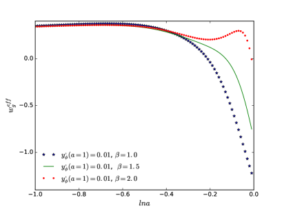
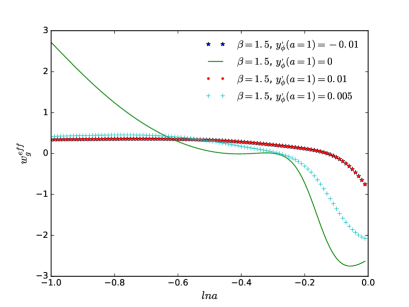
Figure 3: The evolutions of $w_{g}^{eff}(a)$ in the GBD model with the different model parameter $\beta$ or the different initial condition $y_{\phi}^{{}^{\prime}}(a_{0})$.

Taking the function $f(R)=R+\beta R_{s}(1-e^{-R/R_{s}})$ as an example, we plot the evolution of $w^{eff}_{g}(a)$ in Fig.3 by using the different values of model parameter $\beta$ and the initial values $y_{\phi}^{{}^{\prime}}(a_{0})$. In this GBD model, the dependence of $w^{eff}_{g}(a)$ on the model parameter $\beta$ are illustrated in Fig.3 (left). In the Fig.3 (right), one can see that $w^{eff}_{g}(a)$ almost have the same evolutions for the two cases: $y_{\phi}^{{}^{\prime}}(a_{0})=\pm 0.01$, i.e. the trajectories of $w^{eff}_{g}(a)$ are not sensitive to the symbol of initial condition $y_{\phi}^{{}^{\prime}}(a_{0})$, while the effect on $w^{eff}_{g}(a)$ from the BD scalar field is notable since the evolution of $w^{eff}_{g}(a)$ with $y_{\phi}^{{}^{\prime}}(a_{0})=0$ is obviously different from other three cases: $y_{\phi}^{{}^{\prime}}(a_{0})=\pm 0.01$ and $y_{\phi}^{{}^{\prime}}(a_{0})=0.005$. Also, one can see that the current value $w^{0eff}_{g}$ with $y_{\phi}^{{}^{\prime}}(a_{0})=0$ has the more small value than other cases of $y_{\phi}^{{}^{\prime}}(a_{0})\neq 0$, while $w^{eff}_{g}(a)$ with $y_{\phi}^{{}^{\prime}}(a_{0})=0$ has the more large value than the cases of $y_{\phi}^{{}^{\prime}}(a_{0})\neq 0$ at the high redshift $\ln a=-1$. And the values of $w^{0eff}_{g}$ are located in the range [-2.63,-0.75] for using the different initial conditions: from $y_{\phi}^{{}^{\prime}}(a_{0})=0$ to $y_{\phi}^{{}^{\prime}}(a_{0})=\pm 0.01$. The evolutions of $w^{eff}_{g}(a)$ with $y_{\phi}^{{}^{\prime}}(a_{0})=\pm 0.01$ in Fig.3 show that they vary from $w\sim\frac{1}{3}$ (radiation) to $w<0$ (dark energy).

It is shown in Eqs.(4) and (6) that the GBD model can be equivalently considered as the two scalar-fields model. It can be found in Fig.3 that the effective state parameter of geometrical dark energy in the GBD model can cross over the phantom boundary, as achieved in the double scalar-fields quintom model quintom-feng . But we can notice that it is required to include both the canonical quintessence field and the non-canonical phantom field in the double scalar-fields quintom model quintom-feng , in order to make the state parameter to cross over the phantom boundary: $w=-1$, where several fundamental problems are associated with phantom field, such as the problem of negative kinetic term and the fine-tuning problem, etc. It is shown that the GBD model can paly a role of the quintom without bearing the problems existing in the two-fields quintom model, which is also a motivation to appeal us to study the GBD model.

V A effective potential of the BD scalar field in the GBD theory

One knows that the potential of a scalar field usually paly an important role in the early inflation universe and the late accelerating universe. Determining the forms of the potential function for a scalar field is significative, since the potential display some properties for a scalar field. By using Eqs. (4) and (6), the equations of motion for the Brans-Dicke scalar field $\phi$ and the other scalar field $\varphi=f_{R}$ are expressed as follows

$$\Box\phi=\frac{\partial_{\mu}\phi\partial^{\mu}\phi}{2\phi}-\frac{\phi f}{2\omega}=-V_{\phi}(\phi),$$ (32)

$$\Box f_{R}=\frac{1}{3}[\frac{8\pi T}{\phi}-f_{R}R+2f-3f_{R}\frac{\Box\phi}{\phi}-6\dot{f_{R}}\frac{\dot{\phi}}{\phi}-\frac{\omega\partial_{\mu}\phi\partial^{\mu}\phi}{\phi^{2}}]=-\mathcal{V}_{\varphi}(\varphi)+\frac{8\pi T}{3\phi}.$$ (33)

Obviously, this GBD theory is similar to the two scalar-fields theory. Here $V(\phi)$ and $\mathcal{V}(\varphi)$ denotes the effective potential of fields, and the subscript $\phi$ (or $\varphi$) denotes the derivative with respect to scalar field. The effective forms of $V_{\phi}$ and $\mathcal{V}_{\varphi}$ can be gained by comparing with the standard form of equation of motion for the canonical scalar field, i.e. the standard Klein-Gordon equation in the vacuum: $\Box\Phi+V_{\Phi}(\Phi)=0$.

One knows that the geometrical representation may be more appealing to relativists due to its more apparent geometrical nature, whereas the scalar-field representation seems more appealing to particle physicists. Obviously, the GBD theory tends to investigate the physics from the viewpoint of geometry, while the BDV tends to solve physical problems from the viewpoint of matter. Given that the equivalence between the BDV theory and the $f(R)$ theory, some properties of the BD scalar field could be found. So, it is possible that several special characteristics of scalar fields could be revealed through studies of geometrical gravity in the GBD. Next we investigate the effective form of potential $V(\phi)$ of the BD scalar field $\phi$. Assuming that the variable $\phi$ is independent of its derivative $\partial_{\mu}\phi$ and the geometrical quantity $f(R)$, we can gain an effective form of $V(\phi)$ by integrating Eq.(32) with respect to $\phi$

$$V(\phi)=\frac{H^{2}\phi^{{}^{\prime}2}}{2}\ln\phi+\frac{f}{4\omega}\phi^{2}+C(\dot{\phi},f).$$ (34)

Here superscript ^′ denotes the derivative with respect to $\ln a$, $C$ is a parameter that is independent of $\phi$. Using Eq.(34) and taking $C=0$, we can plot the shapes of BD effective potential in Fig.4. We can see from Fig.4 that the trajectories of BD effective potential $V(\phi)$ are not sensitive to the variation of $\beta$ values, while the shapes of $V(\phi)$ much depend on the initial condition $y_{\phi}^{{}^{\prime}}(a_{0})$ for the smaller $\ln a$ ($\ln a<-0.4$), and for $\ln a>-0.4$ one has $V(\phi)\sim 0$. Obviously, C$(\dot{\phi},f)$ in Eq. (34) is a undetermined freedom, whose uncertainty can be used to modify the trajectories of the BD effective potential.

Furthermore, an interesting property can be found in the GBD theory by comparing with $f(R)$ theory. It is well known that, the $f(R)$ theory are equivalent to the BDV theory with taking a specific value of the BD parameter $\omega=0$ fr-bd2 ; fr-bd3 . However, the specific choice: $\omega=0$ for the BD parameter is quite exceptional, and it is hard to understand the corresponding absence of the kinetic-energy term for the scalar field. But in the GBD theory, one can read from Eq.(2) that the value of $\omega$ is arbitrary and the kinetic-energy term of the scalar field is non-disappeared. In addition, if we assume that the effective form of the BD potential can be approximately written as a popular square function of $\phi$, i.e. we assume $V(\phi)\simeq V_{0}+\frac{1}{2}m^{2}\phi^{2}$ bd-potential1 ; bd-potential2 , then we have $V_{\phi}\simeq m^{2}\phi$ with $m$ owning the mass dimension. Thus, we need to require $\dot{\phi}^{2}\simeq 0$ (i.e. a slow-rolling field) in Eq. (32), and then we gain $m^{2}=\frac{f}{2\omega}$. Obviously, if $f>0$, we get an constraint on the BD parameter $\omega>0$. And $\omega$ should own a large value with the requirement of a small value of $m^{2}$.

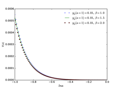
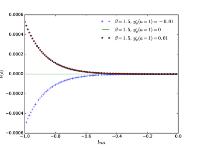
Figure 4: The evolutions of effective potential for Brans-Dicke scalar field with the different model parameter $\beta$ and the different initial condition $y_{\phi}^{{}^{\prime}}(a_{0})$.

VI Conclusion

The GBD theory is investigated in this paper, which is obtained by generalizing the Ricci scalar $R$ to an arbitrary function $f(R)$ in the original Brans-Dicke action. This theory can be reduced to the original BD theory and the $f(R)$ modified gravity under certain conditions. We give the gravitational field equation and the BD scalar-field equation in the GBD theory. Using the FLRW metric and the field equations, we can obtain the cosmological equations in this theory. The evolutional equations of universe and BD field are numerically solved by taking a concrete form of $f(R)$ function. It is shown that the modification to $H(a)$ from the dynamical BD scalar field is notable, and the GBD model can pass through the test of the observation, such as the observational Hubble data.

The trajectories of the effective state parameter for the geometrical dark energy is studied in the GBD universe, which indicates that the evolutions of $w^{eff}_{g}(a)$ with $y_{\phi}^{{}^{\prime}}(a_{0})\neq 0$ can vary from radiation ($w^{eff}_{g}\sim 1/3$) to dark energy ($w^{eff}_{g}<0$). And the modifications to the state parameter from the BD scalar field is remarkable. In addition, the effective potential of Brans-Dicke field is investigated in the GBD model. One can see that the evolutions of the BD effective potential depend on the initial value of $y_{\phi}^{{}^{\prime}}(a_{0})$, especially they are sensitive to the given symbol of $y_{\phi}^{{}^{\prime}}(a_{0})$.

Ref. GBD-L shows an interesting property of the GBD theory, where the GBD theory can naturally solve the problem of $\gamma$ value emerging in $f(R)$ modified gravity (i.e. the inconsistent problem between the observational $\gamma$ (PPN parameter) value and the theoretical $\gamma$ value), without introducing the so-called chameleon mechanism. In this paper, we also compare our results with other theories. It can be seen that the GBD theory have some other interesting properties or solve some problems existing in other theories. (1) We can notice that it is required to include both the canonical quintessence field and the non-canonical phantom field in the double scalar-fields quintom model, in order to make the state parameter to cross over the phantom boundary: $w=-1$, while several fundamental problems are associated with the non-canonical phantom field, such as the problem of negative kinetic term and the fine-tuning problem, etc. It can be found that in this paper the effective state parameter of geometrical dark energy in the GBD model can cross over the phantom boundary without bearing the problems relating with the phantom field. (2) It is well known that, the $f(R)$ theory are equivalent to the BDV theory with a specific value of the BD parameter $\omega=0$. However, the specific choice: $\omega=0$ for the BD parameter is quite exceptional, and it is hard to understand the corresponding absence of the kinetic term for the scalar field in the action of the BDV theory, while in the GBD theory the value of $\omega$ is arbitrary and the dynamical effect of the scalar field is non-disappeared. (3) One knows that the geometrical representation may be more appealing to relativists due to its more apparent geometrical nature, whereas the scalar-field representation seems more appealing to particle physicists. Obviously, the GBD theory tends to investigate the physics from the viewpoint of geometry, while the BDV or the quintom scalar-field model tends to solve physical problems from the viewpoint of matter. Given that the equivalence between the BDV theory and the $f(R)$ theory, some properties of the BD scalar field could be found. So, it is possible that several special characteristics of scalar fields could be revealed through studies of geometrical gravity in the GBD. As shown in this paper, an effective form of the BD potential can be gained by studying the GBD theory. And, it seems that a viable condition for the BD theory could be found, i.e. the BD parameter should be $\omega>0$ for $f>0$, if we assume that the effective form of the BD potential can be approximately written as a popular square function of $\phi$.

Acknowledgments The research work is supported by the National Natural Science Foundation of China (11645003,11705079,11575075,11475143).

References

- (1) J. Lu, G. Chee, JHEP 05, 024 (2016).
- (2) Q.G. Huang, Eur. Phys. J. C (2014) 74, 2964 [arXiv:1403.0655].
- (3) M. Hohmann, L. Jarv, P. Kuusk, E. Randla, O. Vilson, Phys. Rev. D 94, 124015 (2016) [arXiv:1607.02356].
- (4) S. Nojiri, S.D. Odintsov, V.K. Oikonomou, Phys.Rept. 692 (2017) 1-104 [arXiv:1705.11098].
- (5) A. de la Cruz-Dombriz, E. Elizalde, S. D. Odintsov, D. Saez-Gomez, JCAP 05, 060 (2016) [arXiv:1603.05537].
- (6) T. P. Sotiriou, Class. Quant. Grav. 23, 5117 (2006).
- (7) A. De Felice, S. Tsujikawa, Living Rev. Relativity, 13, 3, (2010).
- (8) T. P. Sotiriou, V. Faraoni, Rev. Mod. Phys. 82:451-497, 2010 [arXiv:0805.1726].
- (9) C. Brans, R.H. Dicke, Phys. Rev. 124, 925 (1961).
- (10) M. Biesiada and B. Malec, Mon. Not. Roy. Astron. Soc. 350, 644 (2004) [astro-ph/0303489].
- (11) O. G. Benvenuto et al., Phys. Rev. D, 69, 082002, (2004).
- (12) J.P.W. Verbiest et al., Astrophys. J. 679, 675 (2008) [arXiv:0801.2589].
- (13) E. Gaztanaga, et al, Phys. Rev. D 65, 023506, 2002 [arXiv:astro-ph/0109299].
- (14) S. E. Thorsett, Phys. Rev. Lett. 77, 1432 (1996) [astro-ph/9607003].
- (15) K. Bamba, D. Momeni, R. Myrzakulov, Int.J.Geom.Meth.Mod.Phys. 12(10), 1550106 (2015) [arXiv:1404.4255]
- (16) L. Qiang, Y. Ma, M. Han, D. Yu, Phys. Rev. D 71, 061501 (2005).
- (17) A.G. Riess et al., Astron. J. 116, 1009 (1998).
- (18) S. Perlmutter et al., Astrophys. J. 517, 565 (1999).
- (19) D.N. Spergel et al., Astrophys. J. Suppl. 148, 175 (2003).
- (20) L.X. Xu, W.B Li, J.B. Lu, Eur. Phys. J. C 60, 135 (2009).
- (21) N. Banerjee, D. Pavon, Phys. Rev. D 63, 043504 (2001).
- (22) A.D. Felice, S. Tsujikawa, JCAP 07, 024 (2010).
- (23) J. Lu, S. Gao, Y. Zhao and Y. Wu, Eur. Phys. J. Plus 127, 154 (2012).
- (24) N. Roy, N. Banerjee, Phys. Rev. D 95, 064048 (2017) [arXiv:1702.02169].
- (25) L.X. Xu, W.B Li, J.B. Lu, Eur. Phys. J. C 60, 135 (2009).
- (26) O. Hrycyna, M. Szydlowski, JCAP 12 (2013) 016 [arXiv:1310.1961].
- (27) H. Ozer, O. Delice, Class. Quantum Grav. 35 (2018) 065002 [arXiv:1708.05900].
- (28) R. C. Freitas, S.V.B. Goncalves, Physics Letters B 703 (2011) 209-216 [arXiv:1111.5045].
- (29) X. Zhang, J. Yu, T. Liu, W. Zhao, A. Wang, Phys. Rev. D 95, 124008 (2017) [arXiv:1703.09853].
- (30) S. K. Tripathy, D. Behera, B. Mishra, Eur. Phys. J . C. (2015) 75:149 [arXiv:1410.3156].
- (31) G. Papagiannopoulos, J. D. Barrow, S. Basilakos, A. Giacomini, A. Paliathanasis, Phys. Rev. D 95, 024021 (2017) [arXiv:1611.00667].
- (32) M. Sharif, Rubab Manzoor, Eur. Phys. J. C 76 (2016) 330 [arXiv:1606.00758].
- (33) J. Lu, Y. Wang, X. Zhao, Phys. Lett. B, 795 (2019) 129 C134 [arXiv:1904.01734].
- (34) J.C. Hwang, Class. Quantum Grav. 7, 1613-1631 (1990).
- (35) J.C. Hwang, H. Noh, Phys. Rev. D 54, 1460 (1996).
- (36) J.C. Hwang, H. Noh, Phys. Rev. D 71, 063536 (2005).
- (37) S.D. Odintsov, V.K. Oikonomou, Nuclear Physics B 929, 79-112 (2018) [arXiv:1801.10529].
- (38) Y. Huang, Y. Gong, D. Liang, Z. Yi, Eur. Phys. J. C 75, 351 (2015) [arXiv:1504.01271].
- (39) B. Boisseau, Phys.Rev.D 83:043521 (2011) [arXiv:1011.2915].
- (40) B. Boisseau, H. Giacomini, D. Polarski, A. A. Starobinsky, JCAP 07, 002 (2015) [arXiv:1504.07927].
- (41) T. Chiba, M. Yamaguchi, JCAP 10, 040 (2013) [arXiv:1308.1142].
- (42) D.B. Guenther, L.M. Krauss, P. Demarque, Astrophys. J. 498, 871 (1998).
- (43) J.G. Williams, S.G. Turyshev, D.H. Boggs, Phys. Rev. Lett. 93, 261101 (2004), [arXiv:gr-qc/0411113].
- (44) A.G. Riess et al., Astrophys. J. 699, 539 (2009) [arXiv:0905.0695].
- (45) P. Zhang, M. Liguori, R. Bean, S. Dodelson, Phys.Rev.Lett. 99, 141302 (2007) [arXiv:0704.1932].
- (46) E.V. Linder, Phys.Rev.D 80, 123528 (2009) [arXiv:0905.2962].
- (47) K. Bamba, C.G. Geng, C.C. Lee, JCAP 08, 021 (2010) [arXiv:1005.4574].
- (48) C. Zhang, H. Zhang, S. Yuan, S. Liu, T.J. Zhang and Y.C. Sun, Research in Astronomy and Astrophysics 14 (2014) 1221-1233, [arXiv:1207.4541].
- (49) R. Jimenez, L. Verde, T. Treu and D. Stern, Astrophys. J. 593 (2003) 622-629, [arXiv:0302560].
- (50) J. Simon, L. Verde and R. Jimenez, Gravit. Cosmol. 71 (2005) 123001, [arXiv:0412269].
- (51) M. Moresco, L. Verde, L. Pozzetti, R. Jimenez and A. Cimatti, JCAP (2012) 53, [arXiv:1201.6658].
- (52) E. Gaztanaga, A. Cabrse and L. Hui, [arXiv:0807.3551].
- (53) X. Xu, A. J. Cuesta, N. Padmanabhan, D. J. Eisenstein and C. K. McBride, Mon. Not. R. Astron. Soc. 431 (2013) 2834-2860, [arXiv:1206.6732].
- (54) M. Moresco, L. Pozzetti and A. Cimatti et al., JCAP 5 (2016) 014, [arXiv:1601.01701].
- (55) C. Blake, S. Brough and M. Colless, et al., Mon. Not. R. Astron. Soc. 425 (2012) 405-414, [arXiv:1204.3674].
- (56) D. Stern, R. Jimenez and L. Verde, et al., J. Cosmol. Astropart. Phys. 2 (2010) 8, [arXiv:0907.3149].
- (57) L. Samushia, B. A. Reid and M. White, et al., Mon. Not. R. Astron. Soc. 429 (2013) 1514-1528, [arXiv:1206.5309].
- (58) M. Moresco, Mon. Not. R. Astron. Soc. Lett. 450 (2015) L16-L20, [arXiv:1503.01116].
- (59) R.G. Cai, S.J. Wang, Phys. Rev. D 93, 023515 (2016) [arXiv:1511.00627].
- (60) J.J. Guo, J.F. Zhang, Y.H. Li, D.Z. He, X. Zhang, Sci. China-Phys. Mech. Astron. 61, 030011 (2018) [arXiv:1710.03068].
- (61) T. Yang, Z.K. Guo, R.G. Cai, Phys. Rev. D 91, 123533 (2015) [arXiv:1505.04443].
- (62) H. Wei, X.B. Zou, H.Y. Li, D.Z. Xue, Eur. Phys. J. C 77 (2017) 14 [arXiv:1605.04571].
- (63) Q.G. Huang, Eur. Phys. J. C (2014) 74, 2964 [arXiv:1403.0655].
- (64) Y. Fan, P.X. Wu, H.W. Yu, Physical Review D 92, 083529 (2015) [arXiv:1510.04010].
- (65) X. Zhang, Sci. China-Phys. Mech. Astron. 60, 060431 (2017) [arXiv:1703.00651].
- (66) L.X. Xu, Phys. Rev. D.87, 043503(2013) [arXiv:1210.7413].
- (67) S. Li, Y.G. Ma, Eur.Phys.J.C 68, 227-239 (2010) [arXiv:1004.4350].
- (68) L. Feng, J.F. Zhang, X. Zhang, Sci. China-Phys. Mech. Astron. 61, 050411 (2018) [arXiv:1706.06913].
- (69) L.X. Xu, Phys. Rev. D.87, 043525(2013) [arXiv:1302.2291].
- (70) J.B. Lu, G.Y. Chee, JHEP 05, 024 (2016).
- (71) M. Hohmann, L. Jarv, P. Kuusk, E. Randla, O. Vilson, Phys. Rev. D 94, 124015 (2016) [arXiv:1607.02356].
- (72) S. Nojiri, S.D. Odintsov, V.K. Oikonomou, Phys.Rept. 692 (2017) 1-104 [arXiv:1705.11098].
- (73) A. de la Cruz-Dombriz, E. Elizalde, S. D. Odintsov, D. Saez-Gomez, JCAP 05, 060 (2016) [arXiv:1603.05537].
- (74) J. Lu, D. Geng, L. Xu, Y. Wu, M. Liu, JHEP 02, 071 (2015) [arXiv:1312.0779].
- (75) J. Lu, M. Liu, Y. Wu, Y. Wang, W. Yang, Eur. Phys. J. C 76, 679 (2016) [arXiv:1606.02987].
- (76) B.Feng, X.L. Wang, X.M. Zhang, Phys. Lett., B 607, 35-41 (2005) [arXiv:astro-ph/0404224]
- (77) S. Capozziello and M. De Laurentis, Phys. Rept. 509, 167 (2011).
- (78) S. Nojiri, S. D. Odintsov, and V. K. Oikonomou, Phys. Rep. 692, 1 (2017).
- (79) S. Capozziello, C. Corda, M. F. De Laurentis, Phys.Lett.B 669:255-259, 2008 [arXiv:0812.2272].
- (80) C. Corda, Eur.Phys.J.C 65:257-267,2010 [arXiv:1007.4077].