Two-qubit causal structures and the geometry of positive qubit-maps

Abstract

We study quantum causal inference in a set-up proposed by Ried et al. [Nat. Phys. 11, 414 (2015)] in which a common-cause scenario can be mixed with a cause-effect scenario, and for which it was found that quantum mechanics can bring an advantage in distinguishing the two scenarios: Whereas in classical statistics, interventions such as randomized trials are needed, a quantum observational scheme can be enough to detect the causal structure if the common cause results from a maximally entangled state.
We analyze this setup in terms of the geometry of unital positive but not completely positive qubit-maps, arising from the mixture of qubit-channels and steering maps. We find the range of mixing parameters that can generate given correlations, and prove a quantum advantage in a more general setup, allowing arbitrary unital channels and initial states with fully mixed reduced states. This is achieved by establishing new bounds on signed singular values of sums of matrices. Based on the geometry, we quantify and identify the origin of the quantum advantage depending on the observed correlations, and discuss how additional constraints can lead to a unique solution of the problem.

I Introduction

Imagine a scenario where two experimenters, Alice and Bob, sit in two distinct laboratories. At one point Alice opens the door of her laboratory, obtains a coin, checks whether it shows heads or tails and puts it back out of the laboratory. Some time later also Bob obtains a coin and also he checks whether it shows heads or tails. This experiment is repeated many times (ideally: infinitely many times) and after this they meet and analyze their joint outcomes. Assuming their joint probability distribution entails correlations, there must be some underlying causal mechanism which causally connects their coins Reichenbach (1971). This could be an unobserved confounder (acting as a common-cause), and they actually measured two distinct coins influenced by the confounder. Or it could be that Alice’s coin was propagated by some mechanism to Bob’s laboratory, and hence they actually measured the same coin, with the consequence that manipulations of the coin by Alice can directly influence Bob’s result (cause-effect scenario). The task of Alice and Bob is to determine the underlying causal structure, i.e. to distinguish the two scenarios. This would be rather easy if Alice could prepare her coin after the observation by her choice and then check whether this influences the joint probability (so-called “interventionist scheme”). In the present scenario, however, we assume that this is not allowed (so-called “observational scheme”). All that Alice and Bob have are therefore the given correlations, and from those alone, in general they cannot solve this task without additional assumptions. Ried et al. Ried et al. (2015) showed that in a similar quantum scenario involving qubits the above task can actually be accomplished in certain cases even in an observational scheme (see below for a discussion of how the idea of an observational scheme can be generalized to quantum mechanics).

In the present work we consider the same setup as in Ried et al. (2015), and allow arbitrary convex combinations of the two scenarios: The common-cause scenario is realized with probability $p$, the cause-effect scenario with probability $1-p$. Our main result are statements about the ranges of the parameter $p$ for which observed correlations can be explained with either one of the scenarios, or both. For this, we cast the problem in the language of affine representations of unital positive qubit maps Bengtsson and Życzkowski (2006) in which all the information is encoded in a $3\times 3$ real matrix, as is standard in quantum information theory for completely positive unital qubit maps Nielsen and Chuang (2010).

The paper is structured as follows: In section II we introduce causal models for classical random variables and for quantum systems. Therein we define what we consider a quantum observational scheme. Section III introduces the mathematical framework of ellipsoidal representations of qubit quantum-channels and qubit steering-maps. In section IV we define our problem mathematically and prove the main results, which we then comment in the last section V.

II Causal inference: classical versus quantum

II.1 Classical causal inference

At the heart of a classical causal model is a set of random variables $X_{1},X_{2},...,X_{N}$. The observation of a specific value of a variable, $X_{i}=x_{i}$, is associated with an event. Correlations between events hint at some kind of causal mechanism that links the events Reichenbach (1971) . Such a mechanism can be a deterministic law as for example $x_{i}=f(x_{j})$ or can be a probabilistic process described by conditional probabilities $P(x_{i}|x_{j})$, i.e. the probability to find $X_{i}=x_{i}$ given $X_{j}=x_{j}$ was observed. The causal mechanism may not be merely a direct causal influence from one observed event on the other, but may be due to common causes that lead with a certain probability to both events — or a mixture between both scenarios. Hence, by merely analysing correlations $P(x_{1},x_{2},\ldots,x_{n})$, i.e. the joint probability distribution of all events, one can, in general, without prior knowledge of the data generating process, not uniquely determine the causal mechanism that leads to the observed correlations (purely observational scheme). To remedy this, an intervention is often necessary, where the value of a variable $X_{i}$ whose causal influence one wants to investigate, is set by an experimentalist to different values, trying to see whether this changes the statistics of the remaining events (interventionist scheme). One strategy for reducing the influence of other, unknown factors, is to randomize the samples. This is for example a typical approach in clinical studies, where one group of randomly selected probands receives a treatment whose efficiency one wants to investigate, and a randomly selected control group receives a placebo. If the percentage of cured people in the first group is significantly larger than in the second group, one can believe in a positive causal effect of the treatment. The probabilities obtained in this interventionist scheme are so-called “do-probabilities” (or “causal conditional probabilities”) Pearl (2009): $P\left(x_{i}|\text{do}(x_{j})\right)$ is the probability to find $X_{i}=x_{i}$ if an experimentalist intervened and set the value of $X_{j}$ to the value $x_{j}$. This is different from $P\left(x_{i}|x_{j}\right)$, as a possible causal influence from some other unknown event on $X_{j}=x_{j}$ is cut, i.e. one deliberately modifies the underlying causal structure for better understanding a part of it. If $X_{j}=x_{j}$ was the only direct cause of $X_{i}=x_{i}$ then $P\left(x_{i}|x_{j}\right)=P\left(x_{i}|\text{do}(x_{j})\right)$. If instead the event $X_{i}=x_{i}$ was a cause of $X_{j}=x_{j}$, then intervening on $X_{j}$ cannot change $X_{i}$: $P(x_{i})=P\left(x_{i}|\text{do}(x_{j})\right)=P\left(x_{i}|\text{do}(\bar{x_{j}})\right)$, where $\bar{x_{j}}$ is a value different from $x_{j}$. If the correlation between $X_{i}=x_{i}$ and $X_{j}=x_{j}$ is purely because of a common cause, then no intervenion on $X_{i}$ or $X_{j}$ will change the probability to find a given value of the other: $P(x_{i})=P\left(x_{i}|\text{do}(x_{j})\right)$ for all $x_{j}$, and $P(x_{j})=P\left(x_{j}|\text{do}(x_{i})\right)$ for all $x_{i}$. Observing these do-probabilities one can hence draw conclusions about the causal influences behind the correlations observed in the occurence of $X_{i}=x_{i}$ and $X_{j}=x_{j}$.

In practice, direct causation in one direction is often excluded by time-ordering and need not to be investigated. For example, when doubting that one can conclude that smoking causes lung cancer from the observed correlations between these two events, it does not make sense to claim that having lung cancer causes smoking, as usually smoking comes before developing lung cancer. But even dividing a large number of people randomly into two groups and forcing one of them to smoke and the other not to smoke in order to find out if there is a common cause for both would be ethically inacceptable. The needed do-probabilities can therefore not always be obtained by experiment. Interestingly, the causal-probability calculus allows one in certain cases, depending notably on the graph structure, to calculate do-probabilities from observed correlations without having to do the intervention. Inversely, apart from only predicting the conditional probabilities for a random variable say $X_{i}$ given the observation of $X_{j}=x_{j}$, denoted as $P(x_{i}|x_{j})$, a causal model can also predict the do-probabilities, i.e. the distribution of $X_{i}$ if one would intervene on the variable $X_{j}$ and set its value to $x_{j}$. This is crucial for deriving informed recommendations for actions targeted at modifying certain probabilities, e.g. recommending not to smoke in order to reduce the risk for cancer.

The structure of a causal model can be depicted by a graph. Each random variable is represented by a vertex of the graph. Causal connections are represented by directed arrows and imply that signaling along the direction of the arrow is possible. In a classical causal model it is assumed that events happen at specific points in space and time, therefore bidirectional signaling is not possible as it would imply signaling backward in time. Hence the graph cannot contain cycles and is therefore a directed acyclic graph (DAG) Pearl (2009), see FIG.1. The set of parents $PA_{j}$ of the random variable $X_{j}$ is defined as the set of all variables that have an immediate arrow pointing towards $X_{j}$, and $pa_{j}$ denotes a possible value of $PA_{j}$. The causal model is then defined through its graph with random variables $X_{i}$ at its vertices and the weights $P(x_{j}|pa_{j})$ of each edge, i.e. the probabilities that $X_{j}=x_{j}$ happens under the condition that $Pa_{j}=pa_{j}$ occurred. The model generates the entire correlation function according to

$$P(x_{1},\ldots,x_{n})=\prod_{j=1}^{n}P(x_{j}|pa_{j})\,,$$ (1)

which is referred to as causal Markov condition Pearl (2009). When all $P(x_{1},\ldots,x_{n})$ are given, then all conditional probabilities follow, hence all $P(x_{j}|pa_{j})$ that appear in a given graph, but in general not all correlations nor all $P(x_{j}|pa_{j})$ are known (see below). The causal inference probleme consists in finding a graph structure that allows one to satisfy eq.(1) for given data $P(x_{1},\ldots,x_{n})$ and all known $P(x_{j}|pa_{j})$, where the unknown $P(x_{j}|pa_{j})$ can be considered fit-parameters in case of incomplete data. With access to the full joint probability distribution, the causal inference only needs to determine the graph. In practice, however, one often has only incomplete data: as long as a common cause has not been determined yet, one will not have data involving correlations of the corresponding variable. For example, one may have strong correlations between getting lung cancer (random variable $X_{2}\in\{0,1\}$) and smoking (random variable $X_{1}\in\{0,1\}$), but if there is a unknown common cause $X_{0}$ for both, one typically has no information about $P(x_{0},x_{1},x_{2})$: One will only start collecting data about correlations between the presence of a certain gene, say, and the habit of smoking or developing lung cancer once one suspects that gene to be a cause for at least one of these. In this case $P(x_{1}|x_{0})$ and $P(x_{2}|x_{0})$ are fit parameters to the model as well. The possibility of extending a causal model through inclusion of unknown random variables is one reason why in general there is no unique solution to the causal inference problem based on correlations alone. Interventions on $X_{i}$ make it possible, on the other hand, to cut $X_{i}$ from its parents and hence eliminate unknown causes one by one for all random variables.

Once a causal model is known, one can calculate all distributions

$$P(x_{1},...,x_{n}|i_{1},...,i_{n}) =\prod_{j=1}^{n}P(x_{j}|pa_{j},i_{j}),$$ (2)

for all possible combinations of interventions and observations, where the $i_{j}$ are the values of the intervention variable $I_{j}$ for the event $X_{j}$, $i_{j}=\text{idle}$ or $i_{j}=\text{do}(x_{j})$. Here, $P\left(x_{j}|pa_{j},i_{j}=\text{do}(\tilde{x}_{j})\right)=\delta_{x_{j},\tilde{x}_{j}}$ reflects that an intervention on $X_{j}$ deterministically sets its value, independently of the observed values of its causal parents. If $I_{j}=\text{idle}$ then the value of $X_{j}$ only depends on its causal parents $PA_{j}$, i.e. $P(x_{j}|\{x_{i}\}_{i\neq j},i_{j}=\text{idle})=P(x_{j}|pa_{j},i_{j}=\text{idle})$.

Figure 1: Simple DAG in a four party scenario. The parental structure is $\text{PA}_{A}=\{\},\;\text{PA}_{B}=\{A\},\;\text{PA}_{C}=\{A,B\},\;\text{PA}_{D}=\{C\}$. According to the causal Markov condition, eq. (2), the probability distribution then factorizes as ${P(a,b,c,d|i_{A},i_{B},i_{C},i_{D})=P(d|c,i_{D})P(c|a,b,i_{C})P(b|a,i_{B})P(a|i_{A})}$.

The field of causal discovery or causal inference aims at providing methods to determine the causal model, that is the DAG and the joint-probability distributions entering (1) for a given scenario. Different combinations of the $I_{j}$ correspond to different strategies. If all the interventions are set to idle, and hence all the outcomes are determined by the causal parents, one has the purely observational approach. In multivariate scenarios, where more than two random variables are involved, the observation of the joint probability distribution alone can still contain hints of the causal structure based on conditional independencies Pearl (2009). Nevertheless, in the bivariate scenario, i.e. when only two random variables are involved, classical correlations obtained by observations do not comprise any causal information. Only if assumptions for example on the noise distribution are taken a priori, information on the causal model can be obtained from observational data Mooij et al. (2016).

II.2 Quantum causal inference

The notion of causal models does not easily translate to quantum mechanics. The main problem is that in quantum systems not all observables can have predefined values independent of observation. Similiar to an operational formulation of quantum mechanics Chiribella et al. (2011), the process matrix formalism was introduced Oreshkov et al. (2012) and a quantum version of an event defined. In Costa and Shrapnel (2016) this is reviewed for the purpose of causal models. In place of the random variables in the classical case there are local laboratories. Within a process each laboratory obtains a quantum system as input and produces a quantum system as output. A quantum event corresponds to information which is obtained within a laboratory and is associated with a completely positive (CP) map mapping the input Hilbert space to the output Hilbert space of the laboratory. The possible events depend on the choice of instrument. An instrument is a set of CP maps that sum to a completely positive trace preserving (CPTP) map. For example an instrument can be a projective measurement in a specific basis, with the events the possible outcomes. The possibility to choose different instruments mirrors the possibility of interventions in the classical case (Costa and Shrapnel, 2016, 3.3). The whole information about mechanisms, which are represented as CPTP maps, and the causal connections is contained in a so-called process matrix. Besides its analogy for a classical causal model, the process framework goes beyond classical causal structures as it does not assume such a fixed causal structure Oreshkov et al. (2012). This recently stirred a lot of research Oreshkov and Giarmatzi (2016); Procopio et al. (2015); Chiribella (2012); Guérin et al. (2016). For a more detailed introduction we refer the reader especially to reference Costa and Shrapnel (2016) where a comprehensive description is provided.

The analogue of causal inference in the classical case is the reconstruction of a process matrix. This can be done using informationally complete sets of instruments, theoretically described in (Costa and Shrapnel, 2016, 4.1) and experimentally implemented in Ried et al. (2015). Defining a quantum observational scheme in analogy to the classical one is not straight forward. In general a quantum measurement destroys much of the states’ character and hence can almost never be considered a passive observation. For example if the system was initially in a pure state $|\psi\rangle$ but one measures in a basis such that $|\psi\rangle$ is not an eigenstate of the projectors onto the basis states, then the measurement truly changes the state of the system and the original state is not reproduced in the statistical average. In (Costa and Shrapnel, 2016, sect. 5) an observational scheme is simply defined as projective measurements in a fixed basis, in particular without assumptions about the incoming state of a laboratory and thus without assumptions about the underlying process. Another possibility to define an observational scheme is based on the idea that in the classical world observations reveal pre-existing properties of physical systems and that quantum observations should reproduce this. As a consequence, if one mixes the post-measurement states with the probabilities of the corresponding measurement outcomes, one should obtain the same state as before the measurement. That is ensured if and only if operations that do not destroy the quantum character of the state are allowed, as coherences cannot be restored by averaging. Ried et al. Ried et al. (2015) formalized this notion as “informational symmetry”, but considered only preservation of local states. For the special case of locally completely mixed states, they showed that projective measurements in arbitrary bases possess informational symmetry. This definition of a quantum observational scheme is problematic due to two reasons: Firstly, the allowed class of instruments depends on the incoming state, i.e. one can only apply projective measurements that are diagonal in the same basis as the state itself. This is at variance with the typical motivation for an observational scheme, namely that the instruments are restricted a-priori due to practical reasons. Moreoever, having measurements depend on the state requires prior knowledge about the state of the system, but finding out the state of the system is part of the causal inference (e.g.: are the correlations based on a state shared by Alice and Bob?). Hence, in general one cannot assume sufficient knowledge of the state for restricting the measurements such that they do not destroy coherences.
Secondly, the definition is unnaturally restrictive as it only considers the local state and not the global state. For example if Alice and Bob share a singlet state $|\psi\rangle=\frac{|01\rangle-|10\rangle}{\sqrt{2}}$, then both local states are completely mixed. Hence according to the informational symmetry, they are allowed to perform projective measurements in arbitrary bases. If Alice and Bob now both measure in the computational basis, they will each obtain both outcomes with probability $1/2$ and their local states will remain invariant in the statistical average $\rho_{A}^{\prime}=\rho_{A}=\frac{\mathbb{1}}{2}=\rho_{B}^{\prime}=\rho_{B}$. However, the global state does not remain intact. The post-measurement state is given as $\rho_{AB}^{\prime}=\frac{1}{2}\left(|01\rangle\langle 01|+|10\rangle\langle 10|\right)$ which is not even entangled anymore. But even defining a “global informational symmetry”, i.e. requiring the global state to remain invariant, does not settle the issue in a convenient way, as this would not allow any local measurements of Alice and Bob.

Here we propose three different schemes ranging from full quantum interventions over a quantum-observational scheme with the possibility of an active choice of measurements, to a passive quantum observational scheme in a fixed basis that comes closest to the classical observational scheme.

	arbitrary instruments	arbitrary projections	fixed basis projection	signaling	causal inference
Q-interventionist	$\surd$	$\surd$	$\surd$	$\surd$	$\surd$
Active Q-observational	X	$\surd$	$\surd$	$\surd^{1}$	$(\surd)^{2}$
Passive Q-observational	X	X	$\surd$	X	X3

Table 1: Quantum schemes for causal inference: An overview of instruments allowed within different quantum schemes defined in this section. $\surd$ indicates allowed/possible, X indicates not allowed/impossible. ¹In the active quantum observational scheme signaling is possible in principle. However, in the scenarios considered in this work signaling is not possible, and still causal inference can be successful. ²The potential of causal inference in the active quantum-observational scheme is discussed in the main part of this paper. ³In the passive quantum-observational scheme no more causal inference than classical is possible.

The definitions are based on restricting the allowed set of instruments. An instrument is to be understood in the process-matrix context. In all three schemes the set of allowed instruments is independent of the actual underlying processes, which is a reasonable assumption, since the motivation for causal inference comes from the fact that states or processes are not known in the first place.

• Quantum interventionist scheme: Arbitrary instruments can be applied in local laboratories. These include for example deterministic operations such as state preparations or simply projective measurements. An appropriate choice of the instruments enables one to detect causal structure in arbitrary scenarios, i.e. to reconstruct the process matrix Costa and Shrapnel (2016). This scheme resembles most closely an interventionist scheme in a classical scenario but offers additional quantum-mechanical possibilities of intervention.

• Active quantum-observational scheme: Only projective measurements in arbitrary orthogonal bases are allowed, but no post-processing of the state after the measurement. The latter request translates the idea of not intervening in the quantum realm, as it is not possible to deterministically change the state by the experimenters choice. Depending on the state and the instrument, the state may change during the measurement, hence the scheme is invasive, but the difference to the classical observational scheme arises solely from the possible destruction of quantum coherences. This is a quantum effect without classical correspondence and hence opens up a new possibility of defining an observational scheme that has no classical analogue. Repetitive application of the same measurement within a single run always gives the same output. Furthermore, we allow projective measurements in different bases in different runs of the experiment. This freedom allows one to completely characterize the incoming state.
  This scheme allows for signaling, i.e. there exist processes for which Alice’s choice of instrument changes the statistics that Bob observes. As an example consider the process, where Alice always obtains a qubit in the state $|1\rangle$. She applies her instrument on it, and then the outcome is propagated to Bob by the identity channel. Bob measures in the basis where $|1\rangle$ is an eigenstate. If Alice measured in the same basis as Bob, then both of them deterministically obtain 1 as result. If Alice instead measures in the basis $\left\{|\pm\rangle=\frac{1}{\sqrt{2}}(|0\rangle\pm|1\rangle)\right\}$, then Bob would obtain 1 only with probability $\frac{1}{2}$. This is considered as signaling according to the definition in Costa and Shrapnel (2016). Clearly, signaling presents a direct quantum advantage for causal inference compared to a classical observational scheme, and motivates the attribute “active” of the scheme. In the present work we focus on this scheme, but exclude such a direct quantum advantage by considering exclusively unital channels and a completely mixed incoming state for Alice, as was done also in Ried et al. (2015). It is then impossible for Alice to send a signal to Bob if her instruments are restricted to quantum observations, even if she is allowed to actively set her measurement basis. One might wonder whether the quantum-observational scheme can be generalized to POVM measurements. However, these do not fit into the framework of instruments that transmit an input state to an output state, as POVM measurements do not specify the post-measurement state.

• Passive quantum-observational scheme: For the whole setup a fixed basis is selected. Only projective measurements with respect to this basis are permitted, and it is forbidden to change the basis in different runs of the experiment. This is also what is used in Costa and Shrapnel (2016) to obtain classical causal models as a limit of quantum causal models. Since the basis is fixed independently of the underlying process, the measurement can still be invasive in the sense that it can destroy coherences, and hence it is still not a pure observational scheme in the classical sense. Nevertheless, Alice cannot signal to Bob here as she has no possibility of actively encoding information in the quantum state, regardless of the nature of the state, which motivates the name “passive quantum-observational scheme”. As without any change of basis it is impossible to exploit stronger-than-classical quantum correlations, this scheme comes closest to a classical observational scheme. And due to the restriction to observing at most classical correlations, it is not possible to infer anything more about the causal structure than classically possible.

III Affine representation of quantum channels and steering maps

In this section we introduce the tools of quantum information theory that we need to analyze the problem of causal inference in section IV.

III.1 Bloch-sphere representation of qubits

A qubit is a quantum system with a two-dimensional Hilbert space with basis states denoted as $|0\rangle$ and $|1\rangle$. An arbitrary state of the qubit is described by a density operator $\rho$, a positive linear operator with unit trace, $\rho\geq 0,\;\text{tr}\left[\rho\right]=1$. Every single-qubit state can be represented geometrically by its Bloch-vector $\boldsymbol{r}=\text{tr}\left[\rho\boldsymbol{\sigma}\right]$, with $|\boldsymbol{r}|\leq 1$ as

$$\rho=\frac{\mathbb{1}+\boldsymbol{r}\cdot\boldsymbol{\sigma}}{2},$$ (3)

where $\boldsymbol{\sigma}=(\sigma_{1},\sigma_{2},\sigma_{3})^{T}$ denotes the vector of Pauli matrices.

III.2 Channels

A quantum channel $\mathcal{E}$ is a completely positive trace preserving map (CPTP map). A quantum channel maps a density operator in the space of linear operators $\rho\in\mathcal{L}(\mathcal{H})$ on the Hilbert space $\mathcal{H}$ to a density operator in the space of linear operators $\rho^{\prime}\in\mathcal{L}(\mathcal{H}^{\prime})$ on a (potentially different) Hilbert space $\mathcal{H}^{\prime}$.

$$\mathcal{E}:\rho\rightarrow\mathcal{E}(\rho)\equiv\rho^{\prime},\qquad\rho,\rho^{\prime}\geq 0,\;\text{tr}\left[\rho\right]=\text{tr}\left[\rho^{\prime}\right]=1.$$

This formalism describes any physical dynamics of a quantum system. Every quantum channel can be understood as the unitary evolution of the system coupled to an environment Nielsen and Chuang (2010). The constraint of complete positivity can be understood the following way. If we extend the map $\mathcal{E}$ with the identity operation of arbitrary dimension, the composed map $\mathcal{E}\otimes\mathbb{1}$, which acts on a larger system, should still be positive. An example of a map that is positive but not completely positive is the transposition map, that, if extended to a larger system, maps entangled states to non-positive-semi-definite operators (Bengtsson and Życzkowski, 2006, chapter 11.1).

Geometrical representation of qubit maps
Every qubit channel (a quantum channel mapping a qubit state onto a qubit state) $\mathcal{E}$ can be described completely by its action on the Bloch sphere, see Fujiwara and Algoet (1999); Braun et al. (2014); Beth Ruskai et al. (2002) and is completely described by the matrix $\Theta_{\mathcal{E}}$ mapping the 4D Bloch vector $(1,\boldsymbol{r})$,

$$\Theta_{\mathcal{E}}=\begin{pmatrix}1&0\\ \boldsymbol{t_{\mathcal{E}}}&T_{\mathcal{E}}\end{pmatrix},$$ (4)

where the upper left 1 ensures trace preservation. A state $\rho$ described by its Bloch vector $\boldsymbol{r}$ is then mapped by the quantum channel $\mathcal{E}$ to the new state $\rho^{\prime}$ with Bloch vector

$$\boldsymbol{r}^{\prime}=T_{\mathcal{E}}\boldsymbol{r}+\boldsymbol{t_{\mathcal{E}}}.$$

A qubit channel is called unital if it leaves the completely mixed state invariant: $\mathcal{E}(\rho_{\text{mixed}})=\rho_{\text{mixed}}$, with $\rho_{\text{mixed}}=\frac{\mathbb{1}}{2}$, i.e. $\boldsymbol{r}_{\text{mixed}}=\boldsymbol{0}$. For unital channels $\boldsymbol{t}_{\mathcal{E}}$ vanishes. The whole information is then contained in the 3x3 real matrix $T_{\mathcal{E}}$, which we refer to as correlation matrix of the channel. The matrix $T$ (from now on we drop the index $\mathcal{E}$) can be expressed by writing it in its signed singular value decomposition (Braun et al., 2014, eq. (9)), (Bengtsson and Życzkowski, 2006, eq. (10.78)) (see also the appendix around equation (44)),

$$T=R_{1}\eta R_{2}.$$ (5)

Here, $R_{1}$ and $R_{2}$ are proper rotations (elements of the $SO(3)$ group), corresponding to unitary channels, that is $R_{i}R_{i}^{T}=\mathbb{1}$ with $\det(R_{i})=1$, and $\eta=\text{diag}(\eta_{1},\eta_{2},\eta_{3})$ is a real diagonal matrix. This can be interpreted rather easily. A unital qubit channel maps the Bloch sphere onto an ellipsoid, centered around the origin, that fits inside the Bloch sphere. First the Bloch sphere is rotated by $R_{2}$ than it is compressed along the coordinate axis by factors $\eta_{i}$. The resulting ellipsoid is then again rotated. Hence, apart from unitary freedom in the input and output, the unital quantum channel is completely characterized by its signed singular values (SSV) $\bm{\eta}$ (Braun et al., 2014, II.B). The CPTP property gives restrictions to the allowed values of $\boldsymbol{\eta}\equiv(\eta_{1},\eta_{2},\eta_{3})^{T}$. These are commonly known as the Fujiwara-Algoet conditions Fujiwara and Algoet (1999); Braun et al. (2014)

$$\begin{aligned} 1+\eta_{3}\geq|\eta_{1}+\eta_{2}|,\\ 1-\eta_{3}\geq|\eta_{1}-\eta_{2}|.\end{aligned}$$ (6)

The allowed values for $\boldsymbol{\eta}$ lie inside a tetrahedron $\mathcal{T}_{\text{CP}}$ (the index CP stands for completely positive),

$$\mathcal{T}_{\text{CP}}\equiv\text{Conv}\left(\left\{\boldsymbol{v}^{\text{CP}}_{i}\right\}_{i}\right),$$ (7)

where $\text{Conv}\left(\left\{x_{i}\right\}_{i}\right)\equiv\left\{\sum_{i}p_{i}x_{i}|p_{i}\geq 0,\sum_{i}p_{i}=1\right\}$ denotes the convex hull of the set $\left\{x_{i}\right\}_{i}$ and the vertices are defined as,

$$\begin{aligned} \boldsymbol{v}^{\text{CP}}_{1}&=(1,1,1)^{T},\\ \boldsymbol{v}^{\text{CP}}_{2}&=(-1,-1,1)^{T},\\ \boldsymbol{v}^{\text{CP}}_{3}&=(-1,1,-1)^{T},\\ \boldsymbol{v}^{\text{CP}}_{4}&=(1,-1,-1)^{T}.\end{aligned}$$ (8)

For a more detailed discussion of qubit maps we refer the reader to chapter 10.7 of Bengtsson and Życzkowski (2006).

III.3 Steering

In quantum mechanics, measurement outcomes on two spatially separated partitions of a composed quantum system can be highly correlated Bell (1964), and further the choice of measurement operator on one side can strongly influence or even determine the outcome on the other side Schrödinger (1935), a phenomenon known as “steering”. Suppose Alice and Bob share the two qubit state $\rho_{AB}$. If Alice performs a measurement on it, leaving her qubit in the state $\rho_{A}$ then Bob’s qubit is steered to the state $\rho_{B}$ proportional to the (unnormalized) state $\text{tr}_{A}\left[\rho_{AB}(\rho_{A}\otimes\mathbb{1})\right]$ (Jevtic et al., 2014, p.2). This defines a positive linear trace preserving map $\mathcal{S}:\rho_{A}\rightarrow\mathcal{S}(\rho_{A})=\rho_{B}$, called steering map, that depends on the state $\rho_{AB}$.
Steering maps have been intensely studied especially in terms of entanglement characterization Jevtic et al. (2014); Milne et al. (2014). In analogy to the treatment of qubit channels, we can associate an unique ellipsoid inside the Bloch sphere with a two-qubit state, known as steering ellipsoid, that encodes all the information about the bipartite state Jevtic et al. (2014).
Every bipartite two qubit state can be expanded in the Pauli basis as

$$\rho_{AB}=\frac{1}{4}\sum_{\mu,\nu=0}^{3}\Theta_{\mu\nu}\sigma_{\nu}\otimes\sigma_{\mu},$$

where

$$\Theta_{\mu\nu}=\text{tr}\left[\rho_{AB}\sigma_{\nu}\otimes\sigma_{\mu}\right].$$ (9)

Note that we defined $\Theta$ to be the transposed of the one defined in Jevtic et al. (2014), since we want to treat steering from Alice to Bob. The matrix contains all the information about the bipartite state and can be written as

$$\Theta=\begin{pmatrix}1&\boldsymbol{a}^{T}\\ \boldsymbol{b}&T_{\mathcal{S}}\end{pmatrix},$$

where $\boldsymbol{a}$ ($\boldsymbol{b}$) denotes the Bloch vector of Alice’s (Bob’s) reduced state. $T_{\mathcal{S}}$ is a 3x3 real orthogonal matrix and encodes all the information about the correlations, and we will refer to it as correlation matrix of the steering map.
In this work we only consider bipartite qubit states which have completely mixed reduced states $\text{tr}_{A}\left[\rho_{AB}\right]=\text{tr}_{B}\left[\rho_{AB}\right]=\mathbb{1}/2$ or equivalently $\boldsymbol{a}=\boldsymbol{b}=\boldsymbol{0}$. In analogy to unital channels we call such states unital two-qubit states and the corresponding maps unital steering maps. Up to local unitary operations on the two partitions, the correlation matrix $T_{\mathcal{S}}$ is characterized by its signed singular values $\eta_{1},\eta_{2},\eta_{3}$. The allowed values of these are given through the positivity constraint on the density operator $\rho_{AB}$ defined up to local unitaries as (cf. equation (6) in Milne et al. (2014))

$$\rho_{AB}=\frac{1}{4}\left(\mathbb{1}\otimes\mathbb{1}+\sum_{i=1}^{3}\eta_{i}\sigma_{i}\otimes\sigma_{i}\right).$$ (10)

The positivity of $\rho_{AB}$ implies the conditions (the derivation is analogue to the derivation of (10)-(15) in Braun et al. (2014))

$$\begin{aligned} 1+\eta_{3}\geq|\eta_{1}-\eta_{2}|,\\ 1-\eta_{3}\geq|\eta_{1}+\eta_{2}|.\end{aligned}$$ (11)

These are the same as for unital qubit channels (eq. (6)) up to a sign flip, and define the tetrahedron $\mathcal{T}_{\text{CcP}}$ of unital completely co-positive trace preserving maps (CcPTP) Bengtsson and Życzkowski (2006); Braun et al. (2014),

$$\mathcal{T}_{\text{CcP}}\equiv\text{Conv}\left(\left\{\boldsymbol{v}^{\text{CcP}}_{i}\right\}_{i}\right),$$ (12)

with the vertices

$$\begin{aligned} \boldsymbol{v}^{\text{CcP}}_{1}&=(-1,-1,-1)^{T},\\ \boldsymbol{v}^{\text{CcP}}_{2}&=(-1,1,1)^{T},\\ \boldsymbol{v}^{\text{CcP}}_{3}&=(1,-1,1)^{T},\\ \boldsymbol{v}^{\text{CcP}}_{4}&=(1,1,-1)^{T}.\end{aligned}$$ (13)

CcPTP maps are exactly CPTP maps with a preceding transposition map, i.e. for every steering map $\mathcal{S}$ there exists a quantum channel $\mathcal{E}$ such that $\mathcal{S}=\mathcal{E}\circ\mathcal{T}$, where $\mathcal{T}$ is the transposition map with respect to an arbitrary but fixed basis (see e.g. Bengtsson and Życzkowski (2006)).

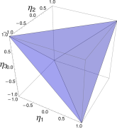
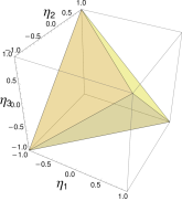
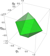
Figure 2: Geometry of positive maps: For positive trace preserving single-qubit maps, the allowed signed singular values lie within a cube $\mathcal{C}$ defined in (14). Quantum channels corresponding to CPTP maps lie within the blue tetrahedron $\mathcal{T}_{\text{CP}}$ defined in (7), steering maps corresponding to CcPTP maps lie within the yellow tetrahedron $\mathcal{T}_{\text{CcP}}$ defined in (12). The maps with SSV inside the intersection of $\mathcal{T}_{\text{CP}}$ and $\mathcal{T}_{\text{CcP}}$ (green octahedron) are called superpositive. These maps only produce classical correlations corresponding to separable states or entanglement breaking channels, but can also be generated by mixtures of quantum correlations.

III.4 Positive maps

We have seen that a quantum channel is a CPTP map and that a steering map is a CcPTP map. Both of them are necessarily positive maps. But are there positive maps that are neither CcP nor CP? Or are there maps that are even both? This issue is nicely worked out in (Bengtsson and Życzkowski, 2006, chapter 11). We shortly review this for unital qubit maps. Since we still deal with linear maps, it is straightforward that also every unital positive one-qubit map can be described by a $3\times 3$ correlation matrix. Hence we can also analyze its SSV. The allowed SSV are inside the cube $\mathcal{C}$ defined by (Bengtsson and Życzkowski, 2006, FIG.11.3)

$$\mathcal{C}\equiv\left\{\boldsymbol{x}|-1\leq x_{i}\leq 1\text{ for }i=1,2,3\right\}.$$ (14)

This is illustrated in FIG.2. Note again that we only treat unital maps.
We see that there are positive maps which are neither CP nor CcP. According to the Størmer-Woronowicz theorem (see e.g. (Bengtsson and Życzkowski, 2006, p. 258)) every positive qubit map is decomposable, i.e. it can be written as a convex combination of a CP and a CcP map. Maps that are both CP and CcP are called super positive (SP). The set of allowed SSV of the correlation matrices of these maps forms an octahedron (green region in FIG.2) given as

$$\mathcal{O}_{\text{SP}}=\text{Conv}\left(\{\pm\hat{e}_{i}|i\in{x,y,z}\}\right),$$ (15)

where $\hat{e}_{i}$ denotes the unit vector along the $i$-axis. These correlations are generated by entanglement breaking quantum channels Ruskai (2003) and steering maps based on separable states Jevtic et al. (2014). When such classical correlations are observed one cannot infer anything about the causal structure (Ried et al., 2015, p.10 of supplementary information).
For higher dimensional systems things change. Already for three dimensional maps, i.e. qutrit maps, there exist positive maps, that cannot be represented as a convex combination of a CP and a CcP map (Bengtsson and Życzkowski, 2006, chapter 11.1). In the next section we discuss how much information about causal influences we can obtain by looking only at the SSV related to the correlations Alice and Bob can observe in a bipartite experiment.

IV Causal explanation of unital positive maps

IV.1 Setting

We now tackle the problem of causal inference in the two-qubit scenario Ried et al. (2015). The setting is as follows. An experimenter, Alice, sits in her laboratory. She opens her door just long enough to obtain a qubit in a (locally) completely mixed state and closes the door again. She performs an projective measurement in any of the Pauli-states, records her outcome, opens her door again and puts the qubit in the now collapsed state outside. Apart from the qubit she has no way of interacting with the environment. Some time later another experimenter, Bob, opens the door of his laboratory and obtains a qubit. Also he measures in the eigenbasis of one of the Pauli matrices and records the outcome. They repeat this procedure a large (ideally: an infinite) number of times. Then they meet and analyze their joint measurement outcomes. These define the probabilities $P(a,b|j,i)$ for the outcomes $a\in\{-1,1\}$ and $b\in\{-1,1\}$ of Alice’s and Bob’s measurements, given they measured in the eigenbasis of the $j$th and $i$th Pauli matrix, respectively. For the marginals we assume $P(a|j,i)=\sum_{b}P(a,b|j,i)=1/2\,\,\forall a\in\{-1,1\}$ and accordingly for Bob. They are thus able to define a correlation matrix $M$ with elements

$$M_{ij}=2P(b=1|j,i,a=1)-1=\braket{\sigma_{j}\sigma_{i}},$$ (16)

where $P(b=1|j,i,a=1)$ is the probability that Bob obtains outcome $1$ when measuring the observable $\sigma_{i}$, conditioned on Alice’s measurement of $\sigma_{j}$ with outcome $1$, and $\braket{\sigma_{j}\sigma_{i}}$ denotes the expectation value of the product of Alice’s $\sigma_{j}$ and Bob’s $\sigma_{i}$ measurement outcomes.
The correlation matrix defines a unique positive trace preserving unital map $\mathcal{M}:\rho_{A}\mapsto\rho_{B}$. They are guaranteed one of the following three possibilities: either they measured the same qubit, which was propagated in terms of a unital quantum channel $\mathcal{E}$ from Alice to Bob; or that they each measured one of the two qubits in a unital bipartite state $\rho_{AB}$ acting as a common cause, and hence the correlations where caused by the corresponding steering map $\mathcal{S}$; or that the map from $\rho_{A}$ to $\rho_{B}$ is a probabilistic mixture where with probability $p$ the steering map $\mathcal{S}$ was realized and with probability $(1-p)$ the quantum channel $\mathcal{E}$, that is

$$\mathcal{M}=(1-p)\mathcal{E}+p\mathcal{S},$$ (17)

with the “causality parameter” $p\in[0,1]$.

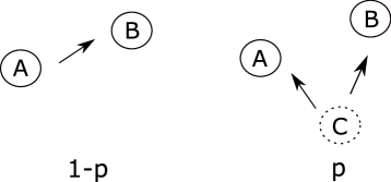
Figure 3: DAG: The DAGs of our setting. On the left side with probability $(1-p)$ a quantum channel $\mathcal{E}$ is realized, causing correlations between Alice ($A$) and Bob ($B$). On the right side, occuring with probability $p$, the correlations are caused by an unobserved source $C$ that outputs the state $\rho_{AB}$ generating correlations through the steering map $\mathcal{S}$.

The task of Alice and Bob is now to find the true value of $p$ and possibly also the nature of $\mathcal{S}$ and $\mathcal{E}$. In general there does not exist a unique solution and in this case they want to find the values of $p$ for which maps of the form (17) explain the observed correlations.
As we mentioned in the previous section, every positive one qubit map is decomposable, so a possible explanation always exists. The decomposition (17) can be given a causal interpretation, where $\mathcal{E}$ is considered to be a cause-effect explanation of the correlations and $\mathcal{S}$ a common-cause.
In the following subsections we give bounds on the causality parameter $p$ and then consider some extremal cases. In subsection IV.4 we generalize a part of the work of Ried et al. Ried et al. (2015) and see how additional assumptions on the nature of $\mathcal{E}$ and $\mathcal{S}$ can lead to a unique solution.

IV.2 Possible causal explanations

Definition IV.1

$p$-causality/$p$-decomposability: A single qubit unital positive trace preserving map $\mathcal{M}$ is called $p$-causal/$p$-decomposable with $p\in[0,1]$, if it can be written as

$$\mathcal{M}=(1-p)\mathcal{E}+p\mathcal{S},$$ (18)

with $\mathcal{E}$ ($\mathcal{S}$) being a CPTP (CcPTP) unital qubit map. Eq.(18) is called a $p$-decomposition of $\mathcal{M}$.

In the following let $M,E,S$ denote the correlation matrices of $\mathcal{M},\mathcal{E},\mathcal{S}$, and $\boldsymbol{\eta}^{\mathcal{M}},\boldsymbol{\eta}^{\mathcal{E}},\boldsymbol{\eta}^{\mathcal{S}}$ the SSV of $M,E,S$, respectively. We first investigate for a fixed $p$ what the possible SSV of the correlation matrix of a map $\mathcal{M}$ are, such that $\mathcal{M}$ is $p$-causal. This leads to the following theorem:

Theorem IV.1

Signed singular values of $p$-causal maps
Let $\mathcal{M}$ be a positive unital trace preserving qubit map with associated SSV given by $\boldsymbol{\eta}^{\mathcal{M}}$. Let $p\in[0,1]$ be fixed. Then the following statement holds:

$$\mathcal{M}\text{ is $p$-causal}\Leftrightarrow\boldsymbol{\eta}^{\mathcal{M}}\in\mathcal{C}_{p},$$ (19)

where

$$\mathcal{C}_{p}=\text{Conv}\left(\left\{(1-p)\boldsymbol{v}_{i}^{\text{CP}}+p\boldsymbol{v}_{j}^{\text{CcP}}|i,j\in\{1,2,3,4\}\right\}\right),$$ (20)

where the vertices $\boldsymbol{v}_{i}^{\text{CP}}$ of CP maps are given in (8), and the vertices $\boldsymbol{v}_{j}^{\text{CcP}}$ of CcP maps in (13).

Proof. "$\Leftarrow$": From (20) we see that

$$\boldsymbol{\eta}^{\mathcal{M}}\in\mathcal{C}_{p}\Leftrightarrow\exists\left(p_{ij}\geq 0,\;\sum_{i,j=1}^{4}p_{ij}=1\right):\boldsymbol{\eta}^{\mathcal{M}}=\sum_{i,j=1}^{4}p_{ij}\left((1-p)\boldsymbol{v}_{i}^{\text{CP}}+p\boldsymbol{v}_{j}^{\text{CcP}}\right).$$

Now define $q_{i}\equiv\sum_{j}p_{ij}$ and $r_{j}\equiv\sum_{i}p_{ij}$. Clearly $q_{i},r_{j}\geq 0$ and $\sum_{i}q_{i}=\sum_{j}r_{j}=1$. We can then write

$$\boldsymbol{\eta}^{\mathcal{M}}=(1-p)\sum_{i}q_{i}\boldsymbol{v}_{i}^{\text{CP}}+p\sum_{j}r_{j}\boldsymbol{v}_{j}^{\text{CcP}}=(1-p)\,\boldsymbol{\eta}^{\mathcal{E}}+p\,\boldsymbol{\eta}^{\mathcal{S}},$$

with $\boldsymbol{\eta}^{\mathcal{E}}\equiv\sum_{i}q_{i}\boldsymbol{v}_{i}^{\text{CP}}\in\mathcal{T}_{\text{CP}}$ and $\boldsymbol{\eta}^{\mathcal{S}}\equiv\sum_{j}r_{j}\boldsymbol{v}_{j}^{\text{CcP}}\in\mathcal{T}_{\text{CcP}}$. We herewith explicitly constructed a $p$-decomposition of $\mathcal{M}$ where the correlation matrices of $\mathcal{E}$ and $\mathcal{S}$ have their SSV-decomposition involving the same rotations as the SSV-decomposition of the correlation matrix of $\mathcal{M}$.

"$\Rightarrow$": Let $p$ be fixed. Suppose that $\mathcal{E}$ and $\mathcal{S}$ are both extremal maps, i.e. $\boldsymbol{\eta}^{\mathcal{E}}$ and $\boldsymbol{\eta}^{\mathcal{S}}$ are given by one of the vertices defined in (8) and (13), respectively, and without loss of generality we assume that these are $\boldsymbol{v}_{1}^{\text{CP}}$ and $\boldsymbol{v}_{1}^{\text{CcP}}$ (this is justified as taking another vertex leads to the same result). Define $A=(1-p)E$ and $B=pS$, where $A$ has SSV $(1-p,1-p,1-p)$ and B has SSV $(-p,-p,-p)$. In the Appendix we prove theorem VI.1 that restricts the possible SSV of $A+B$. For our case it gives

$$SSV(M)\in\mathcal{C}_{p}.$$

Now suppose $\mathcal{E}$ and $\mathcal{S}$ are not extremal maps. Since the SSV of those are simply convex combinations of the SSV of the extremal maps, it follows that also for such maps the signed singular values of $M$ lie within $\mathcal{C}_{p}$.   

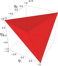
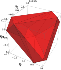
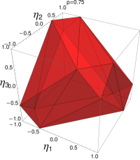
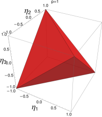
Figure 4: Signed singular values of $p$-causal maps: Set of attainable vectors of signed singular values associated with $\mathcal{M}$ in (17) for different values of $p$. By theorem IV.1, for fixed $p$ there exists a CPTP map $\mathcal{E}$ and a CcPTP map $\mathcal{S}$ such that $\mathcal{M}$ is given by (17) if and only if the vector of signed singular values $\boldsymbol{\eta}^{\mathcal{M}}$ of the correlation matrix of $\mathcal{M}$ is in $\mathcal{C}_{p}$ defined in (20).

We have seen that for a given value of $p$ the allowed SSV associated with a positive map $\mathcal{M}$ that is $p$-causal lie within $\mathcal{C}_{p}$ given in (20). We now turn the task around and go back to the causal inference scenario. Given a positive map $\mathcal{M}$ we want to tell if we can bound the causality parameter $p$. We will do this based on the following definition:

Definition IV.2

Causal interval $I_{\mathcal{M}}$:
For a given positive unital qubit map $\mathcal{M}$ we define the interval of possible causal explanations (for short: the causal interval) $I_{\mathcal{M}}$, such that $\mathcal{M}$ is $p$-causal if and only if $p\in I_{\mathcal{M}}$.

Since every qubit map is decomposable (Bengtsson and Życzkowski, 2006, p.258) the causal interval is always non empty, $I_{\mathcal{M}}\neq\emptyset$.

Theorem IV.2

Let $\mathcal{M}$ be a positive unital qubit map, with associated signed singular values $\boldsymbol{\eta}^{\mathcal{M}}$ (we assume $\eta^{\mathcal{M}}_{i}\geq 0$ for $i=1,2$). Then the causal interval of $\mathcal{M}$ is given by

$$p_{\text{max}} =\min\left(\frac{3-\boldsymbol{\eta}^{\mathcal{M}}\cdot\boldsymbol{v}_{1}^{\text{CP}}}{2},1\right),$$ (21)

$$p_{\text{min}} =\max\left(\frac{\boldsymbol{\eta}^{\mathcal{M}}\cdot\boldsymbol{v}_{4}^{\text{CcP}}-1}{2},0\right),$$ (22)

with $\boldsymbol{v}_{1}^{\text{CP}}=(1,1,1)^{T}$ ($\boldsymbol{v}_{4}^{\text{CcP}}=(1,1,-1)^{T}$) defining a vertex of the CPTP (CcPTP) tetrahedron $\mathcal{T}_{CP}$ ($\mathcal{T}_{CcP}$).

Note that the assumption $\eta^{\mathcal{M}}_{i}\geq 0$ for $i=1,2$ can always be met, using the unitary freedom in the decomposition in the right way.
Proof. We show the theorem for $p_{\text{max}}$, the determination of $p_{\text{min}}$ can be treated in an analogue way.
First we check if $\mathcal{M}$ is a CcPTP map, by checking if $\boldsymbol{\eta}^{\mathcal{M}}\in\mathcal{T}_{\text{CcP}}$. If it is CcPTP then $p_{\text{max}}=1$, trivially.

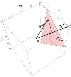
Figure 5: Sketch for proof of theorem IV.2: The value of $p_{\text{max}}$ is determined through the projection of $\boldsymbol{\eta}^{\mathcal{M}}$ onto $\boldsymbol{v}_{1}^{\text{CP}}$, which is given by $\boldsymbol{u}$. The red triangle is one of the facets of $\mathcal{C}_{p_{\text{max}}}$.

Now suppose it is not CcPTP. $p_{\text{max}}$ is then given such that $\boldsymbol{\eta}^{\mathcal{M}}\in\mathcal{C}_{p_{\text{max}}}$ but $\boldsymbol{\eta}^{\mathcal{M}}\notin\mathcal{C}_{p^{\prime}}$ with $p^{\prime}\in(p_{\text{max}},1]$. This implies that $\boldsymbol{\eta}^{\mathcal{M}}$ lies on the surface of $\mathcal{C}_{p_{\text{max}}}$. Since we assumed $\eta^{\mathcal{M}}_{i}\geq 0$ for $i=1,2$, the critical facet of $\mathcal{C}_{p_{\text{max}}}$ is the one which is perpendicular to $\boldsymbol{v}^{\text{CP}}_{1}$ and has the vertices $(1,1,1-2p_{\text{max}})^{T},(1,1-2p_{\text{max}},1)^{T},(1-2p_{\text{max}},1,1)^{T}$ (see FIG.5). Since this facet is perpendicular to $\boldsymbol{v}^{\text{CP}}_{1}$, $\boldsymbol{\eta}^{\mathcal{M}}$ lies on this facet if its projection onto $\boldsymbol{v}_{1}^{\text{CP}}$ equals the vector pointing from the origin to the intersection of the facet and $\boldsymbol{v}^{\text{CP}}_{1}$, given as $\boldsymbol{u}\equiv(1-(2/3)\,p_{\text{max}})\boldsymbol{v}^{\text{CP}}_{1}$, see Fig.5. Hence we get the following equation

$$\frac{1}{3}\boldsymbol{v}^{\text{CP}}_{1}(\boldsymbol{v}^{\text{CP}}_{1}\cdot\boldsymbol{\eta}^{\mathcal{M}})\overset{!}{=}\boldsymbol{u}$$ (23)

$$\Leftrightarrow\boldsymbol{v}^{\text{CP}}_{1}\cdot\boldsymbol{\eta}^{\mathcal{M}}=3-2p_{\text{max}}$$ (24)

$$\Leftrightarrow p_{\text{max}}=\frac{3-\boldsymbol{\eta}^{\mathcal{M}}\cdot\boldsymbol{v}^{\text{CP}}_{1}}{2}.$$ (25)

 

IV.3 Extremal cases

In the previous section we found the general form of the causal interval $I_{\mathcal{M}}$ for an observed map $\mathcal{M}$. We now analyze the extremal cases where the interval reduces to a single value or on the other hand the interval is given as $I_{\mathcal{M}}=[0,1]$.
As already noted in (Ried et al., 2015, Table 1.) there are extremal cases that allow for a complete solution of the problem even without any additional constraints. This is the case if $\boldsymbol{\eta}^{\mathcal{M}}$ equals one of the vertices of the cube of positive maps, see Fig. 2. The solution is then either $p=0$ (pure cause-effect) if the SSV are all positive or exactly two are negative or $p=1$ (pure common-cause) if the SSV are all negative or exactly one positive. The exact reconstruction of $\mathcal{E}$ or $\mathcal{S}$ in this cases is trivial.
Interestingly, with theorem IV.2 we can show that every point on the edges of the cube $\mathcal{C}$ defined in (14) gives us a unique solution without additional constraints:
Proof. Let $\mathcal{M}$ be a positive map and $M$ be the corresponding correlation matrix with $M=R_{1}\eta^{\mathcal{M}}R_{2}$ where $\eta^{\mathcal{M}}=\text{diag}(\boldsymbol{\eta}^{\mathcal{M}})$ with the signed singular values $\boldsymbol{\eta}^{\mathcal{M}}=(1,1,1-2p)^{T},\;p\in[0,1]$, and two rotations $R_{1},R_{2}\in SO(3)$. Due to the freedom in $R_{1}$ and $R_{2}$ this describes all maps with corresponding vector of SSV on one of the edges of the cube $\mathcal{C}$ defined in (14). According to theorem IV.2 we find

$$p_{\text{max}} =\min\left(\frac{3-\boldsymbol{\eta}^{\mathcal{M}}\cdot\boldsymbol{v}_{1}}{2},1\right)=\frac{3-\left(2+(1-2p)\right)}{2}=p,$$ (26)

$$p_{\text{min}} =\max\left(\frac{\boldsymbol{\eta}^{\mathcal{M}}\cdot\boldsymbol{v}_{4}^{\text{CcP}}-1}{2},0\right)=\frac{2-(1-2p)-1}{2}=p.$$ (27)

By theorem VI.1 it follows, that the maps $\mathcal{E}$ and $\mathcal{S}$ in the decomposition (17) necessarily correspond to extremal points in $\mathcal{T}_{\text{CP}}$ and $\mathcal{T}_{\text{CcP}}$ defined in (7) and (12) (unitary channel and maximally entangled state). It is then obvious that

$$M=R_{1}\left((1-p)\text{diag}(\boldsymbol{v}^{\text{CP}}_{1})+p\,\text{diag}(\boldsymbol{v}^{\text{CcP}}_{4})\right)R_{2}$$ (28)

is the only possible solution.   

In the other extreme case, if the map $\mathcal{M}$ is superpositive, i.e. CP and CcP (see Figure 2), it could be explained by a pure CPTP, a pure CcPTP map, or any convex combination of those two. Therefore one cannot give any restrictions of possible values of $p$ (Ried et al., 2015, III.E of supplementary information).
Proof. Let $\mathcal{M}$ be a superpositive map. There exists a SSV decomposition of its correlation matrix for which $\boldsymbol{\eta}^{\mathcal{M}}\in\mathcal{O}_{\text{SP}}$, defined in (15), and for which $\eta^{\mathcal{M}}_{i}\geq 0$ for $i=1,2$. Hence we can write $\boldsymbol{\eta}^{\mathcal{M}}=p_{1}\hat{e}_{x}+p_{2}\hat{e}_{y}+p_{3}\hat{e}_{z}+p_{4}(-\hat{e}_{z})$, with $\sum_{i}p_{i}=1$. The scalar product of each component of $\boldsymbol{\eta}^{\mathcal{M}}$ with $\boldsymbol{v}^{\text{CP}}_{1}=(1,1,1)^{T}$ is upper bounded by 1. Hence we have $\boldsymbol{\eta}^{\mathcal{M}}\cdot\boldsymbol{v}^{\text{CP}}_{1}\leq 1$ and with that eq. (21) evaluates to $p_{\text{max}}=1$. Analogously one finds $p_{\text{min}}=0$.   

IV.4 Additional assumptions / Causal inference with constrained classical correlations

So far we only assumed that our data is generated by a unital channel and a unital state (a state whose local partitions are completely mixed). We have seen that in some extreme cases a unique solution to the problem can be found. Ried et al. showed that one can always find a unique solution for $p$ if one restricts the channel to unitary channels and the bipartite states to maximally entangled pure states Ried et al. (2015). Furthermore, it is then possible to reconstruct the channel and the state up to binary ambiguity, meaning there are two explanations leading to the same observed correlations. The ellipsoids associated with unitary channels and maximally entangled states are spheres with unit radius and the SSV of their correlation matrices correspond to the vertices of $\mathcal{T}_{\text{CP}}$ and $\mathcal{T}_{\text{CcP}}$ respectively .
In the following we investigate this scenario again, but add a known amount of noise in the channel or in the bipartite state. For the channel this is done by mixing the unitary evolution with a completely depolarizing channel Nielsen and Chuang (2010). The completely depolarizing channel maps every Bloch-vector to the origin, $\rho\mapsto\frac{\mathbb{1}}{2}$ and hence is represented by the zero matrix. The ellipsoid associated with the mixture of a completely depolarizing channel with a unitary channel thus results in a shrinked sphere. For strong enough noise the result eventually becomes an entanglement breaking channel, which only produces “classical” correlations Ruskai (2003). Due to the unitary freedom compared to standard depolarizing channels, we call these channels generalized depolarizing channel. For the state we mix a pure maximally entangled state with the completely mixed state, whose correlation matrix is given by the zero-matrix. We call the state a generalized Werner state, in the sense that instead of a convex combination of a singlet and a completely mixed state Werner (1989) we allow the convex combination of an arbitrary maximally entangled state with the completely mixed state. States at a certain threshold of noise become separable and the correlations become “classical” Jevtic et al. (2014). We will then see that even when confronted with purely classical correlations, if we have enough a-priori-knowledge about the data generation, i.e. we know the amount of noise, we can still find a solution analogous to Ried et al. (2015), in the sense of determining uniquely the parameter $p$, and the channel and the state up to binary ambiguity. We will first keep the unitary channel and start with a generalized Werner-state and show how one can recreate the scenario of Ried et al. Then we will add the noise in the channel.

IV.4.1 Solution of the causal inference problem using generalized Werner states

The analysis follows closely in spirit section III.D in the supplementary information in Ried et al. (2015). We start again with equation (17) and assume that the steering map $\mathcal{S}$ is generated by a shared generalized Werner state $\rho_{AB}=\epsilon\frac{\mathbb{1}}{4}+(1-\epsilon)|\psi\rangle\langle\psi|$, where the parameter $\epsilon\in[0,1)$ is known and fixed in advance and $|\psi\rangle$ is an unknown maximally entangled pure state. The map $\mathcal{E}$ is generated by an unknown unitary channel $U$.
Since $\epsilon$ is fixed, the class of allowed explanations is completely defined up to unitary freedom in the channel and in the state. Hence the number of free parameters is the same as in the case considered in Ried et al. (2015), which coincides with the case $\epsilon=0$. For $\epsilon>2/3$ the state $\rho_{AB}$ becomes separable, i.e. is not entangled anymore, see Werner (1989) and Fig.5 in the supplementary information of Jevtic et al. (2014). But the reconstruction works independently of $\epsilon$. Hence, we see here that the possibility of reconstruction hinges not on the entanglement in $\rho_{AB}$ but on the prior knowledge we have about $\rho_{AB}$.

The correlation matrix corresponding to the generalized Werner-state is simply the one of a maximally entangled state shrinked by a factor $1-\epsilon$ and will thus be denoted $(1-\epsilon)S$, where $S$ is the correlation matrix corresponding to a maximally entangled state. Thus in our scenario the information Alice and Bob obtain characterizes the matrix

$$M=p(1-\epsilon)S+(1-p)E.$$ (29)

The ellipsoid is described by the eigenvalues and -vectors of $MM^{T}$. The eigenvectors correspond to the direction of the semi axes and the squareroots of the eigenvalues are their lengths. There is one degenerate pair and another single one. The eigenvector corresponding to the non-degenerate semi axis is parallel to $\boldsymbol{n}$ which is defined as the axis on which the images of $S$ and $E$ are diametrically opposed. Hence the length of this semi axis is $l_{1}=|1-p-p(1-\epsilon)|$. Furthermore we have

$$\text{sign}(\det M)=\text{sign}(1-p-p(1-\epsilon)),$$

if $l_{1}>0$ and $\det M=0$ if $l_{1}=0$. Thus if we calculate the length of this semi axis we can already determine the causality parameter $p$ as

$$l_{1}=|1-2p+p\epsilon|\Leftrightarrow p=\frac{1\mp l_{1}}{2-\epsilon},$$ (30)

where the ambiguity is solved by considering the sign of $\det M$.
Now that we have $p$ and $\epsilon$ at hand we can define a new map with correlation matrix

$$M^{\prime}\equiv\frac{1}{1-p\epsilon}M=\frac{p(1-\epsilon)}{1-p\epsilon}S+\frac{1-p}{1-p\epsilon}E\equiv p^{\prime}S+(1-p^{\prime})E,$$ (31)

where we defined

$$p^{\prime}\equiv\frac{p(1-\epsilon)}{1-p\epsilon},$$ (32)

$$1-p^{\prime}=1-\frac{p(1-\epsilon)}{1-p\epsilon}=\frac{1-p\epsilon-p(1-\epsilon}{1-p\epsilon}=\frac{1-p}{1-p\epsilon}.$$ (33)

The properties of the ellipsoid can also be found in the SSV decomposition of the correlation matrix

$$M=R_{1}DR_{2},\qquad\text{with }D=\text{diag}(\boldsymbol{\eta}^{\mathcal{M}})\text{ and }\;R_{1},R_{2}\in SO(3).$$ (34)

The absolute values of the entries of $\boldsymbol{\eta}^{\mathcal{M}}$ equal the lengths of the semi axes of the ellipsoid and we choose $R_{1}$ and $R_{2}$ such that $\eta^{\mathcal{M}}_{1}=\eta^{\mathcal{M}}_{2}$. The axis on which the images of $S$ and $E$ are diametrically opposed is then given by the last column of $R_{1}$, i.e. $\hat{n}=R_{1}\hat{e}_{3}$. The length of this axis is $l_{1}=|\eta^{\mathcal{M}}_{3}|$.
In (31) the promise is given that $S$ is the correlation matrix of a maximally entangled state and that $E$ is the correlation matrix of a unitary channel. The reconstruction of those is extensively studied in the supplementary information of Ried et al. (2015). With the method presented there we find the value of $p^{\prime}$ and can restore the correlation matrices corresponding to $U$ and $|\psi\rangle$ up to a binary ambiguity, and hence solve the causal inference problem. We review this in terms of SSV and discuss where the binary ambiguity arises.
Starting from the l.h.s. of (31) the goal is to determine $p^{\prime},S,$ and $M$ on the r.h.s. Consider the SSV decomposition of the correlation matrix

$$M^{\prime}=R^{\prime}_{1}D^{\prime}R^{\prime}_{2},\qquad\text{with }D^{\prime}=\text{diag}(\boldsymbol{\eta}^{\mathcal{M^{\prime}}})\text{ and }R_{1}^{\prime},R_{2}^{\prime}\in SO(3).$$ (35)

The absolute values of the entries of $\boldsymbol{\eta}^{\mathcal{M^{\prime}}}$ equal the lengths of the semi axes of the ellipsoid and we choose $R^{\prime}_{1},R^{\prime}_{2}$ s.t. $\eta_{1}^{\mathcal{M^{\prime}}}=\eta_{2}^{\mathcal{M^{\prime}}}$. The axis on which the images of $S$ and $E$ are diametrically opposed is then given by the last column of $R^{\prime}_{1}$, i.e. $\hat{n}^{\prime}=R^{\prime}_{1}\hat{e}_{3}$. The length of this axis is $l^{\prime}_{1}=|\eta_{3}^{\mathcal{M^{\prime}}}|$. However, the direction of $\hat{n}^{\prime}$, depending on the choice of $R^{\prime}_{1}$ and $R^{\prime}_{2}$, cannot be determined uniquely and allows two possible solutions $\pm\hat{n}^{\prime}$. The parameter $p^{\prime}$ is determined by the length $l_{1}^{\prime}$ and can be calculated as

$$p^{\prime}=\frac{1-\left(\text{sign}\det(M^{\prime})\right)l_{1}^{\prime}}{2},$$ (36)

and if $\det(M^{\prime})=0$ we have $p^{\prime}=1/2$. If $p^{\prime}=0$ or $p^{\prime}=1$ the reconstruction is trivial (of course in these cases one cannot reconstruct $S$ or $E$, respectively). If $p^{\prime}\in(0,1)$, we can define Ried et al. (2015)

$$r^{\prime} =|\eta_{1}^{\mathcal{M^{\prime}}}|,$$ (37)

$$\gamma^{\prime} =2\arcsin\left(\sqrt{\frac{1-r^{\prime 2}}{4(p^{\prime}-{p^{\prime}}^{2})}}\right),$$ (38)

$$\gamma_{2}^{\prime} =\arccos\left(\frac{1+r^{\prime 2}-\left[2p^{\prime}\sin\frac{\gamma^{\prime}}{2}\right]}{2r^{\prime}}\right).$$ (39)

The reconstruction of the correlation matrices $S$ and $E$ can then be done, c.f. eq. (58) and (59) in the supplementary information of Ried et al. (2015):

$$E =R_{\hat{n}^{\prime},\gamma^{\prime}_{2}}S_{\perp\hat{n}^{\prime},1/r^{\prime}}S_{\hat{n}^{\prime},1/(1-2p^{\prime})}M^{\prime},$$ (40)

$$S =R_{\hat{n}^{\prime},-\gamma^{\prime}+\gamma^{\prime}_{2}}S_{\perp\hat{n}^{\prime},1/r^{\prime}}S_{\hat{n}^{\prime},1/(2p^{\prime}-1)}M^{\prime},$$ (41)

where $R_{\hat{n},\alpha}$ indicates a rotation about axis $\hat{n}$ with rotation angle $\alpha$, $S_{\hat{n}^{\prime},1/(1-2p^{\prime})}$ a scaling along $\hat{n}^{\prime}$ by a factor $1/(1-2p^{\prime})$ and $S_{\perp\hat{n}^{\prime},1/r^{\prime}}$ a scaling of the plane perpendicular to $\hat{n}^{\prime}$ by a factor $1/r^{\prime}$. From (40) and (41) we see that a reconstruction of $E$ and $S$ is not possible if $p^{\prime}=1/2$.
Let us summarize what we can infer about the causation of $M$ given in (29):

• The causality parameter $p$ can be determined uniquely in all cases, see eq.(30).

• If $r^{\prime}=0$ or $p^{\prime}=1/2$ then $S$ and $E$ cannot be determined,

• else we can determine two sets of solutions for $E$ and $S$ given by (40) and (41), distinguished by the choice of direction of $\hat{n}^{\prime}$.

On the other hand, if we do not have prior knowledge of $\epsilon$, then in general we cannot determine $p$ with (30). This ambiguity can easily be illustrated by looking at an example:
Take $U=\sigma_{x}$ and $|\psi\rangle=\frac{|00\rangle-|11\rangle}{\sqrt{2}}$. We then have:

$$E=\text{diag}(1,-1,-1),\qquad S=\text{diag}(-1,1,1).$$

Combining this for arbitrary $\epsilon$ and $p$ gives

$$M=\text{diag}(1-p\epsilon,-(1-p\epsilon),-(1-p\epsilon)).$$

Hence for all values of the parameters where $p\epsilon=\text{cons.}$, the measurement statistics for Alice and Bob are exactly the same and there is no way to distinguish different pairs of values.

Analogously to using a generalized Werner state for the steering map, we can also use a generalized depolarizing channel. Then, with prior knowledge of the amount of noise, we can still find a complete solution even though the resulting channel might be entanglement breaking.

IV.4.2 Generalized depolarizing channel and generalized Werner state

We shall now consider the case where both the channel as well as the state are mixed with a known amount of noise. Therefore we take $S^{\prime}=(1-\epsilon_{c})S$ for a generalized Werner state (thus $S$ corresponds again to a rotated and inverted Bloch-sphere) and $E^{\prime}=(1-\epsilon_{e})E$ for a generalized depolarizing channel. We again assume $\epsilon_{e}\,\in(0,1)$ and $\epsilon_{c}\,\in(0,1)$ to be known. We then have

$$M=(1-p)(1-\epsilon_{e})E+p(1-\epsilon_{c})S.$$ (42)

The reconstruction works as follows. Without loss of generality we assume $\epsilon_{e}\leq\epsilon_{c}$ (in the other case we just have to make the reconstruction discussed in the previous subsection for the entanglement breaking channel and not for the Werner-state). The only thing we have to do is to divide by $(1-\epsilon_{e})$ to restore the problem of the previous section

$$M^{\prime}=\frac{M}{1-\epsilon_{e}}=(1-p)E+p\frac{1-\epsilon_{c}}{1-\epsilon_{e}}S\equiv(1-p)E+p(1-\epsilon)S,$$

with $1-\epsilon\equiv\frac{1-\epsilon_{c}}{1-\epsilon_{e}}$. The rest can then be solved as in the previous subsection.
Again we remark that nothing changes if we have $\epsilon_{c}>2/3$ and $\epsilon_{e}>2/3$ even though at that transition the states become separable and the channels entanglement-breaking, respectively.

V Discussion

In this work we extended the results initially found by Ried et al. Ried et al. (2015). We introduced an active and a passive quantum-observational scheme as analogies to the classical observational scheme. The passive quantum-observational scheme does not allow for an advantage over classical casual inference. In the active quantum observational scheme Alice and Bob can freely choose their measurement bases, which in principle allows for signaling. However, we investigated the quantum advantage over classical causal inference in a scenario where signaling is not possible in the active quantum observation scheme, as Alice’ incoming state is completely mixed.

We showed how the geometry of the set of signed singular values (SSV) of correlation matrices representing positive maps of the density operator $\rho_{A}\mapsto\rho_{B}$ determines the possibility to reconstruct the causal structure linking $\rho_{A}$ and $\rho_{B}$. We showed that there are more cases than previously known for which a complete solution of the causal inference problem can be found without additional constraints, namely all correlations created by maps whose signed singular values of the correlation matrix lie on the edges of the cube of positive maps $\mathcal{C}$ defined in (14). A necessary and sufficient condition for this is that the state is maximally entangled, that the channel is unitary, and that the corresponding correlation matrices have a SSV decomposition involving the same rotations.
For correlations guaranteed to be produced by a mixture of a unital channel and a unital bipartite state, we quantified the quantum advantage by giving the intervals for possible values of the causality parameter $p$. Here, in order to constrain $p$, and hence have an advantage over classical causal inference, it is necessary that the correlations were caused by an entangled state and/or an entanglement preserving channel. This is because correlations caused by any mixture of a separable state and an entanglement breaking quantum channel always describe super-positive maps. According to theorem IV.2 the causal interval for any super-positive map $\mathcal{M}$ is $I_{\mathcal{M}}=[0,1]$. Hence, super-positive maps do not allow any causal inference.
Things change when we further strengthen the assumptions on the data generating processes and allow only unitary freedom in the state, corresponding to a generalized Werner state with given degree of noise $\epsilon_{c}$, or unitary freedom in the channel, corresponding to a generalized depolarizing channel with given degree of noise $\epsilon_{e}$. We showed that in this scenario the causality parameter $p$ can always be uniquely determined and in most cases the state and the channel can be reconstructed up to binary ambiguity. For $\epsilon_{c}>2/3$ the state becomes separable and for $\epsilon_{e}>2/3$ the channel entanglement breaking but still causal inference is feasible. Therefore entanglement and entanglement preservation are not a necessary condition in this scenario. The assumptions on the data generating processes, i.e. a-priori knowledge of $\epsilon_{c}$ and $\epsilon_{e}$, are strong enough, such that even correlations corresponding to super-positive maps reveal the underlying causal structure.

VI Appendix

Signed singular values of sums of matrices

Let $A$ be a $n\times n$ real matrix. A possible singular value decomposition (SVD) of $A$ is given as

$$A=O_{1}DO_{2},$$ (43)

where $O_{1,2}$ are orthogonal matrices ($O_{i}O_{i}^{T}=\mathbb{1}$) and $D$ is a positive semi-definite diagonal matrix $D=\text{diag}(\sigma_{1}^{A},...,\sigma_{n}^{A})$, with $\sigma_{i}^{A}$ called the (absolute) singular values (SV) of $A$. The matrices in (43) are not uniquely defined and all possible permutations of the singular values on the diagonal of $D$ are possible for different orthogonal matrices $O_{1}$ and $O_{2}$. We use this freedom to write the SV in canonical order, $\sigma_{1}^{A}\geq\sigma_{2}^{A}\geq...\geq\sigma_{n}^{A}$.
Example: We give two different SVDs of a $3\times 3$ matrix $B$

$$B\equiv\begin{pmatrix}-1&0&0\\ 0&0&-3\\ 0&2&0\end{pmatrix} =\begin{pmatrix}1&0&0\\ 0&0&-1\\ 0&1&0\end{pmatrix}\begin{pmatrix}1&0&0\\ 0&2&0\\ 0&0&3\end{pmatrix}\begin{pmatrix}-1&0&0\\ 0&1&0\\ 0&0&1\end{pmatrix}$$

$$=\begin{pmatrix}0&-1&0\\ 0&0&1\\ -1&0&0\end{pmatrix}\begin{pmatrix}3&0&0\\ 0&2&0\\ 0&0&1\end{pmatrix}\begin{pmatrix}0&0&1\\ 0&1&0\\ 1&0&0\end{pmatrix}.$$

The last decomposition gives the singular values of $B$ in canonical order $\sigma_{1}^{B}=3,\sigma_{2}^{B}=2$ and $\sigma_{3}^{B}=1$.
Next we call

$$A=R_{1}D^{\prime}R_{2}$$ (44)

the signed singular value decomposition (also called real singular values Amir-Moez and Horn (1958)) of $A$, where $R_{i}\in SO(n)$ are orthogonal matrices with determinant equal to one. In the $3\times 3$ scenario these correspond to proper rotations in $\mathbb{R}^{3}$. The diagonal matrix $D^{\prime}$ contains the signed singular values (SSV) of A. The SSV have the same absolute values as the SV but additionally can have negative signs. Concretely, the freedom in choosing $R_{1}$ and $R_{2}$ allows one to get any permutations of the SV on the diagonal of $D^{\prime}$ together with an even or odd number of minus signs, depending on whether $A$ has positive or negative determinant, respectively. If at least one singular value equals 0, the number of signs becomes completely arbitrary. Using the same matrix $B$ as above we give two different signed singular value decompositions as an example:

$$B\equiv\begin{pmatrix}-1&0&0\\ 0&0&-3\\ 0&2&0\end{pmatrix} =\begin{pmatrix}1&0&0\\ 0&0&-1\\ 0&1&0\end{pmatrix}\begin{pmatrix}-1&0&0\\ 0&2&0\\ 0&0&3\end{pmatrix}\begin{pmatrix}1&0&0\\ 0&1&0\\ 0&0&1\end{pmatrix}$$ (45)

$$=\begin{pmatrix}0&-1&0\\ 0&0&1\\ -1&0&0\end{pmatrix}\begin{pmatrix}3&0&0\\ 0&2&0\\ 0&0&-1\end{pmatrix}\begin{pmatrix}0&0&1\\ 0&1&0\\ -1&0&0\end{pmatrix}.$$ (46)

For the SSV decomposition we define a canonical order with the absolute values of the singular values sorted in decreasing order and only a negative sign on the last entry if the matrix has negative determinant, as in (46). The rotational freedom in (44) allows for arbitrary permutations of the order of singular values and addition of any even number of minus signs.
Confusion may arise since for example an $\mathbb{R}^{3}$ permutation matrix corresponding to a permutation of exactly two coordinates has determinant -1, so why would it be allowed? The point is, that we not only want to permute elements of a vector, but the diagonal elements of a matrix. We illustrate that by permuting two components of i) a vector and ii) a diagonal matrix.

$$P_{yz}\equiv\begin{pmatrix}1&0&0\\ 0&0&1\\ 0&1&0\end{pmatrix},\qquad\det P_{yz}=-1,$$ (47)

$$\textit{i) }P_{yz}\cdot\begin{pmatrix}a\\ b\\ c\end{pmatrix}=\begin{pmatrix}a\\ c\\ b\end{pmatrix},$$ (48)

$$\textit{ii) }P_{yz}\cdot\text{diag}(a,b,c)\cdot P_{yz}=\text{diag}(a,c,b)=(-P_{yz})\,\text{diag}(a,b,c)\,(-P_{yz}).$$ (49)

I.e. as $-P_{yz}=R_{\hat{\boldsymbol{x}}}(\pi/2)\cdot R_{\hat{\boldsymbol{y}}}(\pi)$ the effect of permuting the second and third diagonal entry of a diagonal matrix can also be obtained by proper rotations, and correspondingly for other permutations of the SSV. Hence all permutations of the SSV are allowed.

Fan Fan (1951) gave bounds on the SV of $A+B$ given the SV of two real matrices $A$ and $B$, derived from the corresponding results for eigenvalues of hermitian matrices and using that the matrix $\tilde{A}\equiv\begin{pmatrix}0_{n\times n}&A\\ A^{T}&0_{n\times n}\end{pmatrix}$ has the singular values of $A$ and their negatives as eigenvalues (Marshall and Olkin, 1979, p.243 for review). In the main part of this work we need a more constraining statement using the SSV, and thus taking the determinant of $A$, $B$, and $A+B$ into account as well. This leads to theorem VI.1. In the following we will denote with $\tilde{\boldsymbol{\sigma}}(A)$ the vector of canonical SSV of the $n\times n$ real matrix A. Since the product of two rotations is again a rotation it follows directly from (44) that

$$\tilde{\boldsymbol{\sigma}}(Q_{1}AQ_{2})=\tilde{\boldsymbol{\sigma}}(A),\;\forall Q_{1},Q_{2}\in SO(n).$$ (50)

Let $\boldsymbol{w}$ be a $n$-dimensional vector. We define

$$\Delta_{\boldsymbol{w}}\equiv\text{Conv}\left(\left\{\left.\left(s_{1}w_{\pi(1)},...,s_{n}w_{\pi(n)}\right)^{T}\right|s_{\nu}\in\{-1,1\}:\prod_{\nu}s_{\nu}=1,\pi\in S_{n}\right\}\right)$$ (51)

as the convex hull of all possible permutations $\pi\in S_{n}$ of the components of $\boldsymbol{w}$ multiplied with an even number of minus signs. Let now $\boldsymbol{w_{1}}$ and $\boldsymbol{w_{2}}$ be two $n$-dimensional vectors. We define

$$\Sigma_{\boldsymbol{w_{1}},\boldsymbol{w_{2}}}\equiv\left\{a+b|a\in\Delta_{\boldsymbol{w_{1}}},b\in\Delta_{\boldsymbol{w_{2}}}\right\}.$$ (52)

Figure 6 presents an illustration of the case $n=2$.

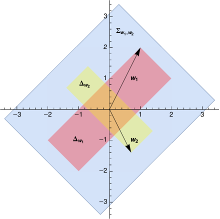
Figure 6: Illustration of theorem VI.1: Suppose we have two $2\times 2$ matrices $A$ and $B$ with SSV $\boldsymbol{w}_{1}$ and $\boldsymbol{w}_{2}$ respectively. The red and the yellow sets correspond to $\Sigma_{\boldsymbol{w}_{1}}$ and $\Sigma_{\boldsymbol{w}_{2}}$ defined by (51). By theorem VI.1 the vector of SSV of $A+B$ then lies within the blue set, defined by (52).

Theorem VI.1

Let $A$ and $B$ be two $n\times n$ real matrices whose SSV are known. Then

$$\tilde{\boldsymbol{\sigma}}(A+B)\in\Sigma_{\tilde{\boldsymbol{\sigma}}(A),\tilde{\boldsymbol{\sigma}}(B)}.$$ (53)

Proof. Let $A$ be a $n\times n$ real matrix and let $\boldsymbol{d}(A)$ denote the vector of diagonal entries of $A$. Thompson showed the following two statements about the diagonal elements of $A$ (Thompson, 1977, theorems 7 and 8)

$$i) \boldsymbol{d}(A)\in\Delta_{\tilde{\boldsymbol{\sigma}}(A)},$$ (54)

$$ii) \forall\boldsymbol{d}\in\Delta_{\tilde{\boldsymbol{\sigma}}(A)}\;\exists R_{1},R_{2}\in SO(n):\boldsymbol{d}=\boldsymbol{d}(R_{1}AR_{2}).$$ (55)

Now let $A$ and $B$ be two $n\times n$ real matrices. Let $R_{1},R_{2}\in SO(n)$ such that $\boldsymbol{d}(R_{1}(A+B)R_{2})=\tilde{\boldsymbol{\sigma}}(A+B)$. We then have

$$\tilde{\boldsymbol{\sigma}}(A+B)=\boldsymbol{d}(R_{1}(A+B)R_{2})=\boldsymbol{d}(R_{1}AR_{2})+\boldsymbol{d}(R_{1}BR_{2})\in\Sigma_{\tilde{\boldsymbol{\sigma}}(R_{1}AR_{2}),\tilde{\boldsymbol{\sigma}}(R_{1}BR_{2})}=\Sigma_{\tilde{\boldsymbol{\sigma}}(A),\tilde{\boldsymbol{\sigma}}(B)},$$

where the second equation follows from the linearity of matrix addition in every element and the last equality from (50).   
As mentioned above, results for the absolute singular values of $A+B$ have been known before. To complete, we show that the above proof works analogously for the corresponding statement on absolute singular values: Let $\boldsymbol{\sigma}(A)$ denote the vector of canonical absolute singular values of an $n\times n$ real matrix $A$, $\sigma_{1}(A)\geq\sigma_{2}(A)\geq...\geq\sigma_{n}(A)$. Let $B$ be another $n\times n$ real matrix. Then (Marshall and Olkin, 1979, chapter 9 G.1.d.)

$$\boldsymbol{\sigma}(A+B)\prec_{w}\boldsymbol{\sigma}(A)+\boldsymbol{\sigma}(B),$$ (56)

i.e. the vector of canonical singular values of $A+B$ is weakly majorized by the sum of the vectors of canonical singular values of $A$ and $B$. Weak majorization for two vectors $\boldsymbol{x}$ and $\boldsymbol{y}$ with $x_{1}\geq x_{2}\geq...\geq x_{n}$ and $y_{1}\geq y_{2}\geq...\geq y_{n}$ is defined as

$$\boldsymbol{x}\prec_{w}\boldsymbol{y}\Leftrightarrow\sum_{i=1}^{k}x_{i}\leq\sum_{i=1}^{k}y_{k}\;\forall k\in\left\{1,2,...,n\right\}.$$ (57)

To see (56) define $\Delta^{\prime}_{\boldsymbol{w}}$ analogously to (51) but without the constraint $\prod_{\nu}s_{\nu}=1$, i.e. allowing arbitrary sign flips. The analogue statements of (54) and (55) hold if we exchange the SSV with the absolute singular values, proper rotations (elements of $SO(n)$) with orthogonal matrices (elements of $O(n)$), and $\Delta_{\boldsymbol{w}}$ with $\Delta^{\prime}_{\boldsymbol{w}}$. We then find, that $\boldsymbol{\sigma}(A+B)\in\Sigma^{\prime}_{\boldsymbol{\sigma}(A),\boldsymbol{\sigma}(B)}$, with $\Sigma^{\prime}_{\boldsymbol{w_{1}},\boldsymbol{w_{2}}}\equiv\left\{a+b|a\in\Delta^{\prime}_{\boldsymbol{w_{1}}},b\in\Delta^{\prime}_{\boldsymbol{w_{2}}}\right\}$. Since per definition the absolute singular values are non-negative, we can further restrict $\Sigma^{\prime}$ to the first hyperoctant. On the other hand, for two vectors $\boldsymbol{x}$, $\boldsymbol{y}\in\mathbb{R}^{n}_{+}$ we have (proposition C.2. of chapter 4 in Marshall and Olkin (1979))

$$\boldsymbol{x}\prec_{w}\boldsymbol{y}\Leftrightarrow\boldsymbol{x}\in\text{Conv}\left(\left\{s_{1}y_{\pi(1)},...,s_{n}y_{\pi(n)}|s_{\nu}\in\{0,1\},\pi\in S_{n}\right\}\right).$$ (58)

The set on the r.h.s. coincides with the restriction of $\Sigma^{\prime}$ to the first hyperoctant if we take $\boldsymbol{y}=\boldsymbol{\sigma}(A)+\boldsymbol{\sigma}(B)$. Taking $\boldsymbol{x}=\boldsymbol{\sigma}(A+B)$, eq. (56) follows.

References

- Reichenbach (1971) H. Reichenbach, The direction of time (University of California Press, Berkeley, 1971).
- Ried et al. (2015) K. Ried, M. Agnew, L. Vermeyden, D. Janzing, R. W. Spekkens, and K. J. Resch, Nat. Phys. 11, 414 (2015), arXiv:1406.5036 .
- Bengtsson and Życzkowski (2006) I. Bengtsson and K. Życzkowski, Geometry of quantum states: an introduction to quantum entanglement (Cambridge University Press, Cambridge, 2006).
- Nielsen and Chuang (2010) M. A. Nielsen and I. L. Chuang, Quantum Computation and Quantum Information, 10th ed. (Cambridge University Press, Cambridge, 2010).
- Pearl (2009) J. Pearl, Causality, 2nd ed. (Cambridge University Press, Cambridge, 2009).
- Mooij et al. (2016) J. M. Mooij, J. Peters, D. Janzing, J. Zscheischler, and B. Schölkopf, J. Mach. Learn. Res. 17, 1 (2016), arXiv:1412.3773 .
- Chiribella et al. (2011) G. Chiribella, G. M. D’Ariano, and P. Perinotti, Phys. Rev. A 84, 012311 (2011), arXiv:1011.6451 .
- Oreshkov et al. (2012) O. Oreshkov, F. Costa, and Č. Brukner, Nat. Commun. 3, 1092 (2012), arXiv:1105.4464v3 .
- Costa and Shrapnel (2016) F. Costa and S. Shrapnel, New J. Phys. 18, 063032 (2016), arXiv:1512.07106 .
- Oreshkov and Giarmatzi (2016) O. Oreshkov and C. Giarmatzi, New J. Phys. 18, 093020 (2016), arXiv:1506.05449 .
- Procopio et al. (2015) L. M. Procopio, A. Moqanaki, M. Araujo, F. Costa, I. Alonso Calafell, E. G. Dowd, D. R. Hamel, L. A. Rozema, C. Brukner, and P. Walther, Nat. Commun. 6, 7913 (2015), arXiv:1412.4006 .
- Chiribella (2012) G. Chiribella, Phys. Rev. A 86, 040301 (2012), arXiv:1109.5154v3 .
- Guérin et al. (2016) P. A. Guérin, A. Feix, M. Araújo, and Č. Brukner, Phys. Rev. Lett. 117, 100502 (2016), arXiv:1605.07372 .
- Fujiwara and Algoet (1999) A. Fujiwara and P. Algoet, Phys. Rev. A 59, 3290 (1999).
- Braun et al. (2014) D. Braun, O. Giraud, I. Nechita, C. E. Pellegrini, and M. Znidaric, J. Phys. A Math. Theor. 47, 135302 (2014), arXiv:1306.0495v2 .
- Beth Ruskai et al. (2002) M. Beth Ruskai, S. Szarek, and E. Werner, Linear Algebra Appl. 347, 159 (2002), arXiv:0101003v2 [quant-ph] .
- Bell (1964) J. S. Bell, Physics 1, 195 (1964).
- Schrödinger (1935) E. Schrödinger, Math. Proc. Cambridge Phil. Soc. 31, 555 (1935).
- Jevtic et al. (2014) S. Jevtic, M. Pusey, D. Jennings, and T. Rudolph, Phys. Rev. Lett. 113, 020402 (2014), arXiv:1303.4724 .
- Milne et al. (2014) A. Milne, S. Jevtic, D. Jennings, H. Wiseman, and T. Rudolph, New J. Phys. 16, 083017 (2014), arXiv:1403.0418 .
- Ruskai (2003) M. B. Ruskai, Rev. Math. Phys. 15, 643 (2003), arXiv:0302032 [quant-ph] .
- Werner (1989) R. F. Werner, Phys. Rev. A 40, 4277 (1989).
- Amir-Moez and Horn (1958) A. R. Amir-Moez and A. Horn, Am. Math. Mon. 65, 742 (1958).
- Fan (1951) K. Fan, Proceedings of the National Academy of Sciences of the United States of America 37, 760 (1951).
- Marshall and Olkin (1979) A. W. Marshall and I. Olkin, Inequalities: Theory of Majorization and Its Applications (Academic Press, New York, 1979).
- Thompson (1977) R. Thompson, SIAM J. Appl. Math. 32, 39 (1977).