Dynamics of vortices in chiral media: the chiral propulsion effect

Abstract

We study the motion of vortex filaments in chiral media, and find a semi-classical analog of the anomaly-induced chiral magnetic effect. The helical solitonic excitations on vortices in a parity-breaking medium are found to carry an additional energy flow along the vortex in the direction dictated by the sign of chirality imbalance; we call this new transport phenomenon the Chiral Propulsion Effect (CPE). The dynamics of the filament is described by a modified version of the localized induction equation in the parity-breaking background. We analyze the linear stability of simple vortex configurations, and study the effects of chiral media on the excitation spectrum and the growth rate of the unstable modes. It is also shown that, if the equation of motion of the filament is symmetric under the simultaneous reversal of parity and time, the resulting planar solution cannot transport energy.

I Introduction

The physics of chiral media has attracted a significant attention recently. Remarkably, it appears that the quantum chiral anomaly Adler (1969); Bell and Jackiw (1969) significantly affects the macroscopic behavior of chiral media and induces new transport phenomena, such as the Chiral Magnetic Kharzeev (2006); Kharzeev et al. (2008); Fukushima et al. (2008); Kharzeev et al. (2016, 2013) and Chiral Vortical Effects Kharzeev and Zhitnitsky (2007); Erdmenger et al. (2009); Banerjee et al. (2011); Torabian and Yee (2009); Son and Surowka (2009) (CME and CVE, respectively). CME and CVE refer to the generation of electric currents along an external magnetic field or vorticity in the presence of a chirality imbalance. The resulting currents are non-dissipative due to the protection by the global topology of the gauge field. These chiral effects are expected to occur in a variety of systems: the quark-gluon plasma, Dirac and Weyl semimetals, primordial electroweak plasma, and cold atoms. In quark-gluon plasma, the chirality imbalance can be produced by topological fluctuations of QCD, or by the combination of electric and magnetic fields that accompany heavy-ion collisions. The parallel electric and magnetic fields can also be used to create the chirality imbalance in condensed matter systems, see e.g. Li et al. (2016). In addition, CME and CVE lead to a new class of instabilities in these systems Joyce and Shaposhnikov (1997); Akamatsu and Yamamoto (2013); Avdoshkin et al. (2016); Tashiro et al. (2012); Hirono et al. (2015); Yamamoto (2016); Hattori et al. (2017).

The CME has been observed experimentally in Dirac Li et al. (2016); Xiong et al. (2015); Li et al. (2015) and Weyl semimetals Zhang et al. (2015); Yang et al. (2015a, b). There is an ongoing search for CME and the local parity violation Kharzeev (2006); Kharzeev et al. (2008) induced by the topological fluctuations in the quark-gluon plasma in heavy-ion collisions at RHIC and LHC, see Ref. Kharzeev et al. (2016) for a review. In particular, the forthcoming isobar run in the Spring of 2018 at RHIC is expected to provide a conclusive result on the occurrence of CME in heavy-ion collisions Koch et al. (2017).

Recently, the STAR collaboration reported the experimental observation of $\Lambda$ hyperon polarization along the normal to the reaction plane of the heavy-ion collision, pointing towards the existence of large vorticity in the produced quark-gluon fluid Adamczyk et al. (2017). The role of vortical flows in heavy-ion collisions has been discussed e.g. in Refs. Liang and Wang (2005); Betz et al. (2007); Becattini et al. (2013, 2015); Baznat et al. (2016); Pang et al. (2016); Deng and Huang (2016); Jiang et al. (2016); Becattini et al. (2017); Karpenko and Becattini (2017); Li et al. (2017); Aristova et al. (2016). It is natural to ask how the dynamics of vortices is influenced by the chiral anomaly.

In this paper, we consider the dynamics of vortices in a fluid with broken parity; the electromagnetic fields are treated as fully dynamical. We find a new chiral transport effect – an additional, asymmetric energy flow along the vortex filament in the direction determined by the sign of chirality imbalance, the Chiral Propulsion Effect (CPE).

II Excitations on Vortices in chirally imbalanced media

Consider the motion of a vortex filament in a fluid. It can be described by the localized induction equation (LIE),

$$\dot{\bm{X}}=C\bm{X}^{\prime}\times\bm{X}^{\prime\prime},$$ (1)

where $\bm{X}=\bm{X}(t,s)$ denotes the position of a vortex, $t$ is the time, $s$ is the arc-length parameter, the dot and the prime indicate the derivatives with respect to $t$ and $s$ respectively, and $C$ is a parameter dependent on the properties of the fluid. Interestingly, the LIE (1) can be mapped to the non-linear Schrödinger equation (NLSE) by the so-called Hasimoto transformation Hasimoto (1972),

$$\psi(t,s)=\kappa(t,s)\exp\left[i\int^{s}\tau(t,s^{\prime})ds^{\prime}\right],$$ (2)

where $\kappa(t,s)$ is the curvature and $\tau(t,s)$ is the torsion of a vortex. NLSE is known to be a completely integrable system which has solitonic solutions and an infinite sequence of commuting conserved charges. The Hasimoto transformation has been shown to be a Poisson map that preserves the Poisson structures Langer and Perline (1991). The LIE thus describes a completely integrable system. The LIE possesses solutions that represent helical excitations propagating along the vortex; they are known as Hasimoto solitons.

Let us now consider a system in which parity is broken by the presence of magnetic helicity; the corresponding term in the action is

$$S_{\chi}=\int dt\,\mu\,\mathcal{H},$$ (3)

where $\mu$ is the “chiral” chemical potential, $\mathcal{H}$ is the magnetic helicity given by $\mathcal{H}=\frac{e^{2}}{4\pi^{2}}\int d^{3}x\,\bm{A}\cdot\bm{B}$, where $\bm{A}$ is the vector potential and $\bm{B}$ is the magnetic field. It is worth mentioning that taking the derivative of this action with respect to the vector potential, one readily finds the CME current: $\bm{J}_{\rm CME}=\delta S_{\chi}/\delta\bm{A}\propto\bm{B}$. Supplementing the non-relativistic Abelian Higgs model with the term given by Eq. (3), one can find the equation of motion for a quantized magnetic vortex at finite $\mu$, as derived by Kozhevnikov Kozhevnikov (1999, 2015) :

$$\dot{\bm{X}}=C\bm{X}^{\prime}\times\bm{X}^{\prime\prime}+\mu\left[\bm{X}^{\prime\prime\prime}+\frac{3}{2}(\bm{X}^{\prime\prime})^{2}\bm{X}^{\prime}\right],$$ (4)

where a tangential term $\frac{3}{2}\mu(\bm{X}^{\prime\prime})^{2}\bm{X}^{\prime}$ is added to keep the arc-length-preserving property. Note that the tangential motion does not change the shape of the vortex. Hereafter, we set the constant $C$ in Eq. (4) to unity by a corresponding time rescaling. Let us note that Eq.(4) has previously emerged in a different context: it describes the motion of a vortex tube containing an axial flow, and is known as the Fukumoto-Miyazaki equation (FME) Fukumoto and Miyazaki (1991); Kambe (2004). Remarkably, through the Hasimoto transformation, the FME can be mapped to the integrable Hirota equation Hirota (1973),

$$i\dot{\psi}+\psi^{\prime\prime}+\frac{1}{2}|\psi|^{2}\psi-i\mu\left(\psi^{\prime\prime\prime}+\frac{3}{2}|\psi|^{2}\psi^{\prime}\right)=0;$$ (5)

this map can be utilized to obtain the solitons of the FME.

In this paper we are interested in the behavior of chiral solutions. We can find a simple explicit solution of the FME (4) having the form of a helix,

$${\bm{X}}_{\rm helix}(t,s)=\frac{1}{A^{2}}\begin{pmatrix}\kappa_{0}\cos[A(s-v_{p}t)]\\ \kappa_{0}\sin[A(s-v_{p}t)]\\ \tau_{0}\,A(s-v_{g}t)\\ \end{pmatrix},$$ (6)

where the constants $\kappa_{0}$ and $\tau_{0}$ give the curvature and the torsion of the helix, $A=\sqrt{\kappa_{0}^{2}+\tau_{0}^{2}},$ and the phase and group velocities are given by $v_{p}=\tau_{0}+\mu(\tau_{0}^{2}-\frac{\kappa_{0}^{2}}{2}),$ $v_{g}=-\frac{\kappa_{0}^{2}}{\tau_{0}}-\frac{3\kappa_{0}^{2}}{2}\mu.$ Note that the sign of $\tau_{0}$ determines the handedness of the helix. The radius $R$ and the pitch $\ell$ of the helix are given by $R=\kappa_{0}/(\kappa_{0}^{2}+\tau_{0}^{2}),\ \ell=2\pi\tau_{0}/(\kappa_{0}^{2}+\tau_{0}^{2})$. The solution is reduced to a circular loop in the limit $\tau_{0}=0$ in Eq. (6).

Using the map between the FME and the Hirota equation, we find a propagating solitonic solution of the FME,

$${\bm{X}}_{\rm sol}(t,s)=\begin{pmatrix}-\frac{2\epsilon}{\epsilon^{2}+\tau_{0}^{2}}{\rm\ sech}[\epsilon\xi]\cos\left[\eta\right]\\ -\frac{2\epsilon}{\epsilon^{2}+\tau_{0}^{2}}{\rm\ sech}[\epsilon\xi]\sin\left[\eta\right]\\ s-\frac{2\epsilon}{\epsilon^{2}+\tau_{0}^{2}}\tanh[\epsilon\xi]\end{pmatrix}.$$ (7)

where $\eta\equiv\tau_{0}s+(\epsilon^{2}-\tau_{0}^{2})t+\mu\tau_{0}(3\epsilon^{2}-\tau_{0}^{2}),$ $\xi\equiv s-(2\tau_{0}+\mu\left(3\tau_{0}^{2}-\epsilon^{2}\right))t,$ and $\epsilon$ and $\tau_{0}$ are constants. This soliton has a constant torsion given by $\tau_{0}$ and propagates in the $z$ direction. Its speed is modified by $\mu$ and reduces to the original Hasimoto soliton at $\mu=0$.

Let us discuss the kinetic properties of these solutions. The kinetic energy of a soliton can be found as $E=\frac{1}{2}\int ds\,\kappa^{2}=4\epsilon.$ In addition, the helical nature of the configuration Ricca (1992) can be characterized by the quantity ${\mathcal{H}}=\int ds\,\kappa^{2}\tau=8\epsilon\tau_{0}.$ This is the second conserved quantity in the NLS hierarchy Langer and Perline (1991); Ricca (1992). In the case of a planar configuration, namely if the torsion is vanishing, ${\mathcal{H}}=0$. Note that these quantities do not depend on $\mu$.

Let us now turn to the momentum carried by these solutions. In the thin vortex limit, the electromagnetic fields can be expressed in terms of the vortex coordinates $\bm{X}(t,s)$ as

$$\bm{B}(t,\bm{x})=\varphi\int ds\,\bm{X}^{\prime}\delta(\bm{x}-\bm{X}),$$ (8)

$$\bm{E}(t,\bm{x})=-\varphi\int ds\,\dot{\bm{X}}\times\bm{X}^{\prime}\delta(\bm{x}-\bm{X}),$$ (9)

where $\varphi$ is the magnetic flux and the electric field locally has the structure “$\bm{v}\times\bm{B}$.” The momentum of the magnetic flux is given by the Poynting vector,

$$\bm{P}=\int d^{3}x\,\bm{E}\times\bm{B}=\varphi^{2}M^{2}\int ds\,\dot{\bm{X}},$$ (10)

where $M$ is the inverse of the core size of the vortex. The helix solution moves in the $z$-direction. The $z$-component of momentum per unit length of the coil is evaluated as

$$({\bar{P}}_{\rm helix})_{z}=\frac{\kappa_{0}^{2}}{\tau_{0}}\left(1+\frac{3}{2}\mu\tau_{0}\right)\varphi^{2}M^{2}.$$ (11)

The $z$ component of the momentum of the soliton solution can be calculated using Eq. (7):

$$(P_{\rm sol})_{z}=\frac{4\epsilon(2\tau_{0}+\mu(3\tau_{0}^{2}-\epsilon^{2}))}{\epsilon^{2}+\tau_{0}^{2}}\,\varphi^{2}M^{2}.$$ (12)

In both cases, there are contributions proportional to $\mu$. Therefore the chiral medium provides a thrust to the solitons, propelling them along the vortex - we will call this the Chiral Propulsion Effect (CPE).

In the case of the solitons (12), at $\mu=0$ the velocity is proportional to the torsion $\tau_{0}$ – this means that for the wave to have a finite momentum in a chirally symmetric medium, the vortex has to deform in a parity-breaking way. On the other hand, even if the solution is planar, due to the circulation in the vortex it can still experience the thrust if parity is broken in the medium. Indeed, Eq (12) shows that for $\mu\neq 0$ the thrust remains even in the $\tau_{0}\to 0$ limit corresponding to a planar solution with ${\mathcal{H}}=0$. As we will discuss later, a planar solution is forbidden to have a finite energy flow in a PT symmetric theory. The LIE has the PT symmetry, while in the FME case it is broken.

III Properties of fluctuations

Let us now examine the effect of the chiral medium on the fluctuations around the circle and helix solutions. We use the local coordinate system called the Frenet–Serret (FS) frame, which is commonly used to parametrize the shape of a curve. There is an ambiguity in the parametrization in $s$, and we fix this by requiring $|\bm{X}^{\prime}|=1$. Then, the unit tangent vector is written as $\bm{t}=\bm{X}^{\prime}$. Given a curvature $\kappa(t,s)$ and a torsion $\tau(t,s)$, the shape of a curve is determined, up to a trivial translation and rotation, by the FS formulas,

$$\partial_{s}\begin{pmatrix}\bm{t}\\ \bm{n}\\ \bm{b}\\ \end{pmatrix}=\begin{pmatrix}0&\kappa&0\\ -\kappa&0&\tau\\ 0&-\tau&0\\ \end{pmatrix}\begin{pmatrix}\bm{t}\\ \bm{n}\\ \bm{b}\\ \end{pmatrix},$$ (13)

where $\bm{n}\propto\bm{t}^{\prime}$ is the unit normal vector, and $\bm{b}\equiv\bm{t}\times\bm{n}$ is the unit binomal vector. The time evolution of a curve is described by

$$\partial_{t}\begin{pmatrix}\bm{t}\\ \bm{n}\\ \bm{b}\\ \end{pmatrix}=\begin{pmatrix}0&\alpha&\beta\\ -\alpha&0&\gamma\\ -\beta&-\gamma&0\\ \end{pmatrix}\begin{pmatrix}\bm{t}\\ \bm{n}\\ \bm{b}\\ \end{pmatrix},$$ (14)

where $\alpha,\beta,\gamma$ are functions of $\kappa$ and $\tau$ and their functional forms are determined from Eq. (4). The FS basis has to satisfy the compatibility conditions, $\partial_{s}\partial_{t}\bm{t}=\partial_{t}\partial_{s}\bm{t},\ \partial_{s}\partial_{t}\bm{n}=\partial_{t}\partial_{s}\bm{n},\ \partial_{s}\partial_{t}\bm{b}=\partial_{t}\partial_{s}\bm{b}$. Using these conditions, we find (see the Supplementary Material) the time-evolution equations for $\tau$ and $\kappa$:

$$\dot{\kappa}=-2\tau\kappa^{\prime}-\kappa\tau^{\prime}+\frac{\mu}{2}\left(2\kappa^{\prime\prime\prime}-6\tau^{2}\kappa^{\prime}+3\kappa^{2}\kappa^{\prime}-6\kappa\tau\tau^{\prime}\right),$$ (15)

$$\begin{split}\dot{\tau}&=\frac{\kappa^{\prime\prime\prime}\kappa-2\kappa^{2}\tau\tau^{\prime}+\kappa^{3}\kappa^{\prime}-\kappa^{\prime}\kappa^{\prime\prime}}{\kappa^{2}}\\ &+\frac{\mu}{2\kappa^{2}}\left(3\kappa^{4}\tau^{\prime}+6\kappa^{\prime\prime\prime}\kappa\tau+2\kappa^{2}\tau^{\prime\prime\prime}+12\kappa\kappa^{\prime\prime}\tau^{\prime}-6\kappa^{2}\tau^{2}\tau^{\prime}+6\kappa\kappa^{\prime}\tau^{\prime\prime}-6\left(\kappa^{\prime}\right)^{2}\tau^{\prime}+6\kappa^{3}\tau\kappa^{\prime}-6\tau\kappa^{\prime}\kappa^{\prime\prime}\right).\end{split}$$ (16)

If we take $\mu=0$ in Eqs. (15) and (16) the Da Rios equations are reproduced Da Rios (1906).

We consider linear fluctuations, $\delta\kappa$ and $\delta\tau$, around constant $\kappa$ and $\tau$. By taking $\delta\kappa,\ \delta\tau\propto e^{-i\omega t+ips}$, the following dispersion relation is obtained from Eqs. (15) and (16),

$$\omega=2p\tau+\mu p\left(p^{2}-\frac{3}{2}\kappa^{2}+3\tau^{2}\right)\pm\sqrt{p^{2}(p^{2}-\kappa^{2})(1+3\mu\tau)^{2}}.$$ (17)

Equation (17) compactly encodes the information of the fluctuations around three different configurations: a circle, a helix and a straight line. Let us first discuss a circle, in which case the torsion is zero. The periodicity of a circle requires $p=n\kappa$ with an integer $n$, then the frequency $\omega$ simplifies to

$$\omega=\pm\kappa^{2}\sqrt{n^{2}(n^{2}-1)}+\mu\kappa^{3}\,n\left(n^{2}-\frac{3}{2}\right).$$ (18)

If we take $\mu=0$, Eq. (18) coincides with the result of previous studies Kambe and Takao (1971); Betchov (1965); Ricca (1996); Suzuki et al. (1996). The mode with $n=0$ corresponds to the change of radius, $n=\pm 1$ represents a slight change of the propagation direction, and does not involve the change of its shape. At $\mu=0$, these modes are the zero modes of the soliton. At $\mu\neq 0$, because of the chirality imbalance, $n=\pm 1$ modes acquire finite frequencies. The degeneracy between $n\leftrightarrow-n$ is also lifted. The frequency is always real, which means that a circle is stable.

Let us now consider the helix-shape solution. The lowest value of $p$ is determined by the length $L$ of a helix as $2\pi/L$. At $\mu=0$, the imaginary part appears if $p^{2}<\kappa^{2}$, which means that these long-wavelength modes are unstable. Since the factor $(1+3\mu\tau)^{2}$ is always nonnegative, this condition is unchanged, except for a very special choice of the chiral chemical potential $\mu\tau=-1/3$. However, a finite $\mu$ changes the growth rate of unstable modes. In the small $p$ limit, the growth rate is given by

$${\rm Im}\,\omega=\pm\sqrt{\kappa^{2}(1+3\mu\tau)^{2}}\,p+O(p^{2}),$$ (19)

which is different for the right-handed ($\tau>0$) and left-handed ($\tau<0$) helices. The real part of $\omega$ to the first order in $p$ is given by

$${\mathop{\mathrm{Re}}\omega}=\left[2\tau+\frac{3}{2}\mu(2\tau^{2}-\kappa^{2})\right]p+O(p^{2}).$$ (20)

Hence, the chirality imbalance also modifies the velocity of the wave propagating along the helix.

In the limit $\kappa\rightarrow 0,\tau\rightarrow 0$, the helix approaches a straight line Ricca (1994), and the dispersion for the fluctuations around a straight vortex, $\omega=\pm p^{2}+\mu p^{3}$, is obtained. The leading $p^{2}$ behavior corresponds to the famous Kelvin waves Thomson (1880), and the second term represents the modification due to a chirality imbalance.

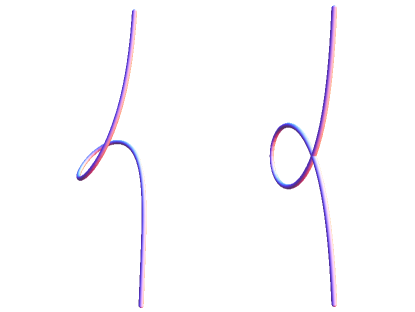
Figure 1: Non-planar (left, $(\epsilon,\tau_{0},t)=(1,0.4,0)$) and planar (right, $(\epsilon,\tau_{0},t)=(1,0,0)$) solitons.

IV Absence of propagation of planar solutions in the PT-symmetric case

In the case of the LIE, the velocity of a Hasimoto soliton is given by $v=2\tau_{0}$ (take $\mu=0$ in Eq. (7)). At $\tau\neq 0$, the solutions are “chiral,” in the sense that their handedness is correlated with the direction of the propagation. A mirror image of a solution propagates in the opposite direction from the original one. If we look at a planar ($\tau=0$) solution at $\mu=0$ (see the right figure of Fig. 1), it just rotates around its axis and cannot convey energy along the vortex. In fact, this is a generic feature. Here, we consider a class of solutions that are asymptotically straight lines, like the Hasimoto solitons. We will now show that these solutions cannot propagate if the equation of motion (EOM) has the PT symmetry. The LIE has this symmetry, while the FME does not.

It suffices to show that, when the solution is planar, the velocity $\dot{\bm{X}}$ is restricted to the direction of $\bm{b}$, since a binomal motion cannot make the soliton propagate along the vortex. Consider a current written in the form

$$\bm{J}=\int ds\,f(\kappa,\tau)\dot{\bm{X}},$$ (21)

where $f(\kappa,\tau)$ is a function of $\kappa$ and $\tau$. The energy current is written in this form. Let us denote the unit vector in the direction of the asymptotic line by $\bm{\ell}$. Since $\bm{\ell}$ is within the plane spanned by $\{\bm{t},\bm{n}\}$ for a planar solution, it is always orthogonal to $\bm{b}$, $\bm{\ell}\cdot\bm{b}=0$. Thus, if $\dot{\bm{X}}\propto\bm{b}$, then $\bm{\ell}\cdot\bm{J}=0$ holds and there is no energy flow in the direction of $\bm{\ell}$.

Let us examine the transformation property of the EOMs. The parity reflection, $\bm{X}\rightarrow-\bm{X}$, acts on the FS system as

$$\{\bm{t},\bm{n},\bm{b},\kappa,\tau\}\longrightarrow\{-\bm{t},-\bm{n},\bm{b},\kappa,-\tau\}.$$ (22)

The binomal vector is parity even, because $\bm{b}=\bm{t}\times\bm{n}$, while the torsion $\tau=(\bm{n}^{\prime}\cdot\bm{b})$ is parity odd. The RHS of the LIE, $\bm{X}^{\prime}\times\bm{X}^{\prime\prime}$, is P-even, while the modification to the LIE in the FME, $\bm{X}^{\prime\prime\prime}+\frac{3}{2}(\bm{X}^{\prime\prime})^{2}\bm{X}^{\prime}$, is P-odd.

A general EOM can be written in the form

$$\dot{\bm{X}}=a(\kappa,\tau)\,\bm{t}+b(\kappa,\tau)\,\bm{n}+c(\kappa,\tau)\,\bm{b}.$$ (23)

From our assumption, the theory has the PT symmetry. The LHS is even under PT. The RHS is T-even, so it has to be P-even. For a planar solution, $\tau=0$, the coefficients in Eq. (23) are all P-even, because $\kappa$ is a P-even quantity. Thus, the coefficients of $\bm{t}$ and $\bm{n}$ have to vanish, $a(\kappa,\tau=0)=b(\kappa,\tau=0)=0$, and $\dot{\bm{X}}\propto\bm{b}$.

The results above can be further generalized. The LIE can be mapped to NLSE, which has an infinite sequence of commuting invariants. Those invariants are the generators of the Hamiltonian flows. Correspondingly, the LIE also has infinitely many commuting Hamiltonian flows Langer and Perline (1991), which are called the LIE hierarchy. The first and second term of the RHS of the FME (4) are the first two Hamiltonian flows,

$$\bm{V}_{0}=\kappa\bm{b},\quad\bm{V}_{1}=\frac{\kappa^{2}}{2}\bm{t}+\kappa^{\prime}\bm{n}+\kappa\tau\bm{b},\quad\cdots$$ (24)

In Ref. Langer and Perline (1991), a recursion operator that successively generates the next flow is constructed,

$$\mathcal{R}\bm{V}\equiv-\mathcal{P}\left[\bm{t}\times\partial_{s}\bm{V}\right],$$ (25)

where $\mathcal{P}$ denotes the reparametrization procedure to keep the arc-length-preserving nature, which is done by adding a tangential term (see also Ref. Holm and Stechmann (2004)). Once we know $\bm{V}_{n}$, we can obtain the next flow by $\bm{V}_{n+1}=\mathcal{R}\bm{V}_{n}$. One can show (see the Supplementary Material) that $\bm{V}_{n}$ is P-even(odd) if $n$ is an even(odd) number. Thus, every EOM with an even $n$ has the PT symmetry, and the solution of the EOM cannot propagate if its planar.

To summarize, we have found a new phenomenon affecting the dynamics of vortex solitons in chirally imbalanced media - the Chiral Propulsion Effect. The CPE refers to an asymmetric energy flow along the vortex filament in the direction determined by the sign of the chirality imbalance. The energy is carried along the vortex by helical excitations analogous to the Hasimoto solitons. We have also found that the growth rate of unstable modes on the helical soliton solution is modified by the chirality of the medium. It is shown that, if the equation of motion respects the PT symmetry, a planar solution cannot transfer energy – this indicates that the existence of the CPE is entirely due to the breaking of parity in the medium.

V Supplementary Material

V.1 Derivation of Eqs. (15) and (16)

The compatibility conditions for the Frenet-Serret frame, $\partial_{s}\partial_{t}\bm{t}=\partial_{t}\partial_{s}\bm{t},\ \partial_{s}\partial_{t}\bm{n}=\partial_{t}\partial_{s}\bm{n},\ \partial_{s}\partial_{t}\bm{b}=\partial_{t}\partial_{s}\bm{b}$, result in the following relations,

$$\partial_{s}\beta=-\alpha\tau+\gamma\kappa,$$ (26)

$$\partial_{t}\begin{pmatrix}\kappa\\ \tau\end{pmatrix}=\begin{pmatrix}0&-\beta\\ \beta&0\end{pmatrix}\begin{pmatrix}\kappa\\ \tau\end{pmatrix}+\partial_{s}\begin{pmatrix}\alpha\\ \gamma\end{pmatrix}.$$ (27)

A generic equation of motion (EOM) of a curve is written in the form

$$\dot{\bm{X}}=a(\kappa,\tau)\,\bm{t}+b(\kappa,\tau)\,\bm{n}+c(\kappa,\tau)\,\bm{b},$$ (28)

where $a(\kappa,\tau),b(\kappa,\tau),c(\kappa,\tau)$ are functions of $\kappa$ and $\tau$. They are related to $\alpha,\beta,\gamma$ in Eq. (14) as

$$\alpha=a\kappa+b^{\prime}-c\tau,\quad\beta=b\tau+c^{\prime},\quad\gamma=\frac{\beta^{\prime}+\tau\alpha}{\kappa},$$ (29)

which can be checked by using the FS formulas. The FME (4) can be written in terms of the FS basis as

$$\dot{\bm{X}}=\frac{\mu}{2}\kappa^{2}\bm{t}+\mu\kappa^{\prime}\bm{n}+\kappa(1+\mu\tau)\bm{b}.$$ (30)

From this expression we can read off $a$, $b$ and $c$ in Eq. (28). By plugging them into Eqs. (29), we obtain the expressions for $\alpha,\beta,\gamma$. Substituting them into Eq. (27), we find the time-evolution equations for $\tau$ and $\kappa$ given by Eq.(15) and Eq.(16).

V.2 The parity symmetry of the higher-order flows of the LIE hierarchy

Here we determine the parity symmetry of the higher-oder flows of the LIE hierarchy, using the recursion operator $\mathcal{R}$. It is shown that $\bm{V}_{n}$ is P-even(odd) if $n$ is an even(odd) number. Suppose $\bm{V}_{n}$ is a flow of a particular parity (even or odd). The $n+1$-th flow can be generated by the operation,

$$\begin{split}\bm{V}_{n+1}&=-\mathcal{R}(\bm{X}^{\prime}\times\partial_{s}\bm{V}_{n})\\ &=-\bm{X}^{\prime}\times\partial_{s}\bm{V}_{n}+\bar{a}(\kappa,\tau)\,\bm{t},\end{split}$$ (31)

where $\bar{a}(\kappa,\tau)\,\bm{t}$ is the added term to keep the arc-length unchanged. The multiplication of $\bm{X}^{\prime}\times\partial_{s}$ changes the parity, because of a factor of $\bm{X}^{\prime}$, and the first term has the opposite parity from $\bm{V}_{n}$. One can see that the reparametrization operation does not change the parity of the flow, as follows. $\bm{V}_{n+1}$ can be written in the form, $\bm{V}_{n+1}=b(\kappa,\tau)\,\bm{n}+c(\kappa,\tau)\,\bm{b}+\bar{a}(\kappa,\tau)\,\bm{t}.$ The arc-length preserving condition, $\bm{t}\cdot\bm{V}_{n+1}^{\prime}=0$, implies that the newly added term has to satisfy $\bar{a}^{\prime}=\kappa b.$ Since $\kappa$ is P-even, $\bar{a}$ has the same parity as $b$, and $\bar{a}\,\bm{t}$ has the same parity as $b\,\bm{n}$. Therefore, $\bm{V}_{n}$ is P-even(odd) if $n$ is an even(odd) number.

References

- Adler (1969) S. L. Adler, Physical Review 177, 2426 (1969).
- Bell and Jackiw (1969) J. S. Bell and R. Jackiw, Il Nuovo Cimento A (1965-1970) 60, 47 (1969).
- Kharzeev (2006) D. Kharzeev, Phys. Lett. B633, 260 (2006), eprint hep-ph/0406125.
- Kharzeev et al. (2008) D. E. Kharzeev, L. D. McLerran, and H. J. Warringa, Nucl.Phys. A803, 227 (2008), eprint 0711.0950.
- Fukushima et al. (2008) K. Fukushima, D. E. Kharzeev, and H. J. Warringa, Phys.Rev. D78, 074033 (2008), eprint 0808.3382.
- Kharzeev et al. (2016) D. E. Kharzeev, J. Liao, S. A. Voloshin, and G. Wang, Prog. Part. Nucl. Phys. 88, 1 (2016), eprint 1511.04050.
- Kharzeev et al. (2013) D. Kharzeev, K. Landsteiner, A. Schmitt, and H.-U. Yee, Lect. Notes Phys. 871, pp.1 (2013).
- Kharzeev and Zhitnitsky (2007) D. Kharzeev and A. Zhitnitsky, Nucl. Phys. A797, 67 (2007), eprint 0706.1026.
- Erdmenger et al. (2009) J. Erdmenger, M. Haack, M. Kaminski, and A. Yarom, JHEP 01, 055 (2009), eprint 0809.2488.
- Banerjee et al. (2011) N. Banerjee, J. Bhattacharya, S. Bhattacharyya, S. Dutta, R. Loganayagam, and P. Surowka, JHEP 01, 094 (2011), eprint 0809.2596.
- Torabian and Yee (2009) M. Torabian and H.-U. Yee, JHEP 08, 020 (2009), eprint 0903.4894.
- Son and Surowka (2009) D. T. Son and P. Surowka, Phys.Rev.Lett. 103, 191601 (2009), eprint 0906.5044.
- Li et al. (2016) Q. Li, D. E. Kharzeev, C. Zhang, Y. Huang, I. Pletikosic, A. V. Fedorov, R. D. Zhong, J. A. Schneeloch, G. D. Gu, and T. Valla, Nature Phys. 12, 550 (2016), eprint 1412.6543.
- Joyce and Shaposhnikov (1997) M. Joyce and M. E. Shaposhnikov, Phys. Rev. Lett. 79, 1193 (1997), eprint astro-ph/9703005.
- Akamatsu and Yamamoto (2013) Y. Akamatsu and N. Yamamoto, Phys. Rev. Lett. 111, 052002 (2013), eprint 1302.2125.
- Avdoshkin et al. (2016) A. Avdoshkin, V. P. Kirilin, A. V. Sadofyev, and V. I. Zakharov, Phys. Lett. B755, 1 (2016), eprint 1402.3587.
- Tashiro et al. (2012) H. Tashiro, T. Vachaspati, and A. Vilenkin, Phys. Rev. D86, 105033 (2012), eprint 1206.5549.
- Hirono et al. (2015) Y. Hirono, D. Kharzeev, and Y. Yin, Phys. Rev. D92, 125031 (2015), eprint 1509.07790.
- Yamamoto (2016) N. Yamamoto, Phys. Rev. D93, 125016 (2016), eprint 1603.08864.
- Hattori et al. (2017) K. Hattori, Y. Hirono, H.-U. Yee, and Y. Yin (2017), eprint 1711.08450.
- Xiong et al. (2015) J. Xiong, S. K. Kushwaha, T. Liang, J. W. Krizan, M. Hirschberger, W. Wang, R. Cava, and N. Ong, Science 350, 413 (2015).
- Li et al. (2015) C.-Z. Li, L.-X. Wang, H. Liu, J. Wang, Z.-M. Liao, and D.-P. Yu, Nature communications 6, 10137 (2015).
- Zhang et al. (2015) C. Zhang, S.-Y. Xu, I. Belopolski, Z. Yuan, Z. Lin, B. Tong, N. Alidoust, C.-C. Lee, S.-M. Huang, H. Lin, et al., arXiv preprint arXiv:1503.02630 (2015).
- Yang et al. (2015a) X. Yang, Y. Liu, Z. Wang, Y. Zheng, and Z.-a. Xu, arXiv preprint arXiv:1506.03190 (2015a).
- Yang et al. (2015b) X. Yang, Y. Li, Z. Wang, Y. Zhen, and Z.-a. Xu, arXiv preprint arXiv:1506.02283 (2015b).
- Koch et al. (2017) V. Koch, S. Schlichting, V. Skokov, P. Sorensen, J. Thomas, S. Voloshin, G. Wang, and H.-U. Yee, Chin. Phys. C41, 072001 (2017), eprint 1608.00982.
- Adamczyk et al. (2017) L. Adamczyk et al. (STAR) (2017), eprint 1701.06657.
- Liang and Wang (2005) Z.-T. Liang and X.-N. Wang, Phys. Rev. Lett. 94, 102301 (2005), [Erratum: Phys. Rev. Lett.96,039901(2006)], eprint nucl-th/0410079.
- Betz et al. (2007) B. Betz, M. Gyulassy, and G. Torrieri, Phys. Rev. C76, 044901 (2007), eprint 0708.0035.
- Becattini et al. (2013) F. Becattini, L. Csernai, and D. J. Wang, Phys. Rev. C88, 034905 (2013), [Erratum: Phys. Rev.C93,no.6,069901(2016)], eprint 1304.4427.
- Becattini et al. (2015) F. Becattini, G. Inghirami, V. Rolando, A. Beraudo, L. Del Zanna, A. De Pace, M. Nardi, G. Pagliara, and V. Chandra, Eur. Phys. J. C75, 406 (2015), eprint 1501.04468.
- Baznat et al. (2016) M. I. Baznat, K. K. Gudima, A. S. Sorin, and O. V. Teryaev, Phys. Rev. C93, 031902 (2016), eprint 1507.04652.
- Pang et al. (2016) L.-G. Pang, H. Petersen, Q. Wang, and X.-N. Wang, Phys. Rev. Lett. 117, 192301 (2016), eprint 1605.04024.
- Deng and Huang (2016) W.-T. Deng and X.-G. Huang, Phys. Rev. C93, 064907 (2016), eprint 1603.06117.
- Jiang et al. (2016) Y. Jiang, Z.-W. Lin, and J. Liao, Phys. Rev. C94, 044910 (2016), eprint 1602.06580.
- Becattini et al. (2017) F. Becattini, I. Karpenko, M. Lisa, I. Upsal, and S. Voloshin, Phys. Rev. C95, 054902 (2017), eprint 1610.02506.
- Karpenko and Becattini (2017) I. Karpenko and F. Becattini, Eur. Phys. J. C77, 213 (2017), eprint 1610.04717.
- Li et al. (2017) H. Li, H. Petersen, L.-G. Pang, Q. Wang, X.-L. Xia, and X.-N. Wang, Nucl. Phys. A967, 772 (2017), eprint 1704.03569.
- Aristova et al. (2016) A. Aristova, D. Frenklakh, A. Gorsky, and D. Kharzeev, JHEP 10, 029 (2016), eprint 1606.05882.
- Saffman (1992) P. G. Saffman, Vortex dynamics (Cambridge university press, 1992).
- Ricca (1991) R. L. Ricca, Nature 352, 561 (1991).
- Vilenkin and Shellard (2000) A. Vilenkin and E. P. S. Shellard, Cosmic strings and other topological defects (Cambridge University Press, 2000).
- Volovik (2009) G. E. Volovik, The universe in a helium droplet, vol. 117 (Oxford University Press, 2009).
- Eto et al. (2013) M. Eto, Y. Hirono, M. Nitta, and S. Yasui, PTEP 2014, 012D01 (2013), eprint 1308.1535.
- Hasimoto (1972) H. Hasimoto, J. Fluid Mech 51, 477 (1972).
- Langer and Perline (1991) J. Langer and R. Perline, Journal of Nonlinear Science 1, 71 (1991).
- Kharzeev (2014) D. E. Kharzeev, Prog. Part. Nucl. Phys. 75, 133 (2014), eprint 1312.3348.
- Kozhevnikov (1999) A. A. Kozhevnikov, Phys. Lett. B461, 256 (1999), eprint hep-ph/9908444.
- Kozhevnikov (2015) A. A. Kozhevnikov, Phys. Lett. B750, 122 (2015), eprint 1509.01937.
- Holm and Stechmann (2004) D. D. Holm and S. N. Stechmann, arXiv preprint nlin/0409040 (2004).
- Fukumoto and Miyazaki (1991) Y. Fukumoto and T. Miyazaki, Journal of fluid mechanics 222, 369 (1991).
- Kambe (2004) T. Kambe, Geometrical theory of dynamical systems and fluid flows, 23 (World Scientific, 2004).
- Hirota (1973) R. Hirota, Journal of Mathematical Physics 14, 805 (1973).
- Ricca (1992) R. L. Ricca, Physics of Fluids A: Fluid Dynamics 4, 938 (1992).
- Da Rios (1906) L. Da Rios, Rend. Circ. Mat. Palermo 22, 117 (1906).
- Kambe and Takao (1971) T. Kambe and T. Takao, Journal of the Physical Society of Japan 31, 591 (1971).
- Betchov (1965) R. Betchov, Journal of Fluid Mechanics 22, 471 (1965).
- Ricca (1996) R. L. Ricca, Fluid Dynamics Research 18, 245 (1996).
- Suzuki et al. (1996) K. Suzuki, T. Ono, and T. Kambe, Phys. Rev. Lett. 77, 1679 (1996), URL https://link.aps.org/doi/10.1103/PhysRevLett.77.1679.
- Ricca (1994) R. L. Ricca, Journal of Fluid Mechanics 273, 241 (1994).
- Thomson (1880) W. Thomson, The London, Edinburgh, and Dublin Philosophical Magazine and Journal of Science 10, 155 (1880).