The Dynamic Geometry of Interaction Machine:
A Token-Guided Graph Rewriter*

Abstract.

In implementing evaluation strategies of the lambda-calculus, both correctness and efficiency of implementation are valid concerns. While the notion of correctness is determined by the evaluation strategy, regarding efficiency there is a larger design space that can be explored, in particular the trade-off between space versus time efficiency. Aiming at a unified framework that would enable the study of this trade-off, we introduce an abstract machine, inspired by Girard’s Geometry of Interaction (GoI), a machine combining token passing and graph rewriting. We show soundness and completeness of our abstract machine, called the Dynamic GoI Machine (DGoIM), with respect to three evaluations: call-by-need, left-to-right call-by-value, and right-to-left call-by-value. Analysing time cost of its execution classifies the machine as “efficient” in Accattoli’s taxonomy of abstract machines.

1. Introduction

The lambda-calculus is a simple yet rich model of computation, relying on a single mechanism to activate a function in computation, beta-reduction, that replaces function parameters with actual input. While in the lambda-calculus itself beta-reduction can be applied in an unrestricted way, it is evaluation strategies that determine the way beta-reduction is applied when the lambda-calculus is used as a programming language. Evaluation strategies often imply how intermediate results are copied, discarded, cached or reused. For example, everything is repeatedly evaluated as many times as requested in the call-by-name strategy. In the call-by-need strategy, once a function requests its input, the input is evaluated and the result is cached for later use. The call-by-value strategy evaluates function input and caches the result even if the function does not require the input.

The implementation of any evaluation strategy must be correct, first of all, i.e. it has to produce results as stipulated by the strategy. Once correctness is assured, the next concern is efficiency. One may prefer better space efficiency, or better time efficiency, and it is well known that one can be traded off for the other. For example, time efficiency can be improved by caching more intermediate results, which increases space cost. Conversely, bounding space requires repeating computations, which adds to the time cost. Whereas correctness is well defined for any evaluation strategy, there is a certain freedom in managing efficiency. The challenge here is how to produce a unified framework which is flexible enough to analyse and guide the choices required by this trade-off. Recent studies by Accattoli et al. [AD16, ABM14, Acc17] clearly establish classes of efficiency for abstract machines that implement a given evaluation strategy. They characterise efficiency by means of the number of beta-reduction applications required by the strategy, and introduce two efficiency classes, namely “efficient” and “reasonable”. This classification of abstract machines gives us a starting point to quantitatively analyse the trade-offs required in an implementation.

1.1. Token-Passing GoI

We employ Girard’s Geometry of Interaction (GoI) [Gir89], a semantics of linear logic proofs, as a framework for studying the trade-off between time and space efficiency. In particular we focus on the token-passing style of GoI, which gives abstract machines for the lambda-calculus, pioneered by Danos and Regnier [DR96] and Mackie [Mac95]. These machines evaluate a term of the lambda-calculus by translating the term to a graph, a network of simple transducers, which executes by passing a data-carrying token around.

Token-passing GoI decomposes higher-order computation into local token actions, or low-level interactions of simple components. It can give strikingly innovative implementation techniques for functional programs, such as Mackie’s Geometry of Implementation compiler [Mac95], Ghica’s Geometry of Synthesis (GoS) high-level synthesis tool [Ghi07], and Schöpp’s resource-aware program transformation to a low-level language [Sch14b]. The interaction-based approach is also convenient for the complexity analysis of programs, e.g. Dal Lago and Schöpp’s IntML type system of logarithmic-space evaluation [DS16], and Dal Lago et al.’s linear dependent type system of polynomial-time evaluation [DG11, DP12].

Fixed-space execution is essential for GoS, since in the case of digital circuits the memory footprint of the program must be known at compile-time, and fixed. Using a restricted version of the call-by-name language Idealised Algol [GS11] not only the graph, but also the token itself can be given a fixed size. Surprisingly, this technique also allows the compilation of recursive programs [GSS11]. The GoS compiler shows both the usefulness of the GoI as a guideline for unconventional compilation and the natural affinity between its space-efficient abstract machine and call-by-name evaluation. The practical considerations match the prior theoretical understanding of this connection [DR96].

The token passed around a graph simulates graph rewriting without actually rewriting, which is in fact an extremal instance of the trade-off we mentioned above. Token-passing GoI keeps the underlying graph fixed and uses the data stored in the token to route it. It therefore favours space efficiency at the cost of time efficiency. The same computation is repeated when, instead, intermediate results could have been cached by saving copies of certain sub-graphs representing values.

1.2. Interleaving Token Passing with Graph Rewriting

Our intention is to lift the token-passing GoI to a framework to analyse the trade-off of efficiency, by strategically interleaving it with graph rewriting. We present the framework as an abstract machine that interleaves token passing with graph rewriting. The machine, called the Dynamic GoI Machine (DGoIM), is defined as a state transition system with transitions for token passing as well as transitions for graph rewriting. The key idea is that the token holds control over graph rewriting, by visiting redexes and triggering the rewrite transitions.

Graph rewriting offers fine control over caching and sharing intermediate results. Through graph rewriting, the DGoIM can reduce sub-graphs visited by the token, avoiding repeated token actions and improving time efficiency. However, fetching cached results can increase the size of the graph. In short, introduction of graph rewriting sacrifices space while favouring time efficiency. We expect the flexibility given by a fine-grained control over interleaving will enable a careful balance between space and time efficiency.

As a first step in our exploration of the flexibility of this machine, we consider the two extremal cases of interleaving. The first extremal case is “passes-only”, in which the DGoIM never triggers graph rewriting, yielding an ordinary token-passing abstract machine. As a typical example, the $\lambda$-term $(\lambda{x}.t)\,u$ is evaluated like this:

1. A token enters the graph on the left at the bottom open edge.

2. A token visits and goes through the left sub-graph $\lambda{x}.t$.

3. Whenever a token detects an occurrence of the variable $x$ in $t$, it traverses the right sub-graph $u$, then returns carrying information about the resulting value of $u$.

4. A token finally exits the graph at the bottom open edge.

Step 3 is repeated whenever the argument $u$ needs to be re-evaluated. This passes-only strategy of interleaving corresponds to call-by-name evaluation.

The other extreme is “rewrites-first”, in which the DGoIM interleaves token passing with as much, and as early, graph rewriting as possible, guided by the token. This corresponds to both call-by-value and call-by-need evaluations, with different trajectories of the token. In the case of left-to-right call-by-value, the token enters the graph from the bottom, traverses the left-hand-side sub-graph, which happens to be already a value, then visits the sub-graph $u$ even before the bound variable $x$ is used in a call. The token causes rewrites while traversing the sub-graph $u$, and when it exits, it leaves behind a graph corresponding to a value $v$ such that $u$ reduces to $v$. For right-to-left call-by-value, the token visits the sub-graph $u$ straightaway after entering the whole graph, reduces the sub-graph $u$, to the graph of the value $v$, and visits the left-hand-side sub-graph. The difference with call-by-need is that the token visits and reduces the sub-graph $u$ only when the variable $x$ is encountered in $\lambda{x}.t$.

In our framework, all these three evaluations involve similar tactics for caching intermediate results. Different trajectories of the token realise their only difference, which is the timing of cache creation. Cached values are fetched in the same way: namely, if repeated evaluation is required, then the sub-graph corresponding now to the value $v$ is copied. One copy can be further rewritten, if needed, while the original is kept for later reference.

1.3. Contributions

This work presents a token-guided graph-rewriting abstract machine for call-by-need, left-to-right call-by-value, and right-to-left call-by-value evaluations. The abstract machine is given by the rewrites-first strategy of the DGoIM, which turns out to be as natural as the passes-only strategy for call-by-name evaluation. It switches the evaluations, by simply having different nodes that correspond to the three different evaluations, rather than modifying the behaviour of a single node to suite different evaluation demands. This can be seen as a case study illustrating the flexibility of the DGoIM, which is achieved through controlled interleaving of rewriting and token-passing, and through changing graph representations of terms.

We prove the soundness and completeness of the extended machine with respect to the three evaluations separately, using a “sub-machine” semantics, where the word “sub” indicates both a focus on substitution and its status as an intermediate representation. The sub-machine semantics is based on Sinot’s “token-passing” semantics [Sin05, Sin06] that makes explicit the two main tasks of abstract machines: searching redexes and substituting variables.

The time-cost analysis classifies the machine as “efficient” in Accattoli’s taxonomy of abstract machines [Acc17]. We follow Accattoli et al.’s general methodology for quantitative analysis of abstract machines [ABM14, Acc17], however the method cannot be used “off the shelf”. Our machine is a more refined transition system with more transition steps, and therefore does not satisfy one of their assumptions [Acc17, Sec. 3], which requires one-to-one correspondence of transition steps. We overcome this technical difficulty by building a weak simulation of the sub-machine semantics, which is also used in the proof of soundness and completeness. The sub-machine semantics resembles Danvy and Zerny’s storeless abstract machine [DZ13], to which the general recipe of cost analysis does apply.

Finally, an on-line visualiser is implemented, in which our machine can be executed on arbitrary closed (untyped) lambda-terms. The visualiser also supports an existing abstract machine based on the token-passing GoI, which will be discussed later, to illustrate various resource usage of abstract machines.

The rest of the paper is organised as follows. We present the sub-machine semantics in Sec. 2, and introduce the DGoIM with the rewrites-first strategy in Sec. 3. In Sec. 4, we show how the DGoIM implements the three evaluation strategies via translation of terms into graphs, and establish a weak simulation of the sub-machine semantics by the DGoIM. The simulation result is used to prove soundness and completeness of the DGoIM, and to analyse its time cost, in Sec. 5. We compare our graph-rewriting approach to improve time efficiency of token-passing GoI, with another approach from the literature, namely “jumping” approach, in Sec. 6. We discuss related conventional abstract machines in Sec. 7.

2. A Term Calculus with Sub-Machine Semantics

We use an untyped term calculus that accommodates three evaluation strategies of the lambda-calculus, by dedicated constructors for function application: namely, $\mathbin{@}$ (call-by-need), $\mathbin{\overrightarrow{@}}$ (left-to-right call-by-value) and $\mathbin{\overleftarrow{@}}$ (right-to-left call-by-value). The term calculus uses all strategies so that we do not have to present three almost identical calculi. Nevertheless, we are not interested in their interaction but in each strategy separately. In the rest of the paper, we therefore assume that each term contains function applications of a single strategy. As shown in the top of Fig. 1, the calculus accommodates explicit substitutions $[x\leftarrow u]$. A term with no explicit substitutions is said to be “pure”.

The sub-machine semantics is used to establish the soundness of the graph-rewriting abstract machine. It imitates an abstract machine, by having the following two features. Firstly, it extends conventional reduction semantics with reduction steps that explicitly search for a redex, following the style of Sinot’s “token-passing semantics” [Sin05, Sin06]. Secondly, it decomposes the meta-level substitution into on-demand linear substitution, using explicit substitutions, as the linear substitution calculus does [AK10]. The sub-machine semantics also resembles a storeless abstract machine (e.g. [DMMZ12, Fig. 8]). However the semantics is still too “abstract” to be considered an abstract machine, in the sense that it works modulo alpha-equivalence to avoid variable captures.

Fig. 1 defines the sub-machine semantics of our calculus. It is given by labelled relations between enriched terms $E\langle\llparenthesis t\rrparenthesis\rangle$. In an enriched term $E\langle\llparenthesis t\rrparenthesis\rangle$, a sub-term $t$ is not plugged directly into the evaluation context, but into a “window” $\llparenthesis\cdot\rrparenthesis$ which makes it syntactically obvious where the reduction context is situated. Forgetting the window turns an enriched term into an ordinary term. Basic rules $\mapsto$ are labelled with $\beta$, $\sigma$ or $\epsilon$. The basic rules (2), (5) and (8), labelled with $\beta$, apply beta-reduction and delay substitution of a bound variable. Substitution is done one by one, and on demand, by the basic rule (10) with label $\sigma$. Each application of the basic rule (10) replaces exactly one bound variable with a value, and keeps a copy of the value for later use. All other basic rules, with label $\epsilon$, search for a redex by moving the window without changing the underlying term. Finally, reduction is defined by congruence of basic rules with respect to evaluation contexts, and labelled accordingly. Any basic rules and reductions are indeed between enriched terms, because the window $\llparenthesis\cdot\rrparenthesis$ is never duplicated or discarded. They are also deterministic.

Terms $$t \,::=\,x\mid\lambda{x}.t\mid t\mathbin{@}t\mid t\mathbin{\overrightarrow{@}}t\mid t\mathbin{\overleftarrow{@}}t\mid t[x\leftarrow t]$$

Values $$v \,::=\,\lambda{x}.t$$

Answer contexts $$A \,::=\,\langle\cdot\rangle\mid A[x\leftarrow t]$$

Evaluation contexts $$E \,::=\,\langle\cdot\rangle\mid E[x\leftarrow t]\mid E\langle x\rangle[x\leftarrow E]$$

$$\quad\enspace\mid E\mathbin{@}t\mid E\mathbin{\overrightarrow{@}}t\mid A\langle v\rangle\mathbin{\overrightarrow{@}}E\mid t\mathbin{\overleftarrow{@}}E\mid E\mathbin{\overleftarrow{@}}A\langle v\rangle$$

$$\text{Basic rules }\mapsto_{\beta},\mapsto_{\sigma},\mapsto_{\epsilon}: \llparenthesis t\mathbin{@}u\rrparenthesis \mapsto_{\epsilon}\llparenthesis t\rrparenthesis\mathbin{@}u$$ (1)

$$A\langle\llparenthesis\lambda{x}.t\rrparenthesis\rangle\mathbin{@}u \mapsto_{\beta}A\langle\llparenthesis t\rrparenthesis[x\leftarrow u]\rangle$$ (2)

$$\llparenthesis t\mathbin{\overrightarrow{@}}u\rrparenthesis \mapsto_{\epsilon}\llparenthesis t\rrparenthesis\mathbin{\overrightarrow{@}}u$$ (3)

$$A\langle\llparenthesis\lambda{x}.t\rrparenthesis\rangle\mathbin{\overrightarrow{@}}u \mapsto_{\epsilon}A\langle\lambda{x}.t\rangle\mathbin{\overrightarrow{@}}\llparenthesis u\rrparenthesis$$ (4)

$$A\langle\lambda{x}.t\rangle\mathbin{\overrightarrow{@}}A^{\prime}\langle\llparenthesis v\rrparenthesis\rangle \mapsto_{\beta}A\langle\llparenthesis t\rrparenthesis[x\leftarrow A^{\prime}\langle v\rangle]\rangle$$ (5)

$$\llparenthesis t\mathbin{\overleftarrow{@}}u\rrparenthesis \mapsto_{\epsilon}t\mathbin{\overleftarrow{@}}\llparenthesis u\rrparenthesis$$ (6)

$$t\mathbin{\overleftarrow{@}}A\langle\llparenthesis v\rrparenthesis\rangle \mapsto_{\epsilon}\llparenthesis t\rrparenthesis\mathbin{\overleftarrow{@}}A\langle v\rangle$$ (7)

$$A\langle\llparenthesis\lambda{x}.t\rrparenthesis\rangle\mathbin{\overleftarrow{@}}A^{\prime}\langle v\rangle \mapsto_{\beta}A\langle\llparenthesis t\rrparenthesis[x\leftarrow A^{\prime}\langle v\rangle]\rangle$$ (8)

$$E\langle\llparenthesis x\rrparenthesis\rangle[x\leftarrow A\langle u\rangle] \mapsto_{\epsilon}E\langle x\rangle[x\leftarrow A\langle\llparenthesis u\rrparenthesis\rangle]$$

($$u A^{\prime}\langle t^{\prime}\rangle$$ is not in the form of ) (9)

$$E\langle x\rangle[x\leftarrow A\langle\llparenthesis v\rrparenthesis\rangle] \mapsto_{\sigma}A\langle E\langle\llparenthesis v\rrparenthesis\rangle[x\leftarrow v]\rangle$$ (10)

$$\text{Reductions }\multimap_{\beta},\multimap_{\sigma},\multimap_{\epsilon}: E\langle\tilde{t}\rangle\multimap_{\chi}E\langle\tilde{u}\rangle\tilde{t}\mapsto_{\chi}\tilde{u}$$

Figure 1. ”Sub-Machine” Operational Semantics

Call-by-need evaluation:

$\begin{aligned} {\color[rgb]{0,0,0}\llparenthesis(\lambda{x}.x)\mathbin{@}((\lambda{y}.y)\mathbin{@}(\lambda{z}.z))\rrparenthesis}&{\color[rgb]{.5,.5,.5}\multimap_{\epsilon}\llparenthesis\lambda{x}.x\rrparenthesis\mathbin{@}((\lambda{y}.y)\mathbin{@}(\lambda{z}.z))}\\ &{\color[rgb]{0,0,0}\multimap_{\beta}\llparenthesis x\rrparenthesis[x\leftarrow(\lambda{y}.y)\mathbin{@}(\lambda{z}.z)]}\\ &{\color[rgb]{.5,.5,.5}\multimap_{\epsilon}x[x\leftarrow\llparenthesis(\lambda{y}.y)\mathbin{@}(\lambda{z}.z)\rrparenthesis]}\\ &{\color[rgb]{.5,.5,.5}\multimap_{\epsilon}x[x\leftarrow\llparenthesis\lambda{y}.y\rrparenthesis\mathbin{@}(\lambda{z}.z)]}\\ &{\color[rgb]{0,0,0}\multimap_{\beta}x[x\leftarrow\llparenthesis y\rrparenthesis[y\leftarrow\lambda{z}.z]]}\\ &{\color[rgb]{.5,.5,.5}\multimap_{\epsilon}x[x\leftarrow y[y\leftarrow\llparenthesis\lambda{z}.z\rrparenthesis]]}\\ &{\color[rgb]{0,0,0}\multimap_{\sigma}x[x\leftarrow\llparenthesis\lambda{z}.z\rrparenthesis[y\leftarrow\lambda{z}.z]]}\\ &{\color[rgb]{0,0,0}\multimap_{\sigma}\llparenthesis\lambda{z}.z\rrparenthesis[x\leftarrow\lambda{z}.z][y\leftarrow\lambda{z}.z]}\end{aligned}$

Call-by-value evaluations:

$\begin{aligned} &{\color[rgb]{0,0,0}\llparenthesis(\lambda{x}.x)\mathbin{\overrightarrow{@}}((\lambda{y}.y)\mathbin{\overrightarrow{@}}(\lambda{z}.z))\rrparenthesis}\\ &{\color[rgb]{.5,.5,.5}\multimap_{\epsilon}\llparenthesis\lambda{x}.x\rrparenthesis\mathbin{\overrightarrow{@}}((\lambda{y}.y)\mathbin{\overrightarrow{@}}(\lambda{z}.z))}\\ &{\color[rgb]{.5,.5,.5}\multimap_{\epsilon}\lambda{x}.x\mathbin{\overrightarrow{@}}\llparenthesis(\lambda{y}.y)\mathbin{\overrightarrow{@}}(\lambda{z}.z)\rrparenthesis}\\ &{\color[rgb]{.5,.5,.5}\multimap_{\epsilon}\lambda{x}.x\mathbin{\overrightarrow{@}}(\llparenthesis\lambda{y}.y\rrparenthesis\mathbin{\overrightarrow{@}}(\lambda{z}.z))}\\ &{\color[rgb]{.5,.5,.5}\multimap_{\epsilon}\lambda{x}.x\mathbin{\overrightarrow{@}}((\lambda{y}.y)\mathbin{\overrightarrow{@}}\llparenthesis\lambda{z}.z\rrparenthesis)}\\ &{\color[rgb]{0,0,0}\multimap_{\beta}\lambda{x}.x\mathbin{\overrightarrow{@}}(\llparenthesis y\rrparenthesis[y\leftarrow\lambda{z}.z])}\\ &{\color[rgb]{.5,.5,.5}\multimap_{\epsilon}\lambda{x}.x\mathbin{\overrightarrow{@}}(y[y\leftarrow\llparenthesis\lambda{z}.z\rrparenthesis])}\\ &{\color[rgb]{0,0,0}\multimap_{\sigma}\lambda{x}.x\mathbin{\overrightarrow{@}}(\llparenthesis\lambda{z}.z\rrparenthesis[y\leftarrow\lambda{z}.z])}\\ &{\color[rgb]{0,0,0}\multimap_{\beta}\llparenthesis x\rrparenthesis[x\leftarrow(\lambda{z}.z)[y\leftarrow\lambda{z}.z]]}\\ &{\color[rgb]{.5,.5,.5}\multimap_{\epsilon}x[x\leftarrow\llparenthesis\lambda{z}.z\rrparenthesis[y\leftarrow\lambda{z}.z]]}\\ &{\color[rgb]{0,0,0}\multimap_{\sigma}\llparenthesis\lambda{z}.z\rrparenthesis[x\leftarrow\lambda{z}.z][y\leftarrow\lambda{z}.z]}\\ \end{aligned}$			$\begin{aligned} &{\color[rgb]{0,0,0}\llparenthesis(\lambda{x}.x)\mathbin{\overleftarrow{@}}((\lambda{y}.y)\mathbin{\overleftarrow{@}}(\lambda{z}.z))\rrparenthesis}\\ &{\color[rgb]{.5,.5,.5}\multimap_{\epsilon}\lambda{x}.x\mathbin{\overleftarrow{@}}\llparenthesis(\lambda{y}.y)\mathbin{\overleftarrow{@}}(\lambda{z}.z)\rrparenthesis}\\ &{\color[rgb]{.5,.5,.5}\multimap_{\epsilon}\lambda{x}.x\mathbin{\overleftarrow{@}}((\lambda{y}.y)\mathbin{\overleftarrow{@}}\llparenthesis\lambda{z}.z\rrparenthesis)}\\ &{\color[rgb]{.5,.5,.5}\multimap_{\epsilon}\lambda{x}.x\mathbin{\overleftarrow{@}}(\llparenthesis\lambda{y}.y\rrparenthesis\mathbin{\overleftarrow{@}}(\lambda{z}.z))}\\ &{\color[rgb]{0,0,0}\multimap_{\beta}\lambda{x}.x\mathbin{\overleftarrow{@}}(\llparenthesis y\rrparenthesis[y\leftarrow\lambda{z}.z])}\\ &{\color[rgb]{.5,.5,.5}\multimap_{\epsilon}\lambda{x}.x\mathbin{\overleftarrow{@}}(y[y\leftarrow\llparenthesis\lambda{z}.z\rrparenthesis])}\\ &{\color[rgb]{0,0,0}\multimap_{\sigma}\lambda{x}.x\mathbin{\overleftarrow{@}}(\llparenthesis\lambda{z}.z\rrparenthesis[y\leftarrow\lambda{z}.z])}\\ &{\color[rgb]{.5,.5,.5}\multimap_{\epsilon}\llparenthesis\lambda{x}.x\rrparenthesis\mathbin{\overleftarrow{@}}((\lambda{z}.z)[y\leftarrow\lambda{z}.z])}\\ &{\color[rgb]{0,0,0}\multimap_{\beta}\llparenthesis x\rrparenthesis[x\leftarrow(\lambda{z}.z)[y\leftarrow\lambda{z}.z]]}\\ &{\color[rgb]{.5,.5,.5}\multimap_{\epsilon}x[x\leftarrow\llparenthesis\lambda{z}.z\rrparenthesis[y\leftarrow\lambda{z}.z]]}\\ &{\color[rgb]{0,0,0}\multimap_{\sigma}\llparenthesis\lambda{z}.z\rrparenthesis[x\leftarrow\lambda{z}.z][y\leftarrow\lambda{z}.z]}\\ \end{aligned}$

Figure 2. Evaluations of $(\lambda{x}.x)\,((\lambda{y}.y)\,(\lambda{z}.z))$

An evaluation of a pure term $t$ (i.e. a term with no explicit substitution) is a sequence of reductions starting from $\langle\llparenthesis t\rrparenthesis\rangle$, which is simply $\llparenthesis t\rrparenthesis$. Fig. 2 shows evaluations of a pure term $(\lambda{x}.x)\,((\lambda{y}.y)\,(\lambda{z}.z))$ in the three evaluation strategies. Reductions labelled with $\beta$ and $\sigma$, which change an underlying term, are highlighted in black. All three evaluations involve two beta-reductions, which apply $\lambda{x}.x$ and $\lambda{y}.y$ to an argument. Application of $\lambda{x}.x$ comes first in the call-by-need evaluation, and delayed application of $\lambda{y}.y$ happens inside an explicit substitution. On the other hand, in two call-by-value evaluations, application of $\lambda{y}.y$ comes first, and no reduction happens inside an explicit substitution. The two call-by-value evaluations differ only in the way the window is moved around function application.

The following lemma enables us to follow the use of sub-terms of the initial term $t$ during the evaluation.

Lemma 1.

For any evaluation $\llparenthesis t\rrparenthesis\multimap^{*}E^{\prime}\langle\llparenthesis t^{\prime}\rrparenthesis\rangle$ starting from a pure closed term $t$, the term $t^{\prime}$ is a sub-term of $t$. Moreover, the evaluation context $E^{\prime}$ is given by the following restricted grammar:

$$\overline{A} \,::=\,\langle\cdot\rangle\mid\overline{A}[x\leftarrow\overline{A}\langle u\rangle],$$

$$\overline{E} \,::=\,\langle\cdot\rangle\mid\overline{E}[x\leftarrow\overline{A}\langle u\rangle]\mid\overline{E}\langle x\rangle[x\leftarrow\overline{E}]$$

$$\quad\enspace\mid\overline{E}\mathbin{@}u\mid\overline{E}\mathbin{\overrightarrow{@}}u\mid\overline{A}\langle v\rangle\mathbin{\overrightarrow{@}}\overline{E}\mid u\mathbin{\overleftarrow{@}}\overline{E}\mid\overline{E}\mathbin{\overleftarrow{@}}\overline{A}\langle v\rangle$$

where $u$ and $v$ are sub-terms of $t$, and $v$ is additionally a value.

Proof 2.1 (Proof outline).

The proof is by induction on the length $k$ of the evaluation $\llparenthesis t\rrparenthesis\multimap^{k}E^{\prime}\langle\llparenthesis t^{\prime}\rrparenthesis\rangle$. In the base case, where $k=0$, we have $\overline{E}=\langle\cdot\rangle$ and $t^{\prime}=t$. The inductive case, where $k>0$, is proved by inspecting a basic rule used in the last reduction of the evaluation. In the case of the basic rule (9), the last reduction is in the form of $E_{0}\langle E\langle\llparenthesis x\rrparenthesis\rangle[x\leftarrow A\langle u\rangle]\rangle\multimap_{\epsilon}E_{0}\langle E\langle x\rangle[x\leftarrow A\langle\llparenthesis u\rrparenthesis\rangle]\rangle$ where $u$ is not in the form of $A^{\prime\prime}\langle t^{\prime\prime}\rangle$. By induction hypothesis, $E_{0}\langle E\langle\rangle[x\leftarrow A\langle u\rangle]\rangle$ follows the restricted grammar, and in particular, $A\langle u\rangle$ can be decomposed into a restricted answer context and a sub-term of $t$. Because a sub-term of $t$ is also pure, it follows that $A$ itself is a restricted answer context and $u$ is a sub-term of $t$.

3. The Token-Guided Graph-Rewriting Machine

In the initial presentation of this work [MG17a], we used proof nets of the multiplicative and exponential fragment of linear logic [Gir87] to implement the call-by-need evaluation strategy. Aiming additionally at two call-by-value evaluation strategies, we here use graphs that are closer to syntax trees but are still augmented with the $\mathop{!}$-box structure taken from proof nets. Moving towards syntax trees allows us to accommodate two call-by-value evaluations in a uniform way. The $\mathop{!}$-box structures specify duplicable sub-graphs, and help time-cost analysis of implementations.

3.1. Graphs with Interface

We use directed graphs, whose nodes are classified into proper nodes and link nodes. Link nodes are required to meet the following conditions.

• For each edge, at least one of its two endpoints is a link node.

• Each link node is a source of at most one edge, and a target of at most one edge.

In particular, a link node is called input if it is not a target of any edge, and output if it is not a source of any edge. An interface of a graph is given by the set of all inputs and the set of all outputs. When a graph $G$ has $n$ input link nodes and $m$ output link nodes, we sometimes write $G(n,m)$ to emphasise its interface. If a graph has exactly one input, we refer to the input link node as “root”.

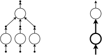
Figure 3. Full (Left) and Simplified (Right) Representation of a Graph $G(3,1)$

An example graph $G(3,1)$ is shown on the left in Fig. 3. It has four proper nodes depicted by circles, and seven link nodes depicted by bullets. Its three inputs are placed at the bottom and one output is at the top. Shown on the right in Fig. 3 is a simplified version of the representation. We use the following simplification scheme: not drawing link nodes explicitly (unless necessary), and using a bold-stroke arrow (resp. circle) to represent a bunch of parallel edges (resp. proper nodes).

The idea of using link nodes, as distinguished from proper nodes, comes from a graphical formalisation of string diagrams [Kis12]. String diagrams consist of “boxes” that are connected to each other by “wires”, and may have dangling or looping wires. In the formalisation, boxes are modelled by “box-vertices” (corresponding to proper nodes in our case), and wires are modelled by consecutive edges connected via “wire-vertices” (corresponding to link nodes in our case). It is link nodes that allow dangling or looping wires to be properly modelled. The segmentation of wires into edges can introduce an arbitrary number of consecutive link nodes, however these consecutive link nodes are identified by the notion of “wire homeomorphism”. We will later discuss these consecutive link nodes, from the perspective of the graph-rewriting machine. From now on we simply call a proper node “node”, and a link node “link”.

Finally, an operation $\circ_{n,m}$ on graphs, parametrised by natural numbers $n$ and $m$, is defined as follows:

$$G\circ_{n,m}H:=\parbox[c]{142.26378pt}{\includegraphics[scale={0.9}]{fig.draw.io/figCrossComposition}}.$$

In the sequel, we omit the parameters $n,m$ and simply write $\circ$.

3.2. Node Labels and $\mathop{!}$-Boxes

We use the following set $\mathcal{L}$ to label nodes:

$$\mathcal{L}=\{\lambda,\mathbin{@},\mathbin{\overrightarrow{@}},\mathbin{\overleftarrow{@}},\mathop{!},\wn,\mathit{D}\}\cup\{\mathit{C}_{n}\mid\text{$n$: a natural number}\}.$$

A node labelled with $X\in\mathcal{L}$ is called an “$X$-node”. The first four labels correspond to the constructors of the calculus presented in Sec. 2, namely $\lambda$ (abstraction), $\mathbin{@}$ (call-by-need application), $\mathbin{\overrightarrow{@}}$ (left-to-right call-by-value application) and $\mathbin{\overleftarrow{@}}$ (right-to-left call-by-value application). These three application nodes are the novelty of this work. The token, travelling in a graph, reacts to these nodes in different ways, and hence implements different evaluation orders. We believe that this is a more extensible way to accommodate different evaluation orders, than to let the token react to the same node in different ways depending on situation.

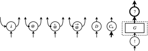
Figure 4. Generators of Graphs

The other labels, namely $\mathop{!}$, $\wn$, $\mathit{D}$ and $\mathit{C}_{n}$ for any natural number $n$, are used in the management of copying sub-graphs. These are inspired by proof nets of the multiplicative and exponential fragment of linear logic [Gir87], and $\mathit{C}_{n}$-nodes generalise the standard binary contraction and subsume weakening.

We use the generators in Fig. 4 to build labelled graphs. Most generators are given by a graph that consists of one node and a fixed number of adjacent links. The number of input/output and incoming/outgoing edges for the node is determined by the label, as indicated in the figure; in particular, a label $\mathit{C}_{n}$ indicates $n$ inputs and $n$ incoming edges. We distinguish two outputs of an application node ($\mathbin{@}$, $\mathbin{\overrightarrow{@}}$ or $\mathbin{\overleftarrow{@}}$), calling one “function output” and the other “argument output” (cf. [AG09]). A bullet $\bullet$ in the figure specifies a function output.

The last generator in Fig. 4 turns a graph $G(1,m)$ into a sub-graph (“$\mathop{!}$-box”), by connecting it to one $\mathop{!}$-node (“principal door”) and $m$ $\wn$-nodes (“auxiliary doors”). This $\mathop{!}$-box structure is indicated by a dashed box in the figure. The $\mathop{!}$-box structure, taken from proof nets, assists the management of duplication of sub-graphs by specifying those that can be copied.

3.3. Graph States and Transitions

We define a graph-rewriting abstract machine as a labelled transition system between graph states. [Graph states] A graph state $((G(1,0),e),\delta)$ is formed of a graph $G(1,0)$ with its distinguished link $e$, and token data $\delta=(d,f,S,B)$ that consists of:

• a direction defined by $d::=\mathord{\uparrow}\mid\mathord{\downarrow}$,

• a rewrite flag defined by $f::=\square\mid\lambda\mid\mathop{!}$,

• a computation stack defined by $S::=\square\mid\star:S\mid\lambda:S\mid@:S$, and

• a box stack defined by $B::=\square\mid\star:B\mid\mathop{!}:B\mid\diamond:B\mid e^{\prime}:B$, where $e^{\prime}$ is any link of the graph $G$.

The distinguished link $e$ is called the “position” of the token. The token reacts to a node in a graph using its data, which determines its path. Given a graph $G$ with root $e_{0}$, the initial state $\mathit{Init}(G)$ on it is given by $((G,e_{0}),(\mathord{\uparrow},\square,\square,\star:\square))$, and the final state $\mathit{Final}(G)$ on it is given by $((G,e_{0}),(\mathord{\downarrow},\square,\square,\mathop{!}:\square))$. An execution on a graph $G$ is a sequence of transitions starting from the initial state $\mathit{Init}(G)$.

Each transition $((G,e),\delta)\to_{\chi}((G^{\prime},e^{\prime}),\delta^{\prime})$ between graph states is labelled by either $\beta$, $\sigma$ or $\epsilon$. Transitions are deterministic, and classified into pass transitions that search for redexes and trigger rewriting, and rewrite transitions that actually rewrite a graph as soon as a redex is found.

A pass transition $((G\circ H,e),(d,\square,S,B))\to_{\epsilon}((G\circ H,e^{\prime}),(d^{\prime},f^{\prime},S^{\prime},B^{\prime}))$, always labelled with $\epsilon$, applies to a state whose rewrite flag is $\square$. The graph $H$ contains only one node, and the positions $e$ and $e^{\prime}$ are an input or an output of the node. The transition simply moves the token over the node, and updates its data by modifying the top elements of stacks, while keeping an underlying graph unchanged. When the token passes a $\lambda$-node or a $\mathop{!}$-node, a rewrite flag is changed to $\lambda$ or $\mathop{!}$, which triggers a rewrite transition. Fig. 5 defines pass transitions, by showing the single-node graph $H$, token positions and data, omitting the graph $G$. The position of the token is drawn as a black triangle, pointing towards the direction of the token. The pass transition over a $\mathit{C}_{n}$-node, where $n$ is positive, pushes the old position $e$ to a box stack. The link $e$ is drawn as a bullet.

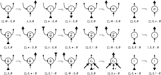
where $X\neq\star$.

Figure 5. Pass Transitions

The way the token reacts to application nodes ($\mathbin{@}$, $\mathbin{\overrightarrow{@}}$ and $\mathbin{\overleftarrow{@}}$) corresponds to the way the window $\llparenthesis\cdot\rrparenthesis$ moves in evaluating these function applications in the sub-machine semantics (Fig. 1). When the token moves on to the composition output of an application node, the top element of a computational stack is either $@$ or $\star$. The element $\star$ makes the token return from a $\lambda$-node, which corresponds to reducing the function part of application to a value (i.e. abstraction). The element $@$ lets the token proceed at a $\lambda$-node, raises the rewrite flag $\lambda$, and hence triggers a rewrite transition that corresponds to beta-reduction. The call-by-value application nodes ($\mathbin{\overrightarrow{@}}$ and $\mathbin{\overleftarrow{@}}$) send the token to their argument output, pushing the element $\star$ to a box stack. This makes the token bounce at a $\mathop{!}$-node and return to the application node, which corresponds to evaluating the argument part of function application to a value. Finally, pass transitions through $\mathit{D}$-nodes, $\mathit{C}_{n}$-nodes and $\mathop{!}$-nodes prepare copying of values, and eventually raise the rewrite flag $\mathop{!}$ that triggers on-demand duplication.

A rewrite transition $((G\circ H,e),(d,f,S,B))\to_{\chi}((G\circ H^{\prime},e^{\prime}),(d^{\prime},f^{\prime},S,B^{\prime}))$, labelled with $\chi\in\{\beta,\sigma,\epsilon\}$, applies to a state whose rewrite flag is either $\lambda$ or $\mathop{!}$. It replaces the sub-graph $H$ (“redex”) with the graph $H^{\prime}$ of the same interface. The position $e$ that belongs to $H$ is changed to the position $e^{\prime}$ that belongs to $H^{\prime}$. The transition may pop an element from a box stack. Fig. 6 defines rewrite transitions, by showing the sub-graphs $H$ and $H^{\prime}$, as well as token positions and data, omitting the graph $G$. Before we go through each rewrite transition, we note that rewrite transitions are not exhaustive in general, as a graph may not match a redex even though a rewrite flag is raised. However we will see that there is no failure of transitions in implementing the term calculus.

where $Y\in\mathcal{L}$, $Z\in\mathcal{L}$, $\$\in\{\mathbin{@},\mathbin{\overrightarrow{@}},\mathbin{\overleftarrow{@}}\}$, and $G(1,n)$ is any graph.

Figure 6. Rewrite Transitions

The first rewrite transition in Fig. 6, with label $\beta$, occurs when a rewrite flag is $\lambda$. It implements beta-reduction by eliminating a pair of an abstraction node ($\lambda$) and an application node ($\$\in\{\mathbin{@},\mathbin{\overrightarrow{@}},\mathbin{\overleftarrow{@}}\}$ in the figure). Outputs of the $\lambda$-node are required to be connected to arbitrary nodes (labelled with $Y$ and $Z$ in the figure), so that edges between links are not introduced. The other rewrite transitions are for the rewrite flag $\mathop{!}$, and they together realise the copying process of a sub-graph (namely a $\mathop{!}$-box). The second rewrite transition in Fig. 6, labelled with $\epsilon$, finishes off each copying process by eliminating all doors of the $\mathop{!}$-box $G$. It replaces the interface of $G$ with output links of the auxiliary doors and the input link of the $\mathit{D}$-node, which is the new position of the token, and pops the top element $\diamond$ of a box stack. Again, no edge between links are introduced.

The last rewrite transition in the figure, with label $\sigma$, actually copies a $\mathop{!}$-box. It requires the top element $e$ of the old box stack to be one of input links of the $\mathit{C}_{k+1}$-node (where $k$ is a natural number). The link $e$ is popped from the box stack and becomes the new position of the token, and the $\mathit{C}_{k+1}$-node becomes a $\mathit{C}_{k}$-node by keeping all the inputs except for the link $e$. The sub-graph $H(n+m,l)$ must consist of $l$ parallel $\mathit{C}$-nodes that altogether have $n+m$ inputs. Among these inputs, $n$ must be connected to auxiliary doors of the $\mathop{!}$-box $G(1,n)$, and $m$ must be connected to nodes that are not in the redex. The sub-graph $H(n+m,l)$ is turned into $H^{\prime}(2n+m,l)$ by introducing $n$ inputs to these $\mathit{C}$-nodes as follows: if an auxiliary door of the $\mathop{!}$-box $G$ is connected to a $\mathit{C}$-node in $H$, two copies of the auxiliary door are both connected to the corresponding $\mathit{C}$-node in $H^{\prime}$. Therefore the two sub-graphs consist of the same number $l$ of $\mathit{C}$-nodes, whose indegrees are possibly increased. The $m$ inputs, connected to nodes outside a redex, are kept unchanged. Fig. 7 shows an example where copying of the graph $G(1,3)$ turns the graph $H(5,2)$ into $H^{\prime}(8,2)$.

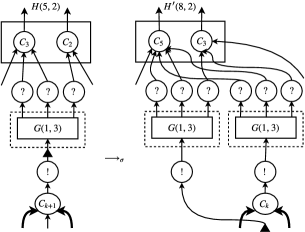
Figure 7. Example of Rewrite Transition $\to_{\sigma}$

All pass and rewrite transitions are well-defined, and indeed deterministic. Pass transitions are also reversible, in the sense that no two different pass transitions result in the same graph state. No transition is possible at a final state, and no pass transition results in an initial state. An execution of pass transitions only has some continuity in the following sense.

Lemma 2 (Pass continuity).

For any execution $\mathit{Init}(G)\to^{*}((G,e),\delta)$ of pass transitions only, there exists a non-empty sequence $e_{1},\ldots,e_{n}$ of links of $G$ that satisfies the following.

• $e_{1}$ is the root of $G$, and $e_{n}=e$.

• For each $i\in\{1,\ldots,n-1\}$, there exists a node whose inputs include $e_{i}$ and whose outputs include $e_{i+1}$.

• Each link in the sequence appears as a token position in the execution $\mathit{Init}(G)\to^{*}((G,e),\delta)$.

Proof 3.1 (Proof outline).

The proof is by induction on the length $k$ of the execution $\mathit{Init}(G)\to^{*}((G,e),\delta)$. In the base case, where $k=0$, the link $e$ is the root of $G$, and $e$ itself as a sequence satisfies the conditions. The inductive case, where $k>0$, is proved by inspecting all possibilities of the last pass transition in the sequence.

The following “sub-graph” property is essential in time-cost analysis, because it bounds the size of duplicable sub-graphs (i.e. $\mathop{!}$-boxes) in an execution.

Lemma 3 (Sub-graph property).

For any execution $\mathit{Init}(G)\to^{*}((H,e),\delta)$, each $\mathop{!}$-box of the graph $H$ appears as a sub-graph of the initial graph $G$.

Proof 3.2.

Rewrite transitions can only copy or discard a $\mathop{!}$-box, and cannot introduce, expand or reduce a single $\mathop{!}$-box. Therefore, any $\mathop{!}$-box of $H$ has to be already a $\mathop{!}$-box of the initial graph $G$.

When a graph has an edge between links, the token is just passed along. With this pass transition over a link at hand, the equivalence relation between graphs that identifies consecutive links with a single link—so-called “wire homeomorphism” [Kis12]—lifts to a weak bisimulation between graph states. Therefore, behaviourally, we can safely ignore consecutive links. From the perspective of time-cost analysis, we benefit from the fact that rewrite transitions are designed not to introduce any edge between links. This means, by assuming that an execution starts with a graph with no consecutive links, we can analyse time cost of the execution without caring the extra pass transition over a link.

4. Implementation of Evaluation Strategies

The implementation of the term calculus, by means of the dynamic GoI, starts with translating (enriched) terms into graphs. The definition of the translation uses multisets of variables, to track how many times each variable occurs in a term. We assume that terms are alpha-converted in a form in which all binders introduce distinct variables. [Multiset] We write $x\in^{k}M$ if the multiplicity of $x$ in a multiset $M$ is $k$. The empty multiset is denoted by $\emptyset$. The sum of two multisets $M_{1}$ and $M_{2}$, denoted by $M_{1}+M_{2}$, is defined as follows: $x\in^{k}{M_{1}+M_{2}}$ if there exist $k_{1}$ and $k_{2}$ such that $x\in^{k_{1}}M_{1}$, $x\in^{k_{2}}M_{2}$ and $k=k_{1}+k_{2}$. Removing all $x$ from a multiset $M$ yields the multiset $M\backslash x$, e.g. ${[x,x,y]\backslash x}=[y]$. We abuse the notation and refer to a multiset $[x,\ldots,x]$ of a finite number of $x$’s, simply as $x$. [Free variables] The map $\mathit{FV}$ of terms to multisets of variables is inductively defined as below, where $\mathbin{\$}\in\{\mathbin{@},\mathbin{\overrightarrow{@}},\mathbin{\overleftarrow{@}}\}$:

$$\mathit{FV}(x) :=[x], \mathit{FV}(\lambda{x}.t) :=\mathit{FV}(t)\backslash x,$$

$$\mathit{FV}(t\mathbin{\$}u) :=\mathit{FV}(t)+\mathit{FV}(u), \mathit{FV}(t[x\leftarrow u]) :=(\mathit{FV}(t)\backslash x)+\mathit{FV}(u).$$

For a multiset $M$ of variables, the map $\mathit{FV}_{M}$ of evaluation contexts to multisets of variables is defined by:

$$\mathit{FV}_{M}(\langle\cdot\rangle) :=M,$$

$$\mathit{FV}_{M}(E\mathbin{@}t) :=\mathit{FV}_{M}(E)+\mathit{FV}(t),$$

$$\mathit{FV}_{M}(E\mathbin{\overrightarrow{@}}t) :=\mathit{FV}_{M}(E)+\mathit{FV}(t),$$

$$\mathit{FV}_{M}(A\langle v\rangle\mathbin{\overrightarrow{@}}E) :=\mathit{FV}(A\langle v\rangle)+\mathit{FV}_{M}(E),$$

$$\mathit{FV}_{M}(t\mathbin{\overleftarrow{@}}E) :=\mathit{FV}(t)+\mathit{FV}_{M}(E),$$

$$\mathit{FV}_{M}(E\mathbin{\overleftarrow{@}}A\langle v\rangle) :=\mathit{FV}_{M}(E)+\mathit{FV}(A\langle v\rangle),$$

$$\mathit{FV}_{M}(E[x\leftarrow t]) :=(\mathit{FV}_{M}(E)\backslash x)+\mathit{FV}(t),$$

$$\mathit{FV}_{M}(E^{\prime}\langle x\rangle[x\leftarrow E]) :=(\mathit{FV}(E^{\prime}\langle x\rangle)\backslash x)+\mathit{FV}_{M}(E).$$

A term $t$ is said be closed if $\mathit{FV}(t)=\emptyset$. Consequences of the above definition are the following equations.

$$\mathit{FV}(E\langle t\rangle) =\mathit{FV}_{\mathit{FV}(t)}(E),$$

$$\mathit{FV}_{M}(E\langle E^{\prime}\rangle) =\mathit{FV}_{\mathit{FV}_{M}(E^{\prime})}(E),$$

$$\mathit{FV}_{M+M^{\prime}}(E) =\mathit{FV}_{M}(E)+M^{\prime}\quad\text{(if $M^{\prime}$ is not captured in $E$)},$$

$$\mathit{FV}_{x}(E)\backslash x =\mathit{FV}_{\emptyset}(E)\backslash x.$$

We give translations of terms, answer contexts, and evaluation contexts separately. Fig. 12 and Fig. 12 define two mutually recursive translations $(\cdot)^{\dagger}$ and $(\cdot)^{\ddagger}$, the first one for terms and answer contexts, and the second one for evaluation contexts. In the figures, ${\mathbin{\$}}\in\{\mathbin{@},\mathbin{\overrightarrow{@}},\mathbin{\overleftarrow{@}}\}$, and $m$ is the multiplicity of $x$. Fig. 9 shows the general form of the translations, and Fig. 9 shows translation of a term $((\lambda{f}.\lambda{x}.f\mathbin{@}(f\mathbin{@}x))\mathbin{@}(\lambda{y}.y))\mathbin{@}(\lambda{z}.z)$.

Figure 8. General Form of Translations

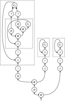
Figure 9. Translation of a Term
$((\lambda{f}.\lambda{x}.f\mathbin{@}(f\mathbin{@}x))\mathbin{@}(\lambda{y}.y))\mathbin{@}(\lambda{z}.z)$

The DGoIM can evaluate a closed term $t$ by starting an execution on the translation $t^{\dagger}$. Executions on any translated closed pure terms can be seen in our on-line visualiser. The translations of answer contexts and evaluation contexts are to define a weak simulation of the sub-machine semantics by the DGoIM, which is then used to prove soundness, completeness and efficiency of the DGoIM.

The annotation of bold-stroke edges means each edge of a bunch is labelled with an element of the annotating multiset, in a one-to-one manner. In particular if a bold-stroke edge is annotated by a variable $x$, all edges in the bunch are annotated by the variable $x$. Translation $E^{\ddagger}_{M}$ of an evaluation context has one input and one output that are not annotated, which we refer to as the “main” input and the “main” output. These annotations are only used to define the translations, and are subsequently ignored during execution.

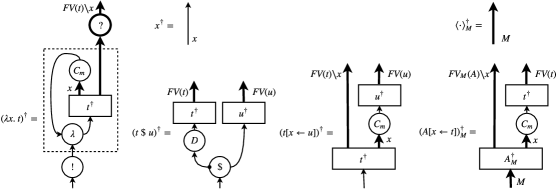
where $\$\in\{\mathbin{@},\mathbin{\overrightarrow{@}},\mathbin{\overleftarrow{@}}\}$.

Figure 10. Inductive Translation of Terms and Answer Contexts

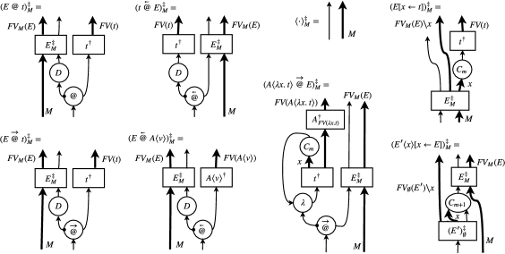
Figure 11. Inductive Translation of Evaluation Contexts

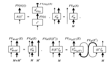
Figure 12. Decompositions of Translations

The translations are based on the so-called “call-by-value” translation of linear logic to intuitionistic logic (e.g. [MOTW99]). Only the translation of abstraction can be accompanied by a $\mathop{!}$-box, which captures the fact that only values (i.e. abstractions) can be duplicated (see the basic rule (10) in Fig. 1). Note that only one $\mathit{C}$-node is introduced for each bound variable. This is vital to achieve constant cost in looking up a variable, namely in realising the basic rule (9) in Fig. 1.

The two mutually recursive translations $(\cdot)^{\dagger}$ and $(\cdot)^{\ddagger}$ are related by the decompositions in Fig. 12, which can be checked by straightforward induction. In the third decomposition, $M^{\prime}$ is not captured in $E$. Note that, in general, the translation $E\langle t\rangle^{\dagger}$ of a term in an evaluation context cannot be decomposed into translations $E^{\ddagger}_{\mathit{FV}(t)}$ and $t^{\dagger}$. This is because a translation $(A\langle\lambda{x}.t\rangle\mathbin{\overrightarrow{@}}E)^{\ddagger}_{M}$ lacks a $\mathop{!}$-box structure, compared to a translation $(A\langle\lambda{x}.t\rangle\mathbin{\overrightarrow{@}}u)^{\dagger}$.

Translation of an evaluation context can be traversed by pass transitions without raising the rewrite flag $\lambda$ or $\mathop{!}$, as the following lemma states.

Lemma 4.

Let $E$ be an evaluation context and $M$ be a multiset. For any graph $G(1,0)$ that has $E^{\ddagger}_{M}$ as a sub-graph and has no edge between links, let $e_{i}$ and $e_{o}$ be the main input and the main output of the sub-graph $E^{\ddagger}_{M}$, respectively. For any pair $(S,B)$ of a computation stack and a box stack, there exists a pair $(S^{\prime},B^{\prime})$ of a computation stack and a box stack, such that $((G,e_{i}),(\mathord{\uparrow},\square,S,B))\to^{*}((G,e_{o}),(\mathord{\uparrow},\square,S^{\prime},B^{\prime}))$ is a sequence of pass transitions.

Proof 4.1.

By induction on $E$. We use $\overset{p}{\to}^{*}$ to denote a sequence of pass transitions in this proof. In the base case, where $E=\langle\cdot\rangle$, the main input $e_{i}$ and the main output $e_{o}$ coincides. An empty sequence suffices.

The first class of inductive cases are when the top-level constructor of $E$ is function application, e.g. $E\equiv E^{\prime}\mathbin{@}t$. Let $e^{\prime}_{i}$ and $e^{\prime}_{o}$ be the main input and the main output of the sub-graph $(E^{\prime})^{\ddagger}_{M}$, respectively. In each of the cases, there exist stacks $S^{\prime\prime}$ and $B^{\prime\prime}$ such that $((G,e_{i}),(\mathord{\uparrow},\square,S,B))\overset{p}{\to}^{*}((G,e^{\prime}_{i}),(\mathord{\uparrow},\square,S^{\prime\prime},B^{\prime\prime}))$. By the induction hypothesis, there exist stacks $S^{\prime}$ and $B^{\prime}$ such that $((G,e^{\prime}_{i}),(\mathord{\uparrow},\square,S^{\prime\prime},B^{\prime\prime}))\overset{p}{\to}^{*}((G,e^{\prime}_{o}),(\mathord{\uparrow},\square,S^{\prime},B^{\prime}))$. Combining these two sequences yields a desired sequence, because $e^{\prime}_{o}=e_{o}$.

The inductive case where $E\equiv E^{\prime}[x\leftarrow t]$ simply boils down to the induction hypothesis.

The last inductive case is when $E\equiv E_{1}\langle x\rangle[x\leftarrow E_{2}]$. Let $e^{\prime}_{i}$ and $e^{\prime}_{o}$ be the main input and the main output of the sub-graph $(E_{1})^{\ddagger}_{\emptyset}$, and $e^{\prime\prime}_{i}$ and $e^{\prime\prime}_{o}$ be the main input and the main output of the sub-graph $(E_{2})^{\ddagger}_{M}$, respectively. We have $e_{i}=e^{\prime}_{i}$ and $e_{o}=e^{\prime\prime}_{o}$. The link $e^{\prime}_{o}$ is an input of a $\mathit{C}$-node and $e^{\prime\prime}_{i}$ is the output of the $\mathit{C}$-node. By the induction hypothesis on $E_{1}$, there exist stacks $S^{\prime\prime}$ and $B^{\prime\prime}$ such that $((G,e^{\prime}_{i}),(\mathord{\uparrow},\square,S,B))\overset{p}{\to}^{*}((G,e^{\prime}_{o}),(\mathord{\uparrow},\square,S^{\prime\prime},B^{\prime\prime}))$. This sequence can be followed by a pass transition $((G,e^{\prime}_{o}),(\mathord{\uparrow},\square,S^{\prime\prime},B^{\prime\prime}))\to((G,e^{\prime\prime}_{i}),(\mathord{\uparrow},\square,S^{\prime\prime},e^{\prime}_{o}:B^{\prime\prime}))$. By the induction hypothesis on $E_{2}$, there exist stacks $S^{\prime}$ and $B^{\prime}$ such that $((G,e^{\prime\prime}_{i}),(\mathord{\uparrow},\square,S^{\prime\prime},e^{\prime}_{o}:B^{\prime\prime}))\overset{p}{\to}^{*}((G,e^{\prime\prime}_{o}),(\mathord{\uparrow},\square,S^{\prime},B^{\prime}))$. Combining all these sequences yields a desired sequence, because $e_{i}=e^{\prime}_{i}$ and $e_{o}=e^{\prime\prime}_{o}$.

The inductive translations lift to a binary relation between closed enriched terms and graph states. [Binary relation $\preceq$] The binary relation $\preceq$ is defined by $E\langle\llparenthesis t\rrparenthesis\rangle\preceq((E^{\ddagger}\circ t^{\dagger},e),(\mathord{\uparrow},\square,S,B))$, where: (i) $E\langle\llparenthesis t\rrparenthesis\rangle$ is a closed enriched term, and $(E^{\ddagger}\circ t^{\dagger},e)$ is given by with no edges between links, and (ii) there is an execution $\mathit{Init}(E^{\ddagger}\circ t^{\dagger})\to^{*}((E^{\ddagger}\circ t^{\dagger},e),(\mathord{\uparrow},\square,S,B))$ of pass transitions only, in which $e$ appears as a token position only in the last state. A special case is $\llparenthesis t\rrparenthesis\preceq\mathit{Init}(t^{\dagger})$, which relates the starting points of an evaluation and an execution. We require the graph $E^{\ddagger}\circ t^{\dagger}$ to have no edges between links, which is based on the discussion at the end of Sec. 3 and essential for time-cost analysis. Although the definition of the translations uses edges between links (e.g. the translation $x^{\dagger}$), the graphs $E^{\ddagger}$ and $t^{\dagger}$ can be constructed without introducing any edge between links. For example, a variable can be translated into a single link that is both an input and an output, and outputs of the translation $(t\mathbin{@}u)^{\dagger}$ can be simply the union of outputs of $t^{\dagger}$ and $u^{\dagger}$. The graph $E^{\ddagger}\circ t^{\dagger}$ can be constructed by identifying interfaces of $E^{\ddagger}$ and $t^{\dagger}$, instead of introducing edges.

The binary relation $\preceq$ gives a weak simulation of the sub-machine semantics by the graph-rewriting machine. The weakness, i.e. the extra transitions compared with reductions, comes from the locality of pass transitions and the bureaucracy of managing $\mathop{!}$-boxes.

Theorem 5 (Weak simulation with global bound).

1. If $E\langle\llparenthesis t\rrparenthesis\rangle\multimap_{\chi}E^{\prime}\langle\llparenthesis t^{\prime}\rrparenthesis\rangle$ and $E\langle\llparenthesis t\rrparenthesis\rangle\preceq((E^{\ddagger}\circ t^{\dagger},e),\delta)$ hold, then there exists a number $n\leq 3$ and a graph state $(((E^{\prime})^{\ddagger}\circ(t^{\prime})^{\dagger},e^{\prime}),\delta^{\prime})$ such that $((E^{\ddagger}\circ t^{\dagger},e),\delta)\to_{\epsilon}^{n}\to_{\chi}(((E^{\prime})^{\ddagger}\circ(t^{\prime})^{\dagger},e^{\prime}),\delta^{\prime})$ and $E^{\prime}\langle\llparenthesis t^{\prime}\rrparenthesis\rangle\preceq(((E^{\prime})^{\ddagger}\circ(t^{\prime})^{\dagger},e^{\prime}),\delta^{\prime})$.

2. If $A\langle\llparenthesis v\rrparenthesis\rangle\preceq((A^{\ddagger}\circ v^{\dagger},e),\delta)$ holds, then the graph state $((A^{\ddagger}\circ v^{\dagger},e),\delta)$ is initial, from which only the transition $\mathit{Init}(A^{\ddagger}\circ v^{\dagger})\to_{\epsilon}\mathit{Final}(A^{\ddagger}\circ v^{\dagger})$ is possible.

Proof 4.2.

For the second half, $e$ is the root of the graph $A^{\ddagger}\circ v^{\dagger}$, which means the state $((A^{\ddagger}\circ v^{\dagger},e),\delta)$ is not a result of any pass transition. Therefore, by the condition (ii) of the binary relation $\preceq$, we have $\mathit{Init}(A^{\ddagger}\circ v^{\dagger})=((A^{\ddagger}\circ v^{\dagger},e),\delta)$, and one pass transition from this state yields a final state $\mathit{Final}(A^{\ddagger}\circ v^{\dagger})$.

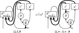
(4)  $E\langle A\langle\llparenthesis\lambda{x}.t\rrparenthesis\rangle\mathbin{\overrightarrow{@}}u\rangle\multimap_{\epsilon}E\langle A\langle\lambda{x}.t\rangle\mathbin{\overrightarrow{@}}\llparenthesis u\rrparenthesis\rangle$

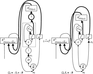
(5)  $E\langle A\langle\lambda{x}.t\rangle\mathbin{\overrightarrow{@}}A^{\prime}\langle\llparenthesis v\rrparenthesis\rangle\rangle\multimap_{\beta}E\langle A\langle\llparenthesis t\rrparenthesis[x\leftarrow A^{\prime}\langle v\rangle]\rangle\rangle$

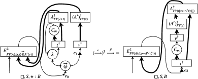
Figure 13. Illustration of Simulation: Left-to-Right Call-by-Value Application

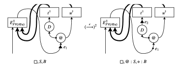
(2)  $E\langle A\langle\llparenthesis\lambda{x}.t\rrparenthesis\rangle\mathbin{@}u\rangle\multimap_{\beta}E\langle A\langle\llparenthesis t\rrparenthesis[x\leftarrow u]\rangle\rangle$

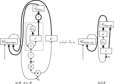
(9)  $E\langle E^{\prime}\langle\llparenthesis x\rrparenthesis\rangle[x\leftarrow A\langle u\rangle]\rangle\multimap_{\epsilon}E\langle E^{\prime}\langle x\rangle[x\leftarrow A\langle\llparenthesis u\rrparenthesis\rangle]\rangle$

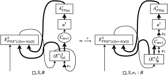
(10)  $E\langle E^{\prime}\langle x\rangle[x\leftarrow A\langle\llparenthesis v\rrparenthesis\rangle]\rangle\multimap_{\sigma}E\langle A\langle E^{\prime}\langle\llparenthesis v\rrparenthesis\rangle[x\leftarrow v]\rangle\rangle$

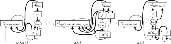
Figure 14. Illustration of Simulation: Call-by-Need Application and Explicit Substitutions

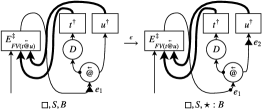
(7)  $E\langle t\mathbin{\overleftarrow{@}}A\langle\llparenthesis v\rrparenthesis\rangle\rangle\multimap_{\epsilon}E\langle\llparenthesis t\rrparenthesis\mathbin{\overleftarrow{@}}A\langle v\rangle\rangle$

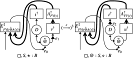
(8)  $E\langle A\langle\llparenthesis\lambda{x}.t\rrparenthesis\rangle\mathbin{\overleftarrow{@}}A^{\prime}\langle v\rangle\rangle\multimap_{\beta}E\langle A\langle\llparenthesis t\rrparenthesis[x\leftarrow A^{\prime}\langle v\rangle]\rangle\rangle$

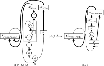
Figure 15. Illustration of Simulation: Right-to-Left Call-by-Value Application

For the first half, Fig. 13, Fig. 14 and Fig. 15 illustrate how the graph-rewriting machine simulates each reduction $\multimap$ of the sub-machine semantics. Each sequence of transitions $\to$ simulates a single reduction $\multimap$. Annotations of edges are omitted, and only the first and the last states of each sequence are shown, except for the case of the basic rule (10).

Some sequences involve equations that apply the four decomposition properties of the translations $(\cdot)^{\dagger}$ and $(\cdot)^{\ddagger}$, which are given earlier in this section. These equations rely on the fact that terms are alpha-converted in a form in which all binders introduce distinct variables, and reductions with labels $\beta$ and $\sigma$ work modulo alpha-equivalence to avoid name captures. This implies the following.

• Free variables of $u$ are not captured by $A$ in the case of the basic rule (2).

• Free variables of $A^{\prime}\langle v\rangle$ are not captured by $A$ in the case of the basic rules (5) and (8).

• The variable $x$ is not captured by $E$ or $E^{\prime}$ in the case of the basic rules (9) and (10).

• In the case of the basic rule (10), free variables of $E^{\prime}$ are not captured by $A$, free variables of $v$ are not captured by $E^{\prime}$, and $x$ does not freely appear in $v$.

Simulation of the basic rule (10) involves duplicating the sub-graph $v^{\dagger}$, which is a $\mathop{!}$-box. Because free variables of the value $v$ are captured by either $E$ or $A$, the multiset $\mathit{FV}(v)$ can be partitioned into two multisets as $\mathit{FV}(v)=M_{E}+M_{A}$, such that $M_{E}$ is the multiset of those captured by $E$ and $M_{A}$ is the multiset of those captured by $A$. No variable is contained by both $M_{E}$ and $M_{A}$. The translations $E^{\ddagger}$ and $A^{\dagger}$ include $\mathit{C}$-nodes that correspond to $M_{E}$ and $M_{A}$, respectively. These $\mathit{C}$-nodes get extra inputs by the rewrite transition labelled with $\sigma$, as represented by the middle state in the simulation sequence.

In each sequence, let $G_{s}$ and $G_{t}$ be the first and the last graph, respectively. By the condition (ii) of the binary relation $\preceq$, there exists an execution $\mathit{Exec}:\mathit{Init}(G_{s})\to^{*}((G_{s},e_{1}),(\mathord{\uparrow},\square,S^{\prime},B^{\prime}))$ of only pass transitions, in which the link $e_{1}$ (see the figures) appears as a token position only once at the end.

1. In simulation of the basic rules (1), (3) and (6), the figures use $S$ and $B$ instead of $S^{\prime}$ and $B^{\prime}$. By Lem. 2, the result position $e_{2}$ (see the figures) does not appear in the execution $\mathit{Exec}$; if this is not the case, $e_{1}$ would appear more than once in $\mathit{Exec}$, which is a contradiction. Therefore, $\mathit{Exec}$ followed by the pass transitions shown in the figures gives a desired execution that meets the condition (ii) of the binary relation $\preceq$.

2. In simulation of the basic rule (9), the figure uses $S$ and $B$ instead of $S^{\prime}$ and $B^{\prime}$. Because $x$ is not captured by $E^{\prime}$, the starting position $e_{1}$ is in fact an input of the $\mathit{C}_{m+1}$-node. Using Lem. 2 again in the same way, the result position $e_{2}$ does not appear in the execution $\mathit{Exec}$. Therefore, $\mathit{Exec}$ followed by the pass transition shown in the figures gives a desired execution that meets the condition (ii) of the binary relation $\preceq$.

3. In simulation of the basic rule (7), by the reversibility of pass transitions, there exist stacks $S$ and $B$ such that: $S^{\prime}=S$, $B^{\prime}=\star:B$, and the execution $\mathit{Exec}$ can be decomposed into an execution $\mathit{Exec}^{\prime}:\mathit{Init}(G_{s})\to^{*}((G_{s},e_{0}),(\mathord{\uparrow},\square,S,B))$ and one subsequent pass transition (see the figure for $e_{0}$). In the execution $\mathit{Exec}^{\prime}$, the link $e_{0}$ appears as a token position only once at the end, which can be checked by contradiction as follows.

   • If $e_{0}$ appears more than once in $\mathit{Exec}^{\prime}$ and its first appearance is with direction $\mathord{\downarrow}$, it must be a result of a pass transition. However, no pass transition leads to this situation, because $e_{0}$ is an input of a function application node. This is a contradiction.

   • If $e_{0}$ appears more than once in $\mathit{Exec}^{\prime}$ and its first appearance is with direction $\mathord{\uparrow}$, it must be with rewrite flag $\square$, because $\mathit{Exec}^{\prime}$ consists of pass transitions only. Regardless of token data, the first appearance leads to an extra appearance of $e_{1}$ in $\mathit{Exec}^{\prime}$, which is a contradiction.

   Given this freshness of $e_{0}$ in $\mathit{Exec}^{\prime}$, by Lem. 2, the result position $e_{2}$ does not appear in the execution $\mathit{Exec}^{\prime}$. Therefore, $\mathit{Exec}$ followed by the pass transitions shown in the figures gives a desired execution that meets the condition (ii) of the binary relation $\preceq$.

4. In simulation of the basic rules (2), (5) and (8), by the reversibility of pass transitions, there exist stacks $S$ and $B$ such thatthe execution $\mathit{Exec}$ can be decomposed into an execution $\mathit{Exec}^{\prime}:\mathit{Init}(G_{s})\to^{*}((G_{s},e_{0}),(\mathord{\uparrow},\square,S,B))$ and at least one subsequent pass transition. In the execution $\mathit{Exec}^{\prime}$, the link $e_{0}$ appears as a token position only once at the end, which can be checked in the same manner as the previous case (3). Using this freshness of $e_{0}$ in $\mathit{Exec}^{\prime}$ and Lem. 2, we can conclude that any node that interacts with a token in the execution $\mathit{Exec}^{\prime}$ (i.e. that is relevant in a pass transition in the execution $\mathit{Exec}^{\prime}$) belongs to $E^{\ddagger}$. This means that any pass transition in $\mathit{Exec}^{\prime}$, on the starting graph $G_{s}$, can be imitated in the resulting graph $G_{t}$. Namely, the link $e_{0}$ corresponds to the result position $e_{2}$, and $\mathit{Exec}^{\prime}$ corresponds to an execution $\mathit{Exec}^{\prime\prime}:\mathit{Init}(G_{t})\to^{*}((G_{t},e_{2}),(\mathord{\uparrow},\square,S,B))$ of only pass transitions, in which $e_{2}$ appears only once at the end. This execution $\mathit{Exec}^{\prime\prime}$ gives a desired execution that meets the condition (ii) of the binary relation $\preceq$.

5. In simulation of the basic rule (4), the same reasoning as the previous case (4) gives an execution $\mathit{Exec}^{\prime\prime}:\mathit{Init}(G_{t})\to^{*}((G_{t},e_{0}),(\mathord{\uparrow},\square,S,B))$ of only pass transitions, in which $e_{0}$ appears only once at the end. By Lem. 2, the result position $e_{2}$ does not appear in the execution $\mathit{Exec}^{\prime\prime}$. Therefore, $\mathit{Exec}^{\prime\prime}$ followed by pass transitions gives a desired execution that meets the condition (ii) of the binary relation $\preceq$.

6. In simulation of the basic rule (10), by the reversibility of pass transitions, there exist an input $e_{0}$ of the $\mathit{C}_{m+1}$-node and stacks $S$ and $B$ such that: $S^{\prime}=S$, $B^{\prime}=e_{0}:B$, and the execution $\mathit{Exec}$ can be decomposed into an execution $\mathit{Exec}^{\prime}:\mathit{Init}(G_{s})\to^{*}((G_{s},e_{0}),(\mathord{\uparrow},\square,S,B))$ and one subsequent pass transition that pushes $e_{0}$ to the box stack. By Lem. 2, the link $e_{3}$ (see the figure) appears in the execution $\mathit{Exec}^{\prime}$. Analysing this appearance, we can conclude that the link $e_{0}$ is in fact the main output of $(E^{\prime})^{\ddagger}_{\emptyset}$.

   • If $e_{3}$ appears with direction $\mathord{\downarrow}$ in $\mathit{Exec}^{\prime}$, because $e_{3}$ is an input of a function application node or a $\mathit{C}$-node, this appearance cannot be a result of any pass transition. This is a contradiction.

   • If $e_{3}$ appears with direction $\mathord{\uparrow}$, it must be with rewrite flag $\square$, because $\mathit{Exec}^{\prime}$ consists of pass transitions only. Because $e_{3}$ is the main input of $(E^{\prime})^{\ddagger}_{\emptyset}$, by Lem. 4, this appearance leads to a state whose token position is the main output $e^{\prime}$ of $(E^{\prime})^{\ddagger}_{\emptyset}$, direction is $\mathord{\uparrow}$ and rewrite flag is $\square$. One pass transition from the state leads to a state whose token position is $e_{1}$. This means there exists an execution $\mathit{Exec}^{\prime\prime\prime}$ of pass transitions only, via the token position $e_{3}$ and the second last token position $e^{\prime}$, to the token position $e_{1}$. Because pass transitions are deterministic, it is either: (1) $\mathit{Exec}$ is strictly a sub-sequence of $\mathit{Exec}^{\prime\prime\prime}$, (2) $\mathit{Exec}=\mathit{Exec}^{\prime\prime\prime}$, or (3) $\mathit{Exec}^{\prime\prime\prime}$ is strictly a sub-sequence of $\mathit{Exec}$. Because $\mathit{Exec}$ is followed by a pass transition and a rewrite transition as shown in the figure, the case (1) is impossible. Because $e_{1}$ appears only once at the end in the execution $\mathit{Exec}$, the case (3) leads to a contradiction. Therefore we can conclude that (2) is the case, i.e. $\mathit{Exec}=\mathit{Exec}^{\prime\prime\prime}$. This means $e^{\prime}=e_{0}$, i.e. $e_{0}$ is the main output of $(E^{\prime})^{\ddagger}_{\emptyset}$.

   As a consequence, the link $e_{2}$ is indeed the result position, corresponding to the link $e_{0}$.

   The rest of the reasoning is similar to the case 4. In the execution $\mathit{Exec}$ to the starting position $e_{1}$, the token does not interact with nodes that belong to $A^{\dagger}$ or $v^{\dagger}$; otherwise, by Lem. 2, $e_{1}$ would have an extra appearance in $\mathit{Exec}$, which is a contradiction. For the same reason, the execution $\mathit{Exec}^{\prime}$ to the link $e_{0}$ does not involve any interaction of the token with the $\mathit{C}_{m+1}$-node, and hence $e_{0}$ appears only once at the end in the execution $\mathit{Exec}^{\prime}$. As a result, the execution $\mathit{Exec}^{\prime}$ gives an execution $\mathit{Exec}^{\prime\prime}:\mathit{Init}(G_{t})\to^{*}((G_{t},e_{2}),(\mathord{\uparrow},\square,S,B))$ of only pass transitions on the resulting graph $G_{t}$, in which $e_{2}$ appears only once at the end. This execution $\mathit{Exec}^{\prime\prime}$ gives a desired execution that meets the condition (ii) of the binary relation $\preceq$.

(3)  $E\langle\llparenthesis t\mathbin{\overrightarrow{@}}u\rrparenthesis\rangle\multimap_{\epsilon}E\langle\llparenthesis t\rrparenthesis\mathbin{\overrightarrow{@}}u\rangle$

(1)  $E\langle\llparenthesis t\mathbin{@}u\rrparenthesis\rangle\multimap_{\epsilon}E\langle\llparenthesis t\rrparenthesis\mathbin{@}u\rangle$

(6)  $E\langle\llparenthesis t\mathbin{\overleftarrow{@}}u\rrparenthesis\rangle\multimap_{\epsilon}E\langle t\mathbin{\overleftarrow{@}}\llparenthesis u\rrparenthesis\rangle$

5. Time-Cost Analysis

We analyse how time-efficiently the token-guided graph-rewriting machine implements evaluation strategies, following the methodology developed by Accattoli et al. [ABM14, AS14, Acc17]. The time-cost analysis focuses on how efficiently an abstract machine implements an evaluation strategy. In other words, we are not interested in minimising the number of $\beta$-reduction steps simulated by an abstract machine. Our aim is to see if the number of transitions of an abstract machine is “reasonable”, compared to the number of necessary $\beta$-reduction steps determined by a given evaluation strategy.

Accattoli’s methodology assumes that an abstract machine has three groups of transitions: 1) “$\beta$-transitions” that correspond to $\beta$-reduction in which substitution is delayed, 2) transitions that perform substitution, and 3) other “overhead” transitions. We incorporate this classification using the labels $\beta$, $\sigma$ and $\epsilon$ of transitions.

Another assumption of the methodology is that, each step of $\beta$-reduction is simulated by a single transition of an abstract machine, and so is substitution of each occurrence of a variable. This is satisfied by many known abstract machines, including Danvy and Zerny’s storeless abstract machine [DZ13] that our sub-machine semantics resembles, however not by the token-guided graph-rewriting abstract machine. The machine has “finer” transitions and can take several transitions to simulate a single step of reduction, as we can observe in Thm. 5. In spite of this mismatch we can still follow the methodology, thanks to the weak simulation $\preceq$. It discloses what transitions of the token-guided graph-rewriting machine exactly correspond to $\beta$-reduction and substitution, and gives a concrete number of overhead transitions that the machine needs to simulate $\beta$-reduction and substitution.

The methodology of time-cost analysis has four steps: (I) bound the number of transitions required in implementing evaluation strategies, (II) estimate time cost of each transition, (III) bound overall time cost of implementing evaluation strategies, by multiplying the number of transitions with time cost for each transition, and finally (IV) classify the abstract machine according to its execution time cost. Consider now the following taxonomy of abstract machines introduced in [Acc17]. [classes of abstract machines [Acc17, Def. 7.1]]

1. An abstract machine is efficient if its execution time cost is linear in both the input size and the number of $\beta$-transitions.

2. An abstract machine is reasonable if its execution time cost is polynomial in the input size and the number of $\beta$-transitions.

3. An abstract machine is unreasonable if it is not reasonable.

In our case, the input size is given by the size $|t|$ of the term $t$, inductively defined by:

$$|x| :=1, |\lambda{x}.t| :=|t|+1,$$

$$|t\mathbin{@}u|=|t\mathbin{\overrightarrow{@}}u|=|t\mathbin{\overleftarrow{@}}u| :=|t|+|u|+1, |t[x\leftarrow u]| :=|t|+|u|+1.$$

The number of $\beta$-transitions is simply the number of transitions labelled with $\beta$, which in fact corresponds to the number of reductions labelled with $\beta$, thanks to Thm. 5.

Given an evaluation $\mathit{Eval}$, the number of occurrences of a label $\chi$ is denoted by $|\mathit{Eval}|_{\chi}$. The sub-machine semantics comes with the following quantitative bounds.

Proposition 6.

For any pure closed term $t$ and any evaluation $\mathit{Eval}\colon\llparenthesis t\rrparenthesis\multimap^{*}A\langle\llparenthesis v\rrparenthesis\rangle$ that terminates, the number of reductions is bounded by $|\mathit{Eval}|_{\sigma}=\mathcal{O}(|\mathit{Eval}|_{\beta})$ and $|\mathit{Eval}|_{\epsilon}=\mathcal{O}(|t|\cdot|\mathit{Eval}|_{\beta}).$

Proof 5.1.

A term uses a single evaluation strategy, either call-by-need, left-to-right call-by-value, or right-to-left call-by-value. Forgetting the window of an enriched term $E\langle\llparenthesis t\rrparenthesis\rangle$ gives a term $E\langle t\rangle$, which can be seen as a term of the linear substitution calculus [AK10]. This gives an one-to-one correspondence between an evaluation by the sub-machine semantics and a “derivation” in the linear substitution calculus, via the concept of “distillery” [ABM14, Sec. 4]. The correspondence is in such a way that it enables us to directly apply the bounds about the linear substitution calculus [AS14, Cor. 1 & Thm. 2] and obtain the first equation.

The second equation is proved by combining the first equation and an equation $|\mathit{Eval}|_{\epsilon}=\mathcal{O}(|t|\cdot(|\mathit{Eval}|_{\beta}+|\mathit{Eval}|_{\sigma}))$. This auxiliary equation can be proved using ideas from Accattoli et al.’s analysis of various abstract machines [ABM14, Thm. 11.3 & Thm. 11.5], as below.

For any enriched term $E^{\prime}\langle\llparenthesis t^{\prime}\rrparenthesis\rangle$ that appears in the evaluation $\mathit{Eval}\colon\llparenthesis t\rrparenthesis\multimap^{*}A\langle\llparenthesis v\rrparenthesis\rangle$, we define two measures. The first measure $\#_{1}(E^{\prime}\langle\llparenthesis t^{\prime}\rrparenthesis\rangle)$ is defined by: $|t^{\prime}|+|u|$ if $E^{\prime}$ is in the form of $E^{\prime\prime}\langle A^{\prime}\langle\cdot\rangle\mathbin{@}u\rangle$, $E^{\prime\prime}\langle A^{\prime}\langle\cdot\rangle\mathbin{\overrightarrow{@}}u\rangle$, or $E^{\prime\prime}\langle u\mathbin{\overleftarrow{@}}A^{\prime}\langle\cdot\rangle\rangle$; and $|t^{\prime}|$ otherwise. By Lem. 1, both $t^{\prime}$ and $u$ above are sub-terms of $t$, and we have $\#_{1}(E^{\prime}\langle\llparenthesis t^{\prime}\rrparenthesis\rangle)\leq 2\cdot|t|$. The second measure $\#_{2}(E^{\prime})$ is on $E^{\prime}$ only, and defined inductively as below.

$$\#_{2}(\langle\cdot\rangle):=0,\quad\#_{2}(E^{\prime\prime}\langle x\rangle[x\leftarrow E^{\prime\prime\prime}]) :=\#_{2}(E^{\prime\prime})+\#_{2}(E^{\prime\prime\prime})+1,$$

$$\#_{2}(E^{\prime\prime}\mathbin{@}t)=\#_{2}(E^{\prime\prime}\mathbin{\overrightarrow{@}}t)=\#_{2}(A\langle v\rangle\mathbin{\overrightarrow{@}}E^{\prime\prime}) :=\#_{2}(E^{\prime\prime}),$$

$$\#_{2}(t\mathbin{\overleftarrow{@}}E^{\prime\prime})=\#_{2}(E^{\prime\prime}\mathbin{\overleftarrow{@}}A\langle v\rangle)=\#_{2}(E^{\prime\prime}[x\leftarrow t^{\prime\prime}]) :=\#_{2}(E^{\prime\prime}).$$

Because the basic rules (1), (3), (4), (6) and (7) strictly reduce the measure $\#_{1}$, these rules can be consecutively applied at most $2\cdot|t|$ times. The evaluation $\mathit{Eval}$ can be seen as applications of these rules interleaved with other rules, so the total number of applications of these five basic rules can be bounded by $\mathcal{O}(|t|\cdot(|\mathit{Eval}|_{\beta}+|\mathit{Eval}|_{\sigma}+|\mathit{Eval}|_{9}))$, where $|\mathit{Eval}|_{9}$ denotes the total number of applications of the basic rule (9).

The measure $\#_{2}$ is increased only by the basic rule (9) and decreased only by the basic rule (10). Both the increase and the decrease are of one. Because the measure $\#_{2}$ gives zero for both $\llparenthesis t\rrparenthesis$ and $A\langle\llparenthesis v\rrparenthesis\rangle$, namely $\#_{2}(\langle\cdot\rangle)=\#_{2}(A)=0$, the basic rule (9) must be applied as many times as the basic rule (10) in the evaluation $\mathit{Eval}$. This means $|\mathit{Eval}|_{\sigma}=|\mathit{Eval}|_{9}$.

Combining the bound $\mathcal{O}(|t|\cdot(|\mathit{Eval}|_{\beta}+|\mathit{Eval}|_{\sigma}+|\mathit{Eval}|_{9}))$ with the equation $|\mathit{Eval}|_{\sigma}=|\mathit{Eval}|_{9}$ gives the auxiliary equation on $|\mathit{Eval}|_{\epsilon}$.

We use the same notation $|\mathit{Exec}|_{\chi}$, as for an evaluation, to denote the number of occurrences of each label $\chi$ in an execution $\mathit{Exec}$. Additionally the number of rewrite transitions with the label $\epsilon$, i.e. those that eliminates a $\mathop{!}$-box structure, is denoted by $|\mathit{Exec}|_{\mathit{\epsilon R}}$. Note that pass transitions are all labelled with $\epsilon$, and hence $|\mathit{Exec}|_{\mathit{\epsilon R}}\leq|\mathit{Exec}|_{\epsilon}$. The following proposition completes the first step of the cost analysis.

Proposition 7 (Soundness & completeness, with number bounds).

For any pure closed term $t$, an evaluation $\mathit{Eval}\colon\llparenthesis t\rrparenthesis\multimap^{*}A\langle\llparenthesis v\rrparenthesis\rangle$ terminates with the enriched term $A\langle\llparenthesis v\rrparenthesis\rangle$ if and only if an execution $\mathit{Exec}\colon\mathit{Init}(t^{\dagger})\to^{*}\mathit{Final}(A^{\ddagger}\circ v^{\dagger})$ terminates with the graph $A^{\ddagger}\circ v^{\dagger}$. Moreover the number of transitions is bounded by $|\mathit{Exec}|_{\beta}=|\mathit{Eval}|_{\beta}$, $|\mathit{Exec}|_{\sigma}=\mathcal{O}(|\mathit{Eval}|_{\beta})$, $|\mathit{Exec}|_{\epsilon}=\mathcal{O}(|t|\cdot|\mathit{Eval}|_{\beta})$, $|\mathit{Exec}|_{\mathit{\epsilon R}}=\mathcal{O}(|\mathit{Eval}|_{\beta})$.

Proof 5.2.

Because the initial term $t$ is closed, any enriched term $E^{\prime}\langle\llparenthesis t^{\prime}\rrparenthesis\rangle$ that appears in the evaluation $\mathit{Eval}$ is also closed. This implies that a reduction is always possible at $E^{\prime}\langle\llparenthesis t^{\prime}\rrparenthesis\rangle$ unless it is in the form of $A^{\prime}\langle v^{\prime}\rangle$. In particular, if $t^{\prime}$ is a variable, the variable is captured by an explicit substitution in $E^{\prime}$ and the basic rule (10) is possible. Consequently, if an evaluation of the pure closed term $t$ terminates, the last enriched term is in the form of $A^{\prime}\langle v^{\prime}\rangle$.

The forward direction of the equivalence, that is, the evaluation $\mathit{Eval}$ implies the execution $\mathit{Exec}$, follows from Thm. 5. The backward direction, that is, the execution $\mathit{Exec}$ implies the evaluation $\mathit{Eval}$, also follows from Thm. 5, because an evaluation of the pure closed term $t$ is in the form of $\llparenthesis t\rrparenthesis\multimap^{*}A\langle\llparenthesis v\rrparenthesis\rangle$ or never terminates.

Thm. 5 also gives equations $|\mathit{Exec}|_{\beta}=|\mathit{Eval}|_{\beta}$, $|\mathit{Exec}|_{\sigma}=|\mathit{Eval}|_{\sigma}$ and $|\mathit{Exec}|_{\epsilon}=\mathcal{O}(|\mathit{Eval}|_{\beta}+|\mathit{Eval}|_{\sigma}+|\mathit{Eval}|_{\epsilon})$. Combining these with Prop. 6 yields the desired equations except for the last one (i.e. $|\mathit{Exec}|_{\mathit{\epsilon R}}=\mathcal{O}(|\mathit{Eval}|_{\beta})$).

This last equation follows from an equation $|\mathit{Exec}|_{\mathit{\epsilon R}}=|\mathit{Exec}|_{\beta}$ that can be proved as follows. For any graph state $((G,e),\delta)$ that appears in the execution $\mathit{Exec}\colon\mathit{Init}(t^{\dagger})\to^{*}\mathit{Final}(A^{\ddagger}\circ v^{\dagger})$, we define a measure $\#(G)$ by the number of $\lambda$-nodes that are outside any $\mathop{!}$-box in the graph $G$.

Firstly, at any point of the execution $\mathit{Exec}$, the token is inside a $\mathop{!}$-box if and only if it has the rewrite flag ‘$\mathop{!}$’. This means, if a $\lambda$-node gets eliminated by a rewrite transition labelled with $\beta$, the $\lambda$-node is outside a $\mathop{!}$-box. By Lem. 3, each $\mathop{!}$-box has exactly one $\lambda$-node that directly belongs to it. It follows that each rewrite transition labelled with $\epsilon$ brings exactly one $\lambda$-node outside a $\mathop{!}$-box.

As a result, each rewrite transition labelled with $\beta$ decreases the measure $\#$ by one, and each rewrite transition labelled with $\epsilon$ increases the measure $\#$ by one. No other transitions change the measure $\#$. Because the measure $\#$ gives zero for the initial and final graph states $\mathit{Init}(t^{\dagger})$ and $\mathit{Final}(A^{\ddagger}\circ v^{\dagger})$, namely $\#(t^{\dagger})=\#(A^{\ddagger}\circ v^{\dagger})=0$, we have $|\mathit{Exec}|_{\mathit{\epsilon R}}=|\mathit{Exec}|_{\beta}$.

The next step in the cost analysis is to estimate the time cost of each transition. We assume that graphs are implemented in the following way. Each $\wn$-node, and its input and output, are identified and implemented as a single link. Each link is given by two pointers to its child and its parent. If a node is not a $\wn$-node, it is given by its label, pointers to its inputs, and pointers to its outputs; the pointers to inputs are omitted for $\mathit{C}$-nodes. Additionally, each link and node has a pointer to a $\mathop{!}$-node, or a null pointer, to indicate the $\mathop{!}$-box structure it directly belongs in. Note that each link has at most three pointers, and each node has at most two input (resp. output) pointers, which are distinguished. The size of a graph can be estimated using the number of nodes that are not $\wn$-nodes. Accordingly, a position of the token is a pointer to a link, a direction and a rewrite flag are two symbols, a computation stack is a stack of symbols, and finally a box stack is a stack of symbols and pointers to links.

Using these assumptions of implementation, we estimate time cost of each transition. All pass transitions have constant cost. Each pass transition looks up one node and its outputs (that are either one or two) next to the current position, and involves a fixed number of elements of the token data. Rewrite transitions with the label $\beta$ have constant cost, as they change a constant number of nodes and links, and only a rewrite flag of the token data. Rewrite transitions with the label $\epsilon$ remove a $\mathop{!}$-box structure. This can be done by traversing nodes from its principal door, and hence have cost bounded by the size of the $\mathop{!}$-box. Finally, rewrite transitions with the label $\sigma$ copy a $\mathop{!}$-box structure. Copying cost is bounded by the size of the $\mathop{!}$-box. Updating cost of the sub-graph $H^{\prime}$ (see Fig. 6) is bounded by the number of auxiliary doors, which is less than the size of the copied $\mathop{!}$-box. Updating cost of the $\mathit{C}$-node is constant, because $\mathit{C}$-nodes do not have pointers to its inputs, by the assumption about the implementation of graphs.

With the results of the previous two steps, we can now give the overall time cost of executions and classify our abstract machine.

Theorem 8 (Soundness & completeness, with cost bounds).

For any pure closed term $t$, an evaluation $\mathit{Eval}\colon\llparenthesis t\rrparenthesis\multimap^{*}A\langle\llparenthesis v\rrparenthesis\rangle$ terminates with the enriched term $A\langle\llparenthesis v\rrparenthesis\rangle$ if and only if an execution $\mathit{Exec}\colon\mathit{Init}(t^{\dagger})\to^{*}\mathit{Final}(A^{\ddagger}\circ v^{\dagger})$ terminates with the graph $A^{\ddagger}\circ v^{\dagger}$. The overall time cost of the execution $\mathit{Exec}$ is bounded by $\mathcal{O}(|t|\cdot|\mathit{Eval}|_{\beta})$.

Proof 5.3.

Non-constant cost of rewrite transitions is the size of a $\mathop{!}$-box. By Lem. 3, this size is less than the size of the initial graph $t^{\dagger}$, which can be bounded by the size $|t|$ of the initial term. Therefore any non-constant cost of each rewrite transition, in the execution $\mathit{Exec}$, can be also bounded by $|t|$. By Prop. 7, the overall time cost of rewrite transitions labelled with $\beta$ is $\mathcal{O}(|\mathit{Eval}|_{\beta})$, and that of the other rewrite transitions and pass transitions is $\mathcal{O}(|t|\cdot|\mathit{Eval}|_{\beta})$.

Note that the time cost of constructing the initial graph $t^{\dagger}$, and attaching a token to it, does not affect the bound $\mathcal{O}(|t|\cdot|\mathit{Eval}|_{\beta})$, because it can be done in linear time with respect to $|t|$. This is thanks to the assumption about implementation, namely that $\wn$-nodes and input pointers of $\mathit{C}$-nodes are omitted.

Corollary 9.

The token-guided graph-rewriting machine is an efficient abstract machine implementing call-by-need, left-to-right call-by-value and right-to-left call-by-value evaluation strategies, in the sense of Def. 5.

Cor. 9 classifies the graph-rewriting machine as not just “reasonable”, but in fact “efficient”. In terms of token passing, this efficiency benefits from the graphical representation of environments (i.e. explicit substitutions in our setting). The graphical representation is in such a way that each bound variable is associated with exactly one $\mathit{C}$-node, which is ensured by the translations $(\cdot)^{\dagger}$ and $(\cdot)^{\ddagger}$ and the rewrite transition $\to_{\sigma}$. Excluding any two sequentially-connected $\mathit{C}$-nodes is essential to achieve the “efficient” classification, because it yields the constant cost to look up a bound variable and its associated computation.

As for graph rewriting, the “efficient” classification shows that introduction of graph rewriting to token passing does not bring in any inefficiencies. In our setting, graph rewriting brings in two kinds of non-constant cost. One is duplication cost of a sub-graph, which is indicated by a $\mathop{!}$-box, and the other is elimination cost of a $\mathop{!}$-box that delimits abstraction. Unlike the duplication cost, the elimination cost leads to non-trivial cost that abstract machines in the literature usually do not have. Namely, our graph-rewriting machine simulates a $\beta$-reduction step, in which an abstraction constructor is eliminated and substitution is delayed, at the non-constant cost depending on the size of the abstraction. The time-cost analysis confirms that the duplication cost and the unusual elimination cost have the same impact, on the overall time cost, as the cost of token passing. What is vital here is the sub-graph property (Lem. 3), which ensures that the cost of each duplication and elimination of a $\mathop{!}$-box is always linear in the input size.

6. Rewriting vs. Jumping

The starting point of our development is the GoI-style token-passing abstract machines for call-by-name evaluation, given by Danos and Regnier [DR96], and by Mackie [Mac95]. Fig. 16 recalls these token-passing machines as a version of the DGoIM with the passes-only interleaving strategy (i.e. the DGoIM with only pass transitions). It follows the convention of Fig. 5, but a black triangle in the figure points along (resp. against) the direction of the edge if the token direction is $\mathord{\uparrow}$ (resp. $\mathord{\downarrow}$). Note that this version uses different token data, to which we will come back later.

Token data $(d,S,B,E)$ consists of:

• a direction defined by $d::=\mathord{\uparrow}\mid\mathord{\downarrow}$,

• a computation stack defined by $S::=\square\mid\mathsf{A}:S\mid@:S$, and

• a box stack $B$ and an environment stack $E$, both defined by $B,E::=\square\mid\sigma:B$, using exponential signatures $\sigma::=\star\mid e\cdot\sigma\mid\langle\sigma,\sigma\rangle$ where $e$ is any link of the underlying graph.

Pass transitions:

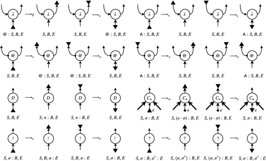
Given a term $t$ with the call-by-need function application ($@$) abused, a successful execution $((t^{\dagger},e_{t}),(\mathord{\uparrow},\square,\square,\square,\square))\to^{*}((t^{\dagger},e_{v}),(\mathord{\uparrow},\square,\square,\square,\square))$ starts at the root $e_{t}$ of the translation $t^{\dagger}$, and ends at the root $e_{v}$ of the translation $v^{\dagger}$, for some sub-value $v$ of the term $t$. The value $v$ indicates the evaluation result.

Figure 16. Passes-Only DGoIM for Call-by-Name [DR96, Mac95]

Token-passing GoI keeps the underlying graph fixed, and re-evaluates a term by repeating token moves. It therefore favours space efficiency at the cost of time efficiency. Repeating token actions poses a challenge for evaluations in which duplicated computation must not lead to repeated evaluation, especially call-by-value evaluation [FM02, Sch14a, HMH14, DFVY15]. Moreover, in call-by-value repeating token actions raises the additional technical challenge of avoiding repeating any associated computational effects [Sch11, MHH16, DFVY17]. A partial solution to this conundrum is to focus on the soundness of the equational theory, while deliberately ignoring the time costs [MHH16]. Introduction of graph reduction, the key idea of the DGoIM, is one total solution in the sense that it avoids repeated token moves and also improves time efficiency of token-passing GoI. Another such solution in the literature is introduction of jumps. We discuss how these two solutions affect machine design and space efficiency.

The most greedy way of introducing graph reduction, namely the rewrites-first interleaving we studied in this work, simplifies machine design in terms of the variety of pass transitions and token data. First, some token moves turn irrelevant to an execution. This is why Fig. 5 for the rewrites-first interleaving has fewer pass transitions than Fig. 16 for the passes-only interleaving. Certain nodes, like ‘$\wn$’, always get eliminated before visited by the token, in the rewrites-first interleaving. Accordingly, token data can be simplified. The box stack and the environment stack used in Fig. 16 are integrated to the single box stack used in Fig. 5. The integrated stack does not need to carry the exponential signatures. They make sure that the token exits $\mathop{!}$-boxes appropriately in the token-passing GoI, by maintaining binary tree structures, but the token never exits $\mathop{!}$-boxes with the rewrites-first interleaving. Although the rewrites-first interleaving simplifies token data, rewriting itself, especially duplication of sub-graphs, becomes the source of space-inefficiency.

A jumping mechanism can be added on top of the token-passing GoI, and enables the token to jump along the path it would otherwise follow step-by-step. Although no quantitative analysis is provided, it gives time-efficient implementations of evaluation strategies, namely of call-by-name evaluation [DR96] and call-by-value evaluation [FM02]. Jumping can reduce the variety of pass transitions, like rewriting, by letting some nodes always be jumped over. Making a jump is just changing the token position, so jumping can be described as a variation of pass transitions, unlike rewriting. However, introduction of jumping rather complicates token data. Namely it requires partial duplications of token data, which not only complicates machine design but also damages space efficiency. The duplications effectively represent virtual copies of sub-graphs, and accumulate during an execution. Tracking virtual copies is the trade-off of keeping the underlying graph fixed. Some jumps that do not involve virtual copies can be described as a form of graph rewriting that eliminates nodes.

Token data $(d,S,B,E)$ consists of:

• a direction defined by $d::=\mathord{\uparrow}\mid\mathord{\downarrow}$,

• a computation stack defined by $S::=\square\mid\mathsf{A}:S\mid@:S$, and

• a box stack $B$ and an environment stack $E$, both defined by $B,E::=\square\mid(e,E):B$, where $e$ is any link of the underlying graph.

Pass transitions:

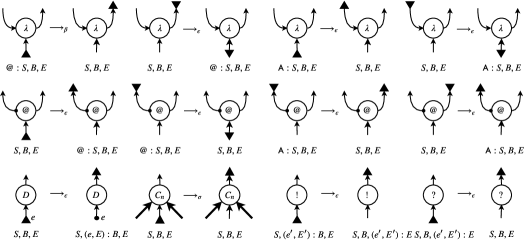
Jump transition: $((G,e),(\mathord{\downarrow},S,B,(e^{\prime},E^{\prime}):E))\to_{\epsilon}((G,e^{\prime}),(\mathord{\downarrow},S,B,E^{\prime}))$, where the old position $e$ is the output of a $\mathop{!}$-node: .

Given a term $t$ with the call-by-need function application ($@$) abused, a successful execution $((t^{\dagger},e_{t}),(\mathord{\uparrow},\square,\square,\square,\square))\to^{*}((t^{\dagger},e_{v}),(\mathord{\uparrow},\square,\square,\square,\square))$ starts at the root $e_{t}$ of the translation $t^{\dagger}$, and ends at the root $e_{v}$ of the translation $v^{\dagger}$, for some sub-value $v$ of the term $t$. The value $v$ indicates the evaluation result.

Figure 17. Passes-Only DGoIM plus Jumping for Call-by-Name [DR96]

Finally, we give a quantitative comparison of space usage between rewriting and jumping. As a case study, we focus on implementations of call-by-name/need evaluation, namely on the passes-only DGoIM recalled in Fig. 16, our rewrites-first DGoIM, and the passes-only DGoIM equipped with jumping that we will recall in Fig. 17. A similar comparison is possible for left-to-right call-by-value evaluation, between our rewrites-first DGoIM and the jumping machine given by Fernández and Mackie [FM02].

Fig. 17 recalls Danos and Regnier’s token-passing machine equipped with jumping [DR96], which is proved to be isomorphic to Krivine’s abstract machine [Kri07] for call-by-name evaluation. The machine has pass transitions as well as the jump transition that lets the token jump to a remote position. Compared with the token-passing GoI (Fig. 16), pass transitions for nodes related to $\mathop{!}$-boxes are reduced and changed, so that the jumping mechanism imitates rewrites involving $\mathop{!}$-boxes. The token remembers its old position, together with its current environment stack, when passing a $\mathit{D}$-node upwards. The token uses this information and make a jump back in the jump transition, in which the token exits a $\mathop{!}$-box at the principal door ($\mathop{!}$-node) and changes its position to the remembered link $e^{\prime}$.

The quantitative comparison, whose result is stated below, shows partial duplication of token data impacts space usage much more than duplication of sub-graphs, and therefore rewriting has asymptotically better space usage than jumping.

Proposition 10.

After $n$ transitions from an initial state of a graph of size $|G_{0}|$, space usage of three versions of the DGoIM is bounded as in the table below.

machines	token-passing only	rewriting added	jumping added
	(Fig. 16)	(Fig. 5 & Fig. 6)	(Fig. 17)
evaluations implemented	call-by-name	call-by-need	call-by-name
size of graph	$|G_{0}|$	$\mathcal{O}(n\cdot|G_{0}|)$	$|G_{0}|$
size of token position	$\log{|G_{0}|}$	$\mathcal{O}{(\log{(n\cdot|G_{0}|)})}$	$\log{|G_{0}|}$
size of token data	$\mathcal{O}(n\cdot\log{|G_{0}|})$	$\mathcal{O}(n\cdot\log{(n\cdot|G_{0}|)})$	$\mathcal{O}(2^{n}\cdot\log{|G_{0}|})$

Proof 6.1.

The size $|G_{n}|$ of the underlying graph after $n$ transitions can be estimated using the size $|G_{0}|$ of the initial graph. Our rewrites-first DGoIM is the only one that changes the underlying graph during an execution. Thanks to the sub-graph property (Lem. 3), the size $|G_{n}|$ can be bounded as $|G_{n}|=\mathcal{O}(n_{\sigma}\cdot|G_{0}|)$, where $n_{\sigma}$ is the number of $\sigma$-labelled transitions in the $n$ transitions. In the token-passing machines with and without jumping (Fig. 16 and Fig. 17), clearly $|G_{n}|=|G_{0}|$. In any of the three machines, the token position can be represented in the size of $\log{|G_{n}|}$.

Next estimation is of token data. Because stacks can have a link of the underlying graph as an element, the size of token data after $n$ transitions depends on $\log{|G_{n}|}$. Both in the token-passing machine (Fig. 16) and our rewrites-first DGoIM, at most one element is pushed in each transition. Therefore the size of token data is bounded by $n\cdot\mathcal{O}(\log{(|G_{n}|)})$. On the other hand, in the jumping machine (Fig. 17), the size of token data, especially the box stack and the environment stack, can grow exponentially because of the partial duplication. Therefore token data has the size $\mathcal{O}(2^{n}\cdot\log{(|G_{n}|)})$. For example, a term with many $\eta$-expansions, like $(\lambda{f}.(\lambda{x}.(\lambda{y}.(\lambda{z}.f\,z)\,y)\,x))\,(\lambda{w}.w)$, causes exponential grow of the box stack in the jumping machine.

7. Related Work and Conclusion

In an abstract machine of any functional programming language, computations assigned to variables have to be stored for later use. Potentially multiple, conflicting, computations can be assigned to a single variable, primarily because of multiple uses of a function with different arguments. Different solutions to this conflict lead to different representations of the storage, some of which are examined by Accattoli and Barras [AB17] from the perspective of time-cost analysis. We recall a few solutions below that seem relevant to our token-guided graph-rewriting.

One solution is to allow at most one assignment to each variable. This is typically achieved by renaming bound variables during execution, possibly symbolically. Examples for call-by-need evaluation are Sestoft’s abstract machines [Ses97], and the storeless and store-based abstract machines studied by Danvy and Zerny [DZ13]. Our graph-rewriting abstract machine gives another example, as shown by the simulation of the sub-machine semantics that resembles the storeless abstract machine mentioned above. Variable renaming is trivial in our machine, thanks to the use of graphs in which variables are represented by mere edges.

Another solution is to allow multiple assignments to a variable, with restricted visibility. The common approach is to pair a sub-term with its own “environment” that maps its free variables to their assigned computations, forming a so-called “closure”. Conflicting assignments are distributed to distinct localised environments. Examples include Cregut’s lazy variant [Cré07] of Krivine’s abstract machine for call-by-need evaluation, and Landin’s SECD machine [Lan64] for call-by-value evaluation. Fernández and Siafakas [FS09] refine this approach for call-by-name and call-by-value evaluations, based on closed reduction [FMS05], which restricts beta-reduction to closed function arguments. This suggests that the approach with localised environments can be modelled in our setting by implementing closed reduction. The implementation would require an extension of rewrite transitions and a different strategy to trigger them, namely to eliminate auxiliary doors of a $\mathop{!}$-box.

Finally, Fernández and Siafakas [FS09] propose another approach to multiple assignments, in which multiple assignments are augmented with binary strings so that each occurrence of a variable can only refer to one of them. This approach is inspired by the token-passing GoI, namely a token-passing abstract machine for call-by-value evaluation, designed by Fernández and Mackie [FM02]. The augmenting binary strings come from paths of trees of binary contractions, which are used by the token-passing machine to represent shared assignments. In our graph-rewriting machine, trees of binary contractions are replaced with single generalised contraction nodes of arbitrary arity, to achieve time efficiency. Therefore, the counterpart of the paths over binary contractions is simply connections over single generalised contraction nodes.

To wrap up, we introduced the DGoIM, which can interleave token-passing GoI with graph rewriting, using the token-passing as a guide. As a case study, we showed how the DGoIM with the rewrites-first interleaving can time-efficiently implement three evaluations: call-by-need, left-to-right call-by-value and right-to-left call-by-value. These evaluations have different control over caching intermediate results. The difference boils down to different routing of the token in the DGoIM, which is achieved by simply switching graph representations (namely, nodes modelling function application) of terms.

The idea of using the token as a guide of graph rewriting was also proposed by Sinot [Sin05, Sin06] for interaction nets. He shows how using a token can make the rewriting system implement the call-by-name, call-by-need and call-by-value evaluation strategies. Our development in this work can be seen as a realisation of the rewriting system as an abstract machine, in particular with explicit control over copying sub-graphs.

The token-guided graph rewriting is a flexible framework with which we can implement various evaluation strategies of the lambda-calculus and analyse execution cost. Our focus in this work was primarily on time efficiency. This is to complement existing work on operational semantics given by token-passing GoI, which usually achieves space efficiency, and also to confirm that introduction of graph rewriting to the semantics does not bring in any hidden inefficiencies. We believe that further refinements, not only of the interleaving strategies of token routing and graph reduction, but also of the graph representation, can be formulated to serve particular objectives in the space-time execution efficiency trade-off, such as full lazy evaluation, as hinted by Sinot [Sin05].

As a final remark, the flexibility of our framework also allows us to handle the operational semantics of exotic language features, especially data-flow features. One such feature is to turn a parametrised data-flow network into an ordinary function that takes parameters as an argument and returns the network, which we model using the token-guided graph rewriting [CDG⁺18]. This feature can assist a common programming idiom of machine learning tasks, in which a data-flow network is constructed as a program, and then modified at run-time by updating values of parameters embedded into the network.

References

- [AB17] Beniamino Accattoli and Bruno Barras. Environments and the complexity of abstract machines. In PPDP 2017, pages 4–16. ACM, 2017.
- [ABM14] Beniamino Accattoli, Pablo Barenbaum, and Damiano Mazza. Distilling abstract machines. In ICFP 2014, pages 363–376. ACM, 2014.
- [Acc17] Beniamino Accattoli. The complexity of abstract machines. In WPTE 2016, volume 235 of EPTCS, pages 1–15, 2017.
- [AD16] Beniamino Accattoli and Ugo Dal Lago. (leftmost-outermost) beta reduction is invariant, indeed. Logical Methods in Comp. Sci., 12(1), 2016.
- [AG09] Beniamino Accattoli and Stefano Guerrini. Jumping boxes. In CSL 2009, volume 5771 of Lect. Notes Comp. Sci., pages 55–70. Springer, 2009.
- [AK10] Beniamino Accattoli and Delia Kesner. The structural -calculus. In CSL 2010, volume 6247 of Lect. Notes Comp. Sci., pages 381–395. Springer, 2010.
- [AS14] Beniamino Accattoli and Claudio Sacerdoti Coen. On the value of variables. In WoLLIC 2014, volume 8652 of Lect. Notes Comp. Sci., pages 36–50. Springer, 2014.
- [CDG+18] Steven W. T. Cheung, Victor Darvariu, Dan R. Ghica, Koko Muroya, and Reuben N. S. Rowe. A functional perspective on machine learning via programmable induction and abduction. In FLOPS 2018, volume 10818 of Lect. Notes Comp. Sci., pages 84–98. Springer, 2018.
- [Cré07] Pierre Crégut. Strongly reducing variants of the Krivine abstract machine. Higher-Order and Symbolic Computation, 20(3):209–230, 2007.
- [DFVY15] Ugo Dal Lago, Claudia Faggian, Benoît Valiron, and Akira Yoshimizu. Parallelism and synchronization in an infinitary context. In LICS 2015, pages 559–572. IEEE, 2015.
- [DFVY17] Ugo Dal Lago, Claudia Faggian, Benoît Valiron, and Akira Yoshimizu. The Geometry of Parallelism: classical, probabilistic, and quantum effects. In POPL 2017, pages 833–845. ACM, 2017.
- [DG11] Ugo Dal Lago and Marco Gaboardi. Linear dependent types and relative completeness. In LICS 2011, pages 133–142. IEEE Computer Society, 2011.
- [DMMZ12] Olivier Danvy, Kevin Millikin, Johan Munk, and Ian Zerny. On inter-deriving small-step and big-step semantics: a case study for storeless call-by-need evaluation. Theor. Comp. Sci., 435:21–42, 2012.
- [DP12] Ugo Dal Lago and Barbara Petit. Linear dependent types in a call-by-value scenario. In PPDP 2012, pages 115–126. ACM, 2012.
- [DR96] Vincent Danos and Laurent Regnier. Reversible, irreversible and optimal lambda-machines. Elect. Notes in Theor. Comp. Sci., 3:40–60, 1996.
- [DS16] Ugo Dal Lago and Ulrich Schöpp. Computation by interaction for space-bounded functional programming. Inf. Comput., 248:150–194, 2016.
- [DZ13] Olivier Danvy and Ian Zerny. A synthetic operational account of call-by-need evaluation. In PPDP 2013, pages 97–108. ACM, 2013.
- [FM02] Maribel Fernández and Ian Mackie. Call-by-value lambda-graph rewriting without rewriting. In ICGT 2002, volume 2505 of LNCS, pages 75–89. Springer, 2002.
- [FMS05] Maribel Fernández, Ian Mackie, and François-Régis Sinot. Closed reduction: explicit substitutions without alpha-conversion. Math. Struct. in Comp. Sci., 15(2):343–381, 2005.
- [FS09] Maribel Fernández and Nikolaos Siafakas. New developments in environment machines. Elect. Notes in Theor. Comp. Sci., 237:57–73, 2009.
- [Ghi07] Dan R. Ghica. Geometry of Synthesis: a structured approach to VLSI design. In POPL 2007, pages 363–375. ACM, 2007.
- [Gir87] Jean-Yves Girard. Linear logic. Theor. Comp. Sci., 50:1–102, 1987.
- [Gir89] Jean-Yves Girard. Geometry of Interaction I: interpretation of system F. In Logic Colloquium 1988, volume 127 of Studies in Logic & Found. Math., pages 221–260. Elsevier, 1989.
- [GS11] Dan R. Ghica and Alex Smith. Geometry of Synthesis III: resource management through type inference. In POPL 2011, pages 345–356. ACM, 2011.
- [GSS11] Dan R. Ghica, Alex Smith, and Satnam Singh. Geometry of Synthesis IV: compiling affine recursion into static hardware. In ICFP, pages 221–233, 2011.
- [HMH14] Naohiko Hoshino, Koko Muroya, and Ichiro Hasuo. Memoryful Geometry of Interaction: from coalgebraic components to algebraic effects. In CSL-LICS 2014, pages 52:1–52:10. ACM, 2014.
- [Kis12] Aleks Kissinger. Pictures of processes: automated graph rewriting for monoidal categories and applications to quantum computing. CoRR, abs/1203.0202, 2012.
- [Kri07] Jean-Louis Krivine. A call-by-name lambda-calculus machine. Higher-Order and Symbolic Computataion, 20(3):199–207, 2007.
- [Lan64] Peter Landin. The mechanical evaluation of expressions. The Comp. Journ., 6(4):308–320, 1964.
- [Mac95] Ian Mackie. The Geometry of Interaction machine. In POPL 1995, pages 198–208. ACM, 1995.
- [Mel06] Paul-André Melliès. Functorial boxes in string diagrams. In CSL 2006, volume 4207 of Lect. Notes Comp. Sci., pages 1–30. Springer, 2006.
- [MG17a] Koko Muroya and Dan R. Ghica. The dynamic Geometry of Interaction machine: a call-by-need graph rewriter. In CSL 2017, volume 82 of LIPIcs, pages 32:1–32:15, 2017.
- [MG17b] Koko Muroya and Dan R. Ghica. Efficient implementation of evaluation strategies via token-guided graph rewriting. In WPTE 2017, 2017.
- [MHH16] Koko Muroya, Naohiko Hoshino, and Ichiro Hasuo. Memoryful Geometry of Interaction II: recursion and adequacy. In POPL 2016, pages 748–760. ACM, 2016.
- [MOTW99] John Maraist, Martin Odersky, David N. Turner, and Philip Wadler. Call-by-name, call-by-value, call-by-need and the linear lambda calculus. Theor. Comp. Sci., 228(1-2):175–210, 1999.
- [Sch11] Ulrich Schöpp. Computation-by-interaction with effects. In APLAS 2011, volume 7078 of Lect. Notes Comp. Sci., pages 305–321. Springer, 2011.
- [Sch14a] Ulrich Schöpp. Call-by-value in a basic logic for interaction. In APLAS 2014, volume 8858 of Lect. Notes Comp. Sci., pages 428–448. Springer, 2014.
- [Sch14b] Ulrich Schöpp. Organising low-level programs using higher types. In PPDP 2014, pages 199–210. ACM, 2014.
- [Ses97] Peter Sestoft. Deriving a lazy abstract machine. J. Funct. Program., 7(3):231–264, 1997.
- [Sin05] François-Régis Sinot. Call-by-name and call-by-value as token-passing interaction nets. In TLCA 2005, volume 3461 of Lect. Notes Comp. Sci., pages 386–400. Springer, 2005.
- [Sin06] François-Régis Sinot. Call-by-need in token-passing nets. Math. Struct. in Comp. Sci., 16(4):639–666, 2006.