Lattice Boltzmann model approximated

with finite difference expressions

François Dubois^a,b, Pierre Lallemand^c,

Christian Obrecht^d and Mohamed Mahdi Tekitek^e

^a Conservatoire National des Arts et Métiers,

Laboratoire de Mécanique des Structures et des Systèmes Couplés, F-75003, Paris, France

^b Department of Mathematics, University Paris-Sud, Bât. 425, F-91405 Orsay Cedex, France.

^c Beijing Computational Science Research Center,

Zhanggguancun Software Park II, Haidian District, Beijing 100094, China.

^d Institut National des Sciences Appliquées de Lyon,

Centre d’Énergétique et de Thermique de Lyon (UMR 5008),

Campus La Doua - LyonTech, 69621 Villeurbanne Cedex, France.

^e Department of Mathematics, Faculty of Sciences,

University of Tunis El Manar, 2092, Tunis, Tunisia

francois.dubois@math.u-psud.fr, christian.obrecht@insa-lyon.fr,

pierre.lallemand1@free.fr, mohamedmahdi.tekitek@fst.rnu.tn

16 April 2016

Abstract.   We show that the asymptotic properties of the link-wise artificial compressibility method are not compatible with a correct approximation of fluid properties. We propose to adapt the previous method through a framework suggested by the Taylor expansion method and to replace first order terms in the expansion by appropriate three or five points finite differences and to add non linear terms. The “FD-LBM” scheme obtained by this method is tested in two dimensions for shear wave, Stokes modes and Poiseuille flow. The results are compared with the usual lattice Boltzmann method in the framework of multiple relaxation times.

Keywords: artificial compressibility method, quartic parameters.
PACS numbers: 02.70.Ns, 05.20.Dd, 47.10.+g, 47.11.+j.
Mathematics Subject Classification (2010): 76M28.

Introduction

Lattice Boltzmann models (LBM) make it possible to simulate various types of fluid flows with simple algorithms (see e.g. [4, 5, 14, 18, 19]). Usually one can observe (and in simple cases, prove) second order accuracy (see e.g. [13]). These features make LBM approaches increasingly popular for engineering applications besides others. However, unlike standard simulation methods such as finite differences, lattice Boltzmann models are required to process more information than the primitive hydrodynamic variables, which leads to higher memory consumption and larger data throughput per collocation point.

On modern computers, especially when using massively parallel processors such as graphics processing units (GPUs), the computational performance of the LBM is memory-bound, and therefore is directly linked to the size of the stencil associated to each collocation point. Asinari et al. [1, 15, 16, 17] proposed the link-wise artificial compressibility method (LW-ACM) in which parts of the LBM algorithm are replaced by expressions deduced from finite differencing the primitive variables and gave some results that looked quite encouraging. Compared to standard three-dimensional LBM, the LW-ACM reduces memory consumption by a factor of 4.75 and increases performance of GPU implementations by approximately by a factor of 1.8 [15].

We present an analysis of some features of the link-wise artificial compressibility method of Asinari et al., showing possible flaws and then propose alternative finite difference expressions that allow a significant improvement of the resulting simulations.

1)  Definition of the models

For the sake of simplicity, we start from the usual D2Q9 lattice Boltzmann model [14] that allows us to simulate weakly compressible Navier-Stokes flows. Using a planar square grid with collocation points located at $x_{ij}=i\ \delta x$, $y_{ij}=j\ \delta x$, a fluid is represented by 9 real quantities $f_{ij}^{n}$ at each of these grid points. The LBM simulations involve two steps (collision and propagation) that we describe following d’Humières [11, 12]. For the collision at each grid point, one makes a linear transformation of the quantities $f$ to moments $m$ using an orthogonal matrix $\cal M$ which is shown below together with a physical interpretation :

$\rho$	1	1	1	1	1	1	1	1	1	density
$J_{x}$	0	1	0	1	0	1	-1	-1	1	mass flux
$J_{y}$	0	0	1	0	1	1	1	-1	-1	mass flux
$E$	-4	-1	-1	-1	-1	2	2	2	2	energy
$XX$	0	1	-1	1	-1	0	0	0	0	diagonal stress
$XY$	0	0	0	0	0	1	-1	1	-1	off-diagonal stress
$q_{x}$	0	-2	0	2	0	1	-1	-1	1	energy flux
$q_{y}$	0	0	-2	0	2	1	1	-1	-1	energy flux
$\epsilon$	4	-2	-2	-2	-2	1	1	1	1	square of energy

Depending on the simulations to be done, we can conserve only the first moment to solve thermal-like problems or we can conserve the three first moments to solve fluid problems for two-dimensional space. The others (non conserved) are assumed to evolve as

(1) $$m_{k}^{*}=m_{k}+s_{k}(m_{k}^{eq}-m_{k}),$$

where $m_{k}^{eq}$ is an equilibrium value that is a function of the conserved moments and $s_{k}$ a relaxation rate. Note that symmetry considerations are useful to propose expressions for these equilibrium values.

The post-collision moments can also be modified by an external force (gravity, Coriolis, etc..), preferably following the splitting of Strang [6] : applying half of the perturbation before collision and half after. Once the new moments are known, applying ${\cal M}^{-1}$ leads to post-collision $f^{n*}$. Propagation is simply obtained through

(2) $$f^{n+1}_{i_{0}j_{0}}=f^{n*}_{ij},$$

where $i_{0}$ and $j_{0}$ are indices of the neighboring grid point corresponding to the elementary velocity used to define the moments $J_{x}$ and $J_{y}$. Thus, once a velocity set has been chosen, the “adjustable” parameters of a LBM model are the expressions of the equilibrium values of the non-conserved moments and the values of the relaxation rates.

The analysis of a LBM simulation can be done in several ways. The most popular is a second order analysis based on the Chapman-Enskog development used in the kinetic theory of classical gases (see e.g. [11] or [14]). This allows to compute the kinematic transport coefficients (diffusivity for just one conserved moment, shear and bulk viscosities for three conserved moments). It also gives first order expressions for the non-conserved moments. More recently it was proposed to obtain equivalent equations through Taylor’s expansions [2, 7, 8], which allow to study the effect of higher order space derivatives in a much simpler way than does the Chapman-Enskog development (which makes use of non commuting matrix products). Finally using the dispersion equation allows to study the linear stability and gives all the information needed to evaluate the properties of a simulation model.

1-a)  Standard D2Q9

The standard D2Q9 [14] model for Navier-Stokes uses the following parameters

moment		equilibrium	rate
E	=	$-2\rho+3(J_{x}^{2}+J_{y}^{2})/\rho$	$s_{e}$
XX	=	$(J_{x}^{2}-J_{y}^{2})/\rho$	$s_{xx}$
XY	=	$(J_{x}\ J_{y})/\rho$	$s_{xx}$
$q_{x}$	=	$-J_{x}$	$s_{q}$
$q_{y}$	=	$-J_{y}$	$s_{q}$
$\epsilon$	=	$\rho-3(J_{x}^{2}+J_{y}^{2})/\rho$	$s_{\epsilon}$

This leads to the following properties :

speed of sound	$c_{s}$	=	$\sqrt{\frac{1}{3}}$,
kinematic shear viscosity	$\nu$	=	$\frac{1}{3}(\frac{1}{s_{xx}}-\frac{1}{2})$,
kinematic bulk viscosity	$\zeta$	=	$\frac{1}{3}(\frac{1}{s_{e}}-\frac{1}{2}).$

The non linear terms lead to the correct advection of shear and acoustic waves. However, in advective acoustics framework where a uniform velocity $V$ is given, the LBM method computes the deviation from this given advection. A linear analysis show that low amplitude shear waves with wave vector parallel to $V$ are damped with an effective kinematic shear viscosity

$$\nu_{\textit{eff}}=\nu\ (1\ -3\ V^{2}).$$

The correction is significant as $V$ may be as large as $\,0.2$ that is typically up to $\,0.35\,$ times the sound speed $c_{s}.$ In the absence of a large velocity, one can easily get higher order terms in the equivalent equations which allows to determine a shear “hyperviscosity” from the attenuation rate of shear waves at order four in space derivatives. Previous work [2, 9, 10] showed which conditions allowed to get an isotropic hyperviscosity (no angular dependence in the expressions) and the possibility to make it equal to zero.

1-b)  Link-wise artificial compressibility method

The new proposal of Asinari et al. [1, 15, 16, 17] uses just the primitive variables: density $\rho$ and velocity $\vec{u}$. From these quantities it reconstructs a set of $f^{n}$ on all grid points of the computation domain and then lets them evolve with the LBM rules. In its original formulation, the reconstruction rule is expressed through the equilibrium distribution $f^{eq}$ which is function of the sole primitive variables. Using the present notations, it can be written as:

(3) $$f^{n*}_{ij}=f^{eq}(\rho^{n}_{ij},\vec{u}^{\,n}_{ij})+\Theta\left(f^{eo}(\rho^{n}_{i_{0}j_{0}},\vec{u}^{\,n}_{i_{0}j_{0}})-f^{eo}(\rho^{n}_{ij},\vec{u}^{\,n}_{ij})\right)\,,$$

where $f^{eo}(\rho,\vec{u})$ is defined as:

$$f^{eo}(\rho,\vec{u})=\frac{1}{2}\left(f^{eq}(\rho,\vec{u})-f^{eq}(\rho,-\vec{u})\right)\,,$$

and $\Theta$ as:

$$\Theta=1-\frac{2\nu}{c_{s}^{2}}=1-6\nu\,.$$

The properties of the proposed algorithm lies in the reconstitution. The work of Asinari et al. use what can be called “zeroth-order” reconstitution as they just involve the expressions shown in the preceding table.

To analyze it we use a classical Von Neumann stability analysis in Fourier space (see [14]). So we proceed in the following way. Starting either from the equations to be simulated or from the computer code derived from them we prepare a series of instructions for a computer algebra system. We then consider a grid with the following initial conditions : a plane wave of small amplitude and wave vector $k_{x},\ k_{y}$, uniform density plus possibly a uniform velocity $V=(V_{x},V_{y}).$ This means we take the following initial state : $f=f^{0}+\delta f$, where $f^{0}=(f_{0},\dots,f_{8})$ represents the uniform equilibrium state specified by uniform and steady density $\rho$ and velocity $V=(V_{x},V_{y})$ and $\delta f=(\delta f_{0},\dots,\delta f_{8})$ is the fluctuation. We then apply one time step in the Fourier space and linearize the results in terms of the parameters of the plane wave (amplitude and phase factors).

We define space phase factors $p=e^{i\,k_{x}}$ and $q=e^{i\,k_{y}}$ and time factor $z=e^{-\Gamma}$ ($i$ is unit imaginary number and $\Gamma$ being the attenuation rate) in units such that $\delta x=1$ and the duration of one time step equals to unity. So the initial conditions in moment space are

$$\delta\rho(j,l)\,=\,A\ p^{j}\ q^{l}\,,\quad\delta J_{x}(j,l)\,=\,B\,p^{j}\ q^{l}\,,\quad\delta J_{y}(j,l)\,=\,C\ p^{j}\ q^{l}.$$

In consequence we have classical relation of the type

$$\delta\rho(j+1,l)=e^{ik_{x}}\,\delta\rho(j,l)=p\,\delta\rho(j,l),\quad\delta\rho(j,l+1)=e^{ik_{y}}\,\delta\rho(j,l)=q\,\delta\rho(j,l),$$

and analogous relations for two others fields $\delta J_{x}$ and $\delta J_{y}.$ We introduce the state vector $\Phi=\left(A,B,C\right)^{{\rm{t}}}$, after one time step the vector $\Phi$ is multiplied by the amplification matrix $H$ :

(4) $$\Phi^{n+1}=H\,\Phi^{n}.$$

We note here that the amplification matrix $H$ is determined by the collision step and the advection step. In particular the coefficients : $V$, $c_{s}$, $s_{k}$, $p$ and $q$ (see for details the original reference [14]). $\Phi=\left(\delta\rho,\ \delta J_{x},\ \delta J_{y}\right)^{{\rm{t}}}$ We search the modes associated to the iteration (4). In that case the vector $\Phi$ is solution of

(5) $$z\ \Phi=H\ \Phi\,,$$

from which we get the dispersion equation

(6) $$F(p,q,z)=\det(H-z\ Id)\,,$$

where $Id$ is the unit matrix. Literal expressions of $F$ are then solved to get $z$ by successive approximations in powers of the wave vector components. In other terms we search the eigenvalues $z$ and eigenvectors $R$ as powers of the wave vector $(k_{x},k_{y}).$ So that the attenuation rate (possibly complex for propagating waves) is obtained as an expansion in wave vector components with $\Gamma=\log{z}$. As the general expressions are quite cumbersome, we only give information on the terms up to power 2 in wave vector components. In addition we assume that the uniform velocity is parallel to the wave vector with amplitude $v$ (i.e. $V=(V_{x},V_{y})$ and $v=|V|$) and we apply a rotation of the axis so that the wave vector is parallel to Ox (rotated axis) with amplitude $k$. We replace the spatial phase factor $p$ and $q$ by their expansion at second order in in $k$. We then get the matrix $H(k)$ :

$$H(k)\,=\,\left(\begin{array}[]{ccc}1-6\,i\,vk\nu-\frac{1}{6}k^{2}(1+3v^{2})&-6\,i\,\nu k-vk^{2}&0\cr-\frac{1}{3}\,i\,k(1+3v^{2})+v(1-3vk^{2})&1-2\,i\,kv-3\nu k^{2}&0\cr 0&0&1-\,i\,kv-\nu k^{2}\end{array}\right).$$

Note that no angle appears, so the model is isotropic at order 2 in wave vector. The previous matrix shows decoupling of one shear mode and two longitudinal modes.

From the roots of the dispersion equation in the case $v=0$, one obtains the kinematic shear viscosity $\nu$, related to the relaxation rate $s_{xx}$ by

$$\nu=\frac{1}{3}\,\Big{(}\frac{1}{s_{xx}}-\frac{1}{2}\Big{)}\,,$$

and the speed of sound and its damping

$$c_{s}=\sqrt{2\nu},\quad\ \Gamma_{s}=\frac{\nu}{2}+\frac{1}{12}\,.$$

Note that the result for the damping of sound can be interpreted with a kinematic bulk viscosity independent of the parameters of the model.

When $v$ is not zero, since the transport coefficients can be obtained through a perturbation analysis, we shall use the following series expansion in $k$ of the roots [14]. One can verify that the roots contain a linear dependence in $v$ (term in $\,ikv$ linked to linear advection) and the shear viscosity becomes

$$\nu(v)=\nu-\frac{1}{2}\ v^{2}\,.$$

This last result means that if $v>\sqrt{2\nu}\ =\ c_{s}$, shear waves grow exponentially and thus the model is unstable so it is not recommended to use this model for simulations at fairly large Reynolds number. Actual simulations allow to verify the previous results (see section 3-a)

2)  New proposition

We propose to use the same basic idea (reconstruction of the $f$ from primitive variables : density, components of the velocity), but with improved formulae.

In the Taylor expansion analysis leading to the equivalent equations [7], it was shown that the non conserved moments $m_{k}$ can be expanded in powers of the size of the elementary step of the algorithm. Beyond the order 0, presented above, the second order has been expressed in terms of $\theta_{k}$ that involve space derivatives and non linear terms. In fact, as described in [7], we have the following development of non-equilibrium moments at second order on $\Delta t$ :

(7) $$m_{k}^{*}=m_{k}^{eq}+\Delta t\left(\frac{1}{2}-\sigma_{k}\right)\theta_{k}+{\rm{O}}(\Delta t^{2}),\quad k\geq 2.$$

where $\sigma_{k}\equiv\left(\frac{1}{s_{k}}-\frac{1}{2}\right)$ and $\theta_{k}$ is the defect of conservation defined by :

(8) $$\theta_{k}\equiv\partial_{t}m_{k}^{eq}+\Lambda_{k\,\alpha}^{\ell}\partial_{\alpha}m_{\ell},\quad k>N,$$

where $N$ is the number of the conserved moments and $\Lambda_{k\,\alpha}^{\ell}=\sum_{j}v_{j}^{\alpha}v_{j}^{\beta}(M^{-1})_{jk}$, $k=0\dots 8$, $\alpha=1\dots 2$ and $\beta=1\dots 2$.
Remark In the case of the $N=3$ (i.e. 3 conserved moment to model fluid-like problems), we get the following macroscopic equations :

$$\partial_{t}m_{k}+\Lambda_{k\,\alpha}^{\ell}\,\partial_{\alpha}m_{\ell}^{eq}-\sigma_{\ell}\,\Delta t\,\Lambda_{k\,\alpha}^{\ell}\,\partial_{\alpha}\theta_{\ell}={\rm{O}}(\Delta t)^{2},\quad k=0,1,2.$$

We note here that for $k=1,2$ at the order one we have a term $\frac{1}{3}\nabla\rho$ which gives the sound speed $c_{s}=\frac{1}{\sqrt{3}}.$ At the order two (terms having $\Delta t$ as coefficient) we obtain the viscous terms function of $\sigma_{\ell}$. For more details see [7].

As many individual terms are found to play no role in the behavior of the shear and acoustic modes, we give only the relevant terms of the defect of conservation $\theta_{k}$ (8) for the case where the density is close to 1 :

$$\left\{\begin{array}[]{lcccl}\theta_{3}&\equiv&\theta_{E}&=&(2+6\ (v_{x}^{2}+v_{y}^{2}))\ (\partial_{x}v_{x}+\partial_{y}v_{y})-2\ (v_{x}\partial_{x}\rho+v_{y}\partial_{y}\rho),\\ \theta_{4}&\equiv&\theta_{XX}&=&\frac{2}{3}(\partial_{x}v_{x}-\partial_{y}v_{y})-\frac{2}{3}(v_{x}\partial_{x}\rho-v_{y}\partial_{y}\rho)\\ &&&&\qquad-\,2(v_{x}(\partial_{x}v_{x}^{2}+\partial_{y}v_{x}v_{y})-v_{y}(\partial_{x}v_{x}v_{y}+\partial_{y}v_{y}^{2}),\\ \theta_{5}&\equiv&\theta_{XY}&=&\frac{1}{3}(\partial_{x}v_{y}-\partial_{y}v_{x})-\frac{1}{3}(v_{x}\partial_{y}\rho+v_{y}\partial_{x}\rho)\\ &&&&\qquad-\,v_{x}(\partial_{x}v_{x}v_{y}+\partial_{y}vy^{2})-v_{y}(\partial_{x}v_{x}^{2}+\partial_{y}v_{x}v_{y})\,.\end{array}\right.$$

The partial derivatives are then estimated by finite difference. To sum up, the neighboring $f$ are obtained (see equation (7)) using the non-conserved moments :

$$\left\{\begin{array}[]{lcl}E&=&-2\rho+3(v_{x}^{2}+v_{y}^{2})/\rho+(1-\frac{1}{s_{e}})\ \theta_{E},\\ XX&=&(J_{x}^{2}-J_{y}^{2})/\rho+(1-\frac{1}{s_{xx}})\ \theta_{XX},\\ XY&=&(J_{x}\ J_{y})/\rho+(1-\frac{1}{s_{xx}})\ \theta_{XY},\\ q_{x}&=&-J_{x},\\ q_{y}&=&-J_{y},\\ \epsilon&=&\rho-3(v_{x}^{2}+v_{y}^{2})/\rho.\\ \end{array}\right.$$

With these expressions, the acoustic waves propagate with speed $1/\sqrt{3}$ (as for standard D2Q9), advection by a mean velocity $V$ is correct and the viscosities are now :

$$\mbox{shear }=\frac{1}{3}(\frac{1}{s_{xx}}-\frac{1}{2})\ (1-3\ V^{2})\quad\mbox{ and }\quad\mbox{ bulk }=\frac{1}{3}(\frac{1}{s_{e}}-\frac{1}{2})\ (1-3\ V^{2}),$$

as is known for D2Q9.

For the particular case with $V=0$, one can determine higher order contributions to the damping of the hydrodynamic modes. We first expand the dispersion equation (6), then we replace spatial phase factors $p$ and $q$ by their expansions up to the fourth order in $k$ and solve the resulting expression by successive approximation in $k$. This leads to eigenvalues $z_{i},\,i=1..3$ and then we get the development of the damping coefficient $\Gamma_{i}=-\log(z_{i})$. We interpret one of these roots as

$$\Gamma_{i}=\nu_{0}k^{2}+\nu_{2}\,k^{4}.$$

Which allows to define a $k$ dependent kinematic shear viscosity :

$$\nu(k)=\nu_{0}+\nu_{2}\,k^{2},$$

We define the coefficient $\nu_{2}$ as “hyperviscosity”. The expressions for this hyperviscosity depend on the way space derivatives are estimated using finite difference.

We have considered three cases.

$\bullet$  Three points stencil  such that

$$\partial_{x}\bullet\,\simeq\,\frac{1}{2}\,\big{(}\bullet(i+1,j)-\bullet(i-1,j)\big{)}\,.$$

Then the shear hyperviscosity is

$$\nu_{2}=\frac{1}{72}(2\sigma_{xx}-3)(2\sigma_{xx}-1)-\frac{8\sigma_{xx}-3}{36}(\cos{\phi}^{2}-\cos{\phi}^{4}),$$

where $\sigma_{xx}=1/s_{xx}-1/2$ and $\phi$ is the angle between the Ox axis and the wave vector. This contribution is anisotropic. It becomes larger than the usual viscous term for $k>0(\sqrt{\sigma_{xx}})$ which will prevent from doing significant simulations at small viscosity.

$\bullet$  Five points stencil  such that

$$\partial_{x}\bullet\,\simeq\,\frac{3}{4}\,\big{(}\bullet(i+1,j)-\bullet(i-1,j)\big{)}\,-\,\frac{1}{8}\,\big{(}\bullet(i+2,j)-\bullet(i-2,j)\big{)}\,.$$

This leads to a shear hyperviscosity

$$\frac{1}{36}\sigma_{xx}(2\ \sigma_{xx}-1)-\frac{\sigma_{xx}}{18}(\cos{\phi}^{2}-\cos{\phi}^{4}).$$

This is still anisotropic but removes the small viscosity limitation.

$\bullet$  Nine points stencil  based on the D2Q9 geometry, we can use

$$\begin{array}[]{rcl}\partial_{x}\bullet&\,\simeq&\bullet(i+1,j)-\bullet(i-1,j)\\ &\,-&\frac{1}{4}\,\big{[}\bullet(i+1,j+1)-\bullet(i-1,j+1)-\bullet(i-1,j-1)+\bullet(i+1,j-1)\big{]}\end{array}$$

and similar expression for $\partial_{y}$. This leads to the following shear hyperviscosity :

$$\frac{1}{24\ \sigma_{xx}}(3-2\ \sigma_{xx})(2\ \sigma_{xx}-1)-\frac{20\ \sigma_{xx}-9}{12\sigma_{xx}}(\cos{\phi}^{2}-\cos{\phi}^{4})$$

which is still anisotropic and does not solve the limitation indicated for the three point stencil.

For all three stencils, the full dispersion equation (cubic equation in time factor $z$) can be obtained numerically for $k$ up to $\pi$ in order to predict the linear stability.

3)  Results of some simulations

3-a)     Shear wave

Elementary tests have been performed in a square domain (size $N^{2}$) with periodic boundary conditions. The initial condition is a shear wave of wave vector $k_{x},k_{y}$ (of modulus $k$) with in some cases a uniform velocity parallel to the wave vector. In fact we take the following initial conditions :

$$\left\{\begin{array}[]{rcl}\rho(t=0)&=&1,\\ j_{x}(t=0)&=&-A(0)\frac{k_{y}}{k}\cos(k_{x}\,x+k_{x}\,y)+\frac{k_{x}}{k}V,\\ j_{y}(t=0)&=&A(0)\frac{k_{x}}{k}\cos(k_{x}\,x+k_{x}\,y)+\frac{k_{y}}{k}V,\end{array}\right.$$

The exact solution admits the same algebraic form, except that $A$ is replaced by a function of time $A(t)$ ; then $A=A(0)$. At each time step we measure the correlation function $A(t)/A(0)$ of the velocity field with its initial state. For $V=0$, $A(t)$ decays exponentially, otherwise it is $\,e^{(-\Gamma t)}\,\big{(}\cos{\omega t}\big{)}$.

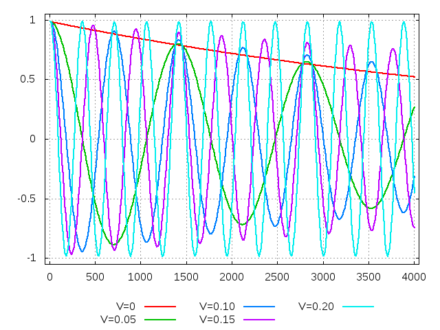
Figure 1: Time evolution of the correlation function $A(t)/A(0)$ versus discrete time between an initial transverse wave (of vector $(3\,k_{0},2\,k_{0})$ where $k_{0}=\frac{2\pi}{191}$) and its later state for five different values of the mean velocity $V$. Square of 191 $\times$ 191 nodes and periodic boundary conditions. When $V$ grows, the dissipation of the waves is reduced.

We show in Fig. 1 the results for the initial ACM model (no $\theta$ in our proposal) for 5 values of the mean velocity $V$. Clearly the velocity square dependence of the damping is unacceptable.

We then perform a series of measurements at $V=0$ for several values of the wave vector and compare (Table 1) the measured relaxation rate $\Gamma$ to the development in terms of hyperviscosity and the numerical root of the dispersion equation (that which corresponds to the transverse mode). Fig. 2, 3 and 4 illustrate the results for the three, five and nine points stencil respectively. These figures have been obtained for a long wave length kinematic shear viscosity $\nu_{0}=0.01$. In the case of the nine point stencil, the model is unstable in the {1,1} direction so no simulation could be performed.

In fact in table 1 we study the equivalent hyperviscosity for the ACM scheme for different stencils. We show that the hyperviscosity is relatively high and negative for an angle equal to $45^{\rm o}$ for the nine point stencil. This is directly correlated to instability in the {1,1} direction.

angle	3-point	5-point	9-point
0.00	0.03725	-0.00103	0.03725
26.60	0.02534	-0.00067	0.00079
45.00	0.01867	-0.00047	-0.0196

Table 1: Numerical study of the hyperviscosity for different stencils of ACM scheme vs angle of the wave vector $k.$ All simulations are performed with the same value $s_{xx}=1.85$.

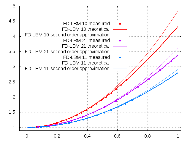
Figure 2: Relative shear viscosity (normalized by $\nu_{0}$) for the three point stencil versus wave vector modulus $k$. Solid curves from dispersion equation, thin solid curves from hyperviscosity, discrete points from actual simulation. Top curves for wave vector along X axis {1,0}, middle curves for wave vector along {2,1} direction and lower curves for wave vector along the {1,1} direction.

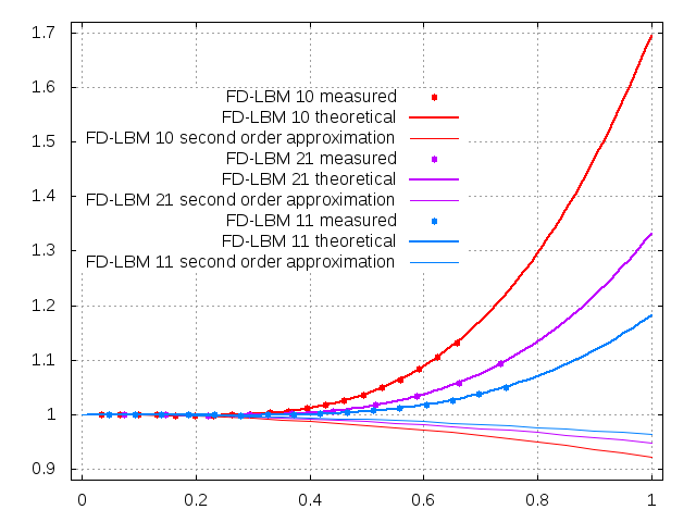
Figure 3: Relative shear viscosity (normalized by $\nu_{0}$) for the five point stencil versus wave vector modulus $k$. Solid curves from dispersion equation, thin solid curves from hyperviscosity, discrete points from actual simulation. Top curves for wave vector along X axis {1,0}, middle curves for wave vector along {2,1} direction and lower curves for wave vector along the {1,1} direction.

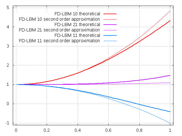
Figure 4: Relative shear viscosity (normalized by $\nu_{0}$) for the nine point stencil versus wave vector modulus $k$. Solid curves from dispersion equation, thin solid curves from hyperviscosity, squares from actual simulation. Top curves for wave vector along X axis, middle curves for wave vector along {2,1} direction and lower curves for wave vector along the {1,1} direction. No experimental data due to linear instability at least in the {1,1} direction.

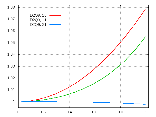
Figure 5: Relative shear viscosity for the D2Q9 lattice Boltzmann model versus wave vector modulus $k$ for three orientations of the wave vector (top {1,0}, middle {2,1}, bottom {1,1}). We observe that the maximal error (8 %) is very much reduced compared to the FD-LBM scheme presented at Figures 2, 3 and 4.

3-b)     Stokes modes

We give some partial results of simulations of situations less elementary that simple plane waves. To take solid boundaries into account we propose to consider the lattice nodes just outside the fluid region and to estimate the state of the virtual fluid in those points by linear extrapolation using the fact that the velocity is 0 on the boundary. As in the scheme of Bouzidi et al.[3] stability is obtained by using different expressions depending on the location of the intersection of the boundary with the link that goes from the last fluid point to the first solid point.

We then compute the relaxation rate of the Stokes modes inside a circle of radius $R=29.9$ lattice units. The flow field is obtained from the stream function

(9) $$\psi(r,\theta,t)=e^{-\big{(}\displaystyle\Gamma\,t\big{)}}\ \cos{(m\ \theta)}J_{n}(r/R),$$

with singlets for $m=0$ and doublets for $m>0$ and

(10) $$\Gamma=\frac{\nu}{R^{2}}\,a_{l}^{2}\,,$$

where $a_{l}$ is a $l^{th}$ zero of the Bessel functions $J_{m}(a_{l})=0$. We give in the following table some values of the relative difference between measured values and the theoretical values for three cases : present FD-LBM with the three point stencil, optimized LBM-D2Q9 ($\nu=1/\sqrt{108}$) and

(11) $$\Big{(}\frac{1}{s_{xx}}-\frac{1}{2}\Big{)}\ \Big{(}\frac{1}{s_{q}}-\frac{1}{2}\Big{)}=\frac{1}{6}\,,$$

required to yield an isotropic hyperviscosity), and a non-optimized D2Q9-LBM (same value of $\nu$, but $s_{q}=1.3$ instead of 0.9282. It is clear that FD-LBM does not match the accuracy of optimized LBM-D2Q9 (see [9]).

$l$	Bessel	FD-LBM-3	FD-LBM-5	BGK	LBE-q
			Singlets
1	14.68200	0.00729	0.00003	0.00053	-0.00010
2	49.21850	0.02191	-0.00141	0.00179	-0.00114
3	103.49950	0.04663	-0.00313	0.00382	-0.00276
4	177.52080	0.07969	-0.00400	0.00672	-0.00489
5	271.28171	0.12335	-0.00358	0.01071	-0.00752
6	384.78189	0.17778	-0.00099	0.01623	-0.01053
			Doublets
1	26.37460	0.01324	-0.00090	0.00106	-0.00042
2	40.70650	0.02078	-0.00103	0.00164	-0.00087
3	57.58290	0.02959	-0.00147	0.00236	-0.00133
4	76.93890	0.03966	-0.00186	0.00323	-0.00183
5	98.72630	0.05060	-0.00231	0.00424	-0.00236
6	122.90760	0.06241	-0.00254	0.00538	-0.00293
7	149.45290	0.07545	-0.00275	0.00667	-0.00354
8	178.33730	0.08948	-0.00267	0.00809	-0.00419
9	209.54010	0.10418	-0.00230	0.00965	-0.00488
10	243.04340	0.12003	-0.00175	0.01138	-0.00563
11	278.83160	0.13682	-0.00099	0.01328	-0.00643

Table 2: Numerical study of the Stokes modes in a disk. All simulations are performed with the same value $\nu_{0}=0.05$. The second column gives the theoretical values and the other the error between the numerical scheme and the theoretical value. The third column uses the present FD-LBM scheme with a three point stencil for the evaluation of the gradients, the fourth column the present FD-LBM scheme with a five point stencil, the fifth column the standard diagonal BGK with $\nu_{0}=0.05$, the sixth column MRT LBM scheme with the quartic condition (11) realized.

$l$	Bessel	FD3-108	FD5-108	BGK-108	LB-108	LB-108-q
			Singlets
1	14.68200	0.00165	-0.00052	0.00069	0.00070	0.00035
2	49.21850	0.00628	-0.00104	0.00179	0.00189	0.00010
3	103.49950	0.01382	-0.00175	0.00355	0.00377	-0.00028
4	177.52080	0.02399	-0.00230	0.00599	0.00640	-0.00078
5	271.28171	0.03665	-0.00244	0.00923	0.00989	-0.00138
6	384.78189	0.05198	-0.00202	0.01341	0.01442	-0.00204
			Doublets
1	26.37460	0.00410	-0.00027	0.00143	0.00147	0.00058
2	40.70650	0.00662	-0.00029	0.00189	0.00197	0.00044
3	57.58290	0.00943	-0.00053	0.00249	0.00262	0.00035
4	76.93890	0.01251	-0.00066	0.00321	0.00339	0.00029
5	98.72630	0.01601	-0.00086	0.00404	0.00428	0.00025
6	122.90760	0.01979	-0.00101	0.00498	0.00530	0.00023
7	149.45290	0.02380	-0.00115	0.00603	0.00643	0.00021
8	178.33730	0.02814	-0.00121	0.00720	0.00768	0.00022
9	209.54010	0.03281	-0.00126	0.00846	0.00905	0.00023
10	243.04340	0.03766	-0.00123	0.00983	0.01053	0.00022
11	278.83160	0.04274	-0.00118	0.01133	0.01215	0.00022

Table 3: Numerical study of the Stokes modes in a disk. All simulations are performed with the same value $\nu_{0}=1/\sqrt{108}$. The second column gives the theoretical values and the other the error between the numerical scheme and the theoretical value. The third column uses the present FD-LBM scheme with a three point stencil for the evaluation of the gradients, the fourth column the present FD-LBM scheme with a five point stencil, the fifth column the standard diagonal BGK with $\nu_{0}=1/\sqrt{108}$, the sixth column the MRT-LBM scheme with the quartic condition (11) not realized and the seventh column the quartic version of the MRT-LBM scheme when the condition (11) is realized.

3-c)     Poiseuille flow

Some simulations of Poiseuille flow have been performed to estimate the efficiency of the boundary conditions. We consider a channel with solid boundaries parallel to the $\,Ox\,$ axis and periodic boundary conditions at the open ends. We adapt the boundary conditions to impose $v=0$ at $y_{1}=1-\xi$ and $y_{2}=N+\xi$. A uniform body force parallel to $\,Ox\,$ drives the flow. After enough time steps the stationary flow is least square fit to a parabolic flow allowing to define “experimental” boundaries where the parabola goes to 0 at $y_{m1}=1-\xi_{m}$ and $y_{m2}=N+\xi_{m}$. We show in Fig. 6 the measured $\xi_{m}$ vs the imposed $\xi$.

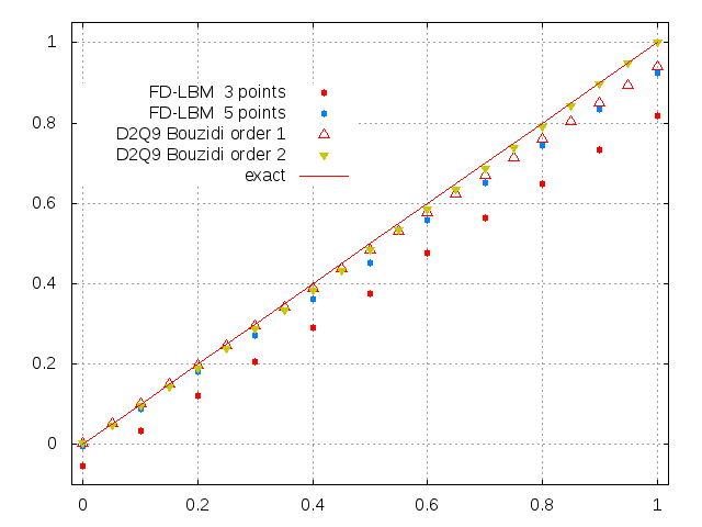
Figure 6: Boundary conditions for a Poiseuille flow. Numerical location of the zero of velocity versus the imposed value $\xi$ of the boundary. In the transverse direction, the computational domain is composed by the interval $\,[1-\xi,\,15+\xi]\,$ where $\,\xi\,$ is the abscissa of the figure. The result is the location of the zero velocity value measured from a least square fit of the velocity profile. The result with the five points difference scheme is of good quality, comparable to what is obtained with the classical D2Q9 usual LBM scheme with first order extrapolation with the Bouzidi et al. algorithm. Observe that with a simple “bounce-back” boundary conditions, the result would be a horizontal line at $\,y=0.5$.

Conclusion

We have shown that the ACM proposal can be improved in two ways : reducing the velocity dependence of the shear viscosity and diminishing the hyperviscosity with the use of a stencil with more points. However when identical values of the long wave length shear and bulk viscosities are chosen for the D2Q9 lattice Boltzmann model, the hyperviscosity is much smaller as can be seen in Fig. 5. An analogous analysis has also been performed for the three-dimensional model D3Q19.

The present work needs to be complemented with detailed testing of situations where nonlinear terms dominate to see the quality of simulations. This will help decide how many grid points in FD-LBM are needed to get comparable accuracy to what is given by a LBE-D2Q9 calculation.

References

References

- [1] P. Asinari, T. Ohwada, E. Chiavazzo, A.F. Di Rienzo. “Link-wise artificial compressibility method”, Journal of Computational Physics, vol. 231, p. 5109-5143, 2012.
- [2] A. Augier, F. Dubois, B. Graille and P. Lallemand. “On rotational invariance of Lattice Boltzmann schemes”, Computers and Mathematics with Applications, vol. 67, p 239-255, 2014.
- [3] M. Bouzidi, M. Firdaous, P. Lallemand, “Momentum transfer of a Boltzmann-lattice fluid with boundaries”, Physics of Fluids, vol. 13, p. 3452-3459, 2001.
- [4] S. Chen, G. D. Doolen. “Lattice Boltzmann method for fluid flows”, Annual Review of Fluid Mechanics, vol. 30, p. 329-364, 1998.
- [5] P. J. Dellar. “Lattice Kinetic Schemes for Magnetohydrodynamics”, Journal of Computational Physics, vol. 179, p. 95-126, 2002.
- [6] P. J. Dellar. “An interpretation and derivation of the lattice Boltzmann method using Strang splitting", Comput. Math. Applic., vol. 65, p. 129-141, 2013.
- [7] F. Dubois. “Equivalent partial differential equations of a Boltzmann scheme”, Computers and mathematics with applications, vol. 55, p. 1441-1449, 2008.
- [8] F. Dubois. “Third order equivalent equation of lattice Boltzmann scheme”, Discrete and Continuous Dynamical Systems-Series A, vol. 23, number 1/2, p. 221-2482009, a special issue dedicated to Ta-Tsien Li on the occasion of his 70th birthday, doi: 10.3934/dcds.2009.23.221, 2009.
- [9] F. Dubois, P. Lallemand. “Towards higher order lattice Boltzmann schemes”, Journal of Statistical Mechanics: Theory and Experiment, P06006 doi: 10.1088/1742-5468/2009/06/P06006, 2009.
- [10] F. Dubois, P. Lallemand. “Quartic Parameters for Acoustic Applications of Lattice Boltzmann Scheme”, Computers and mathematics with applications, vol. 61, p. 3404-3416, 2011, doi:10.1016/j.camwa.2011.01.011.
- [11] D. d’Humières. “Generalized Lattice-Boltzmann Equations”, in Rarefied Gas Dynamics: Theory and Simulations, vol. 159 of AIAA Progress in Astronautics and Astronautics, p. 450-458, 1992.
- [12] D. d’Humières, I. Ginzburg, M. Krafczyk, P. Lallemand and L.S. Luo. “Multiple-relaxation-time lattice Boltzmann models in three dimensions”, Philosophical Transactions of the Royal Society, London, vol. 360, p. 437-451, 2002.
- [13] M. Junk, A. Klar, L.S. Luo. “Asymptotic analysis of the lattice Boltzmann equation”, Journal of Computational Physics, vol. 210, p. 676-704, 2005.
- [14] P. Lallemand, L-S. Luo. “Theory of the lattice Boltzmann method: Dispersion, dissipation, isotropy, Galilean invariance, and stability”, Physical Review E, vol. 61, p. 6546-6562, June 2000.
- [15] C. Obrecht, P. Asinari, F. Kuznik and J.J. Roux. “High-performance implementations and large-scale validation of the link-wise artificial compressibility method”, Journal of Computational Physics, vol. 275, p. 143-153, 2014.
- [16] T. Ohwada, P. Asinari. “Artificial Compressibility Method Revisited: Asymptotic Numerical Method for Incompressible Navier-Stokes Equations”, Journal of Computational Physics, vol. 229, p. 1698-1723, 2010.
- [17] T. Ohwada, P. Asinari, D. Yabusaki. “Artificial Compressibility Method and Lattice Boltzmann Method: Similarities and Differences”, Computers and Mathematics With Applications, vol. 61, p. 3461-3474, 2011.
- [18] J. Wang, D. Wang, P. Lallemand, L-S. Luo. “Lattice Boltzmann simulations of thermal convective flows in two dimensions”, Computers and Mathematics with Applications, vol. 65, p. 262-286, 2013.
- [19] J. Yepez. “Quantum Lattice-Gas Model for the Burgers Equation”, Journal of Statistical Physics, vol. 107, p. 203-224, 2002.