Modeling the evolution and propagation of the 2017 September 9th and 10th CMEs and SEPs arriving at Mars constrained by remote-sensing and in-situ measurement

Abstract

On 2017-09-10, solar energetic particles (SEPs) originating from the active region 12673 were registered as a ground level enhancement (GLE) at Earth and the biggest GLE on the surface of Mars as observed by the Radiation Assessment Detector (RAD) since the landing of the Curiosity rover in August 2012produced a ground level enhancement (GLE) at Earth. The GLE on the surface of Mars, $\sim$ 160^∘ longitudinally east of Earth, observed by the Radiation Assessment Detector (RAD) was the largest since the landing of the Curiosity rover in August 2012. Based on multi-point coronagraph images and the Graduated Cylindrical Shell (GCS) model, we identify the initial 3D kinematics of an extremely fast Coronal Mass Ejection CME(CME) and its shock front, as well as another 2two CMEs launched hours earlier with moderate speeds using the Graduated Cylindrical Shell (GCS) model. TheseThe three CMEs interacted as they propagated outwards into the heliosphere and merged into a complex interplanetary CME (ICME). The arrival of the shock and ICME at Mars caused a very significant Forbush Decrease (FD) seen by RAD only a few hours later than that at Earth, which iswas about 0.5 AU closer to the Sun. We investigate the propagation of the three CMEs and the consequentmerged ICME together with the shock, using the Drag Based Model (DBM) and the WSA-ENLIL plus cone model constrained by the in-situ SEP and FD/shock onset timingobservations. The synergistic modelingstudy of the ICME and SEP arrivals at Earth and Mars suggests that in order to better predict potentially hazardous space weather impacts at Earth and other heliospheric locations for human exploration missions, it is essential to analyze 1) the CME kinematics, especially during their interactions and 2) the spatially and temporally varying heliospheric conditions, such as the evolution and propagation of the stream interaction regions.

Space Weather

Institut fuer Experimentelle und Angewandte Physik, University of Kiel, Kiel, Germany. Institute of Physics, University of Graz, Austria. University of Science and Technology of China, Hefei, China. Southwest Research Institute, Boulder, CO, USA. NASA Goddard Space Flight Center, USA. Leidos, Houston, Texas, USA. European Space Agency, ESTEC - Science Support Office, The Netherlands. Swedish Institute of Space Physics, Kiruna, Sweden. NASA Headquarters, Science Mission Directorate, Washington DC, USA

J. Guoguo@physik.uni-kiel.de M. Dumbovićmateja.dumbovic@uni-graz.at

The 2017-09-10 SEP event was the first GLE observed on the surface of two different planets: Earth and Mars.

The SEP and ICME impact on Mars is helping us better understand extreme space weather conditions at Mars.

Synergistic modeling of the ICME and SEP propagation advances our understanding of such complex events for improved space weather forcasts.

1 The flare, CMEs and GLE 72: close to the Sun

During the declining phase of solar cycle 24, from the 6th to 10th of September 2018 heliospheric activity suddenly and drastically increased when the complex Active Region (AR) 12673 located at the western solar hemisphere, produced threefour X-class flares and several Earth-directed Coronal Mass Ejections (CMEs) (R. J. Redmon, 2018) from the 6th to 10th of September when it was located at the western solar hemisphere. The X9.3 flare on 2017-09-06 at S09W34 started at 11:53 UT, impulsively reached its peak in the GOES soft X-ray flux at 12:02 UT. andIt was registered as the biggestlargest flare of solar cycle no. 24.

1.1 The September 10th flare, flux rope and initial acceleration of particles

On 2017-09-10, the same AR produced an X8.2 flare at S08W88 (being the second largest one of Cycle 24) starting around 15:35 UT and peaking at 16:06 UT (Seaton and Darnel, 2018; Li et al., 2018; Warren et al., 2018; Long et al., 2018; Jiang et al., 2018). The flare was located on and slightly behind the west limb of the Sun as seen from Earth. As shown in Fig. 1(a)-(b), remote sensing observations of the solar corona show that a magnetic flux rope (MFR) associated with the energetic flare started emerging at about 15:50, rose rapidly and triggered a fast eruption starting from about 15:53. It was later observed as a CME in the white light (WL) coronagraph images of both the Solar Terrestrial relations observatory Ahead (STA, Howard et al., 2008) and the Solar and Heliospheric Observatory (SOHO, Brueckner et al., 1995) as shown in Fig. 1(e). References and descriptions of all the measurements and databases employed in this study are given in the Appendix.

Since the initial emergence of the MFR, the formation of a linear bright current sheet between the flare loop and the filament, shown in Fig. 1(a), was clearly observed by the EUV Imaging Spectrometer (EIS)/Hinode (Warren et al., 2018), the Atmospheric Imaging Assembly (AIA, Lemen et al., 2011)/Solar Dynamics Observatory (SDO) (Li et al., 2018) and also by the Solar Ultraviolet Imager (SUVI) on the GOES-16 spacecraft (Seaton and Darnel, 2018). The high-resolution imaging and spectroscopic observations show that the current sheet had a very high temperature ($>$10 MK) and very large nonthermal velocities ($>$150 km/s) and. It also exhibited turbulent features associated with cascading magnetic reconnection process (Li et al., 2018) which were likely responsible for the initial stage of the acceleration of particles. Highly energetic particles have also caused hard X-ray emissions in the flare (via bremsstrahlung radiation) observed up to at least 300 keV by the Reuven Ramaty High Energy Solar Spectroscopic Imager (RHESSI, Lin et al., 2002) and the Fermi Gamma-ray space telescope, with two broad X-ray bursts centered at 15:57 and 16:10 UT on 2017-09-10, respectively.

The launch of the extremely fast erupting MFR and CME likely drove a global shock ahead of it indicated by the extreme-ultraviolet (EUV) waves (or EIT waves, Dere et al., 1997) in SUVI’s 195 Å passband (Fig.1(b) and better shown in a movie in the online version of Seaton and Darnel (2018)). This strong EUV wave had a speed of at least 1000 km/s, which places it amongst the fastest EUV waves observed (Long et al., 2018), and. It propagated across the entire solar disk within half an hour starting from the eruption at 15:53 (Seaton and Darnel, 2018). This could indicate a global shock propagation within this short time period (Long et al., 2017). In fact, a signature of shock-related type II like radio emission (detected by the Greenland radio monitor) started at around 15:53 and almost. Almost simultaneously, type III radio emission (related to keV nonthermal electrons propagating outwards along magnetic field lines) was detected by the STA WAVES instrument (the WIND spacecraft at Earth did not have observations at this time period) suggesting the initial release of accelerated particles.

Starting from 16:15 UT on 2017-09-10, solar energetic particles (SEPs) arriving at Earth were registered as a ground level enhancement (GLE) seen by multiple neutron monitors with cutoff rigidities up to about 3 GV (corresponding to 2 GeV protons) as shown in Fig. 2(b). Different energy channels in GOES (panel (a)) clearly show an intense, sudden and long-lasting enhancement of the accelerated protons with energies larger than hundreds of MeV. From the clear onset time of relativistic particles, a release time around 16:00 UT can be inferred for 1 GeV protons. This timing matches reasonably well with the final eruption of the flux rope and the X-ray bursts. However the timing of the initial signature of the shock and the reconnection process was very close (both starting around 15:53) and it is difficult to tell whether the shock or magnetic reconnection (flare) contributed more to the initial acceleration of particles. It is likely due to the combination of both as often observed in such eruptive and complex events (e.g., Aschwanden, 2002).

1.2 The early kinematics of three CMEs launched from September 9th to 10th

To further track the erupted MFR and CME propagation into the interplanetary space, it is important to understand the contextual solar and heliospheric conditions prior to this event. Starting from 2017-09-09, two CMEs were seen in the STA and the SOHO coronagraph images as shown in Fig. 1(c)-(d). The two CMEs (named CME1 and CME2 in the order of their launch sequence) were launched before the aforementioned CME on 2017-09-10 (named CME3) from the same AR with similar directions.

We utilized the graduated cylindrical shell (GCS) model (Thernisien et al., 2009; Thernisien, 2011) based on stereoscopic coronagraph observations of STA and SOHO to reconstruct the initial 3D geometry and kinematics of the CMEs. The GCS fits of CME1, CME2 and CME3 are shown in Fig. 1 (c), (d) and (e) respectively. The northern and ecliptic components of CME2 have been reconstructed separately as the idealized single GCS reconstruction is not sufficient to describe the asymmetrical structure of CME2. However, only the component in the ecliptic plane was used as input for the later kinematics and propagation of CME2 in the interplanetary space (Table 1) as modeled by the 2D drag-based model (Section 2). In the coronagraph images of CME3, the flux rope is distinguished as a bright and structured component while the associated shock front is identified as a fainter quasi-spherical feature ahead of it.

Multiple GCS fits over different time steps were used to derive the CME kinematic evolution. Height-time and velocity-time profiles of the CME apex are given in Fig. 1(f) which show that CME1 and 2 had moderate and roughly constant launch speeds while CME3 erupted extremely rapidly ($>$ 2600 km/s at the apex) and was subsequently decelerated. This is consistent with the trajectory and velocity of the flux rope of CME3 below 2 solar radii ($R_{s}$) derived by Seaton and Darnel (2018) where its velocity was approximately 2000 km/s at 1.5 $R_{s}$, which suggests that the CME continued to accelerate up to a few $R_{s}$ (our GCS fitting started from $\approx$ 3 $R_{s}$).

CME3 drove a globally propagating shock wave, observed in the low corona as an EUV wave as discussed in Section 1.1. We reconstructed the CME3 shock kinematics focusing on its initial velocity using the GCS model . The shock was modeled as a sphere-like structure with one pole attached to the solar surface (Fig. 1 (e)). Although this assumption does not match well the observations which quickly extended into a global structure, the front part of the shock in the ecliptic plane can be fitted well with GCS, from which we derived the initial shock speed as also shown in Fig. 1 (e) together with the velocities of three CMEs. We assume the direction of the shock to be the same as that of CME3 and, as will be shown later, we fine-tune its geometric extent based on available in-situ plasma observations. The longitudinal direction of the central portion of each CME/shock in the Heliocentric Earth Ecliptic (HEE) coordinate, its longitudinal half-width and launch speed derived using GCS reconstruction are listed in Table 1 and also illustrated in Fig. 3(a)-(b). The plane-of-sky mass of each CME was estimated based on SOHO/LASCO C2 images (Colaninno and Vourlidas, 2009) and their approximate values are also listed in the table.

Table 1: The mass and GCS reconstructed initial kinematics of three CMEs and CME3-driven shock as well as the launch information (direction, location (distance from the Sun), time, and speed) and drag-parameter $\gamma$ for DBM.

	long.	1/2 width	mass	DBM launch	time	speed	$\gamma$ [10-7
	HEE	[degree]	[$10^{15}$ g]	direction/location	dd/mm hh:min	[km/s]	km-1]
CME1	119	35	3.4	apex/20 $R_{s}$	09/09 23:46	500	0.1
CME2	116	19	3.5	apex/20 $R_{s}$	10/09 02:16	1000	0.05
CME3	110	67	9.1	apex/17.6 $R_{s}$	10/09 16:54	2600	0.01
CME1+2	119	35	$2M_{0}$a	to Mars/24 $R_{s}$	10/09 04:50	750	0.05
CME1+2+3	110	67	$5M_{0}$a	to Mars/68 $R_{s}$	10/09 21:00	1800	0.052
shock	110	110-122b	NA	to Mars/18.1 $R_{s}$	10/09 16:54	2500	0.15
				to Earth/11.6 $R_{s}$	10/09 16:54	1600	0.4
a The mass of CME1, CME2 and CME3 was approximated as $M_{0}$, $M_{0}$ and $3M_{0}$ where $M_{0}\approx 3\times 10^{15}$g
as only their mass ratio matters for the interaction kinematics treated in DBM (Temmer et al., 2012).
b The half-width of the shock in the interplanetary space is given in a range constrained by in-situ
observations (see Section 3).

2 The interplanetary trajectory and interaction of 3 CMEs modeled by the drag-based model

Assuming that the main force that governs the propagation behavior of a CME in interplanetary space is the magnetohydrodynamical drag force, we simulated the kinematic profile of the CMEs via the drag-based model (DBM, Vršnak and Žic, 2007; Vršnak et al., 2013). We used the 2D DBM with the leading edge of the CME considered to be a semi-circle (diameter is the CME full angular width) such that although the apex initially propagates faster compared to the flanks, the variation of speed along the CME front decreases in time and the front gradually flattens during the propagation (Žic et al., 2015; Dumbović et al., 2018).

Within one day the three CMEs erupted in a similar direction, each with a higher speed than the preceeding one, hence, we expect that CME2 catches up and interacts with CME1 and later on CME3 catches up and interacts with the previous 2 CMEs. We assume that their mass merged as an entity and the two colliding bodies continued their propagation further with the momentum conserved before and after the interaction (Temmer et al., 2012). This assumption is supported by Shen et al. (2012) who also suggested that the influence of CME kinematics by solar wind is much smaller compared to that due to collisions. After each CME-CME interaction in DBM we re-launched the merged CME from the merging location with re-evaluated drag parameters $\gamma$ until the next interaction.

We used the solar wind speed of 500 km/s which was the average in-situ measurement before the ICME/shock arrival at Mars/Earth (shown in Fig. 2) and was also constrained by the shock propagation discussed later in Section 3. The drag parameter $\gamma$ used in the DBM for each CME before and after the interactions is shown in Table 1. Since $\gamma$ depends on the CME mass and cross-sectional area, it was re-calculated after each interaction (Temmer et al., 2012). The initial $\gamma$ of the three CMEs were empirically set to decrease after one another since earlier CMEs have been observed to be able to efficiently ’sweep the way’ and decrease the drag force for successive CMEs (Temmer and Nitta, 2015). The choice of $\gamma$ and solar wind speed has been fine-tuned, through a forward modeling process using different input parameters, to best match the in-situ arrival of the merged ICME at Mars marked by the magenta bar in Fig. 2(f)-(h) (the ICME ejecta did not reach operational spacecraft at Earth and other locations).

As shown in Fig. 3(g) and Table 1 of the results from DBM, given the differences of their launch speeds, CME2 caught up with CME1 at about 24 $R_{s}$ at 04:50 UT on 2017-09-10and the. The merged CME (named CME1+2) had a cross-section combining the 2 CMEs which is equal to CME1 as it is wider than CME2 on both edges and. CME1+2 had a speed of 750 km/s based on momentum conservation before and after the collision. The entity was later caught up by CME3 at about 68 $R_{s}$ at 21:00 UT on 2017-09-10 and the merged CME1+2+3 had a width of CME3 and a speed of $\approx$ 1800 km/s. It arrived at Mars at about 08:20 UT on 2017-09-13 (Fig. 3(f) and (g)) with an arrival speed of about 748 km/swhich. This is comparable to the Mars-EXpress (MEX) measurement by the ASPERA-3 instrument (Barabash et al., 2006) in the solar wind, which is however very scarce (black squares in Fig. 2(h)). We will discuss about the modeled ICME and its shock arrival in comparison with in-situ observations in Section 4.

3 Shock kinematics and propagation towards Earth and Mars: data constrained drag-based model

The fast and global propagation of the EUV wave discussed in Section 1 indicates a wide extent of the shock reaching the direction of Earth. In-situ measurements at Earth clearly reveal the shock arrival as shown in Fig.2(c)-(e) with the 5-min resolution OMNI data. The magenta bars in (a)-(e) mark the shock arrival at Earth characterized by enhancements of the magnetic fields, solar wind velocity, density, temperature and plasma flow pressure as well as the Forbush decrease (FD) in various neutron monitors and GOES high-energy particle fluxes. FDs are identified as temporary and rapid depressions in the GCR intensity caused by interplanetary disturbances and magnetic shielding against charged particles during the passage of shocks and/or magnetic clouds (e.g. Cane, 2000).

Towards Mars, the left flank of the ICME shock and ejecta are expected to hit the planet. Unfortunately, in-situ solar wind and magnetic field observations at Mars upon the ICME shock arrival are very limited as shown in Fig. 2(h). A clear signature indicating the shock arrival is the FD at $\sim$ 02:50 UT on 2017-09-13 detected by the Radiation Assessment Detector (RAD, Hassler et al., 2012) onboard the Mars Science Laboratory (MSL) rover on the surface of Mars. Compared to previous FD observations at Mars (Guo et al., 2018a), this event has a magnitude larger than 20%up to $\sim$ 23% in the RAD dose rate which makes it the largest FD observed by RAD since the landing of MSL in August 2012. Witasse et al. (2017) have studied one of the largest FD event seen by RAD with a $\sim$ 19% magnitude of decrease observed on 17 October 2014. This event is similar to the 2017 September event studied here that Mars were located at the east flank of both CMEs. But the launch speed of the 17 October 2014 CME was much smaller $\sim$ 1015 km/s while the September 2017 event had a launch speed of about $2600$ km/s (Table 1). Consequently, the transit time of the September CME from the Sun to Mars is only about 57.5 hours which is $\sim$ 11 hours shorter than the 17 October 2014 event.

We constrained the longitudinal extent of the shock based on 1) the assumption that the shock is symmetric around the direction of CME3 (110^∘ in HEE coordinate), 2) the in-situ OMNI data showing that the right edge of the shock passed Earth and 3) STA plasma and magnetic field measurements suggesting that the left-edge of the shock should not reach STA at 232^∘ (Fig. 2(i)-(k)). This constrained half-width of the shock is between 110 and 122 degrees as given in Table 1 and Fig. 3(b).

Because Earth and Mars were $\sim$ 160^∘ apart, different interplanetary conditions should be considered for the shock propagation in each direction. Various solar wind speeds and drag parameters $\gamma$ were tested for multiple runs and for each run, we compared the modeled results with in-situ observational constraints including:

• Shock arrival time at Mars should be around 02:50 UT on 2017-09-13 which corresponds to the onset of the FD seen by MSL/RAD on the surface of Mars as shown in Fig. 2(f)-(g).

• The shock arrival speed at Mars should match the in-situ solar wind speed which is about 650-800 km/s indicated by the scarce but precious solar wind data measured by MEX (Fig. 2(h)).

• Shock arrival time at Earth should be around 18:30 UT on 2017-09-12 which is suggested by magnetic field and solar wind measurement at Earth (Fig.2(a)-(e), magenta bars).

• The shock arrival speed at Earth should match the in-situ solar wind speed which is about 600 km/s shown in Fig.2(c).

• The solar wind speed prior to the shock arrival at Earth/Mars varied between 400-600 km/s as shown in Fig. 2(c)/(h). Different DBM runs with 400, 500 and 600 km/s were performed and compared.

The optimized fitting result from these DBM runs is shown in Fig. 3(f) where the shock was launched with different speeds towards Earth and Mars as derived from GCS fits (Table 1). The best-derived $\gamma$ values are 0.15 and 0.4$\times 10^{-7}$ km^-1 in the direction of Mars and Earth respectively while the best-matching solar wind speed is 500 km/s in both directions. We note, in order to match the shock arrival time at Earth and Mars we had to use rather large $\gamma$ values compared to those for the associated ICME. We justify the increased drag by the assumption that the shock caused by CME3 is only weakly driven over certain distance ranges. In the Mars direction, this happens beyond the distance of 68 $R_{s}$ due the sudden deceleration of CME3 as it interacts with the previous CMEs. Towards Earth, the shock is even less strongly driven as the main propagation direction of the magnetic structure is directed towards Mars, and, hence, experiences a larger drag.

4 The shock and ICME arrival at Mars and Earth: modeled results and in-situ observations

In-situ observations at Mars of the ICME structure are very limited (Fig. 2(h)) and the magenta highlighted bars in (f)-(h) mark the possible passage of the shock and ICME at Mars indicated by MEX measurement in the solar wind overplotted with the WSA-ENLIL (Mays et al., 2015, and references therein) modeling results. The current run of the WSA-ENLIL plus cone model (run ID ’Leila_Mays_120817_SH_9’ on the CCMC server) has included the launch and propagation of the aforementioned three CMEs and is explained in better details in Luhmann et al. (2018). Note that similar to DBM, input parameters for the ENLIL modeling were tweaked in order to best match the observations. Unlike the decoupled structures in DBM, CMEs in ENLIL could drive the shock front in a more physical manner. The ENLIL modeled ICME shock arrived at Mars at about 04:00 UT on 2017-09-13 which is very close to the onset time of the FD at Mars (Fig. 2(g)) and the solar wind speed and density peaked at around 820 km/s and 3.2 protons/cm³ which are consistent with the MEX measurement during the ICME passage (Fig. 2(h)).

Given the direction and the longitudinal extent of the three CMEs derived from the GCS model (Table 1 and Fig. 3 (a)-(b)) and the in-situ observation at Earth (Fig. 2(c)-(e)), no ICME ejecta but only the right flank of the shock arrived at Earth. The ENLIL modeled shock arrived at Earth at $\sim$ 00:00 UT on 2017-09-13 which is about 5.5 hours later than the in-situ detection of the shock arrival (Fig. 2(c)-(e)). The modeled peak magnetic field strength and solar wind speed are also slightly smaller than the measured values. Considering the complexity of the events, the shock/ICME arrival at both Earth and Mars modeled by ENLIL matches reasonably well with observations within the limit of statistical uncertainties. The mean absolute arrival-time prediction error was about 12 hours as studied by Mays et al. (2015) of 17 CMEs which were predicted to arrive at Earth.

The DBM modeled results of the shock arrivals at Earth and Mars are illustrated in Fig. 3 (f). The launch speed of the shock in the direction of Earth was slightly smaller than that towards Mars as derived from GCS fits (Table 1). The drag parameter is also larger for the shock propagating towards Earth as it was not really driven by the ICME magnetic structure in this direction. The DBM predicted shock arrival at Earth is at about 18:15 UT on 2017-09-12 with an arrival speed of $\sim$ 625 km/s which are very close to the observational arrival time of 18:30 and speed of $\sim$ 630 km/s (which is expected as DBM is tuned to match the observation). The modeled shock arrived at Mars with a speed of 775 km/s at around 02:47 UT on 2017-09-13 which is perfectly matching the onset time of the RAD seen FD at 02:50 as shown in Fig. 3 (c) .

As modeled by the DBM and described in Section 2, three CMEs were launched in similar directions and interacted with one another as they propagated towards the direction of Mars. The merged entity arrived at Mars at about 08:20 UT on 2017-09-13 (Fig. 3(g)) with an arrival speed of about 748 km/s which agrees with the MEX solar wind speed of 714 km/s measured hours later at 22:57 UT. Unfortunately, no in-situ interplanetary magnetic field (IMF) or solar wind data are availablerather limited for identifying the arrival and the structure of the magnetic ejecta (Lee et al., 2018).

Upon the ICME’s arrival at Mars, the FD measured by RAD on the surface of Mars had a decrease in the high-energy count rate up to $\sim$ 23% (Fig. 3(c)) and is the biggest FD detected by RAD to date. A classical picture of FDs (Cane, 2000) suggests that an ICME with a shock front passing by an observation point could result in a 2-step structure, i.e., with the 1st decrease corresponding to the shock arrival and the turbulent sheath region and the 2nd step indicating passage of the magnetic ejecta. However, recent studies suggest that the ejecta may not always be associated with a decrease, especially at larger distances todistances further away from the Sun (Winslow et al., 2018). As shown in Fig. 3 (c) and (f), the modeled shock arrival time at Mars agrees nicely with the initial FD onset while the ICME (merged ejecta) arrival might correspond to a rather weak second decrease. However, due to the scarce in-situ magnetic and plasma measurement in the solar wind, we can not confirm the 2-step FD profile and its corresponding ICME structure.

5 SEPs arriving at Earth, Mars and STA and the indication of the shock and SIR propagation

As discussed in Section 1.1, the onset of relativistic particles at Earth was about 10-15 minutes after the flare onset indicating a good magnetic connection between the particle injection site and Earth. As shown in Fig. 2(j), high energetic protons started slowly arriving at STA at around $\sim$ 08:00UT on 2017-09-11 which was had $\sim$ 1 day of delay$\sim$ 16 hours later than the flare onset. whichThe arrival of these SEPs is probably attributed to cross-field diffusion in the solar wind (e.g., Dröge et al., 2010). This is supported by Fig. 3 (a) which shows that STA was magnetically connected, under various different solar wind speeds, to the back side of the Sun where the flare erupted. At Mars, the earliest possible onset of $>100$ MeV protons is at 19:50 UT, $\sim$ 215 minutes later than that at Earth. Considering the Mars IMF footpoint separation from the fare longitude is about 135 degrees, this onset delay is within the statistical uncertainties of high energy proton onset delay studied by Richardson et al. (2014) (Fig. 16). However, it is unclear whether this delay is due to cross-field diffusion or a later magnetic connection to the acceleration/injection site or both.

First we consider the model with continuous particle injection at the shock as it propagates outwards (due to re-acceleration of particles by the interplanetary shock) and establishes magnetic connection to the observer (e.g., Lario et al., 2013, 2017). Given the proton onset at 19:50 seen by the highest energy channel of MSL/RAD this model requires that the shock started connecting to the Parker spiral towards Mars under a solar wind speed of 500 km/s at $\sim$ 19:30 UT to allow for parallel and efficient particle transport to Mars. As modeled by DBM (Fig.3(f)), at $\sim$ 19:30, the shock front in the direction of Mars has a propagation distance of 47 $R_{s}$ and the magnetic establishment would require the shock to have a half-width of about 114^∘ (cone boundaries shown as yellow lines in Fig.3(a)-(b)) which is in-between the constrained range (Section 3 and Table 1). The path of particles along the 500 km/s Parker spiral from the shock front to Mars is highlighted in red. We note that the solar wind speed of 500 km/s is an approximation of the observation and a fitted parameter from DBM. With a slightly faster solar wind speed (e.g., the 600 km/s IMF plotted as dotted lines in Fig. 3(a)/(b)), the magnetic establishment at $\sim$ 19:30 requires a smaller shock width. Alternatively, if the solar wind speed is about 400 km/s (solid curves in the plots), it has to be considerably wider to establish the magnetic connection upon the SEP onset under the condition of the undisturbed IMF. However, this wider shock, while propagating radially outwards, should also reach STA which is however not supported by the STA in-situ observations (Fig. 2(i)-(k)).

In the scenario of continuous particle injection at the shock front, the preceding 2 CMEs may provide a ”seed” population for the catching-up shock (Gopalswamy et al., 2002, 2004). In fact, a small jump in the GOES data at around 21:20 UT as indicated by the vertical red line in Fig.3(d) may indicate the injection of more particles at the shock through merging of CME3 with CME1+2 at around 21:00 UT predicted by DBM (Table 1 and Fig. 3(g)). Alternatively, as the Earth connection point along the shock front changes, the discontinuity or evolution of the shock parameters may also contribute to the second peak as observed in-situ at around 21:20.

Nevertheless, particle scattering and transport across the IMF could have also played a role during the event. As STA was not magnetically connected to the flare or the shock (Fig. 3(a)) from the beginning, early SEPs detected at STA (gradual time profile of the flux) should have been transported there across IMF lines. Towards the direction of Mars, with a smaller width of 110^∘ (left edge of the shock is marked in cyan in Fig.2(b)) which is the lower limit of the constrained shock width, the DBM modeled shock could not be connected to the 500 km/s Parker spiral towards Mars upon the SEP onset. In this case, SEPs first arriving at Mars are likely due to particle transport across IMF from the injection site which could be the shock front and/or the flare reconnection region.

We have compared the in-situ observations with the results from the WSA-ENLIL predictions at Mars, Earth and STA in Fig. 2 (ENLIL results are plotted as dashed lines) as discussed in Section 4. From ENLIL simulations, the shock information and propagation along the IMF passing certain observers could be extracted for each CME (Bain et al., 2016; Luhmann et al., 2017). Extracted shock information in the current run indicates that the shock started connecting to the IMF towards Mars at about 06:00 UT on 11/09, $\sim$ 10 hours later than the SEP onset at Mars. In such a case, cross-field transport, presumably close to the Sun, must have dominated over establishment of a direct magnetic connection to the shock. However, a detailed investigation would require careful studies of the particle transport modeling, taking into account effects such as adiabatic cooling, focusing, turbulent scattering, pitch angle scattering, and cross-field diffusion (e.g., Zhang et al., 2009; Hu et al., 2017).

At a later phase of the SEP event, particles were widely distributed across heliospheric longitudes $\geq$ 232^∘ (or even wider as this is constrained by three observational locations), the interaction of SEPs with large-scale heliospheric structures is particularly interesting. Stream Interaction Regions (SIR, Burlaga, 1974) are interaction regions between the fast and slow solar wind characterized by sudden changes in the flow density, temperature and significant increase of solar wind as well as compressed magnetic field. Stable SIR structures may co-rotate with the Sun which has a rotation period of $\sim$ 27 days in the solar equatorial plane. In Fig. 2, we identified two SIRs passing Earth and STA respectively (named SIR1 for the one passing Earth and SIR2 for the one across STA) as highlighted in cyan areas.

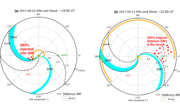
Figure 4: Illustration of the two SIRs detected at Earth (SIR1) and STA (SIR2) as highlighted in Fig. 2. Both SIRs are time shifted to 2017-09-10 at around 19:30 UT shown in (a) and to 2017-09-13 at around 22:00 UT shown in (b). The widths of SIR1 and SIR2 are derived from in-situ their passages at Earth and STA respectively. Norminal IMFs passing Earth, Mars and STA under a solar wind speed of $\sim$ 500 km/s are plotted in dashed lines.

As shown in Fig. 2(i)-(k), SIR2 arrived at STA at about 22:48 UT on 2017-09-13 and the high energy proton flux (up to 100 MeV) has a small enhancement which suggests SEPs may have leaked into, get trapped and/or re-accelerated in the SIR structure. Considering the SIR rotates with the Sun, we time-shift the SIR2 structure observed at STA back to 2017-09-10 at 19:30 UT ($\sim$ shortly before the SEP event at Mars). As illustrated in Fig. 4(a), SIR2 arrived at Mars at almost this time. In fact, in-situ solar wind and magnetic field observations were available during this period and an SIR was identified to have impacted Mars at 23:30 UT (Lee et al., 2018) which perfectly agrees with the time-shifted SIR2 from STA to Mars. Fig. 2(h) also shows the evolution of proton temperature, density and solar wind speed (from $\sim$ 300 to $\sim$ 500 km/s) at Mars during the SIR2 passage which is consistent with the solar wind changes when SIR2 passed STA.

Upon the SEP onset at Mars (Fig. 4(a)), SIR2 was connected even closer to the central part of the shock/flare than Mars. Therefore, SEPs were likely also injected into the SIR structure, preferentially along the IMF direction directly from the shock front as particles cannot easily penetrate through an SIR structure. Such a scenario may have also contributed to the SEPs first arriving at Mars even if Mars were not directly connected to the injection site. These high-energy SEPs were trapped in (or perhaps even re-accelerated therein) and co-rotated with SIR2 and caused a remarkable enhancement of the SEP flux when SIR2 arrived at STA (Fig. 2(i)) at 22:48 UT on 2017-09-13. Since these SEPs were accelerated by the flare/shock closer to the Sun, they have a higher energy component (up to 100 MeV).

On the other hand, SIR1 (cyan area in Fig. 2(a)-(e)) had a more significant enhancement of the solar wind speed (Fig.2(c)) with a more compressed shock structure causing substantial FDs in the NM count rates. It passed Earth starting around 10:15 UT on 2017-09-14. Time-shift analysis shows that shortly after the flare and SEP onset, SIR1 was about 50^∘ west of Earth and was barely magnetically connected to the right edge of the shock as shown in Fig. 4(a), thus making particle injection into SIR1 rather unlikely. It is evident in Fig. 2 (a) that between the shock structure (which passed Earth at 04:00 UT on 2019-09-13, magenta area) and SIR1 arrival at Earth, there is a plateau in the GOES high-energy flux which is different from the declining time profile before the shock arrived at Earth. This may be caused by energetic particles being trapped between the shock and SIR1, which act as two barriers for these SEPs, as illustrated in Fig. 4(b). This is supported by Strauss et al. (2016) who suggested that perpendicular diffusion could be strongly damped at magnetic discontinuities, which may be responsible for the large particle gradients associated with these structures such as an SIR. When SIR1 shock passed Earth, this reservoir of SEPs also passed Earth causing a sudden decrease of the GOES flux at energies below $\sim$ 80 MeV. This decrease is deferent from a normal FD in the GCR flux as seen by NMs on ground.

6 Summary and Conclusion

We investigated and modeled the geometry, kinematics, propagation and interaction of three CMEs launched around 2017-09-10 from their solar origin to their arrivals at Mars and Earth. The modeled results are constrained by and compared with in-situ measurements at Earth, Mars and STA. Observation-based modeling of the ICME and the interplanetary shock reveals the complexity of the event and the advantage of more measurements for advancing space weather predictions. The optimized modeling for the ICME arrival at both Earth and Mars suggests that in order to better predict the ICME arrival and its potential space weather impact at different heliospheric locations, it is important to consider 1) the evolution of the ICME kinematics, especially during interactions of different CMEs and 2) the dynamic heliospheric conditions at different locations in the heliosphere.

The SEP event associated with the flare and the eruption of the last CME has been detected, for the first time, at the surface of two planets, registered as GLE72 at Earth and the biggest GLE seen by MSL/RAD on Mars. Relativistic particles first arriving at Earth and causing GLE72 were mainly accelerated by the flare and the initial shock. The particle onset at Mars is $\sim$ 3.5 hours later than that at Earth and this was caused by either a later magnetic connection of Mars to the shock front which serves as an injection source for SEPs and/or cross-field diffusion of SEPs from the acceleration and injection site. Particles started arriving at STA $\sim$ 1 day16 hours later with a gradual rising profile indicating perpendicular diffusion across IMF was mostly responsible at this phase. Numerical modeling of particle propagation in the heliosphere taking into account of the dynamic acceleration and injection process would also be helpful for understanding the interplanetary journey of these highly energetic particles arriving at three locations $>$ 230^∘ longitudinally apart.

Two SIRs have been detected in-situ at Earth and STA respectively. We shifted SIR2 (detected at STA) back in time and found that its arrival time at Mars is coincident with the SEP onset time at Mars and it had a magnetic connection even closer to the central part of the shock. This may have favored particles injected into the SIR which were later observed as an enhancement in the SEP flux when it passed STA. On the other hand, SIR1 arrived at Earth $\sim$ 1.5 days after the CME shock passed Earth and SEPs were trapped between these two structures causing a plateau profile in the GOES SEP flux.

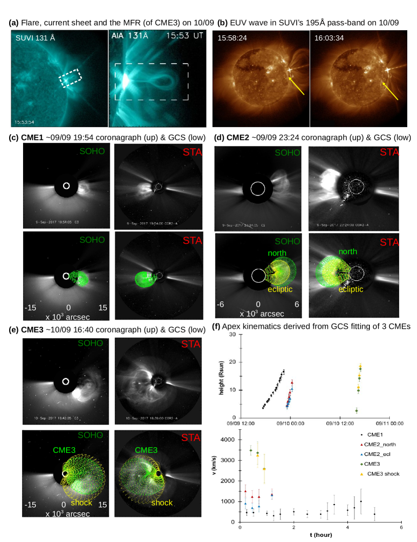
Figure 1: Remote sensing observations of the 2017-09-10 flare and three CMEs launched in the same AR from 2017-09-09 to 2017-09-10. (a) shows the GOES/SUVI 131 Å (adapted from Seaton and Darnel (2018)) and SDO/AIA 131 Å (adapted from Li et al. (2018)) observations of the flare and initial eruption of the MFR (associated with CME3) with the white dashed box marking the flare, current sheet and MFR. (b) displays the post-eruption phase of the MFR and fast propagation of the EUV wave away from the onset location with the yellow arrow pointing at the wave front. (c)-(e) (top panels) show stereoscopic coronagraph WL images (equal ranges in x and y axes) of CME1, CME2 and CME3 at selected times. The bottom panels illustrate GCS reconstruction of the CME geometry. The northern and ecliptic components of CME2 have been fitted respectively and the CME and shock components of CME3 have also been modeled separately. (f) plots apex kinematics derived from GCS modeling of each CME evolution in time. The upper panel shows the height (in solar radii) versus time and the lower panel is the velocity-time plot where time is normalized to the the start of each CME.

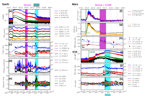
Figure 2: In-situ observations of the 2017-09-10 events at Earth (left panels), Mars (f-h) and STA (i-k). (a)/(i) shows the energy-dependent particle flux (counts/cm²/sr/MeV/sec) measured by GOES and STA. (b) includes count rate of several ground-based neutron monitors with different cut-off rigidities (each neutron monitor data set is normalized to the average value of the selected time range and shifted apart in y-axis). (c) (h) and (j) present the solar wind speed (black, left y-axis (yl)), proton density (blue, right y-axis (yr)) and temperature (red, yr) for Earth (OMNI), Mars (MEX) and STA respectively. The ENLIL modeled results at three locations are also plotted as dashed lines. (d) plots the Alfvén Mach number (black, yl), plasma $\beta$ (blue, yr) and flow pressure (red, yr) estimated at Earth. (e)/(k) displays the vector magnetic fields at Earth/STA in Geocentric Solar Ecliptic (GSE) or spacecraft Radial-Tangential-Normal (RTN) coordinate and negative ENLIL modeled magnetic field strength (dashed line). (f) contains the normalized count rate for downward particles stopping in RAD and penetrating RAD with the former/later approximating protons with energies larger than 175/288 MeV arriving at Mars. (g) shows the dose rate recorded in RAD B (silicon) and E (plastic) detectors. Magenta highlighted areas are the ICME and/or its associated shock passage at Earth and Mars. Cyan highlighted areas are high-speed streams (of two different ones) passing Earth and STA during this period. Vertical solid lines in (a)-(b)/(f)-(g)/(i) indicate the particle onset time at Earth/Mars/STA.

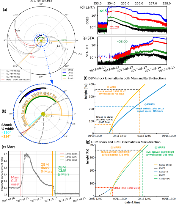
Figure 3: (a) shows heliospheric locations of the Earth, Mars and STA in HEE coordinates. Longitudinal extents of 3 CMES and the interplanetary shock driven by CME3 are approximated by circular contours (their geometries are not modeled as sun-centered circles). Norminal IMFs passing three observers under different solar wind conditions are plotted. At $\sim$ 19:30 the shock (yellow countour) is at a distance of 47 $R_{s}$. Yellow cone boundaries show the extent of the shock with a half-width of 114^∘ which could connect to the 500km/s solar wind IMF towards Mars upon the SEP onset. (b) is a zoom-in of (a) within 0.3 AU and also shows the left edge of the shock with a half-width of 110^∘ not connecting to the 500km/s Parker spiral. (c) plots the enhancement rate (to the background value) representing SEPs $\geq$ about 275 MeV reaching Mars. (d) and (e) show the energy-dependent particle flux measured by GOES at Earth and STA (units and legends are the same as in Fig.2). (f) and (g) are the best-fitting DBM results of the shock and ICME kinematics in Mars and Earth directions with more descriptions and discussions in Section 2-4.

Appendix A References of the measurements and databases employed in this study

In this appendix, we provide descriptions and references of all the data from various spacecraft, instruments and databases employed in this study.

1. High energetic proton data from the Energetic Proton Electron and Alpha Detector (EPEAD) of the Geostationary Operational Environmental Satellite system 15 (GOES15) have been plotted in Fig. 2(a) and Fig. 3(d). The data are documented at www.ngdc.noaa.gov/stp/satellite/goes/ and are publicly available at https://satdat.ngdc.noaa.gov/.

2. Earth ground-based Neutron Monitors (NMs) measure the secondary particles generated in the atmosphere by primary cosmic energetic charged particles including galactic cosmic rays (GCRs) and solar energetic particles (SEPs). The NM data plotted in Fig. 2(b) are obtained from the Neutron Monitor Data Base (NMDB, www.nmdb.eu/nest/).

3. The Space Physics Data Facility (SPDF) OMNIWeb database (https://omniweb.gsfc.nasa.gov/) provides the solar wind data combined from different measurements of available spacecraft including the Advanced Composition Explorer (ACE, Stone et al., 1998), WIND (Lin et al., 1995) and the International Monitoring Platform (IMP)-8. Data plotted in Fig. 2(c)-(e) are in 5 min resolution and the magnetic fields are in the Geocentric Solar Ecliptic (GSE) coordinate.

4. The Radiation Assessment Detector (RAD, Hassler et al., 2012) measures GCRs and SEPs and their secondaries generated in the Martian atmosphere and regolith at Gale Crater on the surface of Mars since the landing of the Curiosity rover in August 2012. Fig. 2(f) plots the normalized (data divided by the background value) RAD level 2 count rate with the blue curve for particles stopping inside the detector and red curve for particles penetrating through the whole instruments. The average vertical column depth of the atmosphere on top of RAD was about 23.4 g/cm² during the period of the event. This would only allow protons with kinetic energies larger than about 175 MeV to reach the surface (Guo et al., 2018b) which translates into the minimum primary energy for protons (SEP on top of the atmosphere) stopping in RAD. For protons to penetrate through the entire detector stack, a minimum energy of 113 MeV is required and this adds to about 288 MeV of primary SEP energy. Note that this approximation is under the assumption that the majority of particles reaching Mars surface are protons which is valid during the SEP events. Fig. 2(g) plots the RAD dose rate [mGray/day] recorded in B (silicon) and E (plastic) detectors. Dose rate is a measure of the energy [$10^{-3}$ Joule] deposited by all detected particles per detector mass [kg] per time unit [day]. A zoomed-in plot (to emphasize the onset of the SEP) of the enhancement ratio of the dose rate (normalized to the background value) in the plastic detector is shown in Fig. 3(c). For downward directed particles during the solar event, they need $\sim$ 100 MeV kinetic energy to reach the E detector. This corresponds to a primary SEP energy $\geq$ about 275 MeV arriving at Mars. Both the count rate and dose rate data are generally in cadence of 17 minutes as RAD runs on an autonomous observing cycle with 16 minutes per observation plus 1 minute of sleep mode.

5. The Analyzer of Space Plasmas and EneRgetic Atoms (ASPERA-3, Barabash et al., 2006) experiment of the Mars-EXpress (MEX) mission has been used to derive the solar wind properties (Ramstad et al., 2015) plotted in Fig. 2(h), including the proton density, temperature and solar wind speed.

6. The High Energy Telescope (HET, Von Rosenvinge et al., 2008) on the Solar Terrestrial relations observatory Ahead (STA) spacecraft provides proton flux rate in various energy ranges which are combined into 4 different channels and plotted in Fig. 2(i). The STA Plasma and Suprathermal Ion Composition (PLASTIC, Galvin et al., 2008) measurement of the solar wind properties (proton density, temperature and solar wind speed) is shown in Fig. 2(j). The In situ Measurements of Particles And CME Transients (IMPACT) data of the magnetic field experiment (Acuña et al., 2008) on STA are plotted in Fig. 2(k) in the spacecraft Radial-Tangential-Normal (RTN) coordinate.

7. Remote-sensing coronagraph images of the Sun at two different heliospheric locations have been obtained from a) the Large Angle and Spectrometric Coronagraph (LASCO, Brueckner et al., 1995) instrument onboard the Solar and Heliospheric Observatory (SOHO) at Earth and b) the coronagraph (COR) data from the Sun Earth Connection Coronal and Heliospheric Investigation (SECCHI, Howard et al., 2008) at STA.

8. Observations of extreme-ultraviolet (EUV) phenomena in the solar corona are shown in Fig. 1(a) and (b). They are from the Solar Ultraviolet Imager (SUVI) on the GOES16 spacecraft and the Atmospheric Imaging Assembly (AIA, Lemen et al., 2011) on board the Solar Dynamics Observatory (SDO) spacecraft.