Abstract

The Brio system is a two-by-two system of conservation laws arising as a simplified model in ideal magnetohydrodynamics (MHD). The system has the form

$$\partial_{t}u+\partial_{x}\big{(}{\textstyle\frac{u^{2}+v^{2}}{2}}\big{)}=0,$$

$$\partial_{t}v+\partial_{x}\big{(}v(u-1)\big{)}=0.$$

It was found in previous works that the standard theory of hyperbolic conservation laws does not apply to this system since the characteristic fields are not genuinely nonlinear on the set $v=0$. As a consequence, certain Riemann problems have no weak solutions in the traditional class of functions of bounded variation.

It was argued in [8] that in order to solve the system, singular solutions containing Dirac masses along the shock waves might have to be used. Solutions of this type were exhibited in [11, 23], but uniqueness was not obtained.

In the current work, we introduce a nonlinear change of variables which makes it possible to solve the Riemann problem in the framework of the standard theory of conservation laws. In addition, we develop a criterion which leads to an admissibility condition for singular solutions of the original system, and it can be shown that admissible solutions are unique in the framework developed here.

1 Introduction

Conservation laws have been used as a mathematical tool in a variety of situations in order to provide a simplified description of complex physical phenomena which nevertheless keeps the essential features of the processes to be described, and the general theory of hyperbolic conservation laws aims to provide a unified set of techniques needed to understand the mathematical properties of such equations. However, in some cases, the general theory fails to provide a firm mathematical description for a particular case because some of the assumptions needed in the theory are not in place.

In the present contribution we focus on such an example, a hyperbolic conservation law appearing in ideal magnetohydrodynamics. For this conservation law, solutions cannot be found using the classical techniques of conservation laws, and a new approach is needed.

Magnetohydrodynamics (MHD) is the study of how electric currents in a moving conductive fluid interact with the magnetic field created by the moving fluid itself. The MHD equations are a combination of the Navier-Stokes equations of fluid mechanics and Maxwell’s equations of electromagnetism, and the equations are generally coupled in such a way that they must be solved simultaneously. The ideal MHD equations are based on a combination of the Euler equations of fluid mechanics (i.e. for an inviscid and incompressible fluid) and a simplified form of Maxwell’s equations. The resulting system is highly complex and one needs to rely on numerical approximation of solutions in order to understand the dynamics of the system.

As even the numerical study of the full system is very challenging, it can be convenient to introduce some simplifying assumptions – valid in some limiting cases – in order to get a better idea of the qualitative properties of the system, and in order to provide some test cases against which numerical codes for the full MHD system can be tested.

The emergence of coherent structures in turbulent plasmas has been long observed both in numerical simulations and experiments. Moreover, the tendency of the magnetic field to organize into low-dimensional structures such as two-dimensional magnetic pancakes and one-dimensional magnetic ropes is well known. As a consequence, in certain cases it makes sense to use simplified one or two dimensional model equations. Such simplified equations will be easier to solve, but nevertheless preserve some of the important features observed in MHD systems. In [1], a simplified model system for ideal MHD was built using such phenomenological considerations. The system is written as

$$\begin{split}\partial_{t}u+\partial_{x}\big{(}{\textstyle\frac{u^{2}+v^{2}}{2}}\big{)}=0,\\ \partial_{t}v+\partial_{x}\big{(}v(u-1)\big{)}=0.\end{split}$$ (1)

The quantities $u$ and $v$ are the velocity components of the fluid whose dynamics is determined by MHD forces, and the system represents the conservation of the velocities. Velocity conservation in this form holds only in idealized situations in the case of smooth solutions, and the limitation of this assumption manifests itself in the non-solvability of the system even for the simplest piece-wise constant initial data, i.e. for certain dispositions of the Riemann initial data

$$u|_{t=0}=\begin{cases}U_{L},&x\leq 0\\ U_{R},&x>0\end{cases},\qquad v|_{t=0}=\begin{cases}V_{L},&x\leq 0\\ V_{R},&x>0\end{cases}.$$ (2)

From a mathematical point of view, the characteristic fields of this system are neither genuinely nonlinear nor linearly degenerate in certain regions in the $(u,v)$-plane (see [8]). In this case the standard theory of hyperbolic conservation laws which can be found in e.g. [3] does not apply and one cannot find a classical Riemann solution admissible in the sense of Lax [17] or Liu [18].

In order to deal with the problem of non-existence of solutions to the Riemann problem for certain conservation laws, the concept of singular solutions incorporating $\delta$-distributions along shock trajectories was introduced in [16]. The idea was pursued further in [15, 8], and by now, the literature on the subject is rather extensive. Some authors have defined theories of distribution products in order to incorporate the $\delta$-distributions into the notion of weak solutions [4, 10, 23]. In other works, the need to multiply $\delta$-distributions has been avoided either by working with integrated equations [9, 13], or by making an appropriate definition of singular solutions [6]. In order to find admissibility conditions for such singular solutions, some authors have used the weak asymptotic method [6, 5, 21, 22]. With the aim of dealing with the nonlinearity featured by the system (1), the weak asymptotic method was also extended to include complex-valued approximations [11]. The authors of [11] were able to provide singular solutions of (1) even in cases which could not be resolved earlier. However, even if [11] provides some admissibility conditions, the authors of [11] did not succeed to prove uniqueness. Existence of singular solutions to (1) was also proved in [23] using the theory of distribution products, but uniqueness could not be obtained.

Therefore, it was natural to ask whether the Brio system should be solved in the framework of $\delta$-distributions as conjectured in [8] where the system was first considered from the viewpoint of the conservation laws theory. The authors of [8] compared (1) with the triangular system

$$\begin{split}\partial_{t}u+\partial_{x}\big{(}{\textstyle\frac{u^{2}}{2}}\big{)}=0,\\ \partial_{t}v+\partial_{x}\big{(}v(u-1)\big{)}=0.\end{split}$$ (3)

which differs from (1) in the quadratic term $v^{2}$. However, the system (3) is linear with respect to $v$ and it naturally admits $\delta$-type solutions (obtained e.g. via the vanishing viscosity approximation). To this end, let us remark that most of the systems admitting $\delta$-shock wave solutions are linear with respect to one of the unknown functions [4, 6, 8, 10, 15]. There are also a number of systems which can be solved only by introducing the $\delta$-solution concept and which are non-linear with respect to both of the variables such as the chromatography system [24] or the Chaplygin gas system [20]. However, in all such systems, it was possible to control the nonlinear operation over an approximation of the $\delta$-distribution. This is not the case with (1) since the term $u^{2}+v^{2}$ will necessarily tend to infinity for any real approximation of the $\delta$-function. This problem can be dealt with by introducing complex-valued approximations of the $\delta$-distribution. Using this approach, a somewhat general theory can be developed as follows. Consider the system

$$\begin{split}\partial_{t}u+\partial_{x}f(u,v)=&0,\\ \partial_{t}v+\partial_{x}g(u,v)=&0,\end{split}$$ (4)

The following definition gives the notion of $\delta$-shock solution to system (4).

Definition 1.1.

The pair of distributions

$$u=U+\alpha(x,t)\delta(\Gamma)\ \ \text{and}\ \ v=V+\beta(x,t)\delta(\Gamma)$$ (5)

are called a generalized $\delta$-shock wave solution of system (4) with the initial data $U_{0}(x)$ and $V_{0}(x)$ if the integral identities

$$\int_{I\!\!R_{+}}\!\!\int_{I\!\!R}\left(U\partial_{t}\varphi+f(U,V)\partial_{x}\varphi\right)~{}dxdt$$

$$\qquad+\sum\limits_{i\in I}\int_{\gamma_{i}}\alpha_{i}(x,t){\textstyle\frac{\partial\varphi(x,t)}{\partial{\bf l}}}\,+\int_{I\!\!R}U_{0}(x)\varphi(x,0)~{}dx=0,$$ (6)

$$\int_{I\!\!R_{+}}\!\!\int_{I\!\!R}\left(V\partial_{t}\varphi+g(U,V)\partial_{x}\varphi\right)~{}dxdt$$

$$\qquad+\sum\limits_{i\in I}\int_{\gamma_{i}}\beta_{i}(x,t){\textstyle\frac{\partial\varphi(x,t)}{\partial{\bf l}}}\,+\int_{I\!\!R}V_{0}(x)\varphi(x,0)~{}dx=0,$$ (7)

hold for all test functions $\varphi\in{\mathcal{D}}(I\!\!R\times I\!\!R_{+})$.

This definition may be interpreted as an extension of the classical notion of weak solutions. The definition is consistent with the concept of measure solutions as put forward in [4, 10] in the sense that the two singular parts of the solution coincide, while the regular parts differ on a set of Lebesgue measure zero. However, Definition 1.1 can be applied to any hyperbolic system of equations while the solution concept from [4] only works in the special situation when the $\delta$-distribution is attached to an unknown which appears linearly in the flux $f$ or $g$, or when nonlinear operations on $\delta$ can somehow be controlled in another way.

Definition 1.1 is quite general, allowing a combination of initial steps and delta distributions; but its effectiveness is already demonstrated by considering the Riemann problem with a single jump. Indeed, for this configuration it can be shown that a $\delta$-shock wave solution exists for any $2\times 2$ system of conservation laws.

Consider the Riemann problem for (4) with initial data $u(x,0)=U_{0}(x)$ and $v(x,0)=V_{0}(x)$, where

$$U_{0}(x)=\begin{cases}u_{1},&x<0,\\ u_{2},&x>0,\end{cases}\quad V_{0}(x)=\begin{cases}v_{1},&x<0,\\ v_{2},&x>0.\end{cases}$$ (8)

Then, the following theorem holds:

Theorem 1.2.

a) If $u_{1}\neq u_{2}$ then the pair of distributions

$$u(x,t) = U_{0}(x-ct),$$ (9)

$$v(x,t) = V_{0}(x-ct)+\beta(t)\delta(x-ct),$$ (10)

where

$$c=\frac{[f(U,V)]}{[U]}=\frac{f(u_{2},v_{2})-f(u_{1},v_{1})}{u_{2}-u_{1}},\ \mbox{ and }\ \beta(t)=(c[V]-[g(U,V)])t,$$ (11)

represents the $\delta$-shock wave solution of (4) with initial data $U_{0}(x)$ and $V_{0}(x)$ in the sense of Definition 1.1 with $\alpha(t)=0$.

b) If $v_{1}\neq v_{2}$ then the pair of distributions

$$u(x,t) = U_{0}(x-ct)+\alpha(t)\delta(x-ct),$$ (12)

$$v(x,t) = V_{0}(x-ct),$$ (13)

where

$$c=\frac{[g(U,V)]}{[V]}=\frac{g(u_{2},v_{2})-g(u_{1},v_{1})}{v_{2}-v_{1}},\ \ \alpha(t)=(c[U]-[f(U,V)])t$$ (14)

represents the $\delta$-shock solution of (4) with initial data $U_{0}(x)$ and $V_{0}(x)$ in the sense of Definition 1.1 with $\beta(t)=0$.

Proof.

We will prove only the first part of the theorem as the second part can be proved analogously. We immediately see that $u$ and $v$ given by (9) and (10) satisfy (1.1) since $c$ is given exactly by the Rankine-Hugoniot condition derived from that system. By substituting $u$ and $v$ into (1.1), we get after standard transformations:

$$\int_{I\!\!R_{+}}\left(-c[V]+[g(u,V)]\right)\varphi(ct,t)~{}dt-\int_{I\!\!R_{+}}\alpha^{\prime}(t)\varphi(ct,t)~{}dt=0.$$

From here and since $\alpha(0)=0$, the conclusion follows immediately. ∎

As the solution framework of Definition 1.1 is very weak, one might expect non-uniqueness issues to arise. This is indeed the case, and the proof of the following proposition is an easy exercise.

Proposition 1.3.

System (4) with the zero initial data: $u|_{t=0}=v|_{t=0}=0$ admits $\delta$-shock solutions of the form:

$$u(x,t)=0,\ \ v(x,t)=\beta\delta(x-c_{1}t)-\beta\delta(x-c_{2}t),$$

for arbitrary constants $\beta$, $c_{1}$ and $c_{2}$.

As already alluded to, a different formal approach for solving (1) was used by [23]. However, just as in [11] the definition of singular solutions used in [23] is so weak that uniqueness cannot be obtained. Another problem left open in [11, 23] is the physical meaning of the $\delta$-distribution appearing as the part of the solution. Considering systems such as the Chaplygin gas system or (3), the use of the $\delta$-distribution in the solution can be justified by invoking extreme concentration effects if we assume that $v$ represents density. However, in the case of the Brio system, $u$ and $v$ are velocities and unbounded velocities cannot be explained in any reasonable physical way.

In the present contribution, we shall try to explain necessity of $\delta$-type solutions for (1) following considerations from [14] where it was argued (in a quite different setting) that the wrong variables are conserved. In other words, the presence of a $\delta$-distribution in a weak solution actually signifies the inadequacy of the corresponding conservation law in the case of weak solutions. Similar consideration were recently put forward in the case of singular solutions in the shallow-water system [12].

Starting from this point, we are able to formulate uniqueness requirement for the Riemann problem for (1). First, we shall rewrite the system using the energy $q=(u^{2}+v^{2})/2$ as one of the conserved quantities (which is actually an entropy function corresponding to (1)). Thus, we obtain a strictly hyperbolic and genuinely nonlinear system which admits a Lax admissible solution for any Riemann problem. Such a solution is unique and it will give a unique $\delta$-type solution to the original system. The $\delta$-distribution will necessarily appear due to the nonlinear transformation that we apply.

The paper is organized as follows: In Section 2, we shall rewrite (1) in the new variables $q$ and $u$, and exhibit the admissible shock and rarefaction waves. In Section 3, we shall introduce the admissibility concept for solutions of the original system (1), and prove existence and uniqueness of a solution to the Riemann problem in the framework of that definition.

2 Energy-velocity conservation

As mentioned above, conservation of velocity is not necessarily a physically well defined balance law, and it might be preferable to specify conservation of energy for example. Actually, in some cases, conservation of velocity does give an appropriate balance law, such as for example in the case of shallow-water flows [7]. In the present situation, it appears natural to replace at least one of the equations of velocity conservation. As will be seen momentarily, such a system will be strictly hyperbolic with genuinely nonlinear characteristic fields, so that the system will be more amenable to standard method of hyperbolic conservation laws. To introduce the new conservation law, we define an energy function

$$q(u,v)=\frac{u^{2}+v^{2}}{2},$$ (15)

and note that this function is a mathematical entropy for the system (1). Then we use the transformation

$$(u,v)\rightarrow\big{(}u,{\textstyle\frac{u^{2}+v^{2}}{2}}\big{)},$$

to transform (1) into the system

$$\begin{split}\partial_{t}u+\partial_{x}q=0,\\ \partial_{t}q+\partial_{x}\big{(}(2u-1)q+{\textstyle\frac{u^{2}}{2}}-{\textstyle\frac{2u^{3}}{3}}\big{)}=0.\end{split}$$ (16)

System (1) and the transformed system (16) are equivalent for differentiable solutions. However, as will be evident momentarily, the nonlinear transformation changes the character of the system, and while (1) is not always genuinely nonlinear, the new system (16) is always strictly hyperbolic and genuinely nonlinear.

In the following, we analyze (16), and find the elementary waves for the solution of (16). The flux function of the new system is given by

$$F=\begin{pmatrix}q\\ (2u-1)q+\frac{u^{2}}{2}-\frac{2u^{3}}{3}\end{pmatrix}$$

with flux Jacobian

$$DF=\begin{pmatrix}0&1\\ 2q+u-2u^{2}&2u-1\end{pmatrix}.$$

The characteristic velocities are given by

$$\lambda_{-,+}=\frac{2u-1\mp\sqrt{8q-4u^{2}+1}}{2}.$$ (17)

A direct consequence of (15) gives the relation $2q\geq u^{2}\geq 0$ which implies that the quantity under the square root is non-negative. Thus, $8q-4u^{2}+1>0$ and the eigenvalues are real and distinct so that the system is strictly hyperbolic. The right eigenvectors in this case are given by

$$\begin{split}r_{-}=\begin{pmatrix}1\\ u-\frac{1}{2}-\sqrt{2q-u^{2}+\frac{1}{4}}\end{pmatrix},\\ r_{+}=\begin{pmatrix}1\\ u-\frac{1}{2}+\sqrt{2q-u^{2}+\frac{1}{4}}\end{pmatrix}.\end{split}$$ (18)

It can be verified easily that these eigenvectors are linearly independent and span the $(u,q)$-plane. The associated characteristic fields

$$\nabla\lambda_{-}\cdot r_{-}=2+\frac{1}{\sqrt{8q-4u^{2}+1}}\ ,$$ (19)

$$\nabla\lambda_{+}\cdot r_{+}=2-\frac{1}{\sqrt{8q-4u^{2}+1}}\ ,$$ (20)

are genuinely nonlinear and admit both shock and rarefaction waves. For a shock profile connecting a constant left state $(u,q)=(u_{L},q_{L})$ to a constant right state $(u,q)=(u_{R},q_{R})$, the Rankine-Hugoniot jump conditions for (16) are

$$c(u_{L}-u_{R}) =~{}(q_{L}-q_{R}),$$ (21)

$$c(q_{L}-q_{R}) =\big{(}(2u_{L}-1)q_{L}+{\textstyle\frac{u_{L}^{2}}{2}}-{\textstyle\frac{2u_{L}^{3}}{3}}-(2u_{R}-1)q_{R}-{\textstyle\frac{u_{R}^{2}}{2}}+{\textstyle\frac{2u_{R}^{3}}{3}}\big{)},$$ (22)

where $c$ is the shock speed. We want the speed in (21), (22) to satisfy the Lax admissibility condition

$$\lambda_{\mp}(u_{L},q_{L})\geq c\geq\lambda_{\mp}(u_{R},q_{R}).$$ (23)

To determine the set of all states that can be connected to a fixed left state $(u_{L},q_{l})$, we eliminate the shock speed, $c$, from the above equations to obtain the shock curves

$$(q_{R})_{1,2}=\frac{2q_{L}-(u_{L}-u_{R})(2u_{R}-1)}{2}\ \ \pm\ \ \ \ \ \ \ \ \ \ \ \ \ \ \ \ \ \ \ \ \ \ \ \ \ \ \ \ \ \ \ \ \ \ \ \ \ \ \ \ \ \ \ \ \ \ \ \ \ \$$

$$\frac{\sqrt{[-2q_{L}+(u_{L}-u_{R})(2u_{R}-1)]^{2}+4\left[(u_{L}-u_{R})\left((2u_{L}-1)q_{L}+\frac{u_{L}^{2}}{2}-\frac{u_{R}^{2}}{2}-\frac{2u_{L}^{3}}{3}+\frac{2u_{R}^{3}}{3}\right)-q_{L}^{2}\right]}}{2}.$$

After basic algebraic manipulations, we obtain

$$(q_{R})_{1,2}=q_{L} -\frac{1}{2}(u_{L}-u_{R})(2u_{R}-1)$$

$$\pm\mid u_{L}-u_{R}\mid\sqrt{2q_{L}+{\textstyle\frac{1}{4}}+{\textstyle\frac{1}{2}}(u_{L}-u_{R})-{\textstyle\frac{1}{3}}\big{(}2u_{L}^{2}+2u_{L}u_{R}-u_{R}^{2}\big{)}}$$ (24)

From here and (23), by considering $(u_{R},q_{R})$ in a small neighborhood of $(u_{L},q_{L})$, we conclude that the shock wave of the first family (SW1), the shock wave of the second family (SW2), the rarefaction wave of the first family (RW1) and the rarefaction wave of the second family (RW2) are given as follows:

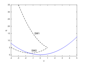
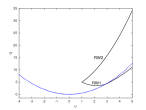
(a)                                                        (b)

Figure 1: (a) Shock wave curves of the first and the second families at the left state $(u_{L},q_{L})=(1,5)$. (SW1) is indicated by the upper curve, while (SW2) is the lower curve. The blue dotted curve shows the limiting curve $q=u^{2}/2$. (b) Rarefaction wave curves of the first and the second families at the left state $(u_{L},q_{L})=(1,5)$. The (RW1) is indicated by the lower curve while (RW2) is the upper curve.

$$\mathrm{(SW1)}\ \ q_{R}=q_{L}-\frac{1}{2}\big{(}u_{L}-u_{R}\big{)}\big{(}2u_{R}-1\big{)}\qquad\qquad\qquad\qquad\qquad\qquad\qquad\qquad\quad\$$

$$+\mid u_{L}-u_{R}\mid\Big{(}2q_{L}+{\textstyle\frac{1}{2}}(u_{L}-u_{R})-{\textstyle\frac{1}{3}}\big{(}2u_{L}^{2}+2u_{L}u_{R}-u_{R}^{2}\big{)}+{\textstyle\frac{1}{4}}\Big{)}^{\frac{1}{2}},\ \$$ (25)

for $u_{R}<u_{L}$. To verify that this indeed is the shock wave of the first family, we obtain from (21) and (23) that

$$\lambda_{-}(u_{L},q_{L})\geq c=\frac{2u_{R}-1-\sqrt{8q_{L}+1+\frac{4u_{R}^{2}}{3}-\frac{8u_{L}u_{R}}{3}-\frac{8u_{L}^{2}}{3}-2u_{R}+2u_{L}}}{2}.$$

Taking into account the form of $\lambda_{-}$, we conclude from the above equation that

$$2(u_{L}-u_{R})\geq\sqrt{8q_{L}+1-4u_{L}^{2}}-\sqrt{8q_{L}+1+\frac{4u_{R}^{2}}{3}-\frac{8u_{L}u_{R}}{3}-\frac{8u_{L}^{2}}{3}-2u_{R}+2u_{L}}.$$

Further simplification leads to

$$2\geq\frac{-\frac{4}{3}(u_{L}-u_{R})-2}{\sqrt{8q_{L}+1-4u_{L}^{2}}+\sqrt{8q_{L}+1+\frac{4u_{R}^{2}}{3}-\frac{8u_{L}u_{R}}{3}-\frac{8u_{L}^{2}}{3}-2u_{R}+2u_{L}}},$$

which is obviously correct. In a similar way, the second part of the Lax condition,

$$\lambda_{-}(u_{R},q_{R})\leq c,$$

can be verified. Moreover, it is trivial to verify the additional inequality $\lambda_{+}(u_{R},q_{R})\geq c$, so that we have three characteristic curves entering the shock trajectory, and one characteristic curve leaving the shock.

$$\mathrm{(SW2)}\ \ q_{R}=q_{L}-\frac{1}{2}\big{(}u_{L}-u_{R}\big{)}\big{(}2u_{R}-1\big{)}\qquad\qquad\qquad\qquad\qquad\qquad\qquad\qquad\quad\$$

$$-\mid u_{L}-u_{R}\mid\Big{(}2q_{L}+{\textstyle\frac{1}{2}}(u_{L}-u_{R})-{\textstyle\frac{1}{3}}\big{(}2u_{L}^{2}+2u_{L}u_{R}-u_{R}^{2}\big{)}+{\textstyle\frac{1}{4}}\Big{)}^{\frac{1}{2}},\ \$$ (26)

for $u_{R}<u_{L}$. We will skip the proof since it is the same as in the case of (SW1). Next, we have the rarefaction curves.

(RW1),  Using the method from [3, Theorem 7.6.5], this wave can be written as

$$\frac{dq}{du}=\frac{2u-1-\sqrt{8q-4u^{2}+1}}{2}=\lambda_{-}(u,q),\ \ \ \ \ q(u_{L})=q_{L},$$ (27)

for $u_{R}>u_{L}$. Clearly, for $u_{R}<u_{L}$ we cannot have (RW1) since in that domain, states are connected by (SW1) (see (SW1) above). In order to prove that (27) indeed provides RW1, we need to show that

$$\lambda_{-}(u_{L},q_{L})<\lambda_{-}(u_{R},q_{R})\ \ {\rm if}\ \ u_{R}>u_{L}.$$ (28)

Introducing the change of variables $\tilde{q}=8q-4u^{2}+1$ in (27), we can rewrite it in the form

$$\frac{d\tilde{q}}{du}=-4(1+\sqrt{\tilde{q}})<0.$$

From here, we see that $\tilde{q}$ is decreasing with respect to $u$ and thus, for $u_{L}<u_{R}$, we must have

$$8q_{L}-4u_{L}^{2}+1=\tilde{q}_{L}>\tilde{q}_{R}=8q_{R}-4u_{R}^{2}+1.$$

This, together with $u_{L}<u_{R}$ immediately implies (28).

(RW2) Using again [3, Theorem 7.6.5]), we have

$$\frac{dq}{du}=\frac{2u-1+\sqrt{8q-4u^{2}+1}}{2}=\lambda_{+}(u,q),\ \ q(u_{L})=q_{L},$$ (29)

for $u_{R}>u_{L}$. It can be shown that (29) gives the rarefaction wave (RW2) in the same way explained above for (RW1). The wave fan issuing from the left state $(u_{L},q_{L})$ and the inverse wave fan issuing from the right state $(u_{R},q_{R})$ are given in Figure 2(a) and Figure 2(b), respectively.

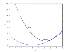
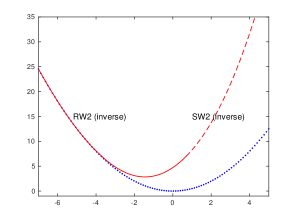
(a)                                                        (b)

Figure 2: Shock and rarefaction wave curves of the first and the second families: (a) shows SW1 (dashed) and RW1 (solid) at the left state $(u_{L},q_{L})=(1,5)$. (b) shows inverse SW2 (dashed, red) and inverse RW2 (solid, red) at the right state $(u_{R},q_{R})=(0.7,7)$.

We next aim to prove existence of solution for arbitrary Riemann initial data without necessarily assuming a small enough initial jump. The only essential hypothesis is that both left and right states are above the critical curve $q_{crit}=u^{2}/2$:

$$q_{L}\geq u_{L}^{2}/2,\ \ \ \ q_{R}\geq u_{R}^{2}/2.$$ (30)

This assumptions is of course natural given the change of variables $q=\frac{u^{2}+v^{2}}{2}$. Nevertheless, this condition makes complicates our task since is also needs to be shown that the Lax admissible solution to a Riemann problem remains in the area $q\geq u^{2}/2$. To this end, the following lemma will be useful.

Lemma 2.1.

The function $q_{crit}(u)=\frac{u^{2}}{2}$ satisfies (29).

Proof.

The proof is obvious and we omit it. ∎

The above lemma is important since, according to the uniqueness of solutions to the Cauchy problem for ordinary differential equations, it shows that if the left and right states $(u_{L},q_{L})$ and $(u_{R},q_{R})$ are above the curve $q_{crit}(u)=\frac{u^{2}}{2}$, then the simple waves (SW1, SW2, RW1, RW2) connecting the states will remain above it which means that we can use the solution to (16) to obtain a solutions of (1) since the square root giving the function $v=\sqrt{2q-u^{2}}$ will be well defined. Concerning the Riemann problem, we have the following theorem.

Theorem 2.2.

Given a left state $(u_{L},q_{L})$ and a right state $(u_{R},q_{R})$, so that both are above the critical curve $q_{crit}(u)=\frac{u^{2}}{2}$ i.e. we have $q_{L}\geq u_{L}^{2}/2$ and $q_{R}\geq u_{R}^{2}/2$, the states $(u_{L},q_{L})$ and $(u_{R},q_{R})$ can be connected Lax admissible shocks and rarefaction waves via a middle state belonging to the domain $q>u^{2}/2$.

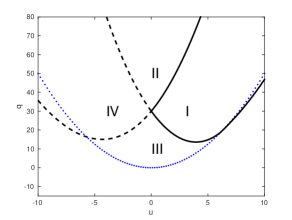
Figure 3: Admissible connections between a given left state $(u_{L},q_{L})$ and a right state can be classified into four regions in the phase plane.

Proof.

In order to find a connection between $(u_{L},q_{L})$ and $(u_{R},q_{R})$, we first draw the waves of the first family (SW1 and RW1) through $(u_{L},q_{L})$ and waves of the second family (SW2 and RW2) through $(u_{R},q_{R})$. The point of intersection will be the middle state through which we connect $(u_{L},q_{L})$ and $(u_{R},q_{R})$ (see Figure 4 for different dispositions of $(u_{L},q_{L})$ and $(u_{R},q_{R})$). In this case, the intersection point will be unique which can be seen by considering the four possible dispositions of the states $(u_{L},q_{L})$ and $(u_{R},q_{R})$ shown in Figure 4:

• For right states in region $I$: RW1 followed by RW2;

• For right states in region $II$: SW1 followed by RW2;

• For right states in region $III$: RW1 followed by SW2;

• For right states in region $IV$: SW1 followed by SW2;

Properties of the curves of the first and second families are provided in a)-d) above. The growth properties give also existence as we shall show in detail in the sequel of the proof.

Firstly, we remark that SW1 and RW1 emanating from $(u_{L},q_{L})$ cover the entire $q\geq u^{2}/2$ domain (see Figure 2(a)). In other words, we have for the curve $q_{R}$ defining the SW1 by (2):

$$\lim\limits_{u_{R}\to-\infty}q(u_{R})=\infty,$$

implying that the SW1 will take all $q$-values for $q_{R}>q_{L}$. More precisely, for every $q_{R}>q_{L}$ there exists $u_{R}<u_{L}$ such that $q_{R}(u_{R})=q_{R}$ where $q_{R}$ is given by (2).

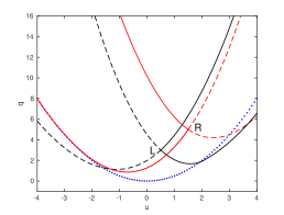
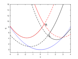
(a)                                                        (b)   

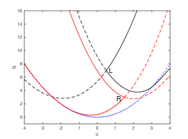
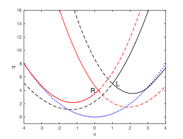
(c)                                                        (d)

Figure 4: Shock and rarefaction wave curves of the first and the second families. At the left state $L=(u_{L},q_{L})$, the curves SW1 (dashed), SW2 (dashed), RW1 (solid), and RW2 (solid) are drawn in black. The inverse curves at the right state $R=(u_{R},q_{R})$ are indicated in red: SW1 (dashed), SW2 (dashed), RW1 (solid) and RW2 (solid). Panel (a) shows the situation for region I, Panel (b) shows the situation for region II, Panel (c) shows the situation for region III and Panel (d) shows the situation for region IV.

As for the RW1, it holds for $q$ given by (27) that

$$\frac{dq}{du}-u\leq-1\implies\frac{dq}{du}\leq u-1,$$

which means that the RW1 curve emanating from any $(u_{L},q_{L})$ for which $q_{L}>u_{L}^{2}/2$ will intersect the curve $q_{crit}=\frac{u^{2}}{2}$ (since $\frac{dq_{crit}}{du}=u>u-1\geq\frac{dq}{du}$) at some $u_{R}>u_{L}$ as shown in Figure 1, b).

Now, we turn to the waves of the second family. Let us fix the right state $(u_{R},q_{R})$. We need to compute the inverse waves (i.e. for the given right state, we need to compute curves consisting of appropriate left states (see Figure 2(b)). The inverse rarefaction curve of the second family is given by the equation (29), but we need to take values for $u_{R}<u_{L}$ (opposite to the ones given in (29)). As for the inverse SW2, we compute from (21) and (22) the value $q_{L}$:

$$q_{L}=q_{R} -\frac{1}{2}\big{(}u_{L}-u_{R}\big{)}\big{(}2u_{L}-1\big{)}$$

$$+\frac{(u_{L}-u_{R})}{2}\sqrt{8q_{R}+1+{\textstyle\frac{4u_{L}^{2}}{3}}-{\textstyle\frac{8u_{L}u_{R}}{3}}-{\textstyle\frac{8u_{R}^{2}}{3}}-2u_{L}+2u_{R}},$$ (31)

for $u_{R}<u_{L}$. Clearly, the RW2 cannot intersect the critical line $q_{crit}=\frac{u^{2}}{2}$ since $q_{crit}$ satisfy (29) (see Lemma 2.1) and the intersection would contradict uniqueness of solution to the Cauchy problem for (29). However, a solution to (29) with the initial conditions $q(u_{R})=q_{R}>u_{R}^{2}/2$ will converge toward the line $q_{crit}=u^{2}/2$ since for $q$ given by (29) we have

$$\frac{dq}{du}-u\geq 0\ \ {\rm and}\ \ \frac{dq}{du}\Big{|}_{(u,u^{2}/2)}-u=0,$$

implying that $q$ will decrease toward $q_{crit}=u^{2}/2$ and that they will merge as $u_{L}\to-\infty$ (see Figure 2(b)). As for the inverse SW2 given by (2), we see that

$$\lim\limits_{u_{L}\to\infty}q(u_{L})=\infty,$$

which eventually imply that the 1-wave family emanating from $(u_{L},q_{L})$ must intersect with the inverse 2-wave family emanating from $(u_{R},q_{R})$ somewhere in the domain $q>u^{2}/2$ (see Figure 4 for several dispositions of the left and right states).

Finally, we remark that according to the previous analysis, it follows that the intersection between curves of the first and the second family is unique. ∎

3 Admissibility conditions for $\delta$-shock wave solution to the original Brio System

Our starting point is that the system original Brio system (1) is based on conservation of quantities which are not necessarily physically conserved, and that the transformed system (16) is a closer representation of the physical phenomenon to be described. The second principle is that $\delta$-distribution represents actually a defect in the model and thus, it should be necessarily present as a part of non-regular solutions to (1). Moreover, the regular part of a solution to (1) should be an admissible solution to (16). Having these requirements in mind, we are able to introduce admissibility conditions for a $\delta$-type solution to (1).

Let us first recall the characteristic speeds for (1). Following the [8], we see immediately that

$$\lambda_{1}(u,v)=u-1/2-\sqrt{v^{2}+1/4},\ \ \lambda_{2}(u,v)=u-1/2+\sqrt{v^{2}+1/4}.$$ (32)

The shock speed for (1) for the shock determined by the left state $(U_{L},V_{L})$ and the right state $(U_{R},V_{R})$ is given by

$$s=\frac{U_{L}+U_{R}}{2}+\frac{V_{L}^{2}-V_{R}^{2}}{2(U_{L}-U_{R})}.$$ (33)

Now, we can formulate admissibility conditions for $\delta$-type solution to (1) in the sense of Definition 1.1. We shall require that the real part of $\delta$-type solution to (1) satisfy the energy-velocity conservation system (16) and that the number of $\delta$-distributions appearing as part of the solution to (1) is minimal.

Definition 3.1.

We say that the pair of distributions $u=U+\alpha(x,t)\delta(\Gamma)$ and $v=V+\beta(x,t)\delta(\Gamma)$ satisfying Definition 1.1 with $f(u,v)=\frac{u^{2}+v^{2}}{2}$ and $g(u,v)=v(u-1)$ is an admissible $\delta$-type solution to (1), (2) if

• The regular parts of the distributions $u$ and $v$ are such that the functions $U$ and $q=(U^{2}+V^{2})/2$ represent Lax-admissible solutions to (16) with the initial data

  $$u|_{t=0}=U_{0},\ \ q|_{t=0}=q_{0}=(U_{0}^{2}+V_{0}^{2})/2.$$ (34)

• For every $t\geq 0$, the support of the $\delta$-distributions appearing in $u$ and $v$ is of minimal cardinality.

To be more precise, the second requirement in the last definition means that the admissible solution will have “less” $\delta$-distributions as summands in the $\delta$-type solution than any other $\delta$-type solution to (1), (2). We have the following theorem:

Theorem 3.2.

There exists a unique admissible $\delta$-type solution to (1), (2).

Proof.

We divide the proof into two cases:

In the first case, we consider initial data such that both left and right states of the function $V_{0}$ have the same sign. In the second case, we consider the initial data where left and right states of the function $V_{0}$ have the opposite sign.

In the first case, we first solve (16) with the initial data $U_{0}$ and $q_{0}=(U_{0}^{2}+V_{0}^{2})/2$. According to Theorem 2.2, there exists a unique Lax admissible solution to the problem denoted by $(U,q)$. Using this solution, we define $V=\sqrt{2q-U^{2}}$ if the sign of $V_{0}$ is positive and $V=-\sqrt{2q-U^{2}}$ if the sign of $V_{0}$ is negative.

To compute $\alpha$ and $\beta$ in (5), we compute the Rankine-Hugoniot deficit if it exists at all. According to Theorem 2.2 there are four possibilities.

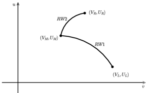
Figure 5: Admissible connection between rarefaction wave curves of the first and second families

• Region $I$: The states $(U_{L},q_{L})$ and $(U_{R},q_{R})$ are connected by a combination of RW1 and RW2 via the state $(U_{M},q_{M})$. In this situation, we do not have any Rankine-Hugoniot deficit since the solution $(u,q)$ to (16) is continuous. Thus, we simply write $(u,v)=(u,\sqrt{2q-u^{2}})$ and this is the solution to (1), (2). The solution is plotted in Figure 5.

  As for the uniqueness, we know that the function $u$ is unique since it is the Lax admissible solution to (16) with the initial data (34). The function $v$ is determined by the unique functions $u$ and $q$ via

  $$v=\pm\sqrt{2q-u^{2}}.$$

  Thus, $v$ could change sign so that we connect $V_{L}$ by $V_{M1}$ and then skip to $-V_{M1}$ on $v=-\sqrt{2q-u^{2}}$ and then connect it by $-V_{M2}$. From here we connect to $V_{M2}$ located on the original curve $v=\sqrt{2q-u^{2}}$ and then connect $V_{M2}$ to $V_{M}$. Finally, we connect $V_{M}$ with $V_{R}$. The procedure is illustrated in Figure 6. However, since we imposed the requirement that the solutions have a minimal number of $\delta$-distributions and we cannot connect the states $(U_{M1},V_{M1})$ and $(U_{M1},-V_{M1})$ using the $\delta$-shock since such a choice would yield a solutions with a higher number of singular parts than the previously described solution.

  Thus the shock connecting the states $(U_{M1},V_{M1})$ and $(U_{M1},-V_{M1})$ cannot be singular, (i.e. there can be no Rankine-Hugoniot deficit), and therefore the speed $s$ of the shock must satisfy the Rankine-Hugoniot condition

  $$s=U_{M1}.$$

  On the other hand, the characteristic speeds of $(U_{M1},V_{M1})$ and $(U_{M1},-V_{M1})$ are $\lambda_{1}(U_{M1},V_{M1})=\lambda_{1}(U_{M1},-V_{M1})\neq s$, and since these are equal, the shock connection between $(U_{M1},V_{M1})$ and $(U_{M1},-V_{M1})$ is impossible with Rankine-Hugoniot condition satisfied.

  Similarly, the same requirement makes it impossible to connect $(U_{M2},V_{M2})$ and $(U_{M2},-V_{M2})$ by a $\delta$-shock. In this case, the shock speed satisfies the Rankine-Hugoniot condition

  $$s=U_{M2}.$$

  Furthermore, we have equality of speeds $\lambda_{2}(U_{M2},V_{M2})=\lambda_{2}(U_{M2},-V_{M2})$, but we have the contrasting inequality $\lambda_{2}(U_{M2},V_{M2})=\lambda_{2}(U_{M2},-V_{M2})\neq s$ implying that a shock connection between $(U_{M2},V_{M2})$ and $(U_{M2},-V_{M2})$ is not possible if the Rankine-Hugoniot condition is satisfied. The same procedure leads to the conclusion that a $\delta$-shock connection between $(U_{M},V_{M})$ and $(U_{M},-V_{M})$ is impossible with Rankine-Hugoniot condition satisfied.

  Hence, the only possible connection of $(U_{L},V_{L})$ and $(U_{R},V_{R})$ is by the combination RW1 and RW2 via the state $(U_{M},V_{M})$. Consequently, we remark that RW1 and RW2 corresponding to (16) are transformed via $(u,q)\mapsto(u,\sqrt{2q-u^{2}})$ into RW1 and RW2 corresponding to (1) (since $q$ is the entropy function for (1), and RW1 and RW2 are smooth solutions to (16)).

  

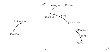
  Figure 6: Nonadmissible connection between rarefaction wave curves of the first and the second families

• Region $II$: The states $(U_{L},q_{L})$ and $(U_{R},q_{R})$ are connected by the combination SW1 and RW2 via the state $(U_{M},q_{M})$.

  Unlike the previous case, we have a shock wave in (16), and we will necessarily have a Rankine-Hugoniot deficit in the original system (1). We thus define

  $$(u,v)=(u,\sqrt{2q-u^{2}})+(0,\beta(t)\delta(x-ct)),$$ (35)

  where $c$ is the speed of the SW1 connecting the states $(U_{L},q_{L})$ and $(U_{M},q_{M})$ in (16). The speed $c$ is given by (11) as well as the corresponding Rankine-Hugoniot deficit $\beta(t)$:

  $$c=\frac{\frac{U_{L}^{2}+V_{L}^{2}}{2}-\frac{U_{R}^{2}+V_{R}^{2}}{2}}{U_{L}-U_{R}},\ \ \beta(t)=(c(V_{L}-V_{R})-(V_{L}(U_{L}-1)-V_{R}(U_{R}-1))t.$$ (36)

  Concerning the other possible solutions, as in the previous item, we can only split the curve connecting $(U_{L},V_{L})$ and $(U_{M},V_{M})$ into several new curves e.g. by connecting the states $(U_{L},V_{L})$ and $(U_{M1},V_{M1})$, then the (opposite with respect to $v$) states $(U_{M1},V_{M1})$ and $(U_{M1},-V_{M1})$, then $(U_{M1},-V_{M1})$ and $(U_{M2},-V_{M2})$, then $(U_{M2},-V_{M2})$ and $(U_{M2},V_{M2})$ etc. until we reach $(U_{M},V_{M})$. The states $(U_{M1},V_{M1})$ and $(U_{M1},-V_{M1})$ can be connected only by the shock satisfying the Rankine-Hugoniot conditions (due to the minimality condition on $\delta$-shocks, we cannot have a Rankine-Hugoniot deficit).

  Since we cannot have the Rankine-Hugoniot deficit, as in the previous item, we must connect the various states with shock waves satisfying the Rankine-Hugoniot conditions, and at the same time being equal to the speed $c$ (the speed of the SW1 connecting the states $(U_{L},q_{L})$ and $(U_{M},q_{M})$ in (16)). This is obviously never fulfilled i.e. the only solution in this case is (35).

• Region $III$:

  The states $(U_{L},q_{L})$ and $(U_{R},q_{R})$ are connected by the combination RW1 and SW2 via the state $(U_{M},q_{M})$.

  The analysis for the existence and uniqueness proceeds along the same lines as the first two cases. The admissible (and thus unique) $\delta$-type solution in this case has the form:

  $$(u,v)=\big{(}u,\sqrt{2q-u^{2}}\big{)}+\big{(}0,\beta(t)\delta(x-ct)\big{)},$$ (37)

  where $c$ in this case represents the speed of the SW2 connecting the states $(U_{R},q_{R})$ and $(U_{M},q_{M})$ in (16). The speed $c$ and the corresponding Rankine-Hugoniot deficit $\beta(t)$ are given in (11) and explicitly expressed as in (36). The solution structure is represented by

  $$(U_{L},V_{L})\xrightarrow{RW1}(U_{M},V_{M})\xrightarrow{SW2}(U_{R},V_{R}),$$

  where the $\delta$-shock propagates at the speed $c=\lambda_{1}(U_{M},V_{M})=\lambda_{1}(U_{M},-V_{M})$. Notice that it is possible to generate infinitely many non-admissible (in the sense of Definition 3.1) solutions (in the sense of Definition 1.1) by partitioning the rarefaction wave of the first family that connects the states $(U_{L},V_{L})$ and $(U_{M},V_{M})$. The solution is constructed by connecting $(U_{L},V_{L})$ and $(U_{M1},V_{M1})$ by RW1 and then passing over to $(U_{M1},-V_{M1})$ by a shock which satisfies the Rankine-Hugoniot conditions $s=U_{M1}$. The procedure is advanced to connect all the finite possible states $(U_{Mk},V_{Mk})$ and $(U_{Mk},-V_{Mk})$ by a shock satisfying both the Rankine-Hugoniot conditions $s=U_{Mk}$, where $k\in\mathbb{Z}_{+}$ and the speed of the shock of the second family connecting the states $(U_{M},-V_{M})$ and $(U_{R},V_{R})$. This process is carried out prior to the state $(U_{M},V_{M})$ and the shocks connecting pairs of states cannot be admissible in the sense of Definition 3.1 due to the minimality condition. Consequently, the only solution admissible in this sense is (37).

• Region $IV$: The states $(U_{L},q_{L})$ and $(U_{R},q_{R})$ are connected by the combination SW1 and SW2 via the state $(U_{M},q_{M})$.

  The presence of shocks in this case will necessarily introduce Rankine-Hugoniot deficit in (1). The solution is constructed by solving (16) for the solution $(u,q)$ and then go back to (1) to obtain the admissible $\delta$-type solution

  $$(u,v)=\big{(}u,\sqrt{2q-u^{2}}\big{)}+\big{(}0,\beta_{1}(t)\delta(x-c_{1}t)\big{)}+\big{(}0,\beta_{2}(t)\delta(x-c_{2}t)\big{)},$$ (38)

  where $c_{1}$ and $c_{2}$ given by the expressions

  $$c_{1}=\frac{\frac{U_{L}^{2}+V_{L}^{2}}{2}-\frac{U_{M}^{2}+V_{M}^{2}}{2}}{U_{L}-U_{M}}\ \ \ \ \text{and}\ \ \ \ \ c_{2}=\frac{\frac{U_{M}^{2}+V_{M}^{2}}{2}-\frac{U_{R}^{2}+V_{R}^{2}}{2}}{-U_{M}-U_{R}},$$ (39)

  are the speeds of the shocks SW1 and SW2 respectively. The Rankine-Hugoniot deficits $\beta_{1}(t)$ and $\beta_{2}(t)$ are expressed as in (36) for the appropriate states. The analysis for uniqueness of (38) is similar to the above cases except that all the elementary waves involved in this case are shocks.

Now, assume that $V_{L}>0$ and $V_{R}<0$. It was shown in [8] that in this case, the Riemann problem (1), (2) does not admit a Lax admissible solution, even for initial data with small variation.

In order to get an admissible $\delta$-type solution, as before, we solve (16) with $(U_{0},q_{0})$ as the initial data. The obtained solution connects $(U_{L},q_{L})$ with $(U_{R},q_{R})$ by Lax admissible waves through a middle state $(U_{M},q_{M})$. Next, we go back to the original system (1) by connecting $(U_{L},V_{L})$ with $(U_{M},\sqrt{2q_{M}-U_{M}^{2}})$ by an elementary wave containing the corresponding Rankine-Hugoniot deficit corrected by the $\delta$-shock wave. Then, we connect $(U_{M},\sqrt{2q_{M}-U_{M}^{2}})$ with $(U_{M},-\sqrt{2q_{M}-U_{M}^{2}})$ by the shock wave whose speed will obviously be $U_{M}$. Finally, we connect $(U_{M},-\sqrt{2q_{M}-U_{M}^{2}})$ with $(U_{R},V_{R})$ by an elementary wave containing corresponding Rankine-Hugoniot deficit corrected by the $\delta$-shock wave.

Let us first show it is possible to apply the described procedure. We again need to split considerations into four possibilities depending on how the states $(U_{L},q_{L})$ and $(U_{R},q_{R})$ are connected.

Figure 7: Admissible connection between rarefaction wave curves of the first and second families in the case when the left state has $V_{L}<0$ and the right state has $V_{R}>0$. In this case, a shock connecting the states $(-V_{M},U_{M})$ and $(V_{M},U_{M})$ has to be fitted between the rarefaction curves. It is shown in the part of the proof pertaining to region I that this shock has the required speed.

• Region $I$: The states $(U_{L},q_{L})$ and $(U_{R},q_{R})$ are connected by RW1 and RW2 via the middle state $(U_{M},q_{M})$.

  It is clear that we can connect $(U_{L},V_{L})$ with $(U_{M},\sqrt{2q_{M}-U_{M}^{2}})$ using RW1 (it is the same for both equations since RW1 and RW2 are smooth solutions to (16)). Also, we can connect $(U_{M},-\sqrt{2q_{M}-U_{M}^{2}})$ with $(U_{R},V_{R})$ using RW2. We need to prove that the shock wave connecting $(U_{M},\sqrt{2q_{M}-U_{M}^{2}})$ and $(U_{M},-\sqrt{2q_{M}-U_{M}^{2}})$ has a speed which is between $\lambda_{1}(U_{M},\sqrt{2q_{M}-U_{M}^{2}})$ and $\lambda_{2}(U_{M},-\sqrt{2q_{M}-U_{M}^{2}})$.

  In other words, we need to check

  $$U_{M}-\frac{1}{2}-\sqrt{V_{M}^{2}+{\textstyle\frac{1}{4}}}\leq U_{M}\leq U_{M}-\frac{1}{2}+\sqrt{V_{M}^{2}+{\textstyle\frac{1}{4}}}$$

  which is obviously correct. This configuration is depicted in Figure 7.

• Region $II$:

  The states $(U_{L},q_{L})$ and $(U_{R},q_{R})$ are connected by SW1 and SW2 via the middle state $(U_{M},q_{M})$.

  As in the previous item, we connect $(U_{L},V_{L})$ with $(U_{M},\sqrt{2q_{M}-U_{M}^{2}})$ this time using the SW1 from (16) which will induce the Rankine-Hugoniot deficit in (1). Then, we skip from $(U_{M},\sqrt{2q_{M}-U_{M}^{2}})$ to $(U_{M},-\sqrt{2q_{M}-U_{M}^{2}})$ using the standard shock wave (the one satisfying the Rankine-Hugoniot conditions), and finally we go from $(U_{M},-\sqrt{2q_{M}-U_{M}^{2}})$ to $(U_{R},V_{R})$ using the SW2 from (16) and corrected with an appropriate $\delta$-shock. More precisely, the admissible $\delta$-type solution will have the form:

  $$\begin{split}u(t,x)&=U_{L}+(U_{M}-U_{L})(H(x-c_{1}t)-H(x-ct))\\ &+(-U_{M}-U_{L})(H(x-ct)-H(x-c_{2}t))+(U_{R}-U_{L})H(x-c_{2}t)\\ v(t,x)&=V_{L}+(V_{M}-V_{L})(H(x-c_{1}t)-H(x-ct))\\ &+(V_{M}-V_{L})(H(x-ct)-H(x-c_{2}t))+(V_{R}-V_{L})H(x-c_{2}t)\\ &+\beta_{1}(t)\delta(x-c_{1}t)+\beta_{2}(t)\delta(x-c_{2}t),\end{split}$$ (40)

  where $c_{1}$ is the speed of the SW1 connecting $(U_{L},q_{L})$ with $(U_{M},q_{M})$ in (16), $c_{2}$ is the speed of the SW2 connecting $(U_{M},q_{M})$ with $(U_{R},q_{R})$ in (16), while $c$ is the speed of the shock connecting $(U_{M},-\sqrt{2q_{M}-U_{M}^{2}})$ with $(U_{M},\sqrt{2q_{M}-U_{M}^{2}})$ and it is given by the Rankine-Hugoniot conditions from (1). The deficits $\beta_{1}$ and $\beta_{2}$ are given by Theorem 1.2 (see (36) for the analogical situation).

  However, we still need to prove that (40) is well defined, i.e. that

  $$c_{1}\leq c\leq c_{2}\ \ \implies$$

  $$\frac{2U_{M}-1-\sqrt{8q_{L}+1+\frac{4U_{M}^{2}}{3}-\frac{8U_{L}U_{M}}{3}-\frac{8U_{L}^{2}}{3}-2U_{M}+2U_{L}}}{2}\leq U_{M}$$

  $$\leq\frac{2U_{M}-1+\sqrt{8q_{R}+1+\frac{4U_{M}^{2}}{3}-\frac{8U_{M}U_{R}}{3}-\frac{8U_{R}^{2}}{3}-2U_{M}+2U_{R}}}{2}$$

  which is also clearly true.

• Region $III$: The states $(U_{L},q_{L})$ and $(U_{R},q_{R})$ are connected by RW1 and SW2 via the middle state $(U_{M},q_{M})$.

  This case, as well as the following one, is handled by combining the previous two cases.

• Region $IV$:

  The states $(U_{L},q_{L})$ and $(U_{R},q_{R})$ are connected by SW1 and RW2 via the middle state $(U_{M},q_{M})$.

Uniqueness is obtained by arguing as in the first part of the proof.

∎

References

- [1] M. Brio, Admissibility conditions for weak solutions to non-strictly hyperbolic systems, J.Ballmann et al. (eds.), Nonlinear Hyperbolic Equations – Theory, Computation methods and Applications, 1989. Friedr. Vieweg and Sohn Verlagsgesellschaft mbH, Braunschweig.
- [2] S. Bianchini, A. Bressan, Vanishing viscosity solutions of nonlinear hyperbolic systems, Ann. of Math. 161 (2005), 223–352.
- [3] C. Dafermos, Hyperbolic Conservation Laws in Continuum Physics, Springer,Grundlehren der mathematischen Wissenschaften, Vol. 325.
- [4] G. Dal Maso, P. LeFloch and F. Murat, Definition and weak stability of non-conservative products, J. Math. Pures Appl. 74 (1995), 483–548.
- [5] V.G. Danilov, G.A. Omel’yanov, V.M. Shelkovich, Weak asymptotic methods and interaction of nonlinear waves, Asymptotic methods for wave and quantum problems (ed. M. V. Karasev), American Mathematical Translations Series 2, Vol. 208, RI: American Mathematical Society, Providence,2003), 33–165.
- [6] V. G. Danilov and V. M. Shelkovich, Dynamics of propagation and interaction of -shock waves in conservation law system, J. Differential Equations 211 (2005), 333–381.
- [7] S. Gavrilyuk, H. Kalisch and Z. Khorsand. A kinematic conservation law in free surface flow, Nonlinearity 28 (2015), 1805–1821.
- [8] B. Hayes and P. G. LeFloch, Measure-solutions to a strictly hyperbolic system of conservation laws, Nonlinearity 9 (1996), 1547–1563.
- [9] F. Huang, Existence and uniqueness of discontinuous solutions for a hyperbolic system, Proc. Roy. Soc. Edinburgh 127 (1997), 1193–1205.
- [10] F. Huang, Z. Wang, Well posedeness for pressureless flow, Comm. Math. Phys. 222 (2001), 117–146.
- [11] H. Kalisch and D. Mitrović, Singular solutions of a fully nonlinear system of conservation laws, Proc. Edinb. Math. Soc. 55 (2012), 711–729.
- [12] H. Kalisch, D. Mitrovic and V. Teyekpiti, Delta shock waves in shallow water flow, Phys. Lett. A 381 (2017), 1138–1144.
- [13] H. Kalisch and V. Teyekpiti, A shallow-water system with vanishing buoyancy, submitted.
- [14] B. Keyfitz, C. Tsikkou, Conserving the wrong variables in gas dynamics: a Riemann solution with singular shocks, Quart. Appl. Math. 70 (2012), no. 3, 407–436.
- [15] B. Keyfitz, H. Kranzer, Spaces of weighted measures for conservation laws with singular shock solutions, J. Differential Equations 118 (1995), 420–451.
- [16] C. Korchinski, Solution of a Riemann problem for a system of conservation laws possessing no classical weak solution, PhD Thesis, Adelphi University, 1977.
- [17] P.D. Lax, Hyperbolic systems of conservation laws II, Comm. Pure Appl. Math. 10 (1957), 537–566.
- [18] T.P. Liu, The entropy condition and the admissibility of shocks, J. Math. Anal. Appl. 53 (1976), 78–88.
- [19] M. Mazzotti, A. Tarafder, J. Cornel, F. Gritti and G. Guiochon, Experimental evidence of a -shock in nonlinear chromatography, J. Chromatography. A, 1217 (2010), 2002–2012.
- [20] M. Nedeljkov, Higher order shadow waves and delta shock blow up in the Chaplygin gas, J. Differential Equations 256 (2014), 3859–3887.
- [21] M. Nedeljkov, Shadow Waves: Entropies and Interactions for Delta and Singular Shocks, Arch. Ration. Mech. Anal. 197 (2010), 489–537.
- [22] G.A. Omelyanov About the stability problem for strictly hyperbolic systems of conservation laws, Rend. Sem. Mat. Univ. Politec. Torino 69 (2011), 377–392.
- [23] C.O.R. Sarrico, The Riemann problem for the Brio system: a solution containing a Dirac mass obtained via a distributional product, Russ. J. Math. Phys. 22 (2015), 518–527.
- [24] M. Sun, Delta shock waves for the chromatography equations as self-similar viscosity limits, Quarterly of Applied Mathematics 69 (2011), 425-443.
- [25] C. Tsikkou, Hyperbolic conservation laws with large initial data. Is the Cauchy problem well-posed?, Quart. Appl. Math. 68 (2010), 765–781.
- [26] G. Wang, One-dimensional nonlinear chromatography system and delta-shock waves, Z. Angew. Math. Phys. 64 (2013), 1451–1469.