A new approach to Lickorish-Millett type formulae

Abstract.

In this paper, we introduce a new method to prove the Lickorish-Millett type formulae for colored HOMFLY-PT polynomials of links.

1. Introduction

The HOMFLY-PT polynomial is a two variables link invariant that was first discovered by Freyd-Yetter, Lickorish-Millett, Ocneanu, Hoste and Przytycki-Traczyk. Given an oriented link $\mathcal{L}$ in $S^{3}$, its HOMFLY-PT polynomial $P(\mathcal{L},q,t)$ satisfies the following skein relation,

(1.1) $$tP(\mathcal{L}_{+};q,t)-t^{-1}P(\mathcal{L}_{-};q,t)=(q-q^{-1})P(\mathcal{L}_{0};q,t)$$

where we will use the notation $(\mathcal{L}_{+},\mathcal{L}_{-},\mathcal{L}_{0})$ to denote the Conway triple throughout this paper. Given an initial value $P(U;q,t)=1$ for an unknot $U$, one can compute the HOMFLY-PT polynomial for a given oriented link recursively through the above formula (1.1). We can give the definition of the HOMFLY-PT polynomial through the HOMFLY-PT skein of the plane $\mathcal{S}(\mathbb{R}^{2})$. Any link diagram of a link $\mathcal{L}$ in $\mathcal{S}(\mathbb{R}^{2})$ will be equal to a scalar denoted by $\mathcal{H}(\mathcal{L};q,t)$. In particular, for an unknot $U$, $\mathcal{H}(U;q,t)=\frac{t-t^{-1}}{q-q^{-1}}$. Then the HOMFLY-PT polynomial of $\mathcal{L}$ is defined by

(1.2) $$P(\mathcal{L};q,t)=\frac{t^{-w(\mathcal{L})}\mathcal{H}(\mathcal{L};q,t)}{\mathcal{H}(U;q,t)},$$

where $w(\mathcal{L})$ is the writhe number of $\mathcal{L}$. In Section 2, by a simple observation, we obtain the following structural theorem for HOMFLY-PT polynomials first showed by Lickorish-Millett in [4].

Proposition 1.1.

For a link $\mathcal{L}$ with $L$ components, we have the following expansions:

(1.3) $$\mathcal{H}(\mathcal{L};q,t)=\sum_{g\geq 0}h_{2g-L}^{\mathcal{L}}(t)z^{2g-L},$$

(1.4) $$P(\mathcal{L};q,t)=\sum_{g\geq 0}p_{2g+1-L}^{\mathcal{L}}(t)z^{2g+1-L},$$

where $z=q-q^{-1}$. The polynomials $h_{2g-L}^{\mathcal{L}}(t)$ and $p_{2g+1-L}^{\mathcal{L}}(t)$ will be called coefficient polynomials. According to the formula (1.2), it clear that we have the relations

(1.5) $$h_{2g-L}^{\mathcal{L}}(t)=p_{2g+1-L}^{\mathcal{L}}(t)t^{w(\mathcal{L})}(t-t^{-1}),$$

for $g\geq 0$.

Furthermore, Lickorish-Millett [4] first studied the explicit expressions of the coefficient polynomials $p_{2g+1-L}^{\mathcal{L}}(t)$ appearing in the above expansions (1.4). They studied the first coefficient $p_{1-L}^{\mathcal{L}}(t)$ for a link $\mathcal{L}$ with $L$ components and obtained the following Theorem 1.4. Then in [3], Kanenobu-Miyazawa carefully computed the second and third coefficients $p_{3-L}^{\mathcal{L}}(t)$, $p_{5-L}^{\mathcal{L}}(t)$ by using the similar method as in [4]. All these formulas about the coefficient polynomials $p_{2g+1-L}^{\mathcal{L}}(t)$ will be called the ”Lickorish-Millett” type formulas. In this paper, we introduce a completely new method to study these coefficient polynomials $p_{2g+1-L}^{\mathcal{L}}(t)$. This method is motivated by the work of [6] in the proof of Labastida-Mariño-Ooguri-Vafa (LMOV) conjecture.

Let us fix some notation. For a link $\mathcal{L}$ with $L$ components, let $\mathbf{I}$ be a subset of $\mathbf{L}=\{1,2,...,L\}$. Denote by $\mathcal{L}_{\mathbf{I}}$ the sub-link obtained by removing the components whose sub-indices are not contained in $\mathbf{I}$. For example, if $\mathcal{L}$ is a link of two components $\mathcal{K}_{1}$ and $\mathcal{K}_{2}$, then $\mathcal{L}_{\{2\}}=\mathcal{K}_{2}$. For $L\geq 1$ and $l\leq L$, we will use the notation $\cup_{s=1}^{l}\mathbf{I}_{s}=\mathbf{L}$ to denote a nonempty disjoint ordered decomposition of the set $\mathbf{L}=\{1,..,L\}$, i.e. every $\mathbf{I}_{s}\subset\mathbf{L}$, $\mathbf{I}_{s}\neq\emptyset$ and $\mathbf{I}_{s}\cap\mathbf{I}_{t}=\emptyset$ for $s\neq t$ such that $\mathbf{I}_{1}\cup\mathbf{I}_{2}\cup\cdots\cup\mathbf{I}_{l}=\mathbf{L}$, and different orders of $\mathbf{I}_{1},\mathbf{I}_{2},\cdots,\mathbf{I}_{l}$ give different decompositions.

We introduce the intermediate invariant $\mathcal{F}(\mathcal{L};q,t)$ as follow:

(1.6) $$\mathcal{F}(\mathcal{L};q,t)=\sum_{l=1}^{L}\frac{(-1)^{l-1}}{l}\sum_{\cup_{s=1}^{l}\mathbf{I}_{s}=\mathbf{L}}\prod_{s=1}^{l}\mathcal{H}(\mathcal{L}_{\mathbf{I}_{s}};q,t),$$

where the summation $\sum_{\cup_{s=1}^{l}\mathbf{I}_{s}=\mathbf{L}}$ denotes the sum over all nonempty disjoint ordered decompositions $\cup_{s=1}^{l}\mathbf{I}_{s}=\mathbf{L}$ throughout this paper.

In Section 3, we will prove that

Proposition 1.2.

(1.7) $$\deg_{z}\mathcal{F}(\mathcal{L};q,t)\geq L-2.$$

where we use the notation $\deg_{z}f$ to denote the lowest degree of $z$ in a polynomial $f\in z^{-L}\mathbb{Q}[z^{2},t^{\pm 1}]$.

Combining the expansion formula (1.3) for $\mathcal{H}(\mathcal{L};q,t)$ and Proposition 1.2, we immediately have

Theorem 1.3.

For a link $\mathcal{L}$ with $L$ components, the coefficient polynomials $h_{2g-L}^{\mathcal{L}}(t)$ for $g=0,..,L-2$ can be expressed as follow:

(1.8) $$h_{2g-L}^{\mathcal{L}}(t)=\sum_{l=2}^{L}\frac{(-1)^{l}}{l}\sum_{\sum_{s=1}^{l}g_{s}=g}\sum_{\cup_{s=1}^{l}\mathbf{I}_{s}=\mathbf{L}}\prod_{s=1}^{l}h_{2g_{s}-I_{s}}^{\mathcal{L}_{\mathbf{I}_{s}}}(t).$$

where the second summation $\sum_{\sum_{s=1}^{l}g_{s}=g}$ denotes the sum over all nonnegative integers $g_{1},g_{2}...,g_{l}$ such that $\sum_{s=1}^{l}g_{s}=g$.

In fact, by using the relation (1.5), Theorem 1.3 directly gives us $L-1$ Lickorish-Millett type formulas for the coefficient polynomials $p_{2g+1-L}^{\mathcal{L}}(t)$, $g=0,1,...,L-2$.

For examples, when $g=0$, we reprove the following result due to Lickorish-Millett ( See Proposition 22 in [4]).

Theorem 1.4.

The first coefficient $p_{1-L}^{{\mathcal{L}}}(t)$ in the expansion

(1.9) $$P(\mathcal{L};q,t)=\sum_{g\geq 0}p_{2g+1-L}^{{\mathcal{L}}}(t)z^{2g+1-L}$$

is given by

(1.10) $$p_{1-L}^{{\mathcal{L}}}(t)=t^{-2lk({\mathcal{L}})}(t-t^{-1})^{L-1}\prod_{\alpha=1}^{L}p_{0}^{{\mathcal{K}}_{\alpha}}(t),$$

where $lk({\mathcal{L}})$ is the linking number of $\mathcal{L}$.

When $g=1$, we recover the following theorem of Kanenobu-Miyazawa (See Theorem 1.1 in [3]).

Theorem 1.5.

The second coefficient $p_{3-L}^{{\mathcal{L}}}(t)$ in the HOMFLY-PT polynomial

(1.11) $$P(\mathcal{L};q,t)=\sum_{g\geq 0}p_{2g+1-L}^{{\mathcal{L}}}(t)z^{2g+1-L}$$

is given by

(1.12) $$p_{3-L}^{{\mathcal{L}}}(t)= t^{-2lk({\mathcal{L}})}\left((t-t^{-1})^{L-2}\sum_{1\leq\beta<\gamma\leq L}t^{2lk({\mathcal{L}}_{(\alpha\beta)})}p_{1}^{{\mathcal{L}}_{(\alpha\beta)}}(t)\prod_{\alpha\neq\beta,\gamma}p_{0}^{{\mathcal{K}}_{\alpha}}(t)\right.$$

$$\left.-(L-2)(t-t^{-1})^{L-1}\sum_{\beta=1}^{L}p_{2}^{{\mathcal{K}}_{\alpha}}(t)\prod_{\alpha\neq\beta}p_{0}^{{\mathcal{K}}_{\alpha}}(t)\right).$$

By using Theorem 1.3, we reduce the proofs of Theorem 1.4 and Theorem 1.5 to some combinatorial identities which will be shown in Section 5.

Finally, in the appendix, for the reader’s convenience, we describe the classical approach to Theorem 1.4 and Theorem 1.5 as shown in [4] and [3] with a slightly different method.

Acknowledgements. This paper grows out of an old note by the second author when he learned of the Labastida-Mariño-Ooguri-Vafa question from Prof. Kefeng Liu. He would like to thank Prof. Kefeng Liu for sharing with him many new ideas. He also appreciates the collaboration with Qingtao Chen, Kefeng Liu and Pan Peng in this area and many valuable discussions with them within the past years. The authors are grateful to the referees for their valuable comments and suggestions which greatly improved the presentation of the content.

The research of S. Zhu is supported by the National Science Foundation of China grant No. 11201417 and the China Postdoctoral Science special Foundation No. 2013T60583.

2. HOMFLY-PT polynomials

The HOMFLY-PT polynomial of an oriented link $\mathcal{L}$ can be defined by using the framed HOMFLY-PT skein of the plane $\mathcal{S}(\mathbb{R}^{2})$ which is the set of linear combinations of oriented link diagrams, modulo two relations given in Figure 1, where $z=q-q^{-1}$.

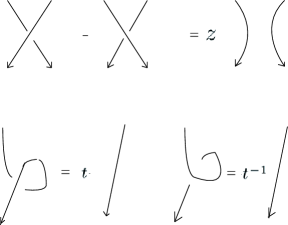
Figure 1.

It is easy to follow that the removal an unknot requires a multiplication by the scalar $s=\frac{t-t^{-1}}{q-q^{-1}}$, i.e we have the relation showed in Figure 2.

Figure 2.

The planar projection of an oriented link, $\mathcal{L}$, gives an oriented diagram that is denoted by $D_{\mathcal{L}}$. By using the above two relations, any diagram $D_{\mathcal{L}}$ is equal to a scalar. We denote the resulting scalar by $\langle D_{\mathcal{L}}\rangle\in\Lambda$. Then the (framed unreduced) HOMFLY-PT polynomial $\mathcal{H}(\mathcal{L};q,t)$ of the link $\mathcal{L}$ is defined by $\mathcal{H}(\mathcal{L};q,t)=\langle D_{\mathcal{L}}\rangle$. We use the convention $\langle\ \rangle=1$ for the empty diagram, for the unknot $U$, $\mathcal{H}(U;q,t)=\frac{t-t^{-1}}{q-q^{-1}}$. The two relations shown in Figure 1 lead to

(2.1) $$\mathcal{H}(\mathcal{L}_{+};q,t)-\mathcal{H}(\mathcal{L}_{-};q,t)=z\mathcal{H}(\mathcal{L}_{0};q,t),$$

(2.2) $$\mathcal{H}(\mathcal{L}^{+1};q,t)=t\mathcal{H}(\mathcal{L};q,t),\ \mathcal{H}(\mathcal{L}^{-1};q,t)=t^{-1}\mathcal{H}(\mathcal{L};q,t).$$

The classical HOMFLY-PT polynomial of a link $\mathcal{L}$ is given by

(2.3) $$P(\mathcal{L};q,t)=\frac{t^{-w(\mathcal{L})}\mathcal{H}(\mathcal{L};q,t)}{\mathcal{H}(U;q,t)}.$$

By the observation used in [2], for a link $\mathcal{L}$ with $L$ components, we introduce the link polynomial $\check{\mathcal{H}}(\mathcal{L};q,t)$ defined as

(2.4) $$\check{\mathcal{H}}(\mathcal{L};q,t)=z^{L}\mathcal{H}(\mathcal{L};q,t).$$

By comparing the numbers of components of links $\mathcal{L}_{+},\mathcal{L}_{-},\mathcal{L}_{0}$ in Conway triple, the relations (2.1) and (2.2) of $\mathcal{H}(\mathcal{L};q,t)$ give us

(2.5) $$\check{\mathcal{H}}(\mathcal{L}_{+};q,t)-\check{\mathcal{H}}(\mathcal{L}_{-};q,t)=z^{2\epsilon}\check{\mathcal{H}}(\mathcal{L}_{0};q,t)$$

(2.6) $$\check{\mathcal{H}}(\mathcal{L}^{+1};q,t)=t\check{\mathcal{H}}(\mathcal{L};q,t),\ \check{\mathcal{H}}(\mathcal{L}^{-1};q,t)=t^{-1}\check{\mathcal{H}}(\mathcal{L};q,t)$$

where $\epsilon=0$ if the crossing is a self-crossing of a knot, $\epsilon=1$ if this crossing is a crossing between two components of a link. Let $U$ be the unknot, we have $\check{\mathcal{H}}(U;q,t)=t-t^{-1}$. By using the relations (2.5) and (2.6) recursively, we have

Lemma 2.1.

For any link $\mathcal{L}$, $\check{\mathcal{H}}(\mathcal{L};q,t)\in\mathbb{Z}[z^{2},t^{\pm 1}]$.

In other words, for a link $\mathcal{L}$, there are polynomials of $t$ denoted by $\check{h}_{g}^{\mathcal{L}}(t)\in\mathbb{Z}[t^{\pm 1}]$, such that $\check{\mathcal{H}}(\mathcal{L};q,t)$ has the following expansion:

(2.7) $$\check{\mathcal{H}}(\mathcal{L};q,t)=\sum_{g\geq 0}\check{h}_{g}^{\mathcal{L}}(t)z^{2g}.$$

It immediately implies the following structural formulae for $\mathcal{H}(\mathcal{L};q,t)$ and $P(\mathcal{L};q,t)$.

Proposition 2.2.

For a link $\mathcal{L}$ with $L$ components

(2.8) $$\mathcal{H}(\mathcal{L};q,t)=\sum_{g\geq 0}h_{2g-L}^{\mathcal{L}}(t)z^{2g-L},$$

(2.9) $$P(\mathcal{L};q,t)=\sum_{g\geq 0}p_{2g+1-L}^{\mathcal{L}}(t)z^{2g+1-L},$$

where $h_{2g-L}^{\mathcal{L}}(t)=\check{h}_{g}^{\mathcal{L}}(t)$, and $p_{2g+1-L}^{\mathcal{L}}(t)=\frac{t^{-w(\mathcal{L})}h_{2g-L}^{\mathcal{L}}(t)}{t-t^{-1}}$

We remark that the formula (2.9) was first showed in the paper [4].

3. An intermediate invariant

In this section, we introduce an intermediate invariant whose properties imply the Lickorish-Millett type formulae. With the same notations shown in Section 1, the intermediate invariant $\mathcal{F}(\mathcal{L};q,t)$ is given by the formula (1.6)

(3.1) $$\mathcal{F}(\mathcal{L};q,t)=\sum_{l=1}^{L}\frac{(-1)^{l-1}}{l}\sum_{\cup_{s=1}^{l}\mathbf{I}_{s}=\mathbf{L}}\prod_{s=1}^{l}\mathcal{H}(\mathcal{L}_{\mathbf{I}_{s}};q,t).$$

By formula (2.8) in Proposition 2.2, it is obvious that

(3.2) $$\mathcal{F}(\mathcal{L};q,t)\in z^{-L}\mathbb{Q}[z^{2},t^{\pm 1}].$$

In fact, we have a more precise structure for $\mathcal{F}(\mathcal{L};q,t)$.

Proposition 3.1.

If we use the notation $\deg_{z}f$ to denote the lowest degree of $z$ in a polynomial $f\in z^{-L}\mathbb{Q}[z^{2},t^{\pm 1}]$.

(3.3) $$\deg_{z}\mathcal{F}(\mathcal{L};q,t)\geq L-2.$$

Proof.

For a link $\mathcal{L}$ with $L$ components, $\mathcal{K}_{\alpha},\alpha=1,..,L$. Let us consider a crossing which is a crossing between two different components $\mathcal{K}_{\alpha}$ and $\mathcal{K}_{\beta}$ of $\mathcal{L}$, we have

(3.4) $$\mathcal{F}(\mathcal{L}_{+};q,t)-\mathcal{F}(\mathcal{L}_{-};q,t)$$

$$=\sum_{l=1}^{L}\frac{(-1)^{l-1}}{l}\sum_{\cup_{s=1}^{l}\mathbf{I}_{s}=\mathbf{L}}\left(\prod_{s=1}^{l}\mathcal{H}((\mathcal{L}_{+})_{\mathbf{I}_{s}};q,t)-\prod_{s=1}^{l}\mathcal{H}((\mathcal{L}_{-})_{\mathbf{I}_{s}};q,t)\right)$$

Note that on the right hand side of the above formula, only the terms that contain the crossings in the same sub-link $\mathcal{L}_{\mathbf{I}_{s}}$ survive. By skein relation (2.1), one has

(3.5) $$\mathcal{F}(\mathcal{L}_{+};q,t)-\mathcal{F}(\mathcal{L}_{-};q,t)=z\mathcal{F}(\mathcal{L}_{0};q,t).$$

For brevity, we introduce the following notation for a link $\mathcal{L}$ with $L$ components

(3.6) $$\hat{\mathcal{F}}(\mathcal{L};q,t)=\frac{\mathcal{F}(\mathcal{L};q,t)}{z^{L}}.$$

So we only need to prove

(3.7) $$\deg_{z}\hat{\mathcal{F}}(\mathcal{L};q,t)\geq-2.$$

We see that the formula (3.5) becomes

(3.8) $$\hat{\mathcal{F}}(\mathcal{L}_{+};q,t)-\hat{\mathcal{F}}(\mathcal{L}_{-};q,t)=\hat{\mathcal{F}}(\mathcal{L}_{0};q,t).$$

Then the proof of the formula (3.7) will be finished by induction on the number of components of link.

For $L=1$, let us consider a knot, $\mathcal{K}$. By Proposition 2.2,

(3.9) $$\hat{\mathcal{F}}(\mathcal{K};q,t)=\frac{\mathcal{F}(\mathcal{K};q,t)}{z}=\frac{\mathcal{H}(\mathcal{K};q,t)}{z}\in z^{-2}\mathbb{Z}[z^{2},t^{\pm 1}].$$

So $\deg_{z}\hat{\mathcal{F}}(\mathcal{K};q,t)\geq-2$ holds.

Now we assume the formula (3.7) holds for any link with number of components $\leq L-1$. Let us consider a link $\mathcal{L}$ with $L$ components, $\mathcal{K}_{\alpha},\alpha=1,...,L$. If we assume the formula (3.7) does not holds for $\mathcal{L}$, i.e $\deg_{z}\hat{\mathcal{F}}(\mathcal{L};q,t)<-2$, then we can find the contradiction.

We use the notation $n^{+}_{\alpha,\beta}$ to denote the number of positive crossings between two components $\mathcal{K}_{\alpha}$ and $\mathcal{K}_{\beta}$. Without loss of the generality, we assume $n^{+}_{\alpha,\beta}>0$. So we can apply the relation (3.8) to such a positive crossing in $\mathcal{L}$.

(3.10) $$\hat{\mathcal{F}}(\mathcal{L};q,t)-\hat{\mathcal{F}}(\mathcal{L}_{-};q,t)=\hat{\mathcal{F}}(\mathcal{L}_{0};q,t).$$

Since $\deg_{z}\hat{\mathcal{F}}(\mathcal{L}_{0};q,t)\geq-2$ by the induction hypothesis, we must have

(3.11) $$\deg_{z}\hat{\mathcal{F}}(\mathcal{L}_{-};q,t)=\deg_{z}\hat{\mathcal{F}}(\mathcal{L};q,t)<-2.$$

We can also apply the relation (3.8) to the link $\mathcal{L}_{-}$ recursively until the components $\mathcal{K}_{\alpha}$ and $\mathcal{K}_{\beta}$ are separated. In this way, we finally obtain a separated link $\tilde{\mathcal{L}}=\otimes_{\alpha=1}^{L}\mathcal{K}_{\alpha}$, i.e. $\mathcal{K}_{\alpha}$ and $\mathcal{K}_{\beta}$ are separated for arbitrary $\alpha\neq\beta$. Then

(3.12) $$\deg_{z}\hat{\mathcal{F}}(\tilde{\mathcal{L}};q,t)=\deg_{z}\hat{\mathcal{F}}(\mathcal{L};q,t)<-2.$$

However, for the separated link $\otimes_{\alpha=1}^{L}\mathcal{K}_{\alpha}$, we always have $\mathcal{H}(\otimes_{\alpha=1}^{L}\mathcal{K}_{\alpha};q,t)=\prod_{\alpha=1}^{L}\mathcal{H}(\mathcal{K}_{\alpha};q,t)$. Thus

(3.13) $$\mathcal{F}(\tilde{\mathcal{L}};q,t) =\sum_{l=1}^{L}\frac{(-1)^{l-1}}{l}\sum_{\cup_{s=1}^{l}\mathbf{I}_{s}=\mathbf{L}}\prod_{s=1}^{l}\mathcal{H}(\mathcal{L}_{\mathbf{I}_{s}};q,t)$$

$$=\left(\sum_{l=1}^{L}\frac{(-1)^{l-1}}{l}\sum_{\cup_{s=1}^{l}\mathbf{I}_{s}=\mathbf{L}}1\right)\prod_{\alpha=1}^{L}\mathcal{H}(\mathcal{K}_{\alpha};q,t)$$

$$=0,$$

by the combinatorial identity (5.2) in Section 5. This contradicts the statement $\deg_{z}\hat{\mathcal{F}}(\tilde{\mathcal{L}};q,t)<-2$. So the proof of Proposition 3.1 is completed. ∎

We remark that Proposition 3.1 was first proved by Liu-Peng [6] in order to prove the Labastida-Mariño-Ooguri-Vafa conjecture [5, 7].

4. Proofs of the Lickorish-Millett type formulae

By Proposition 2.2, for every sublink $\mathcal{L}_{\mathbf{I}_{s}}$ of $\mathcal{L}$, let $I_{s}=|\mathbf{I}_{s}|$, the number of the elements in the set $\mathbf{I}_{s}$. we have the following expansion:

(4.1) $$\mathcal{H}(\mathcal{L}_{\mathbf{I}_{s}};q,t)=\sum_{g_{s}\geq 0}h_{2g_{s}-I_{s}}^{\mathcal{L}_{\mathbf{I}_{s}}}(t)z^{2g_{s}-I_{s}}.$$

Therefore, substituting them to the formula (3.1)

(4.2) $$\mathcal{F}(\mathcal{L};q,t)=\sum_{g\geq 0}\left(\sum_{l=1}^{L}\frac{(-1)^{l-1}}{l}\sum_{\sum_{s=1}^{l}g_{s}=g}\sum_{\cup_{s=1}^{l}\mathbf{I}_{s}=\mathbf{L}}\prod_{s=1}^{l}h_{2g_{s}-I_{s}}^{\mathcal{L}_{\mathbf{I}_{s}}}(t)\right)z^{2g-L}.$$

For brevity, we let

(4.3) $$f_{2g-L}(t)=\sum_{l=1}^{L}\frac{(-1)^{l-1}}{l}\sum_{\sum_{s=1}^{l}g_{s}=g}\sum_{\cup_{s=1}^{l}\mathbf{I}_{s}=\mathbf{L}}\prod_{s=1}^{l}h_{2g_{s}-I_{s}}^{\mathcal{L}_{\mathbf{I}_{s}}}(t).$$

Then Proposition 3.1 tells us

(4.4) $$f_{-L}(t)=f_{2-L}(t)=\cdots=f_{L-4}(t)=0.$$

These $L-1$ equations will give rise to $L-1$ relations of the coefficient polynomials.

Theorem 4.1.

For a link $\mathcal{L}$ with $L$ components, the coefficients polynomials $h_{2g-L}^{\mathcal{L}}(t)$, for $g=0,..,L-2$, can be expressed as follow:

(4.5) $$h_{2g-L}^{\mathcal{L}}(t)=\sum_{l=2}^{L}\frac{(-1)^{l}}{l}\sum_{\sum_{s=1}^{l}g_{s}=g}\sum_{\cup_{s=1}^{l}\mathbf{I}_{s}=\mathbf{L}}\prod_{s=1}^{l}h_{2g_{s}-I_{s}}^{\mathcal{L}_{\mathbf{I}_{s}}}(t).$$

In the following, we will carefully study the first two equations $f_{L}(t)=0$ and $f_{2-L}(t)=0$ and recover some classical results of the Lickorish-Millett type formulae in [4, 3].

4.1. Case 1: $f_{-L}(t)=0$

By formula (4.3),

(4.6) $$f_{-L}(t)=\sum_{l=1}^{l}\frac{(-1)^{l-1}}{l}\sum_{\cup_{s=1}^{l}\mathbf{I}_{s}=\mathbf{L}}\prod_{s=1}^{l}h_{-I_{s}}^{\mathcal{L}_{\mathbf{I}_{s}}}(t)=0.$$

Thus, we have

(4.7) $$h_{-L}^{\mathcal{L}}(t)=\sum_{l=2}^{l}\frac{(-1)^{l}}{l}\sum_{\cup_{s=1}^{l}\mathbf{I}_{s}=\mathbf{L}}\prod_{s=1}^{l}h_{-I_{s}}^{\mathcal{L}_{\mathbf{I}_{s}}}(t).$$

For $L=2$, it is clear that

(4.8) $$h_{-2}^{\mathcal{L}}(t)=h_{-1}^{\mathcal{K}_{1}}(t)h_{-1}^{\mathcal{K}_{2}}(t).$$

So we guess that $h_{-L}^{\mathcal{L}}(t)$ for a general $L$ takes the form $h_{-L}^{\mathcal{L}}(t)=\prod_{\alpha=1}^{L}h_{-1}^{\mathcal{K}_{\alpha}}(t)$. We prove it by induction. We assume it holds for the number of components of link $\leq L-1$. For $L$, we have

(4.9) $$h_{-L}^{\mathcal{L}}(t) =\sum_{l=2}^{L}\frac{(-1)^{l}}{l}\sum_{\cup_{s=1}^{l}\mathbf{I}_{s}=\mathbf{L}}\prod_{\alpha=1}^{L}h_{-1}^{\mathcal{K}_{\alpha}}(t)$$

$$=\prod_{\alpha=1}^{L}h_{-1}^{\mathcal{K}_{\alpha}}(t)\left(\sum_{l=2}^{L}\frac{(-1)^{l}}{l}\sum_{\cup_{s=1}^{l}\mathbf{I}_{s}=\mathbf{L}}1\right)\ \text{By the identity (5.2) }$$

$$=\prod_{\alpha=1}^{L}h_{-1}^{\mathcal{L}_{\alpha}}(t)$$

By using the formula (1.5), $h_{-L}^{\mathcal{L}}(t)=p_{1-L}^{\mathcal{L}}(t)t^{w(\mathcal{L})}(t-t^{-1})$, the formula (4.9) changes to

(4.10) $$p_{1-L}^{\mathcal{L}}(t)=t^{-2lk(\mathcal{L})}(t-t^{-1})^{L-1}\prod_{\alpha=1}^{L}p_{0}^{\mathcal{K}_{\alpha}}(t),$$

where the identity $w(\mathcal{L})=\sum_{\alpha=1}^{L}w(\mathcal{K}_{\alpha})+2lk(\mathcal{L})$ is used. Thus, we finish the proof of Theorem 1.4.

4.2. Case 2: $f_{2-L}(t)=0$

By formula (4.3), we have

(4.11) $$f_{2-L}(t)=\sum_{l=1}^{L}\frac{(-1)^{l-1}}{l}\sum_{\cup_{s=1}^{l}\mathbf{I}_{s}=\mathbf{L}}\sum_{r=1}^{l}h_{2-I_{r}}^{\mathcal{L}_{\mathbf{I}_{r}}}(t)\prod_{s\neq r}h_{-I_{s}}^{\mathcal{L}_{\mathbf{I}_{s}}}(t)=0.$$

Therefore,

(4.12) $$h_{2-L}^{\mathcal{L}}(t)=\sum_{l=2}^{L}\frac{(-1)^{l}}{l}\sum_{\cup_{s=1}^{l}\mathbf{I}_{s}=\mathbf{L}}\sum_{r=1}^{l}h_{2-I_{r}}^{\mathcal{L}_{\mathbf{I}_{r}}}(t)\prod_{s\neq r}h_{-I_{s}}^{\mathcal{L}_{\mathbf{I}_{s}}}(t).$$

one then calculates that, for $L=2$,

(4.13) $$h_{0}^{\mathcal{L}}(t)=h_{1}^{\mathcal{K}_{1}}(t)h_{-1}^{\mathcal{K}_{2}}(t)+h_{1}^{\mathcal{K}_{2}}(t)h_{-1}^{\mathcal{K}_{1}}(t).$$

For $L=3$,

(4.14) $$h_{-1}^{\mathcal{L}}(t) =h_{0}^{\mathcal{L}_{(12)}}(t)h_{-1}^{\mathcal{K}_{3}}(t)+h_{0}^{\mathcal{L}_{(13)}}(t)h_{-1}^{\mathcal{K}_{2}}(t)+h_{0}^{\mathcal{L}_{(23)}}(t)h_{-1}^{\mathcal{K}_{1}}(t)$$

$$-h_{1}^{\mathcal{K}_{1}}(t)h_{-1}^{\mathcal{K}_{2}}(t)h_{-1}^{\mathcal{K}_{3}}(t)-h_{-1}^{\mathcal{K}_{1}}(t)h_{1}^{\mathcal{K}_{2}}(t)h_{-1}^{\mathcal{K}_{3}}(t)-h_{-1}^{\mathcal{K}_{1}}(t)h_{-1}^{\mathcal{K}_{2}}(t)h_{1}^{\mathcal{K}_{3}}(t).$$

For $L=4$,

(4.15) $$h_{-2}^{\mathcal{L}}(t)=\sum_{1\leq\beta<\gamma\leq 4}h_{0}^{\mathcal{L}_{(\beta\gamma)}}(t)\prod_{\begin{subarray}{c}\alpha=1,..,4\\ \alpha\neq\beta,\gamma\end{subarray}}h_{-1}^{\mathcal{K}_{\alpha}}(t)-2\sum_{\beta=1}^{L}h_{1}^{\mathcal{K}_{\beta}}(t)\prod_{\begin{subarray}{c}\alpha=1,..,4\\ \alpha\neq\beta\end{subarray}}h_{-1}^{\mathcal{K}_{\alpha}}(t).$$

This suggest that, for the general $L$, the following formula:

(4.16) $$h_{2-L}^{\mathcal{L}}(t)=\sum_{1\leq\beta<\gamma\leq L}h_{0}^{\mathcal{L}_{(\beta\gamma)}}(t)\prod_{\begin{subarray}{c}\alpha=1,..,L\\ \alpha\neq\beta,\gamma\end{subarray}}h_{-1}^{\mathcal{K}_{\alpha}}(t)-(L-2)\sum_{\beta}h_{1}^{\mathcal{K}_{\beta}}(t)\prod_{\begin{subarray}{c}\alpha=1,..,L\\ \alpha\neq\beta\end{subarray}}h_{-1}^{\mathcal{K}_{\alpha}}(t).$$

Next, we will prove it by induction. Assuming it already holds for the number of components $\leq L-1$. Then for $L$, by formula $(4.12)$ and using the induction hypothesis, we have

(4.17) $$h_{2-L}^{\mathcal{L}}(t) =\sum_{l=2}^{L}\frac{(-1)^{l}}{l}\sum_{\cup_{s=1}^{l}\mathbf{I}_{s}=\{1,2,..,L\}}\sum_{r=1}^{l}\left(\sum_{\begin{subarray}{c}\beta,\gamma\in\mathbf{I}_{r}\\ \beta<\gamma\end{subarray}}h_{0}^{\mathcal{L}_{(\beta\gamma)}}(t)\prod_{\begin{subarray}{c}\alpha\neq\beta,\gamma\\ \alpha\in\mathbf{I}_{r}\end{subarray}}h_{-1}^{\mathcal{K}_{\alpha}}(t)\right)\prod_{s\neq r}h_{-I_{s}}^{\mathcal{L}_{\mathbf{I}_{s}}}(t)$$

$$-\sum_{l=2}^{L}\frac{(-1)^{l}}{l}\sum_{\cup_{s=1}^{l}\mathbf{I}_{s}=\{1,2,..,L\}}\sum_{r=1}^{l}(I_{r}-2)\sum_{\beta\in\mathbf{I}_{r}}h_{1}^{\mathcal{K}_{\beta}}(t)\prod_{\begin{subarray}{c}\alpha\neq\beta\\ \alpha\in\mathbf{I}_{r}\end{subarray}}h_{-1}^{\mathcal{K}_{\alpha}}(t)\prod_{s\neq r}h_{-I_{s}}^{\mathcal{L}_{\mathbf{I}_{s}}}(t)$$

Let us consider the first summation term on the right side of the formula (4.17), it is easy to see that this term is symmetric with respect to the index $\{1,2,..,L\}$. Thus all the items in this summation have the same coefficient. In order to determine this coefficient, without loss of generality, we only need to count the number of terms of the form

(4.18) $$h_{0}^{{\mathcal{L}}_{(12)}}(t)h_{-1}^{{\mathcal{K}}_{3}}(t)\cdots h_{-1}^{{\mathcal{K}}_{L}}(t)$$

appearing in the summation

(4.19) $$\sum_{\cup_{s=1}^{l}\mathbf{I}_{s}=\{1,2,..,L\}}\sum_{r=1}^{l}\left(\sum_{\begin{subarray}{c}\beta,\gamma\in\mathbf{I}_{r}\\ \beta<\gamma\end{subarray}}h_{0}^{\mathcal{L}_{(\beta\gamma)}}(t)\prod_{\begin{subarray}{c}\alpha\neq\beta,\gamma\\ \alpha\in\mathbf{I}_{r}\end{subarray}}h_{-1}^{\mathcal{K}_{\alpha}}(t)\right)\prod_{s\neq r}h_{-I_{s}}^{\mathcal{L}_{\mathbf{I}_{s}}}(t)$$

for a fixed $2\leq l\leq L$. It is easy to see this number is, in fact, equal to the number of different decompositions $\cup_{s=1}^{l}\mathbf{I}_{s}=\{1,2,\cdot\cdot,L\}$ such that ${\mathcal{K}}_{1},{\mathcal{K}}_{2}\in\mathbf{I}_{i}$ for some $1\leq i\leq L$. We consider two kinds of such $\{\mathbf{I}_{1},\mathbf{I}_{2},\cdot,\cdot,\mathbf{I}_{l}\}$, the first are those with some $\mathbf{I}_{i}$, such that $|\mathbf{I}_{i}|=2$ and $\mathbf{I}_{i}=\{{\mathcal{K}}_{1},{\mathcal{K}}_{2}\}$, and the second are those with some $\mathbf{I}_{i}$, such that $|\mathbf{I}_{i}|\geq 3,$ and ${\mathcal{K}}_{1},{\mathcal{K}}_{2}\in\mathbf{I}_{i}$. We remark that for $l=L$, this number is $0$. Through a straight combinatoric enumeration, we get the coefficient of $h_{0}^{{\mathcal{L}}_{(12)}}(t)h_{-1}^{{\mathcal{K}}_{3}}(t)\cdot\cdot h_{-1}^{{\mathcal{K}}_{L}}(t)$ as follows

(4.20) $$\sum_{l\geq 2}^{L-1}\frac{(-1)^{l}}{l}\left(l(\sum_{\cup_{i=1}^{l-1}S_{i}=\{1,..,L-2\}}1)+l(\sum_{\cup_{i=1}^{l}S_{i}=\{1,..,L-2\}}1)\right)$$

$$=\sum_{l\geq 2}^{L-1}(-1)^{l}\left(\sum_{\cup_{i=1}^{l-1}S_{i}=\{1,..,L-2\}}1+\sum_{\cup_{i=1}^{l}S_{i}=\{1,..,L-2\}}1\right)$$

$$=1.$$

by the formula (5.9) shown in the next section, where the summation $\sum_{\cup_{i=1}^{l-1}S_{i}=\{1,..,L-2\}}$ will also be explained. Thus the first summation in (4.17) is simplified to

(4.21) $$\sum_{1\leq\beta<\gamma\leq L}h_{0}^{\mathcal{L}_{(\beta\gamma)}}(t)\prod_{\alpha\in\mathbf{L},\alpha\neq\beta,\gamma}h_{-1}^{\mathcal{K}_{\alpha}}(t).$$

Now, let us consider the second summation term in the right side of formula (4.17). We also note that this term is symmetric with respect to the index $\{1,..,L\}$. Without loss of generality, we calculate the coefficient of

(4.22) $$h_{1}^{{\mathcal{K}}_{1}}(t)h_{-1}^{{\mathcal{K}}_{2}}(t)\cdots h_{-1}^{{\mathcal{K}}_{L}}(t)$$

in this summation. In fact, for $2\leq l\leq L$, we only need to count the number decompositions $\cup_{s=1}^{l}\mathbf{I}_{s}=\{1,2,...,L\}$ with $\mathbf{I}_{i}$ such that ${\mathcal{K}}_{1}\in\mathbf{I}_{i}$ and $|\mathbf{I}_{i}|=k$, for $1\leq k\leq L-1$. By a straight enumeration, this number is equal to

(4.23) $$l\cdot\binom{L-1}{k-1}\cdot\left(\sum_{\cup_{i=1}^{l-1}S_{i}=\{1,2,\cdots,L-k\}}1\right).$$

Therefore, we can calculate the coefficient of $h_{1}^{{\mathcal{K}}_{1}}(t)h_{-1}^{{\mathcal{K}}_{2}}(t)\cdot\cdot h_{-1}^{{\mathcal{K}}_{L}}(t)$ as follows

(4.24) $$\sum_{l\geq 2}^{L}\frac{(-1)^{l}}{l}\sum_{k=1}^{L-1}\left((k-2)\cdot l\cdot\binom{L-1}{k-1}\sum_{\cup_{i=1}^{l-1}S_{i}=\{1,..,L-k\}}1\right)$$

$$=\sum_{k=1}^{L-1}(k-2)\cdot\binom{L-1}{k-1}\sum_{l\geq 2}^{L}\left((-1)^{l}\sum_{\cup_{i=1}^{l-1}S_{i}=\{1,..,L-k\}}1\right)$$

$$=\sum_{k=1}^{L-1}(k-2)\cdot\binom{L-1}{k-1}\sum_{l\geq 2}^{L-k+1}\left((-1)^{l}\sum_{\cup_{i=1}^{l-1}S_{i}=\{1,..,L-k\}}1\right)\ \text{by the formula (5.11)}$$

$$=\sum_{k=1}^{L-1}(k-2)\cdot\binom{L-1}{k-1}(-1)^{L-k+1}$$

$$=\sum_{k=1}^{L-1}k\cdot\binom{L-1}{k-1}(-1)^{L-k+1}-2\sum_{k=1}^{L-1}\binom{L-1}{k-1}(-1)^{L-k+1}\ \text{by formula (5.16)}$$

$$=L-2$$

So the second summation term is simplified to

(4.25) $$(L-2)\sum_{\beta\in\mathbf{L}}h_{1}^{\mathcal{K}_{\beta}}(t)\prod_{\alpha\in\mathbf{L},\alpha\neq\beta}h_{-1}^{\mathcal{K}_{\alpha}}(t).$$

Thus, the induction is completed. We proved the formula (4.16).

By formula (1.5), we have $h_{-L}^{\mathcal{L}}(t)=p_{1-L}^{\mathcal{L}}(t)t^{w(\mathcal{L})}(t-t^{-1})$ and $h_{2-L}^{\mathcal{L}}(t)=p_{3-L}^{\mathcal{L}}(t)t^{w(\mathcal{L})}(t-t^{-1})$. Substituting them in formula (4.16), Theorem 1.5 is proved.

5. Some combinatorial identities

In this section, we will provide the combinatorial formulae used in Section 4.

Let us fix some notation first. A partition $\lambda$ is a finite sequence of positive integers $(\lambda_{1},\lambda_{2},..)$ such that $\lambda_{1}\geq\lambda_{2}\geq\cdots.$ The length of $\lambda$ is the total number of parts in $\lambda$ and denoted by $\ell(\lambda)$. The degree of $\lambda$ is defined by $|\lambda|=\sum_{i=1}^{\ell(\lambda)}\lambda_{i}.$ If $|\lambda|=d$, we say $\lambda$ is a partition of $d$ and denoted as $\lambda\vdash d$. The automorphism group of $\lambda$, denoted by Aut($\lambda$), contains all the permutations that permute parts of $\lambda$ by keeping it as a partition. Obviously, Aut($\lambda$) has the order

(5.1) $$|\text{Aut}(\lambda)|=\prod_{i=1}^{\ell(\lambda)}m_{i}(\lambda)!$$

where $m_{i}(\lambda)$ denotes the number of times that $i$ occurs in $\lambda$. We can also write a partition $\lambda$ as $\lambda=(1^{m_{1}(\lambda)}2^{m_{2}(\lambda)}\cdots).$ For $m\geq 2$, and $n\leq m$, we will use the notation $\cup_{i=1}^{n}S_{i}=\{1,..,m\}$ to denote a nonempty disjoint ordered decomposition of the set $\{1,..,m\}$, i.e. every $S_{i}\subset\{1,2,..,m\}$, $S_{i}\neq\emptyset$ and $S_{i}\cap S_{j}=\emptyset$ for $i\neq j$ such that $S_{1}\cup S_{2}\cup\cdots\cup S_{n}=\{1,..,m\}$, and different orders of $S_{1},S_{2},\cdots,S_{n}$ give different decompositions. The summation $\sum_{\cup_{i=1}^{n}S_{i}=\{1,..,m\}}$ denotes the sum over all different nonempty disjoint ordered decompositions $\cup_{i=1}^{n}S_{i}=\{1,..,m\}$.

Lemma 5.1.

Suppose $m\geq 2$,

(5.2) $$\sum_{n\geq 2}^{m}\frac{(-1)^{n}}{n}\sum_{\cup_{i=1}^{n}S_{i}=\{1,..,m\}}1=1$$

Proof.

Let $\sum_{i=1}^{n}a_{i}=m$ and $1\leq a_{n}\leq\cdot\cdot\leq a_{1}$, through a straight combinatoric enumeration

(5.3) $$\sum_{\cup_{i=1}^{n}S_{i}=\{1,..,m\}}1=\sum_{\{1\leq a_{n}\leq\cdot\cdot\leq a_{1}\}}\binom{m}{a_{1},..,a_{n}}\frac{n!}{|Aut((a_{1},..,a_{n}))|}$$

Then $\{a_{1},\cdot\cdot,a_{n}\}$ denotes a partition $\lambda$ of $m$ with $n$ components, $\lambda_{i}=a_{i},\ell(\lambda)=n$. Thus, the identity we need to prove can be reduced to

(5.4) $$\sum_{\lambda\in S}\frac{(-1)^{\ell(\lambda)}}{\ell(\lambda)}\frac{\ell(\lambda)!m!}{\lambda_{1}!\cdot\cdot\lambda_{\ell(\lambda)}!|Aut(\lambda)|}=1$$

where $S=\{\lambda|\lambda\vdash m,\ell(\lambda)\geq 2\}$. Expanding the right side of the following identity:

(5.5) $$t =\log(\exp(t))$$

$$=\log(1+\sum_{n\geq 1}\frac{t^{n}}{n!})$$

$$=\sum_{k\geq 1}^{\infty}\frac{(-1)^{k-1}}{k}\left(\sum_{n\geq 1}\frac{t^{n}}{n!}\right)^{k}$$

$$=\sum_{k\geq 1}^{\infty}\frac{(-1)^{k-1}}{k}\sum_{\begin{subarray}{c}\{k_{1},k_{2},\cdot,\cdot\cdot\}\\ \sum_{i=1}^{n}k_{i}=k\end{subarray}}\binom{k}{k_{1},k_{2},...}\prod_{i\geq 1}\frac{t^{ik_{i}}}{(i!)^{k_{i}}}$$

Here we consider a partition $\lambda$ with $k$ components, $\lambda=(1^{k_{1}}2^{k_{2}}\cdot\cdot\cdot)$, $m_{i}(\lambda)=k_{i}$, let $m=|\lambda|$, then $m=\sum im_{i}(\lambda)=ik_{i}$, we have $\lambda\vdash m$, $k_{1}+k_{2}+\cdot\cdot=k=\ell(\lambda)$, $|k_{1}!k_{2}!\cdot\cdot\cdot|=|Aut(\lambda)|$, $\prod_{i\geq 1}(i!)^{k_{i}}=\lambda_{1}!\lambda_{2}!\cdot\cdot\cdot\lambda_{\ell(\lambda)}!$. Thus the formula (5.5) is

(5.6) $$t=\sum_{m\geq 1}\sum_{\lambda\in S^{\prime}}\frac{(-1)^{\ell(\lambda)-1}}{\ell(\lambda)}\frac{\ell(\lambda)!t^{m}}{\lambda_{1}!\cdot\cdot\lambda_{\ell(\lambda)}!|Aut(\lambda)|}$$

where $S^{\prime}=\{\lambda|\lambda\vdash m,\ell(\lambda)\geq 1\}$.
It is clear that the coefficients of $t^{m}$ on the right side are zero when $m\geq 2$. Equivalently, when $m\geq 2$,

(5.7) $$\sum_{\lambda\in\{\lambda|\lambda\vdash m,\ell(\lambda)\geq 1\}}\frac{(-1)^{\ell(\lambda)-1}}{\ell(\lambda)}\frac{\ell(\lambda)!}{\lambda_{1}!\cdot\cdot\lambda_{\ell(\lambda)}!|Aut(\lambda)|}=0$$

Thus

(5.8) $$\sum_{\lambda\in\{\lambda|\lambda\vdash m,\ell(\lambda)\geq 2\}}\frac{(-1)^{\ell(\lambda)}}{\ell(\lambda)}\frac{\ell(\lambda)!m!}{\lambda_{1}!\cdot\cdot\lambda_{\ell(\lambda)}!|Aut(\lambda)|}=1$$

by noting that when $l(\lambda)=1$, $\lambda_{1}=m$. ∎

Lemma 5.2.

Suppose $m\geq 3$,

(5.9) $$\sum_{n\geq 2}^{m}(-1)^{n}\left(\sum_{\cup_{i=1}^{n-1}S_{i}=\{1,..,m-1\}}1+\sum_{\cup_{i=1}^{n}S_{i}=\{1,..,m-1\}}1\right)=1$$

Proof.

The formula (5.9) follows from a simple computation as follow

(5.10) $$\sum_{n\geq 2}^{m}(-1)^{n}\left(\sum_{\cup_{i=1}^{n-1}S_{i}=\{1,..,m-1\}}1+\sum_{\cup_{i=1}^{n}S_{i}=\{1,..,m-1\}}1\right)$$

$$=1+\sum_{k=2}^{m-1}(-1)^{k}\left(\sum_{\cup_{i=1}^{k}S_{i}=\{1,..,m-1\}}1-\sum_{\cup_{i=1}^{k}S_{i}=\{1,..,m-1\}}1\right)+0$$

$$=1$$

∎

Lemma 5.3.

Suppose $m\geq 1$,

(5.11) $$\sum_{n=1}^{m}(-1)^{n}\sum_{\cup_{i=1}^{n}S_{i}=\{1,..,m\}}1=(-1)^{m}$$

Proof.

Using the same method as in Lemma 5.1, the identity we want to prove can be reduced to

(5.12) $$\sum_{\lambda\in\{\lambda|\lambda\vdash m,\ell(\lambda)\geq 1\}}(-1)^{\ell(\lambda)}\frac{\ell(\lambda)!m!}{\lambda_{1}!\cdot\cdot\lambda_{\ell(\lambda)}!|Aut(\lambda)|}=(-1)^{m}.$$

By a straight computation

$$\exp(-t) = \frac{1}{\exp(t)}$$

$$= \frac{1}{1+(\sum_{n\geq 1}^{\infty}\frac{t^{n}}{n!})}$$

$$= \sum_{k=0}^{\infty}(-1)^{k}(\sum_{n\geq 1}^{\infty}\frac{t^{n}}{n!})^{k}$$

$$= 1+\sum_{k=1}^{\infty}(-1)^{k}(\sum_{n\geq 1}^{\infty}\frac{t^{n}}{n!})^{k}$$

$$= 1+\sum_{k=1}^{\infty}(-1)^{k}\sum_{\begin{subarray}{c}\{k_{1},k_{2},\cdot\cdot\cdot\}\\ \sum_{i}k_{i}=k\end{subarray}}\binom{k}{k_{1},k_{2},...}\prod_{i\geq 1}\frac{t^{ik_{i}}}{(i!)^{k_{i}}}$$

$$= 1+\sum_{m\geq 1}\;\sum_{\lambda\in\{\lambda|\lambda\vdash m,\ell(\lambda)\geq 1\}}\frac{(-1)^{\ell(\lambda)}\ell(\lambda)!t^{m}}{\lambda_{1}!\cdot\cdot\lambda_{\ell(\lambda)}!|Aut(\lambda)|}$$

Note that, we also have the expansion

(5.13) $$\exp(-t)=1+\sum_{m\geq 1}\frac{(-1)^{m}t^{m}}{m!}$$

Comparing the coefficients of $t^{m}$ on both sides,

(5.14) $$\sum_{\lambda\in\{\lambda|\lambda\vdash m,\ell(\lambda)\geq 1\}}\frac{(-1)^{\ell(\lambda)}\ell(\lambda)!}{\lambda_{1}!\cdot\cdot\lambda_{\ell(\lambda)}!|Aut(\lambda)|}=\frac{(-1)^{m}}{m!}$$

Thus

(5.15) $$\sum_{\lambda\in\{\lambda|\lambda\vdash m,\ell(\lambda)\geq 1\}}\frac{(-1)^{\ell(\lambda)}\ell(\lambda)!m!}{\lambda_{1}!\cdot\cdot\lambda_{\ell(\lambda)}!|Aut(\lambda)|}=(-1)^{m}$$

Hence the identity holds. ∎

Lemma 5.4.

For $n\geq 1$,

(5.16) $$\sum_{k=0}^{n-1}(-1)^{k}(k+1)\binom{n}{k}=(-1)^{n+1}(n+1)$$

Proof.

This is done by straightforward computations

(5.17) $$\sum_{k=0}^{n-1}(-1)^{k}(k+1)\binom{n}{k} =\sum_{k=0}^{n-1}(-1)^{k}\binom{n}{k}+\sum_{k=1}^{n-1}(-1)^{k}k\binom{n}{k}$$

$$=\sum_{k=0}^{n-1}(-1)^{k}\binom{n}{k}+\sum_{k=1}^{n-1}(-1)^{k}n\binom{n-1}{k-1}$$

$$=\sum_{k=0}^{n-1}(-1)^{k}\binom{n}{k}+n\sum_{k=0}^{n-2}(-1)^{k+1}\binom{n-1}{k}$$

$$=-(-1)^{n}\binom{n}{n}+n(-1)^{n-1}\binom{n-1}{n-1}$$

$$=(-1)^{n+1}(n+1)$$

∎

Appendix A A The classical approach to the Lickorish-Millett type formulas

In this section, for the reader’s convenience, we give the classical approach to Theorem 1.4 and Theorem 1.5 as shown in [4] and [3] with a slightly different method from that used in [1] to study the Lickorish-Millett type formulas for Kauffman polynomials. By the formula (1.5), in fact, we only need to prove the following expressions for $h_{-L}^{\mathcal{L}}(t)$ and $h_{2-L}^{\mathcal{L}}(t)$:

Lemma A.1.

For a link $\mathcal{L}$ with $L$ components, the first and second coefficient polynomials $h_{-L}^{\mathcal{L}}(t)$ and $h_{2-L}^{\mathcal{L}}(t)$ are given by

(A.1) $$h_{-L}^{\mathcal{L}}(t)=\prod_{\alpha=1}^{L}h_{-1}^{\mathcal{K}_{\alpha}}(t).$$

(A.2) $$h_{2-L}^{\mathcal{L}}(t)=\sum_{1\leq\beta<\gamma\leq L}h_{0}^{\mathcal{L}_{\beta,\gamma}}(t)\prod_{\alpha\neq\beta,\gamma}h_{-1}^{\mathcal{K}_{\alpha}}(t)-(L-2)\sum_{\beta=1}^{L}h_{1}^{\mathcal{K}_{\beta}}(t)\prod_{\alpha\neq\beta}h_{-1}^{\mathcal{K}_{\alpha}}(t).$$

Let $\mathcal{L}$ be the link with $L+1$ components. Without loss of generality, we consider a negative crossing between two components $\mathcal{K}_{1}$ and $\mathcal{K}_{L+1}$. Applying the expansion (1.3) to the skein relation

(A.3) $$\mathcal{H}(\mathcal{L}_{+})-\mathcal{H}(\mathcal{L}_{-})=z\mathcal{H}(\mathcal{L}_{10L+1}),$$

where $\mathcal{L}_{-}=\mathcal{L}$ and $\mathcal{L}_{10L+1}$ denotes the link $\mathcal{L}_{0}$ where the crossing belongs to $\mathcal{K}_{1}$ and $\mathcal{K}_{L+1}$.

We have

(A.4) $$h_{-L-1}^{\mathcal{L}_{+}}(t)z^{-(L+1)}+h_{1-L}^{\mathcal{L}_{+}}(t)z^{1-L}+h_{3-L}^{\mathcal{L}_{+}}(t)z^{3-L}+\cdots$$

$$-(h_{-L-1}^{\mathcal{L}}(t)z^{-(L+1)}+h_{1-L}^{\mathcal{L}}(t)z^{1-L}+h_{3-L}^{\mathcal{L}}(t)z^{3-L}+\cdots)$$

$$=z(h_{-L}^{\mathcal{L}_{10L+1}}(t)z^{-L}+h_{2-L}^{\mathcal{L}_{10L+1}}(t)z^{2-L}+h_{4-L}^{\mathcal{L}_{10L+1}}(t)z^{4-L}+\cdots)$$

Comparing the coefficient of $z$,

(A.5) $$h_{-1-L}^{\mathcal{L}_{+}}(t) =h_{-1-L}^{\mathcal{L}}(t)$$

(A.6) $$h_{1-L}^{\mathcal{L}_{+}}(t)-h_{1-L}^{\mathcal{L}}(t) =h_{-L}^{\mathcal{L}_{10L+1}}(t)$$

(A.7) $$h_{3-L}^{\mathcal{L}_{+}}(t)-h_{3-L}^{\mathcal{L}}(t) =h_{2-L}^{\mathcal{L}_{10L+1}}(t)$$

$$\cdots$$

We divide the proof Lemma A.1 into two steps.

Step 1: By using the formula (A.3) recursively, we get

(A.8) $$h_{-1-L}^{\mathcal{L}}(t)=h_{-1-L}^{\mathcal{L}_{+}}(t)=\cdots=h_{-1-L}^{\mathcal{L}_{1,2,..,L}\otimes\mathcal{K}_{L+1}}(t),$$

where $\mathcal{L}_{1,2,..,L}\otimes\mathcal{K}_{L+1}$ denotes the disjoint union of the links $\mathcal{L}_{1,2,..,L}$ and $\mathcal{K}_{L+1}$.

Since $\mathcal{H}(\mathcal{L}_{1,2,..,L}\otimes\mathcal{K}_{L+1})=\mathcal{H}(\mathcal{L}_{1,2,..,L})\mathcal{H}(\mathcal{K}_{L+1})$, one has

(A.9) $$h_{-1-L}^{\mathcal{L}_{1,2,..,L}\otimes\mathcal{K}_{L+1}}(t)z^{-L-1}+h_{1-L}^{\mathcal{L}_{1,2,..,L}\otimes\mathcal{K}_{L+1}}(t)z^{1-L}+\cdots$$

$$=(h_{-L}^{\mathcal{L}_{1,2,..,L}}(t)z^{-L}+h_{2-L}^{\mathcal{L}_{1,2,..,L}}(t)z^{2-L}+\cdots)(h_{-1}^{\mathcal{K}_{L+1}}(t)z^{-1}+h_{1}^{\mathcal{K}_{L+1}}(t)z^{1}+\cdots)$$

By comparing the coefficients of $z$,

(A.10) $$h_{-1-L}^{\mathcal{L}_{1,2,..,L}\otimes\mathcal{K}_{L+1}}(t) =h_{-1}^{\mathcal{K}_{L+1}}(t)h_{-L}^{\mathcal{L}_{1,2,..,L}}(t)$$

(A.11) $$h_{1-L}^{\mathcal{L}_{1,2,..,L}\otimes\mathcal{K}_{L+1}}(t) =h_{-L}^{\mathcal{L}_{1,2,..,L}}(t)h_{1}^{\mathcal{K}_{L+1}}(t)+h_{-1}^{\mathcal{K}_{L+1}}(t)h_{2-L}^{\mathcal{L}_{1,2,..,L}}(t)$$

Combing the formulas (A.8) and (A.10) recursively,

(A.12) $$h_{-1-L}^{\mathcal{L}}(t)=h_{-1-L}^{\mathcal{L}_{1,2,..,L}\otimes\mathcal{K}_{L+1}}(t) =h_{-1}^{\mathcal{K}_{L+1}}(t)h_{-L}^{\mathcal{L}_{1,2,..,L}}(t)=\cdots=\prod_{\alpha=1}^{L+1}h_{-1}^{\mathcal{K}_{\alpha}}(t).$$

So we proved the formula (A.1).

Step 2: By using the formula (A.6) and (A.12) together,

(A.13) $$h_{1-L}^{\mathcal{L}}(t)=h_{1-L}^{\mathcal{L}_{+}}(t)-h_{-L}^{\mathcal{L}_{10L+1}}(t)=h_{1-L}^{\mathcal{L}_{+}}(t)-h_{-1}^{\mathcal{K}_{10L+1}}\prod_{\alpha=2}^{L}h_{-1}^{\mathcal{K}_{\alpha}}(t).$$

Considering the skein relation

(A.14) $$\mathcal{H}((\mathcal{L}_{1,L+1})_{+})-\mathcal{H}(\mathcal{L}_{1,L+1})=z\mathcal{H}((\mathcal{K}_{10L+1}).$$

(A.15) $$h_{-2}^{(\mathcal{L}_{1,L+1})_{+}}(t)z^{-2}+h_{0}^{(\mathcal{L}_{1,L+1})_{+}}(t)z^{0}+\cdots-(h_{-2}^{\mathcal{L}_{1,L+1}}(t)z^{-2}+h_{0}^{\mathcal{L}_{1,L+1}}(t)z^{0}+\cdots)$$

$$=z(h_{-1}^{\mathcal{K}_{10L+1}}(t)z^{-1}+h_{1}^{\mathcal{K}_{10L+1}}(t)z+\cdots).$$

So we have

(A.16) $$h_{0}^{(\mathcal{L}_{1,L+1})_{+}}(t)-h_{0}^{\mathcal{L}_{1,L+1}}(t)=h_{-1}^{\mathcal{K}_{10L+1}}(t).$$

Substituting it in (A.13),

(A.17) $$h_{1-L}^{\mathcal{L}}(t)=h_{1-L}^{\mathcal{L}_{+}}(t)-(h_{0}^{(\mathcal{L}_{1,L+1})_{+}}(t)-h_{0}^{\mathcal{L}_{1,L+1}}(t))\prod_{\alpha=2}^{L}h_{-1}^{\mathcal{K}_{\alpha}}(t)$$

Therefore,

(A.18) $$h_{1-L}^{\mathcal{L}}(t)-h_{0}^{\mathcal{L}_{1,L+1}}(t)\prod_{\alpha=2}^{L}h_{-1}^{\mathcal{K}_{\alpha}}(t)=h_{1-L}^{\mathcal{L}_{+}}(t)-h_{0}^{(\mathcal{L}_{1,L+1})_{+}}(t)\prod_{\alpha=2}^{L}h_{-1}^{\mathcal{K}_{\alpha}}(t)$$

and by using it recursively, we obtain

(A.19) $$h_{1-L}^{\mathcal{L}}(t)-h_{0}^{\mathcal{L}_{1,L+1}}(t)\prod_{\alpha=2}^{L}h_{-1}^{\mathcal{K}_{\alpha}}(t)=h_{1-L}^{\mathcal{L}^{(1)(L+1)}}(t)-h_{0}^{\mathcal{K}_{1}\otimes\mathcal{K}_{L+1}}(t)\prod_{\alpha=2}^{L}h_{-1}^{\mathcal{K}_{\alpha}}(t)$$

where the notation $\mathcal{L}^{(1)(L+1)}$ denotes the two components $\mathcal{K}_{1}$ and $\mathcal{K}_{L+1}$ in $\mathcal{L}$ are unlinked.

Similarly, we apply the above procedure to a crossing between components $\mathcal{K}_{2}$ and $\mathcal{K}_{L+1}$ in $\mathcal{L}^{(1)(L+1)}$, we also have

(A.20) $$h_{1-L}^{\mathcal{L}^{(1)(L+1)}}(t)-h_{0}^{\mathcal{L}_{2,L+1}}(t)\prod_{\alpha=1,\alpha\neq 2}^{L}h_{-1}^{\mathcal{K}_{\alpha}}(t)=h_{1-L}^{\mathcal{L}^{(12)(L+1)}}(t)-h_{0}^{\mathcal{K}_{2}\otimes\mathcal{K}_{L+1}}(t)\prod_{\alpha=1,\alpha\neq 2}^{L}h_{-1}^{\mathcal{K}_{\alpha}}(t),$$

where the notation $\mathcal{L}^{(12)(L+1)}$ denotes $\mathcal{K}_{1},\mathcal{K}_{2}$ are unlinked with $\mathcal{K}_{L+1}$ in $\mathcal{L}$.

Recursively,

(A.21) $$h_{1-L}^{\mathcal{L}}(t) =h_{1-L}^{\mathcal{L}^{(1)(L+1)}}(t)+h_{0}^{\mathcal{L}_{1,L+1}}(t)\prod_{\alpha=2}^{L}h_{-1}^{\mathcal{K}_{\alpha}}(t)-h_{0}^{\mathcal{K}_{1}\otimes\mathcal{K}_{L+1}}(t)\prod_{\alpha=2}^{L}h_{-1}^{\mathcal{K}_{\alpha}}(t)$$

$$=h_{1-L}^{\mathcal{L}^{(12)(L+1)}}(t)+h_{0}^{\mathcal{L}_{2,L+1}}(t)\prod_{\alpha=1,\alpha\neq 2}^{L}h_{-1}^{\mathcal{K}_{\alpha}}(t)+h_{0}^{\mathcal{L}_{1,L+1}}(t)\prod_{\alpha=2}^{L}h_{-1}^{\mathcal{K}_{\alpha}}(t)$$

$$-h_{0}^{\mathcal{K}_{1}\otimes\mathcal{K}_{L+1}}(t)\prod_{\alpha=2}^{L}h_{-1}^{\mathcal{K}_{\alpha}}(t)-h_{0}^{\mathcal{K}_{2}\otimes\mathcal{K}_{L+1}}(t)\prod_{\alpha=1,\alpha\neq 2}^{L}h_{-1}^{\mathcal{K}_{\alpha}}(t)$$

$$=\cdots$$

$$=h_{1-L}^{\mathcal{L}_{1,2,..,L}\otimes\mathcal{K}_{L+1}}(t)+\sum_{\beta=1}^{L}\left(h_{0}^{\mathcal{L}_{\beta,L+1}}(t)-h_{0}^{\mathcal{K}_{\beta}\otimes\mathcal{K}_{L+1}}(t)\right)\prod_{\alpha=1,\alpha\neq\beta}^{L}h_{-1}^{\mathcal{K}_{\alpha}}(t)$$

Applying the formulas (A.10) and (A.11) to (A.21), we finally obtain

(A.22) $$h_{1-L}^{\mathcal{L}}(t) =h_{2-L}^{\mathcal{L}_{1,2,..,L}}(t)h_{-1}^{\mathcal{K}_{L+1}}(t)+\sum_{\beta=1}^{L}h_{0}^{\mathcal{L}_{\beta,L+1}}(t)\prod_{\alpha=1,\alpha\neq\beta}^{L}h_{-1}^{\mathcal{K}_{\alpha}}(t)$$

$$-(L-1)h_{1}^{\mathcal{K}_{L+1}}(t)\prod_{\alpha=1}^{L}h_{-1}^{\mathcal{K}_{\alpha}}(t)-\sum_{\beta=1}^{L}h_{1}^{\mathcal{K}_{\beta}}(t)\prod_{\alpha=1,\alpha\neq\beta}^{L+1}h_{-1}^{\mathcal{K}_{\alpha}}(t).$$

Let us consider small $L$ cases. For $L=2$, formula (A.22) gives

(A.23) $$h_{-1}^{\mathcal{L}_{1,2,3}}(t) =h_{0}^{\mathcal{L}_{1,2}}(t)h_{-1}^{\mathcal{K}_{3}}(t)+h_{0}^{\mathcal{L}_{1,3}}(t)h_{-1}^{\mathcal{K}_{2}}(t)+h_{0}^{\mathcal{L}_{2,3}}(t)h_{-1}^{\mathcal{K}_{1}}(t)$$

$$-h_{1}^{\mathcal{K}_{3}}(t)h_{-1}^{\mathcal{K}_{1}}(t)h_{-1}^{\mathcal{K}_{2}}(t)-h_{1}^{\mathcal{K}_{2}}(t)h_{-1}^{\mathcal{K}_{3}}(t)h_{-1}^{\mathcal{K}_{1}}(t)-h_{1}^{\mathcal{K}_{1}}(t)h_{-1}^{\mathcal{K}_{2}}(t)h_{-1}^{\mathcal{K}_{3}}(t)$$

For $L=3$, we obtain

(A.24) $$h_{-2}^{\mathcal{L}_{1,2,3,4}}(t) =h_{-1}^{\mathcal{L}_{1,2,3}}(t)h_{-1}^{\mathcal{K}_{4}}(t)+h_{0}^{\mathcal{L}_{1,4}}(t)h_{-1}^{\mathcal{K}_{2}}(t)h_{-1}^{\mathcal{K}_{3}}(t)$$

$$+h_{0}^{\mathcal{L}_{2,4}}(t)h_{-1}^{\mathcal{K}_{1}}(t)h_{-1}^{\mathcal{K}_{3}}(t)+h_{0}^{\mathcal{L}_{3,4}}(t)h_{-1}^{\mathcal{K}_{2}}(t)h_{-1}^{\mathcal{K}_{1}}(t)$$

$$-2h_{1}^{\mathcal{K}_{4}}(t)h_{-1}^{\mathcal{K}_{1}}(t)h_{-1}^{\mathcal{K}_{2}}(t)h_{-1}^{\mathcal{K}_{3}}(t)-h_{1}^{\mathcal{K}_{1}}(t)h_{-1}^{\mathcal{K}_{2}}(t)h_{-1}^{\mathcal{K}_{3}}(t)h_{-1}^{\mathcal{K}_{4}}(t)$$

$$-h_{1}^{\mathcal{K}_{2}}(t)h_{-1}^{\mathcal{K}_{1}}(t)h_{-1}^{\mathcal{K}_{3}}(t)h_{-1}^{\mathcal{K}_{4}}(t)-h_{1}^{\mathcal{K}_{3}}(t)h_{-1}^{\mathcal{K}_{1}}(t)h_{-1}^{\mathcal{K}_{2}}(t)h_{-1}^{\mathcal{K}_{4}}(t)$$

Substituting (A.23) in the above formula,

(A.25) $$h_{-2}^{\mathcal{L}_{1,2,3,4}}(t)=\sum_{1\leq\beta<\gamma\leq 4}h_{0}^{\mathcal{L}_{\beta,\gamma}}(t)\prod_{\alpha\neq\beta,\gamma}h_{-1}^{\mathcal{K}_{\alpha}}(t)-2\sum_{\beta}h_{1}^{\mathcal{K}_{\beta}}(t)\prod_{\alpha\neq\beta}h_{-1}^{\mathcal{K}_{\alpha}}(t).$$

From the formulae (A.23) and (A.24) for $L=2,3$, we guess the general form as follow:

(A.26) $$h_{2-L}^{\mathcal{L}_{1,2,..,L}}(t)=\sum_{1\leq\beta<\gamma\leq L}h_{0}^{\mathcal{L}_{\beta,\gamma}}(t)\prod_{\alpha\neq\beta,\gamma}h_{-1}^{\mathcal{K}_{\alpha}}(t)-(L-2)\sum_{\beta}h_{1}^{\mathcal{K}_{\beta}}(t)\prod_{\alpha\neq\beta}h_{-1}^{\mathcal{K}_{\alpha}}(t).$$

We can prove it by induction. In fact, for $L+1$, by the formula (A.22) and the induction hypothesis,

(A.27) $$h_{1-L}^{\mathcal{L}}(t) =\sum_{1\leq\beta<\gamma\leq L}h_{0}^{\mathcal{L}_{\beta,\gamma}}(t)\prod_{\alpha\neq\beta,\gamma}h_{-1}^{\mathcal{K}_{\alpha}}(t)+\sum_{\beta=1}^{L}h_{0}^{\mathcal{L}_{\beta,L+1}}(t)\prod_{\alpha\neq\beta}h_{-1}^{\mathcal{K}_{\alpha}}(t)$$

$$-(L-1)h_{1}^{\mathcal{K}_{L+1}}(t)\prod_{\alpha=1}^{L}h_{-1}^{\mathcal{K}_{\alpha}}(t)-(L-1)\sum_{\beta=1}^{L}h_{1}^{\mathcal{K}_{\beta}}(t)\prod_{\alpha=1,\alpha\neq\beta}^{L+1}h_{-1}^{\mathcal{K}_{\alpha}}(t)$$

$$=\sum_{1\leq\beta<\gamma\leq L+1}h_{0}^{\mathcal{L}_{\beta,\gamma}}(t)\prod_{\alpha\neq\beta,\gamma}h_{-1}^{\mathcal{K}_{\alpha}}(t)-(L-1)\sum_{\beta=1}^{L+1}h_{1}^{\mathcal{K}_{\beta}}(t)\prod_{\alpha\neq\beta}h_{-1}^{\mathcal{K}_{\alpha}}(t).$$

Therefore, we complete the proof of the formula (A.2) in Lemma A.1.

References

[1] L. Chen and Q. Chen, Orthogomal quantum group invariats of
links, Pacific. J. Math. Vol.257, No. 2, 2012, 267-318.
[2] Q. Chen, K. Liu, P. Peng and S. Zhu, Congruent skein relations for colored HOMFLY-PT invariants and colored Jones
polynomials, arXiv:1402.3571.
[3] T. Kanenobu and Y. Miyazawa, The second and third
terms of the HOMFLY polynomial of a link, Kobe J. Math. 16 (1999)
147-159.
[4] W.B.R Lickorish and K.C. Millett, A polynomial invariant of
oriented links, Topology 26 (1987) 107. MR0880512.
[5] J. M. F. Labastida, Marcos Mariño and Cumrun Vafa. Knots,
links and branes at large N. J. High Energy Phys., (11):Paper 7-42,
2000.
[6] K. Liu and P. Peng, Proof of the Labastida-Mariño-Ooguri-Vafa
conjecture. J. Differential Geom., 85(3):479-525, 2010.
[7] H. Ooguri and C. Vafa. Knot invariants and topological
strings. Nuclear Phys. B, 577(3):419-438, 2000.