Coherent states for ladder operators of general order related to exceptional orthogonal polynomials

Abstract

We construct the coherent states of general order, $m,$ for the ladder operators $c(m)$ and $c^{\dagger}(m)$, which act on rational deformations of the harmonic oscillator. The position wavefunctions of the eigenvectors involve type III Hermite exceptional orthogonal polynomials. We plot energy expectations, time-dependent position probability densities for the coherent states and for the even and odd cat states, Wigner functions, and Heisenberg uncertainty relations. We find generally non-classical behaviour, with one exception: there is a regime of large magnitude of the coherent state parameter, $z,$ where the otherwise indistinct position probability density separates into $m+1$ distinct wavepackets oscillating and colliding in the potential, forming interference fringes when they collide. The Mandel $Q$ parameter is calculated to find sub-Poissonian statistics, another indicator of non-classical behaviour. We plot the position standard deviation and find squeezing in many of the cases. We calculate the two-photon-number probability density for the output state when the $m=4,\mu=-5$ coherent states (where $\mu$ labels the lowest weight in the superposition) are placed on one arm of a beamsplitter. We find that it does not factorize, again indicating non-classical behaviour. Calculation of the linear entropy for this beamsplitter output state shows significant entanglement, another non-classical feature. We also construct linearized versions, $\tilde{c}(m),$ of the annihilation operators and their coherent states and calculate the same properties that we investigate for the $c(m)$ coherent states. For these we find similar behaviour to the $c(m)$ coherent states, at much smaller magnitudes of $z,$ but comparable average energies.

I Introduction

In a recent publication Hoffmann2018a , the present authors constructed the coherent states associated with the ladder operators $c(m)$ and $c^{\dagger}(m)$ Marquette2013b ; Marquette2013a for the particular choice of the order $m=2,$ and investigated their properties. In this paper we construct the coherent states for general order, $m$ (even). The systems are rational, nonsingular, deformations of the harmonic oscillator, obtained through supersymmetric quantum mechanics (SUSY QM), with position wavefunctions involving type III Hermite exceptional orthogonal polynomials GomezUllate2010 ; Marquette2013b ; Marquette2013a . The ladder operators $c(m)$ and $c^{\dagger}(m)$ are distinguished in that they are currently the only ones that connect all states of the partner Hamiltonians, including the ground states.

A coherent state vector is a coherent superposition of the energy eigenvectors of a system. Coherent states are of widespread interest Glauber1963a ; Glauber1963b ; Klauder1963a ; Klauder1963b ; Barut1971 ; Perelomov1986 ; Gazeau1999 ; Quesne2001 ; Fernandez1995 ; Fernandez1999 ; GomezUllate2014 ; Ali2014 because they can, in some cases, be the quantum-mechanical states with the most classical behaviour.

Since the ladder operators $c(m)$ and $c^{\dagger}(m)$ change the energy index by $m+1,$ there are $m+1$ distinct, orthogonal coherent states, each with a different lowest weight state. For these ladder operators, we construct the coherent states (defined as eigenvectors of the annihilation operator $c(m)$ with complex eigenvalue, $z$). Then we calculate energy expectations, time-dependent position probability densities for the coherent states and for the even and odd cat states, Wigner functions and Heisenberg uncertainty relations. The Mandel $Q$ parameter is calculated to find the number statistics of these coherent states. The position standard deviation is plotted as a function of $\mathrm{Re}\,z$ and $\mathrm{Im}\,z$ to investigate the possibility of squeezing. We place one of our coherent states on one arm of a beamsplitter and calculate the two-photon-number probability distribution to look for factorization. The linear entropy is calculated for this output state to look for entanglement.

For comparison, we also construct linearized versions of the ladder operators, $\tilde{c}(m)$ and $\tilde{c}^{\dagger}(m),$ and the coherent states of $\tilde{c}(m),$ investigate the same properties and compare with the $c(m)$ coherent states.

In the previous paper Hoffmann2018a , we compared coherent states labelled $\mathrm{CS}(c(2),\mu)$ and $\mathrm{CS}(\tilde{c}(2),\mu)$ (for lowest weights $\mu=-3,1,2$) at the same value of the complex coherent state parameter, $z,$ and found significantly different behaviours. However the average energies of these coherent states have significantly different dependencies on $|z|$. In this paper, we will compare the two cases, $\mathrm{CS}(c(m),\mu)$ and $\mathrm{CS}(\tilde{c}(m),\mu),$ at comparable average energies, and we will find similar rather than different behaviours.

We have used the Barut-Girardello definition Barut1971 of coherent states as eigenvectors of the annihilation operator with complex eigenvalue, $z.$ Note that there are other possible definitions, for example using a displacement operator Perelomov1986 .

Coherent states for various choices of ladder operators in systems that are the rational extensions of the harmonic oscillator were also constructed in Bermudez2015 .

In Section II we review the ladder operators $c(m)$ and $c^{\dagger}(m)$ and their matrix elements. In Section III we form the coherent states $\mathrm{CS}(c(m),\mu)$, labelled by the lowest weight, $\mu,$ in each superposition. In Section IV we calculate energy expectations for $\mathrm{CS}(c(m),\mu)$ and $\mathrm{CS}(\tilde{c}(m),\mu)$ for all cases of $m=4$ and $m=6.$ In Section V we plot the time-dependent position probability densities for several cases. In Section VI we plot time-dependent position probability densities for the even and odd Schrödinger cat states formed from $\mathrm{CS}(c(6),-7)$ at $z=10^{8}.$ In Section VII we plot the Wigner functions for all cases of $\mathrm{CS}(c(6),\mu)$ and $z=10$. In Section VIII we calculate Heisenberg uncertainty relations and find an example of squeezing. In Section IX we calculate the Mandel parameter for $\mathrm{CS}(c(4),-5)$ and find sub-Poissonian number statistics. In Section X we place the coherent state $\mathrm{CS}(c(4),-5)$ on one arm of a beamsplitter, show that the output two-quantum number distribution does not factorize and calculate the linear entropy of the output state. Conclusions follow in Section XI.

II The ladder operators, $c(m),$ and their matrix elements for general $m$

The systems we consider are rational deformations of the harmonic oscillator, obtained through supersymmetry Marquette2013b ; Marquette2013a , with Hamiltonians $H^{+}=-\frac{d^{2}}{dx^{2}}+x^{2}+2m+1$ and $H^{-}=-\frac{d^{2}}{dx^{2}}+V^{(m)}(x)$, with the dependence on $m$ of $H^{+}$ and $H^{-}$ understood. The partner potentials are, for any even $m,$

$$V^{(m)}(x)=x^{2}-2[\frac{\mathcal{H}_{m}^{\prime\prime}}{\mathcal{H}_{m}}-(\frac{\mathcal{H}_{m}^{\prime}}{\mathcal{H}_{m}})^{2}+1].$$ (II.1)

The modified Hermite polynomials are

$$\mathcal{H}_{m}(x)\equiv(-i)^{m}H_{m}(ix),$$ (II.2)

which are positive definite for even $m.$ The spectra of the partner Hamiltonians and the harmonic oscillator Hamiltonians are the same except for an additional ground state of the partner Hamiltonians

$$E_{\nu}^{(+,m)} =2(\nu+m+1)\quad\mathrm{for}\ \nu=0,1,2,\dots\ \mathrm{and}\ E_{\nu}^{(-,m)}=2(\nu+m+1)\quad\mathrm{for}\ \nu=-m-1,0,1,2,\dots,$$ (II.3)

with

$$H^{+}|\,\nu\,(+)\,\rangle=E_{\nu}^{(+,m)}|\,\nu\,(+)\,\rangle\quad\mathrm{for}\ \nu=0,1,2,\dots\ \mathrm{and}\ H^{-}|\,\nu\,(-)\,\rangle=E_{\nu}^{(-,m)}|\,\nu\,(-)\,\rangle\quad\mathrm{for}\ \nu=-m-1,0,1,2,\dots.$$ (II.4)

The ladder operators, $c(m),$ are constructed and their matrix elements derived in Marquette2013b . Each operator involves a path from $H^{-}$ to $H^{+}$ through the supercharge $A^{\dagger}$ then a return to $H^{-}$ in $m$ steps through intermediate Hamiltonians that may be singular. This is

$$c(m)=A_{m}\dots A_{2}A_{1}A^{\dagger}.$$ (II.5)

We make a small change to the matrix elements compared to Marquette2013b to simplify subsequent calculations. We rephase the ground state, $|\,-m-1\,(-)\,\rangle,$ multiplying it by $-1.$ This does not change the polynomial Heisenberg algebra, which only involves diagonal operators. Then we multiply all the position wavefunctions by $-1,$ which has no physical consequence. Then we find the matrix elements

$$\langle\,\nu-m-1\,(-)\,|\,c(m)\,|\,\nu\,(-)\,\rangle=-[2^{m+1}(\nu-1)(\nu-2)\dots(\nu-m)(\nu+m+1)]^{\frac{1}{2}}\equiv a_{\nu}^{(m)}$$ (II.6)

for all $\nu=-m-1,0,1,2,\dots.$ The operator $c(m)$ lowers the index by $m+1.$

The polynomial Heisenberg algebra satisfied by these ladder operators is Marquette2013b

$$[H^{-},c^{\dagger}] =(2m+2)c^{\dagger},\quad[H^{-},c]=-(2m+2)c,$$

$${}[c,c^{\dagger}] =Q_{m}(H^{-}+2m+2)-Q_{m}(H^{-}),$$ (II.7)

with

$$Q_{m}(H^{-}+2m+2)=(H^{-}+2m+2)\prod_{i=1}^{m}(H^{-}-2i)\quad\mathrm{and}\quad Q_{m}(H^{-})=H^{-}\prod_{i=1}^{m}(H^{-}-2m-2-2i),$$ (II.8)

polynomials of order $m+1$ in $H^{-}.$

The position wavefunctions are

$$\psi_{\nu}^{(m)}(x)=\mathcal{N}_{\nu}^{(m)}\frac{e^{-x^{2}/2}}{\mathcal{H}_{m}(x)}y_{\nu+m+1}^{(m)}(x),$$ (II.9)

with the Hermite exceptional orthogonal polynomials

$$y_{0}^{(m)}(x) =1,$$

$$y_{\nu+m+1}^{(m)}(x) =\mathcal{H}_{m}(x)H_{\nu+1}(x)+m\mathcal{H}_{m-1}(x)H_{\nu}(x),$$ (II.10)

and the normalization factors

$$\mathcal{N}_{-m-1}^{(m)} =\left[\frac{2^{m}m!}{\sqrt{\pi}}\right]^{\frac{1}{2}},$$

$$\mathcal{N}_{\nu}^{(m)} =\frac{1}{\sqrt{\sqrt{\pi}2^{\nu+1}(\nu+m+1)\nu!}}.$$ (II.11)

III The coherent states of the operators $c(m)$ and $\tilde{c}(m)$

We have seen that the ladder operator $c(m)$ connects states with indices differing by $m+1.$ This separates the space into $m+1$ distinct, orthogonal ladders, with lowest weights $\mu=-m-1,1,2,\dots,m.$ So there must be $m+1$ coherent states of $c(m),$ defined with the Barut-Girardello definition Barut1971 as eigenstates of the annihilation operator with complex eigenvalue $z,$ with each one being a superposition of the state vectors of one of the $m+1$ ladders of the form

$$|\,z,c,m,\mu\,\rangle=\sum_{k=0}^{\infty}|\,\mu+(m+1)k,m\,(-)\,\rangle A_{k}^{(m,\mu)}(z).$$ (III.1)

Solving the defining condition,

$$c(m)\,|\,z,c,m,\mu\,\rangle=z\,|\,z,c,m,\mu\,\rangle,$$ (III.2)

and normalizing gives

$$A_{k}^{(m,\mu)}(z)=\frac{1}{\sqrt{F^{(m,\mu)}(z)}}\frac{z^{k}}{D_{k}^{(m,\mu)}},$$ (III.3)

with

$$D_{k}^{(m,\mu)}=\prod_{i=1}^{k}a_{\mu+(m+1)i}^{(m)}$$ (III.4)

and

$$F^{(m,\mu)}(z)=\sum_{k=0}^{\infty}\frac{|z|^{2k}}{D_{k}^{(m,\mu)2}}.$$ (III.5)

Using the form (II.6) for the $a_{\nu}^{(m)}$ gives

$$D_{k}^{(m,\mu)}=(-)^{k}(2m+2)^{k(m+1)/2}[(\frac{\mu-1}{m+1}+1)_{k}(\frac{\mu-2}{m+1}+1)_{k}\dots(\frac{\mu-m}{m+1}+1)_{k}(\frac{\mu+m+1}{m+1}+1)_{k}]^{\frac{1}{2}}$$ (III.6)

and

$$F^{(m,\mu)}(z)=\phantom{|}_{1}F_{m+1}(1;\frac{\mu-1}{m+1}+1,\frac{\mu-2}{m+1}+1,\dots,\frac{\mu-m}{m+1}+1,\frac{\mu+m+1}{m+1}+1;\frac{|z|^{2}}{(2m+2)^{m+1}}).$$ (III.7)

Here

$$(a)_{k}=\frac{\Gamma(a+k)}{\Gamma(a)}$$ (III.8)

and $\phantom{|}{}_{1}F_{m+1}$ is a generalized hypergeometric function Gradsteyn1980 .

We define a linearized version, $\tilde{c}(m),$ of the $c(m)$ operator (in the intrinsic class of Fernandez1994 ) to have matrix elements

$$\langle\,\nu-m-1\,(-)\,|\,\tilde{c}(m)\,|\,\nu\,(-)\,\rangle=\sqrt{2\nu},$$ (III.9)

like those of the harmonic oscillator annihilation operator. In operator form, this is (for $\tilde{c}$ acting on the subspace with lowest weight $\mu$)

$$\tilde{c}(m,\mu)=-\frac{1}{[Q_{m}(H^{-})]^{\frac{1}{2}}}\sqrt{\frac{H^{-}-2m-2-2\mu}{m+1}}\,c.$$ (III.10)

The operators $\tilde{c}$ and $\tilde{c}^{\dagger}$ satisfy the Heisenberg algebra

$$[H^{-},\tilde{c}^{\dagger}] =(2m+2)\tilde{c}^{\dagger},\quad[H^{-},\tilde{c}]=-(2m+2)\tilde{c},$$

$$\tilde{c}(m,\mu)\tilde{c}^{\dagger}(m,\mu) =\frac{H^{-}-2m-2-2\mu}{m+1}+2,\quad\tilde{c}^{\dagger}(m,\mu)\tilde{c}(m,\mu)=\frac{H^{-}-2m-2-2\mu}{m+1},$$

$${}[\tilde{c}(m,\mu),\tilde{c}^{\dagger}(m,\mu)] =2.$$ (III.11)

Because of the similarity with the harmonic oscillator, it is a simple matter to find the form of the coherent states, again with $m+1$ orthogonal ladders labelled by the lowest weight $\mu$

$$|\,z,\tilde{c},m,\mu\,\rangle=\sum_{k=0}^{\infty}|\,\mu+(m+1)k,m\,(-)\,\rangle\tilde{A}_{k}(z),$$ (III.12)

with

$$\tilde{A}_{k}(z)=e^{-|z|^{2}/4}\frac{(z/\sqrt{2})^{k}}{\sqrt{k!}}.$$ (III.13)

IV Energy expectations

The energy eigenvalues are given by

$$H^{-}\,|\,\mu+(m+1)k,m\,\rangle=(2\mu+(2m+2)(k+1))\,|\,\mu+(m+1)k,m\,\rangle.$$ (IV.1)

This leads to the energy expectations

$$\langle\,z,c,m,\mu\,|\,H^{-}\,|\,z,c,m,\mu\,\rangle=2\mu+2m+2+\frac{2m+2}{(\mu+m)(\mu+m-1)\dots(\mu+1)(\mu+2m+2)}\times\\ \times\frac{|z|^{2}}{2^{m+1}}\frac{\phantom{|}{}_{1}F_{m+1}(2;\frac{\mu+m}{m+1}+1,\frac{\mu+m-1}{m+1}+1,\dots,\frac{\mu+1}{m+1}+1,\frac{\mu+2m+2}{m+1}+1;|z|^{2}/(2m+2)^{m+1})}{\phantom{|}{}_{1}F_{m+1}(1;\frac{\mu+m}{m+1},\frac{\mu+m-1}{m+1},\dots,\frac{\mu+1}{m+1},\frac{\mu+2m+2}{m+1};|z|^{2}/(2m+2)^{m+1})}.$$ (IV.2)

For the linearized operators, we have the much simpler result

$$\langle\,z,\tilde{c},m,\mu\,|\,H^{-}\,|\,z,\tilde{c},m,\mu\,\rangle=2\mu+2m+2+(m+1)|z|^{2}.$$ (IV.3)

In Figure 1, we show these functions of $|z|$ for $m=4$ and in Figure 2 for $m=6.$ This allows comparison between different values of $m.$ We see that the average energy always rises much faster for the $\tilde{c}$ coherent states than for the $c$ coherent states.

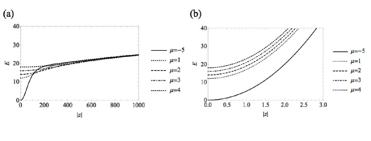
Figure 1: Energy expectations for (a) $\mathrm{CS}(c(4),\mu)$ and (b) $\mathrm{CS}(\tilde{c}(4),\mu),$ for $\mu=-5,1,2,3,4.$

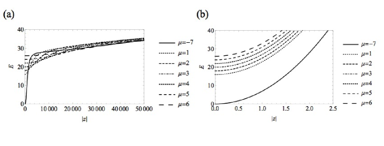
Figure 2: Energy expectations for (a) $\mathrm{CS}(c(6),\mu)$ and (b) $\mathrm{CS}(\tilde{c}(6),\mu),$ for $\mu=-7,1,2,3,4,5,6.$

V Time evolution of position probability densities

We study the time evolution of the position probability densities for the coherent states we have constructed. For the $\mathrm{CS}(c(m),\mu)$ states, we find that for low values of $|z|$ the pattern of many peaks and valleys does not take a simple form. However, in all cases, we find that increasing $|z|$ to very large values gives a pattern of a small number of peaks oscillating in the potential and colliding with each other, producing interference fringes when they collide. We call this regime semi-classical, since it is the closest to the appearance of (more than one) classical particle that we have found.

In our previous paper Hoffmann2018a , we only studied the $\mathrm{CS}(c(2),\mu)$ coherent states to $z=100,$ and did not see the semi-classical regime. Taking $z=17\,000$ for $\mathrm{CS}(c(2),-3)$ (to give the same average energy as $\mathrm{CS}(\tilde{c}(2),-3)$ with $z=15$) shows the semi-classical regime with three wavepackets.

It is now clear that $\mathrm{CS}(c(m),\mu)$ and $\mathrm{CS}(\tilde{c}(m),\mu)$ coherent states show very similar behaviour when compared at the same average energy, but not at the same value of the parameter $z.$

For general $\mathrm{CS}(c(m),\mu),$ the position probability density is given by

$$\rho(x,t;z,m,\mu) =|\langle\,x\,|\,e^{-iH^{-}t}\,|\,z,c,m,\mu\,\rangle|^{2}$$

$$=|\sum_{k=0}^{\infty}\psi_{\mu+(m+1)k}^{(m)}(x)A_{k}^{(m,\mu)}(z\,e^{-i(2m+2)t})|^{2}.$$ (V.1)

For the linearized states $\mathrm{CS}(\tilde{c}(m),\mu)$, the corresponding expression is

$$\tilde{\rho}(x,t;z,m,\mu)=|\sum_{k=0}^{\infty}\psi_{\mu+(m+1)k}^{(m)}(x)\tilde{A}_{k}(z\,e^{-i(2m+2)t})|^{2}.$$ (V.2)

We find that the coefficients $A_{k}^{(m,\mu)}(z)$ fall off very rapidly with $k$ for the values of $z$ we are using. So in practice, we only take the sum in (V.1) to a small cutoff value of $k.$

The state vectors $|\,z,c,m,\mu\,\rangle$ and $|\,\tilde{z},\tilde{c},m,\mu\,\rangle$ have the same average energy and similar behaviour for $|\tilde{z}|$ much less than $|z|,$ as can be seen in Figures 1 and 2. For the $\mathrm{CS}(\tilde{c}(m),\mu)$ states at low $|\tilde{z}|,$ we can also cut off the sums over $k$ at low values.

For $\mathrm{CS}(c(4),-5)$ at $z=100\,000$ and $\mathrm{CS}(\tilde{c}(4),-5)$ at $z=4.7$ (giving the same average energy $\langle\,E\,\rangle=108$) we show the probability densities in Figure 3 and note similar behaviour, both systems being in the semi-classical regime. As noted above, in this regime we see isolated wavepackets oscillating and colliding.

For $m=6$, we display the time-dependence of the position probability density at a set of discrete times. These plots, unlike the 3D plots, do not smear the interference fringes. We note that at times when the wavepackets are well-separated, we count $m+1$ wavepackets, at least for these two choices of $m$ and recalling the result for $m=2$. For $m=6,$ we started with low values of (real, positive) $z$ and found indistinct position probability densities. It was necessary to take $z$ to the extremely large value of $10^{8}$ before the pattern shown below emerged.

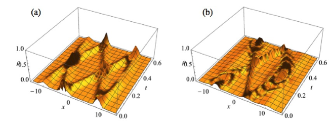
Figure 3: Densities for (a) $\mathrm{CS}(c(4),-5)$ at $z=100\,000$ and (b) $\mathrm{CS}(\tilde{c}(4),-5)$ at $z=4.7.$

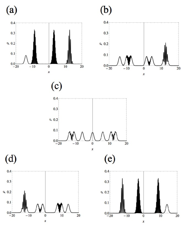
Figure 4: Density for $\mathrm{CS}(c(6),-7)$ at $z=10^{8}$ for (a) $t=0,$ (b) $t=T/8,$ (c) $t=T/4,$ (d) $t=3T/8$ and (e) $t=T/2$ with period $T=\pi/7.$

VI Schrödinger cat states

A cat state is a superposition of two macroscopically distinguishable states. We construct even (+) and odd (-) states by (for $z$ real)

$$|\,z,c,m,\mu,\pm\,\rangle=\frac{1}{\sqrt{2}}\{|\,+z,c,m,\mu\,\rangle\pm|\,-z,c,m,\mu\,\rangle\}.$$ (VI.1)

A measure of the distinguishability of the two component states is (for $m=6$)

$$D(|z|,\mu)=\langle\,+z,c,6,\mu,+\,|\,-z,c,6,\mu\,\rangle=\frac{\phantom{|}{}_{1}F_{7}(1;\frac{\mu+6}{7},\frac{\mu+5}{7},\dots,\frac{\mu+1}{7},\frac{\mu+14}{7};-|z|^{2}/14^{7})}{\phantom{|}{}_{1}F_{7}(1;\frac{\mu+6}{7},\frac{\mu+5}{7},\dots,\frac{\mu+1}{7},\frac{\mu+14}{7};|z|^{2}/14^{7})}.$$ (VI.2)

This is shown in Figure 5, where we see that $z=10^{8}$ is certainly sufficient for distinguishability.

Figure 5: Distinguishability measures for $m=6$ coherent states $\mathrm{CS}(c(6),\mu),$ $\mu=-7,1,2,3,4,5,6.$

The time-dependent position probability densities for these two cat states are shown in a density plot in Figure 6. We see a great deal of structure at this very large value of $z.$ The odd state has a central nodal line, consistent with the parity of the odd wavefunctions.

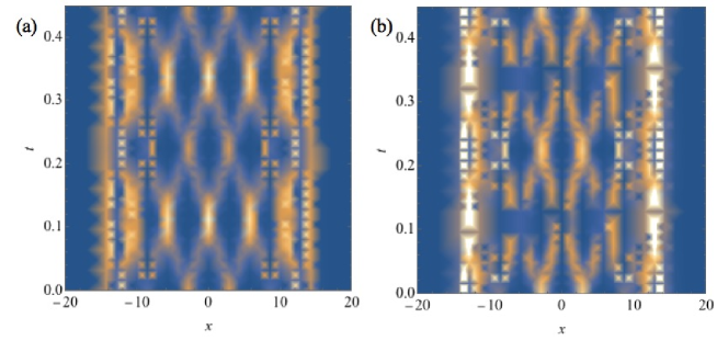
Figure 6: Time-dependent probability densities for (a) even and (b) odd cat states, for $c(6),$ $\mu=-7.$

VII Wigner functions

The Wigner function for a single particle is an everywhere real function of position, $x,$ and momentum, $p,$ so can be considered a distribution in phase space. For the coherent states of the harmonic oscillator, the Wigner functions are everywhere positive Gaussians centred on $x=\mathrm{Re}\,z$ and $p=\mathrm{Im}\,z.$ This fact is used to reinforce the assertion, that we arrived at by looking at the evolution of the position probability density, that the coherent states of the harmonic oscillator are the most closely classical states of a one-dimensional system. It is therefore judged that a state vector does not behave classically, does not have a classical analogue, if its Wigner function is anywhere negative. We will use this criterion to judge the coherent states of our $c(m)$ operators.

For a general state vector $|\,\psi\,\rangle,$ the Wigner function is defined as

$$W(x,p;\psi)=\frac{1}{\pi}\int_{-\infty}^{\infty}dy\,\langle\,\psi\,|\,x-y\,\rangle\langle\,x+y\,|\,\psi\,\rangle e^{-i2py}.$$ (VII.1)

For $|\,\psi\,\rangle=|\,z,c,m,\mu\,\rangle,$we calculate the Wigner function using

$$W(x,p:z,c,m,\mu)=\sum_{k_{1}=0}^{\infty}\sum_{k_{2}=0}^{\infty}A_{k_{1}}^{(m,\mu)*}(z)w_{k_{1}k_{2}}^{(m,\mu)}(x,p)A_{k_{2}}^{(m,\mu)}(z),$$ (VII.2)

with

$$w_{k_{1}k_{2}}^{(m,\mu)}(x,p)=\frac{1}{\pi}\int_{-\infty}^{\infty}dy\,\psi_{\mu+(m+1)k_{1}}^{(m)*}(x-y)\psi_{\mu+(m+1)k_{2}}^{(m)}(x+y)e^{-i2py}.$$ (VII.3)

As we noted in Section V, the coefficients $A_{k}^{(m,\mu)}(z)$ fall off rapidly with $k$ for the small values of $z$ that we consider. We found that it was sufficient to take the sums over $k_{1},k_{2}$ to $k_{1}=k_{2}=10.$

For $m=6$ we found the seven Wigner functions shown in Figure 7. The flat, monotone areas in each graph show where the Wigner function takes on negative values. We conclude that these coherent states do not conform to classical expectations (except for $\mathrm{CS}(c(6),-7)$), as do the harmonic oscillator coherent states.

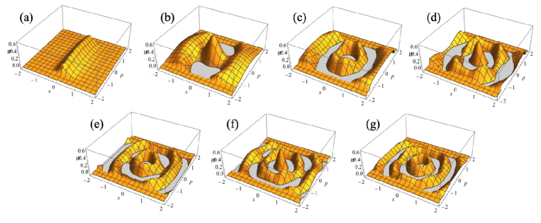
Figure 7: Wigner functions for $\mathrm{CS}(c(6),\mu)$ and $z=10,$ for $\mu$ values (a) -7, (b) 1, (c) 2, (d) 3, (e) 4, (f) 5, (g) 6.

VIII Heisenberg uncertainty relations and squeezing

For our various coherent states, $c(m,\mu)$ and $\tilde{c}(m,\mu),$ we calculate the standard deviations in position and momentum using

$$\sigma_{x} =\sqrt{\langle\,x^{2}\,\rangle-\langle\,x\,\rangle^{2}},$$

$$\sigma_{p} =\sqrt{\langle\,p^{2}\,\rangle-\langle\,p\,\rangle^{2}},$$ (VIII.1)

where the expectation values are in the particular state considered. Then we form the products

$$h(z,m,\mu)=\sigma_{x}(z,m,\mu)\sigma_{p}(z,m,\mu).$$ (VIII.2)

These are required by Heisenberg’s uncertainty principle to be, in all cases, greater than or equal to $1/2.$

The expectation are calculated using, with $|\,\psi\,\rangle=|\,z,c,m,\mu\,\rangle$ again,

$$\langle\,\psi\,|\,\hat{x}\,|\,\psi\,\rangle = \sum_{k_{1}}\sum_{k_{2}}A_{k_{1}}^{(m,\mu)*}(z)M_{k_{1}k_{2}}^{(x)}A_{k_{2}}^{(m,\mu)}(z),$$

$$\langle\,\psi\,|\,\hat{x}^{2}\,|\,\psi\,\rangle = \sum_{k_{1}}\sum_{k_{2}}A_{k_{1}}^{(m,\mu)*}(z)M_{k_{1}k_{2}}^{(x^{2})}A_{k_{2}}^{(m,\mu)}(z),$$

$$\langle\,\psi\,|\,\hat{p}\,|\,\psi\,\rangle = \sum_{k_{1}}\sum_{k_{2}}A_{k_{1}}^{(m,\mu)*}(z)M_{k_{1}k_{2}}^{(p)}A_{k_{2}}^{(m,\mu)}(z),$$

$$\langle\,\psi\,|\,\hat{p}^{2}\,|\,\psi\,\rangle = \sum_{k_{1}}\sum_{k_{2}}A_{k_{1}}^{(m,\mu)*}(z)M_{k_{1}k_{2}}^{(p^{2})}A_{k_{2}}^{(m,\mu)}(z),$$ (VIII.3)

with

$$M_{k_{1}k_{2}}^{(x)} = \int_{-\infty}^{\infty}dx\,\psi_{\mu+(m+1)k_{1}}^{(m)*}(x)\,x\,\psi_{\mu+(m+1)k_{2}}^{(m)}(x),$$

$$M_{k_{1}k_{2}}^{(x^{2})} = \int_{-\infty}^{\infty}dx\,\psi_{\mu+(m+1)k_{1}}^{(m)*}(x)\,x^{2}\psi_{\mu+(m+1)k_{2}}^{(m)}(x),$$

$$M_{k_{1}k_{2}}^{(p)} = \int_{-\infty}^{\infty}dx\,\psi_{\mu+(m+1)k_{1}}^{(m)*}(x)(-i\frac{d}{dx})\psi_{\mu+(m+1)k_{2}}^{(m)}(x),$$

$$M_{k_{1}k_{2}}^{(p^{2})} = \int_{-\infty}^{\infty}dx\,\psi_{\mu+(m+1)k_{1}}^{(m)*}(x)(-\frac{d^{2}}{dx^{2}})\psi_{\mu+(m+1)k_{2}}^{(m)}(x).$$ (VIII.4)

Again the sums over $k_{1},k_{2}$ can be taken to a small finite value depending on the range of $z$ values being considered.

In every case we considered, we found a product $h(z,m,\mu)$ greater than $1/2,$ as expected. In Figure 8 we show the product as a function of $\mathrm{Re}\,z$ and $\mathrm{Im}\,z$ for $\mathrm{CS}(c(4),-5)$ and for $\mathrm{CS}(\tilde{c}(6),-7).$

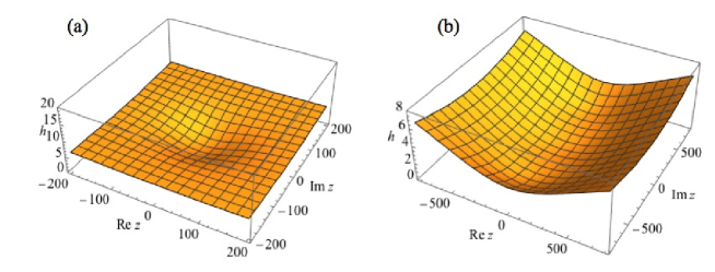
Figure 8: Heisenberg uncertainty relations for (a) $\mathrm{CS}(c(4),-5)$ and (b) $\mathrm{CS}(\tilde{c}(6),-7).$

The Heisenberg uncertainty principle for one-dimensional systems with position and momentum operators, as we have been considering, is $\sigma_{x}\sigma_{p}\geq 1/2.$ This bound is saturated for the coherent states of the harmonic oscillator, where $\sigma_{x}=\sigma_{p}=1/\sqrt{2}$ in our units. It is possible for one of the standard deviations to be less that the harmonic oscillator value, $1/\sqrt{2},$ provided that the other standard deviation is greater than $1/\sqrt{2},$ to preserve the uncertainty relation. In these cases we say that we are dealing with a squeezed state Loudon1987 ; Walls1983 .

We test our coherent states for squeezing and find that it occurs in many cases. For example, Figure 9 shows the observation of squeezing for the $\mathrm{CS}(\tilde{c}(4),-5)$ state in $\sigma_{x}$ at $t=0.$ The graph shows a flat area for $|z|\apprle 0.7$ where $\sigma_{x}$ falls below $1/\sqrt{2}.$

Squeezing has physical applications. Light can be squeezed and used to reduce the noise in measurements Oelker2016 .

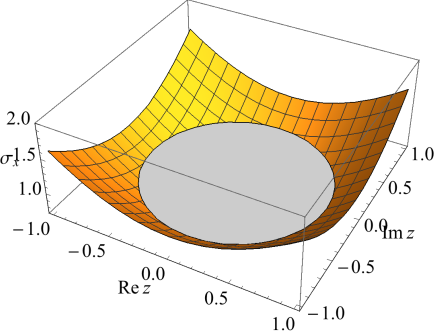
Figure 9: Observation of squeezing for $\mathrm{CS}(\tilde{c}(4),-5)$ (plot of the position standard deviation, $\sigma_{x},$ as a function of $\mathrm{Re}\,z$ and $\mathrm{Im}\,z$).

IX Number statistics

The coherent states of the harmonic oscillator have an excitation number probability distribution (from (III.13))

$$P_{n}(z)=|\langle\,n\,|\,z\,\rangle|^{2}=e^{-|z|^{2}/2}\frac{(|z|^{2}/2)^{n}}{n!},$$ (IX.1)

which is a Poisson distribution with mean number

$$\langle\,N\,\rangle=\frac{|z|^{2}}{2}.$$ (IX.2)

It is easily seen that the number variance satisfies

$$\Delta N^{2}=\langle\,N^{2}\,\rangle-\langle\,N\,\rangle^{2}=\langle\,N\,\rangle.$$ (IX.3)

Then a number distribution with variance less than the average number is called sub-Poissonian, and called super-Poissonian if the variance is greater than the mean. The Mandel $Q$ parameter measures the classification of an arbitrary number distribution:

$$Q=\frac{\Delta N^{2}-\langle\,N\,\rangle}{\langle\,N\,\rangle}=\frac{\langle\,N(N-1)\,\rangle-\langle\,N\,\rangle^{2}}{\langle\,N\,\rangle}.$$ (IX.4)

It vanishes for a Poisson distribution, is negative for a sub-Poissonian distribution and is positive for a super-Poissonian distribution.

We investigate the number statistics of the coherent states labelled $\mathrm{CS}(c(4),\mu)$. We define a number operator, $N_{\mu}$, that acts on the subspace of the order $4$ system with lowest weight $\mu$ by

$$N_{\mu}\,|\,\mu+5k,4\,(-)\,\rangle=k\,|\,\mu+5k,4\,(-)\,\rangle$$ (IX.5)

Then we calculate the Mandel parameter as $Q(c(4),\mu,z)$ where the expectations in (IX.4) are in the state vector $|\,z,c,4,\mu\,\rangle$ and $N=N_{\mu}.$

We find

$$\langle\,N_{\mu}\,\rangle=\frac{1}{(\mu+4)(\mu+3)(\mu+2)(\mu+1)(\mu+10)}\frac{|z|^{2}}{32}\frac{\phantom{|}{}_{1}F_{5}(2;\frac{\mu+9}{5},\frac{\mu+8}{5},\frac{\mu+7}{5},\frac{\mu+6}{5},\frac{\mu+15}{5};|z|^{2}/10^{5})}{\phantom{|}{}_{1}F_{5}(1;\frac{\mu+4}{5},\frac{\mu+3}{5},\frac{\mu+2}{5},\frac{\mu+1}{5},\frac{\mu+10}{5};|z|^{2}/10^{5})}$$ (IX.6)

and

$$\langle\,N_{\mu}(N_{\mu}-1)\,\rangle=\frac{|z|^{4}}{2^{9}}\frac{\phantom{|}{}_{1}F_{5}(3;\frac{\mu+14}{5},\frac{\mu+13}{5},\frac{\mu+12}{5},\frac{\mu+11}{5},\frac{\mu+20}{5};|z|^{2}/10^{5})/\phantom{|}_{1}F_{5}(1;\frac{\mu+4}{5},\frac{\mu+3}{5},\frac{\mu+2}{5},\frac{\mu+1}{5},\frac{\mu+10}{5};|z|^{2}/10^{5})}{(\mu+4)(\mu+3)(\mu+2)(\mu+1)(\mu+10)(\mu+9)(\mu+8)(\mu+7)(\mu+6)(\mu+15)}.$$ (IX.7)

This gives the Mandel $Q$ parameter as a function of $|z|$ for $\mu=-5$ as shown in Figure 10. We see that the parameter is negative except at the origin, indicating sub-Poissonian statistics. This is considered another sign of non-classical behaviour. For other values $\mu=1,2,3,4,$ curves of similar appearance were produced, but with progressively slower variation as $\mu$ was increased.

Figure 10: Mandel $Q$ parameter as a function of $|z|$ for the coherent states $\mathrm{CS}(c(4),-5).$

It should be clear that since the structure of the linearized $\mathrm{CS}(\tilde{c}(m),\mu)$ coherent states is so like that of the harmonic oscillator coherent states, they have only Poisson statistics. To verify this, we find

$$\langle\,N_{\mu}\,\rangle=\sum_{k=0}^{\infty}k\,|\tilde{A}_{k}(z)|^{2}=\sum_{k=0}^{\infty}k\,e^{-|z|^{2}/2}\frac{(|z|^{2}/2)^{k}}{k!}=\frac{|z|^{2}}{2}$$ (IX.8)

and

$$\langle\,N_{\mu}(N_{\mu}-1)\,\rangle=\sum_{k=0}^{\infty}k(k-1)\,|\tilde{A}_{k}(z)|^{2}=\sum_{k=0}^{\infty}k(k-1)\,e^{-|z|^{2}/2}\frac{(|z|^{2}/2)^{k}}{k!}=\left(\frac{|z|^{2}}{2}\right)^{2}.$$ (IX.9)

So

$$Q(\tilde{c}(m),\mu,z)\equiv 0\quad\mathrm{for}\ \mathrm{all}\ m,\mu.$$ (IX.10)

X A coherent state on a beamsplitter

The optical device called a beamsplitter is, in its simplest form, a partially silvered mirror Walls2008 . For a 50:50 beamsplitter (the only case we will consider) half the intensity of a beam of light incident on the beamsplitter is transmitted while the other half is reflected. If two perpendicular beams are incident on the beamsplitter, they are mixed coherently and two perpendicular output beams are produced. If just one incident beam is used, the input in the other direction is the vacuum.

We can place one of our coherent states on one arm of a beamsplitter, with the excitations above the ground state taking the role of photons. We confirm below that if the input is a harmonic oscillator coherent state, representing coherent light, the “photon” number distribution from the two output arms is uncorrelated, factorizing into the product of two independent Poisson number distributions. If a squeezed state is the input, there is correlation and entanglement between the two output arms Sanders2012 ; Ourjoumtsev2009 . Entangled states may have applications in quantum cryptography and quantum teleportation Jennewein2000 ; Bennett1993 . Thus a beamsplitter calculation can give us more information on whether a coherent state displays classical behaviour (like the harmonic oscillator coherent states) or non-classical behaviour.

If $\tilde{c}_{1},\tilde{c}_{1}^{\dagger}$ and $\tilde{c}_{2,}\tilde{c}_{2}^{\dagger}$ are linearized ladder operators for the two input arms (for indices $m$ and $\mu$), respectively, with harmonic oscillator commutation relations, the action of the beamsplitter is represented by the unitary transformation Kim2002

$$U=\exp(i\frac{\pi}{8}(\tilde{c}_{1}\tilde{c}_{2}^{\dagger}+\tilde{c}_{2}\tilde{c}_{1}^{\dagger})),$$ (X.1)

which is seen to give the transformations

$$U\tilde{c}_{1}^{\dagger}U^{\dagger}=\frac{1}{\sqrt{2}}(\tilde{c}_{1}^{\dagger}+i\tilde{c}_{2}^{\dagger}),\quad U\tilde{c}_{2}^{\dagger}U^{\dagger}=\frac{1}{\sqrt{2}}(i\tilde{c}_{1}^{\dagger}+\tilde{c}_{2}^{\dagger}).$$ (X.2)

The factors of $i$ represent $\pi/2$ phase shifts upon reflection. Then it can be shown that

$$U\{|\,n\,\rangle\otimes|\,0\,\rangle\}=\frac{1}{2^{\frac{n}{2}}}\sum_{r=0}^{n}\binom{n}{r}^{\frac{1}{2}}i^{r}|\,n-r\,\rangle\otimes|\,r\,\rangle,$$ (X.3)

where

$$|\,n\,\rangle=|\,\mu+(m+1)n,m\,\rangle.$$ (X.4)

For a general coherent state with coefficients $A_{n}(z),$

$$|\,z\,\rangle=\sum_{n=0}^{\infty}A_{n}(z)\,|\,n\,\rangle,$$ (X.5)

we have the result for the output state

$$|\,\mathrm{out}\,\rangle=U\{|\,z\,\rangle\otimes|\,0\,\rangle\}=\sum_{n=0}^{\infty}\frac{A_{n}(z)}{2^{\frac{n}{2}}}\sum_{r=0}^{n}\binom{n}{r}^{\frac{1}{2}}i^{r}|\,n-r\,\rangle\otimes|\,r\,\rangle.$$ (X.6)

Then the two-photon-number probability distribution for the output arms is

$$P(n_{1},n_{2};z) =|\{\langle\,n_{1}\,|\otimes\langle\,n_{2}\,|\}\,U\{|\,z\,\rangle\otimes|\,0\,\rangle\}|^{2}=\frac{|A_{n_{1}+n_{2}}(z)|^{2}}{2^{n_{1}+n_{2}}}\binom{n_{1}+n_{2}}{n_{2}}.$$ (X.7)

We check for a harmonic oscillator coherent state input,

$$A_{k}^{(0)}(z)=e^{-|z|^{2}/4}(\frac{z}{\sqrt{2}})^{k}\frac{1}{\sqrt{k!}},$$ (X.8)

that

$$P^{(0)}(n_{1},n_{2};z)=p_{n_{1}}(\frac{|z|^{2}}{4})p_{n_{2}}(\frac{|z|^{2}}{4}),$$ (X.9)

where

$$p_{n}(\bar{n})=\frac{e^{-\bar{n}}\bar{n}^{n}}{n!}$$ (X.10)

is the Poisson distribution for mean number $\bar{n}.$ The mean numbers in each arm are half the value for the input state.

For the case $\mathrm{CS}(c(4),-5),$ we found

$$P^{(4,-5)}(n_{1},n_{2};z)=\frac{1}{n_{1}!n_{2}!}\frac{1}{F^{(4,-5)}(z)}\left(\frac{|z|^{2}}{2\times 10^{5}}\right)^{n_{1}+n_{2}}\times\\ \times\frac{\Gamma(-\frac{1}{5})\Gamma(-\frac{2}{5})\Gamma(-\frac{3}{5})\Gamma(-\frac{4}{5})}{\Gamma(n_{1}+n_{2}-\frac{1}{5})\Gamma(n_{1}+n_{2}-\frac{2}{5})\Gamma(n_{1}+n_{2}-\frac{3}{5})\Gamma(n_{1}+n_{2}-\frac{4}{5})}.$$ (X.11)

The presence of functions of $n_{1}+n_{2}$ shows that this probability distribution does not take a factorized form, indicating correlations between the two output arms. We plot this distribution for $z=10^{5}$ and compare this with the harmonic oscillator case for $z=3.5,$ in Figure 11.

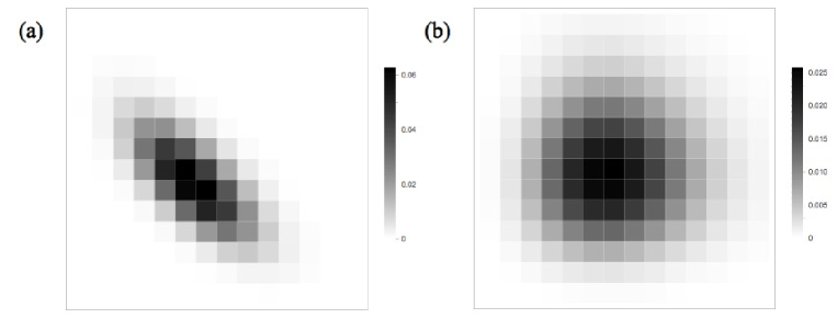
Figure 11: Two-photon-number probability density for (a) the case $\mathrm{CS}(c(4),-5)$ with $z=10^{5}$ and (b) the harmonic oscillator case with $z=3.5$.

It is evident that using the coherent states $\mathrm{CS}(\tilde{c}(m),\mu)$ would give the same result as the harmonic oscillator case.

The linear entropy is widely used as an approximate measure of entanglement in quantum systems, defined by Affleck2009 ; Gerry2009

$$S=1-\mathrm{Tr}\,(\,\rho_{a}^{2}),$$ (X.12)

where the density matrix in our case is (using Eq. (X.6))

$$\rho_{ab}=|\,\mathrm{out}\,\rangle\langle\,\mathrm{out}\,|$$ (X.13)

and

$$\rho_{a}=\sum_{r=0}^{\infty}\langle\,r\,|\,\rho_{ab}\,|\,r\,\rangle$$ (X.14)

is the partial trace of the full density matrix over the quantum number of the second of the systems in the bipartite direct product. The linear entropy can take values in the range $0\leq S<1.$

We find the result for general coherent state coefficients $A_{n}(z)$,

$$S(z)=1-\sum_{r_{1}=0}^{\infty}\sum_{r_{2}=0}^{\infty}\left|\sum_{\kappa=0}^{\infty}G(\kappa+r_{1},r_{1};z)G^{*}(\kappa+r_{2},r_{2};z)\right|^{2},$$ (X.15)

with

$$G(k,r;z)=A_{k}(z)\frac{1}{2^{\frac{k}{2}}}\binom{k}{r}^{\frac{1}{2}}.$$ (X.16)

For a harmonic oscillator coherent state on one input arm of a beamsplitter, the linear entropy of the output state vanishes exactly, consistent with the lack of correlation between the two output arms.

We calculated the linear entropy for the output state of a beamsplitter on which is placed the vacuum and the coherent state labelled $\mathrm{CS}(c(4),-5)$ (the -5 level is the ground state), with coefficients

$$A_{k}^{(4,-5)}(z)=\frac{(-z/10^{\frac{5}{2}})^{k}}{\sqrt{F^{(4,-5)}(z)}}\sqrt{\frac{\Gamma(-\frac{1}{5})\Gamma(-\frac{2}{5})\Gamma(-\frac{3}{5})\Gamma(-\frac{4}{5})}{\Gamma(k-\frac{1}{5})\Gamma(k-\frac{2}{5})\Gamma(k-\frac{3}{5})\Gamma(k-\frac{4}{5})k!}}.$$ (X.17)

in the superposition

$$|\,z,c,4,-5\,\rangle=\sum_{k=0}^{\infty}|\,-5+5k,4\,(-)\,\rangle A_{k}^{(4,-5)}(z),$$ (X.18)

where

$$F^{(4,-5)}(z)=\phantom{|}_{0}F_{4}(-\frac{1}{5},-\frac{2}{5},-\frac{3}{5},-\frac{4}{5};|z|^{2}/10^{5})$$ (X.19)

is a generalized hypergeometric function Gradsteyn1980 .

Figure 12: Linear entropy for the outgoing beamsplitter state for $\mathrm{CS}(c(4),-5)$ as a function of $|z|.$

The results are shown in Figure 12. We see a significantly nonzero linear entropy, indicating entanglement between the two output arms of the beamsplitter. This non-classicality is consistent with what we found from the other measures.

XI Conclusions

We have constructed the $m+1$ orthogonal coherent states, using the Barut-Girardello definition Barut1971 , for the annihilation operator $c(m)$ (obtained by Marquette and Quesne Marquette2013b ; Marquette2013a ), for general $m.$ For comparison, we followed the same procedure for the linearized operators $\tilde{c}(m).$ We calculated the properties of these coherent states, plotting energy expectations, time-dependent position probability densities for the coherent states and for the even and odd cat states, Wigner functions, and Heisenberg uncertainty products. We also plotted the position standard deviations to investigate squeezing and the Mandel $Q$ parameter to investigate number statistics. We placed one of our coherent states on one arm of a beamsplitter and calculated the two “photon” number probability distribution for the output arms. Then we calculated the linear entropy for an example output state.

We found that the position probability density for a $c(m)$ coherent state is rather indistinct for low values of $|z|,$ but for sufficiently large values it separates into $m+1$ distinct wavepackets, oscillating in the potential and colliding to produce interference fringes. We saw the same behaviour for the $\tilde{c}(m)$ coherent states, at much lower values of $|z|,$ but at comparable average energies. Consequently, the even and odd cat states display a great deal of wavepacket structure.

We found the Wigner function to take on negative values for all but the case $\mu=-7$ of $m=6,$ an indication of non-classical behaviour. The Heisenberg uncertainty products for two cases showed minima at $z=0$ with minimum values greater than $1/2.$ By plotting the standard deviation in position for our coherent states as a function of $\mathrm{Re}\,z$ and $\mathrm{Im}\,z$, and finding where it fell below $1/\sqrt{2},$ we were able to observe squeezing in many of our cases.

The Mandel $Q$ parameter was found to be negative in all cases of $m=4$ (except at $z=0,$ where it vanished) indicating sub-Poissonian statistics and, again, non-classical behaviour.

We found correlations in the output arms two-number distribution (it did not factorize) for one of our coherent states on a beamsplitter, another indication of non-classical behaviour. The linear entropy was calculated for the beamsplitter output state and was found to take significant nonzero values (except for $z=0$), indicating the presence of entanglement, another non-classical feature.

- (1) Hoffmann SE, Hussin V, Marquette I, Zhang YZ. Non-classical behaviour of coherent states for systems constructed using exceptional orthogonal polynomials. J Phys A: Math Theor. 2018;51(8):085202.
- (2) Marquette I, Quesne C. New ladder operators for a rational extension of the harmonic oscillator and superintegrability of some two-dimensional systems. J Math Phys. 2013;54(10):102102.
- (3) Marquette I, Quesne C. Two-step rational extensions of the harmonic oscillator: exceptional orthogonal polynomials and ladder operators. J Phys A: Math Theor. 2013;46(15):155201.
- (4) Gómez-Ullate D, Kamran N, Milson R. An extension of Bochner’s problem: Exceptional invariant subspaces. J Approx Th. 2010;162(5):987 – 1006.
- (5) Glauber RJ. The quantum theory of optical coherence. Phys Rev. 1963;130:2529.
- (6) Glauber RJ. Coherent and incoherent states of the radiation field. Phys Rev. 1963;131:2766.
- (7) Klauder JR. Continuous representation theory. I. Postulates of continuous representation theory. J Math Phys. 1963;4(8):1055.
- (8) Klauder JR. Continuous representation theory. II. Generalized relation between quantum and classical dynamics. J Math Phys. 1963;4(8):1058.
- (9) Barut AO, Girardello L. New ”coherent” states associated with non compact groups. Commun Math Phys. 1971;21:41.
- (10) Perelomov A. Generalized coherent states and their applications. Springer-Verlag, Berlin, Heidelberg; 1986.
- (11) Gazeau JP, Klauder JR. Coherent states for systems with discrete and continuous spectrum. J Phys A: Math Gen. 1999;32(1):123.
- (12) Quesne C. Generalized coherent states associated with the Cv-extended oscillator. Ann Phys (NY). 2001;293:147.
- (13) Fernández DJ, Nieto LM, Rosas-Ortiz O. Distorted Heisenberg algebra and coherent states for isospectral oscillator Hamiltonians. J Phys A: Math Gen. 1995;28(9):2693.
- (14) Fernández DJ, Hussin V. Higher-order SUSY, linearized nonlinear Heisenberg algebras and coherent states. J Phys A: Math Gen. 1999;32(19):3603.
- (15) D Gómez-Ullate YG, Milson R. Rational extensions of the quantum harmonic oscillator and exceptional Hermite polynomials. J Phys A: Math Theor. 2014;47:015203.
- (16) Ali ST, Antoine JP, Gazeau JP. Coherent states, wavelets and their generalizations. 2nd ed. Springer-Verlag, New York; 2014.
- (17) Bermudez D, Contreras-Astorga A, Fernández DJ. Painlevé IV Hamiltonian systems and coherent states. J Phys: Conf Ser. 2015;597(1):012017.
- (18) Gradsteyn IS, Ryzhik IM. Tables of Integrals, Series and Products. Corrected and enlarged ed. Academic Press, Inc., San Diego, CA; 1980.
- (19) Fernández DJ, Hussin V, Nieto LM. Coherent states for isospectral oscillator Hamiltonians. J Phys A: Math Gen. 1994;27(10):3547.
- (20) Loudon R, Knight PL. Squeezed Light. Journal of Modern Optics. 1987;34(6-7):709–759.
- (21) Walls DF. Squeezed states of light. Nature. 1983;306:141 EP –.
- (22) Oelker E, et al. Ultra-low phase noise squeezed vacuum source for gravitational wave detectors. Optica. 2016;3(7):682.
- (23) Walls DF, Milburn GJ. Quantum Optics. Springer, Berlin; 2008.
- (24) Sanders BC. Review of entangled coherent states. J Phys A: Math Theor. 2012;45(24):244002.
- (25) Ourjoumtsev A, Ferreyrol F, Tualle-Brouri R, Grangier P. Preparation of non-local superpositions of quasi-classical light states. Nat Phys. 2009 02;5:189.
- (26) Jennewein T, Simon C, Weihs G, Weinfurter H, Zeilinger A. Quantum Cryptography with Entangled Photons. Phys Rev Lett. 2000;84:4729–4732.
- (27) Bennett CH, Brassard G, Crépeau C, Jozsa R, Peres A, Wootters WK. Teleporting an unknown quantum state via dual classical and Einstein-Podolsky-Rosen channels. Phys Rev Lett. 1993;70:1895–1899.
- (28) Kim MS, Son W, Bužek V, Knight PL. Entanglement by a beam splitter: Nonclassicality as a prerequisite for entanglement. Phys Rev A. 2002;65(3).
- (29) Affleck I, Laflorencie N, Sørensen ES. Entanglement entropy in quantum impurity systems and systems with boundaries. Journal of Physics A: Mathematical and Theoretical. 2009;42(50):504009.
- (30) Gerry CC, Benmoussa A. Beam splitting and entanglement: Generalized coherent states, group contraction, and the classical limit. Phys Rev A. 2005;71:062319.