Thermodynamics in $f(\mathcal{G},T)$ Gravity

Abstract

This paper explores the non-equilibrium behavior of thermodynamics at the apparent horizon of isotropic and homogeneous universe model in $f(\mathcal{G},T)$ gravity ($\mathcal{G}$ and $T$ represent the Gauss-Bonnet invariant and trace of the energy-momentum tensor, respectively). We construct the corresponding field equations and analyze the first as well as generalized second law of thermodynamics in this scenario. It is found that an auxiliary term corresponding to entropy production appears due to the non-equilibrium picture of thermodynamics in first law. The universal condition for the validity of generalized second law of thermodynamics is also obtained. Finally, we check the validity of generalized second law of thermodynamics for the reconstructed $f(\mathcal{G},T)$ models (de Sitter and power-law solutions). We conclude that this law holds for suitable choices of free parameters.

Keywords: Modified gravity; Thermodynamics.
PACS: 04.50.Kd; 05.70.-a.

1 Introduction

The discovery of current cosmic accelerated expansion has stimulated many researchers to explore the cause of this tremendous change in cosmic history. A mysterious force known as dark energy (DE) is considered as the basic ingredient responsible for this expanding phase of the universe. Dark energy has repulsive nature with negatively large pressure but its complete characteristics are still unknown. Modified gravity theories are considered as the favorable and optimistic approaches to unveil the salient features of DE. These modified theories of gravity are obtained by replacing or adding curvature invariants as well as their corresponding generic functions in the Einstein-Hilbert action.

Gauss-Bonnet (GB) invariant is a linear combination of quadratic invariants of the form

$$\mathcal{G}=R^{2}-4R_{\mu\nu}R^{\mu\nu}+R_{\mu\nu\xi\eta}R^{\mu\nu\xi\eta},$$

where $R,~{}R_{\mu\nu}$ and $R_{\mu\nu\xi\eta}$ denote the Ricci scalar, Ricci and Riemann tensors, respectively. It is the second order Lovelock scalar with the interesting feature that it is free from spin-2 ghost instabilities while its dynamical effects do not appear in four dimensions [1]. The coupling of $\mathcal{G}$ with scalar field or adding generic function $f(\mathcal{G})$ in geometric part of the Einstein-Hilbert action are the two promising ways to study the dynamics of $\mathcal{G}$ in four dimensions. Nojiri and Odintsov [2] presented the second approach as an alternative for DE referred as $f(\mathcal{G})$ gravity which explores the fascinating characteristics of late-time cosmological evolution. This theory is consistent with solar system constraints and has a quite rich cosmological structure [3].

The curvature-matter coupling in modified theories has attained much attention to discuss the cosmic accelerated expansion. Harko et al. [4] introduced such coupling in $f(R)$ gravity referred as $f(R,T)$ gravity. Recently, we have established this coupling between quadratic curvature invariant and matter named as $f(\mathcal{G},T)$ theory of gravity and found that such coupling leads to the non-conservation of energy-momentum tensor $(T_{\mu\nu})$ [5]. Furthermore, the non-geodesic lines of geometry are followed by massive test particles due to the presence of extra force while dust particles follow geodesic trajectories. The stability of Einstein universe is analyzed for both conserved as well as non-conserved $T_{\mu\nu}$ in this theory [6]. Shamir and Ahmad [7] applied Noether symmetry approach to construct some cosmological viable $f(\mathcal{G},T)$ models in the background of isotropic and homogeneous universe. We have reconstructed the cosmic evolutionary models corresponding to phantom/non-phantom epochs, de Sitter universe as well as power-law solution and analyzed their stability [8].

The significant connection between gravitation and thermodynamics is established after the remarkable discovery of black hole (BH) thermodynamics with Hawking temperature as well as BH entropy [9]. Jacobson [10] obtained the Einstein field equations using fundamental relation known as Clausius relation $dQ=\mathcal{T}d\mathcal{S}$ ($\mathcal{S},~{}\mathcal{T}$ and $dQ$ represent the entropy, Unruh temperature and energy flux observed by accelerated observer just inside the horizon, respectively) together with the proportionality of entropy and horizon area in the context of Rindler spacetime. Cai and Kim [11] showed that Einstein field equations can be rewritten in the form of first law of thermodynamics for isotropic and homogeneous universe with any spatial curvature parameter. Akbar and Cai [12] found that the Friedmann equations at the apparent horizon can be written in the form $dE=\mathcal{T}d\mathcal{S}+Wd\mathcal{V}$ ($E,~{}\mathcal{V}$ and $W$ are the energy, volume inside the horizon and work density, respectively) in general relativity (GR), GB gravity and the general Lovelock theory of gravity. In modified theories, an additional entropy production term is appeared in Clausius relation that corresponds to the non-equilibrium behavior of thermodynamics while no extra term appears in GB gravity, Lovelock gravity and braneworld gravity [13].

The generalized second law of thermodynamics (GSLT) has a significant importance in modified theories of gravity. Wu et al. [14] derived the universal condition for the validity of GSLT in modified theories of gravity. Bamba and Geng [15] found that GSLT in the effective phantom/non-phantom phase is satisfied in $f(R)$ gravity. Sadjadi [16] studied the second law as well as GSLT in $f(R,\mathcal{G})$ gravity for de Sitter universe model as well as power-law solution with the assumption that apparent horizon is in thermal equilibrium. Bamba and Geng [17] found that GSLT holds for the FRW universe with the same temperature inside and outside the apparent horizon in generalized teleparallel theory. Sharif and Zubair [18] checked the validity of first and second laws of thermodynamics at the apparent horizon for both equilibrium as well as non-equilibrium descriptions in $f(R,T)$ gravity and found that GSLT holds in both phantom as well as non-phantom phases of the universe. Abdolmaleki and Najafi [19] explored the validity of GSLT for isotropic and homogeneous universe filled with radiation and matter surrounded by apparent horizon with Hawking temperature in $f(\mathcal{G})$ gravity.

In this paper, we investigate the first as well as second law of thermodynamics at the apparent horizon of FRW model with any spatial curvature. The paper has the following format. In section 2, we discuss the basic formalism of this gravity while the laws of thermodynamics are investigated in section 3. Section 4 is devoted to analyze the validity of GSLT for reconstructed $f(\mathcal{G},T)$ models corresponding to de Sitter and power-law solution. The results are summarized in the last section.

2 $f(\mathcal{G},T)$ Gravity

The action of $f(\mathcal{G},T)$ gravity is given by [5]

$$\mathcal{I}=\int\sqrt{-g}\left(\frac{R+f(\mathcal{G},T)}{16\pi G}+\mathcal{L}_{m}\right)d^{4}x,$$ (1)

where $g,~{}G$ and $\mathcal{L}_{m}$ represent determinant of the metric tensor $(g_{\mu\nu})$, gravitational constant and matter Lagrangian density, respectively. The variation of the action (1) with respect to $g_{\mu\nu}$ gives the fourth-order field equations as

$$R_{\mu\nu}-\frac{1}{2}g_{\mu\nu}R = \frac{1}{2}g_{\mu\nu}f(\mathcal{G},T)-2RR_{\mu\nu}f_{\mathcal{G}}(\mathcal{G},T)+4R^{\xi}_{\mu}R_{\xi\nu}f_{\mathcal{G}}(\mathcal{G},T)$$ (2)

$$+ 4R_{\mu\xi\nu\eta}R^{\xi\eta}f_{\mathcal{G}}(\mathcal{G},T)-2R_{\mu}^{\xi\eta\delta}R_{\nu\xi\eta\delta}f_{\mathcal{G}}(\mathcal{G},T)-2Rg_{\mu\nu}$$

$$\times \nabla^{2}f_{\mathcal{G}}(\mathcal{G},T)+4R_{\mu\nu}\nabla^{2}f_{\mathcal{G}}(\mathcal{G},T)+2R\nabla_{\mu}\nabla_{\nu}f_{\mathcal{G}}(\mathcal{G},T)$$

$$- 4R^{\xi}_{\nu}\nabla_{\mu}\nabla_{\xi}f_{\mathcal{G}}(\mathcal{G},T)-4R^{\xi}_{\mu}\nabla_{\nu}\nabla_{\xi}f_{\mathcal{G}}(\mathcal{G},T)+4g_{\mu\nu}R^{\xi\eta}$$

$$\times \nabla_{\xi}\nabla_{\eta}f_{\mathcal{G}}(\mathcal{G},T)-4R_{\mu\xi\nu\eta}\nabla^{\xi}\nabla^{\eta}f_{\mathcal{G}}(\mathcal{G},T)-(T_{\mu\nu}+\Theta_{\mu\nu})$$

$$\times f_{T}(\mathcal{G},T)+8\pi GT_{\mu\nu},$$

where $f_{\mathcal{G}}(\mathcal{G},T)=\frac{\partial f(\mathcal{G},T)}{\partial\mathcal{G}},~{}f_{T}(\mathcal{G},T)=\frac{\partial f(\mathcal{G},T)}{\partial T},~{}\nabla^{2}=\nabla_{\mu}\nabla^{\mu}$ ($\nabla_{\mu}$ is a covariant derivative) and $\Theta_{\mu\nu}$ has the following expression [20]

$$\Theta_{\mu\nu}=-2T_{\mu\nu}+g_{\mu\nu}\mathcal{L}_{m}-2g^{\xi\eta}\frac{\partial^{2}\mathcal{L}_{m}}{\partial g^{\mu\nu}\partial g^{\xi\eta}}.$$

The variation of $\sqrt{-g}\mathcal{L}_{m}$ with respect to $g_{\mu\nu}$ yields

$$T_{\mu\nu}=g_{\mu\nu}\mathcal{L}_{m}-2\frac{\partial\mathcal{L}_{m}}{\partial g^{\mu\nu}},$$

where we have used that $\mathcal{L}_{m}$ depends only on $g_{\mu\nu}$.

The covariant derivative of Eq.(2) gives

$$\nabla^{\mu}T_{\mu\nu} = -\frac{f_{T}(\mathcal{G},T)}{8\pi G-f_{T}(\mathcal{G},T)}\left[\frac{1}{2}g_{\mu\nu}\nabla^{\mu}T-(\Theta_{\mu\nu}+T_{\mu\nu})\nabla^{\mu}\ln f_{T}(\mathcal{G},T)\right.$$ (3)

$$- \left.\nabla^{\mu}\Theta_{\mu\nu}\right].$$

The non-zero divergence shows that the conservation law does not hold in this gravity due to the curvature-matter coupling. The above equations show that matter Lagrangian density and a generic function have a significant importance to discuss the dynamics of curvature-matter coupled theories. The particular forms of $f(\mathcal{G},T)$ are

$$f(\mathcal{G},T)=f_{1}(\mathcal{G})+f_{2}(T),\quad f(\mathcal{G},T)=f_{1}(\mathcal{G})+f_{2}(\mathcal{G})f_{3}(T),$$

where the first choice is considered as correction to $f(\mathcal{G})$ gravity since it does not involve the direct non-minimal curvature-matter coupling while the second form implies direct coupling. Unlike $f(R,T)$ gravity [4], the choice $f(\mathcal{G},T)=\mathcal{G}+\lambda T$ ($\lambda$ is an arbitrary parameter) does not exist in this gravity since $\mathcal{G}$ is a topological invariant in four dimensions. It is clear from Eq.(2) that the contribution of GB disappears for this particular choice of the model.

The energy-momentum tensor for perfect fluid as cosmic matter contents is given by

$$T_{\mu\nu}=(\rho+P)v_{\mu}v_{\nu}-Pg_{\mu\nu},$$ (4)

where $P,~{}\rho$ and $v_{\mu}$ denote pressure, energy density and four-velocity, respectively. This four-velocity satisfies the relations $v^{\xi}v_{\xi}=1$ and $v^{\xi}\nabla_{\nu}v_{\xi}=0$. In this case, the tensor $\Theta_{\mu\nu}$ with $\mathcal{L}_{m}=-P$ takes the form

$$\Theta_{\mu\nu}=-Pg_{\mu\nu}-2T_{\mu\nu}.$$ (5)

Using Eqs.(4) and (5), Eq.(2) can be written in a similar form as the Einstein field equations for dust case $(P=0)$

$$G_{\mu\nu}=8\pi\widetilde{G}T_{\mu\nu}^{\mathrm{eff}}=8\pi\widetilde{G}T_{\mu\nu}+T_{\mu\nu}^{\mathrm{(D)}},$$ (6)

where

$$T_{\mu\nu}^{\mathrm{(D)}} = \frac{1}{2}g_{\mu\nu}f(\mathcal{G},T)-2RR_{\mu\nu}f_{\mathcal{G}}(\mathcal{G},T)+4R^{\xi}_{\mu}R_{\xi\nu}f_{\mathcal{G}}(\mathcal{G},T)$$

$$+ 4R_{\mu\xi\nu\eta}R^{\xi\eta}f_{\mathcal{G}}(\mathcal{G},T)-2R_{\mu}^{\xi\eta\delta}R_{\nu\xi\eta\delta}f_{\mathcal{G}}(\mathcal{G},T)-2Rg_{\mu\nu}\nabla^{2}f_{\mathcal{G}}(\mathcal{G},T)$$

$$+ 4R_{\mu\nu}\nabla^{2}f_{\mathcal{G}}(\mathcal{G},T)+2R\nabla_{\mu}\nabla_{\nu}f_{\mathcal{G}}(\mathcal{G},T)-4R^{\xi}_{\nu}\nabla_{\mu}\nabla_{\xi}f_{\mathcal{G}}(\mathcal{G},T)$$

$$- 4R^{\xi}_{\mu}\nabla_{\nu}\nabla_{\xi}f_{\mathcal{G}}(\mathcal{G},T)+4g_{\mu\nu}R^{\xi\eta}\nabla_{\xi}\nabla_{\eta}f_{\mathcal{G}}(\mathcal{G},T)$$

$$- 4R_{\mu\xi\nu\eta}\nabla^{\xi}\nabla^{\eta}f_{\mathcal{G}}(\mathcal{G},T),$$

$$\widetilde{G} = GF,\quad F=1+\frac{f_{T}(\mathcal{G},T)}{8\pi G}.$$

The line element for FRW universe model is

$$ds^{2}=dt^{2}-\frac{a^{2}(t)}{1-kr^{2}}dr^{2}-\hat{r}^{2}d\theta^{2}-\hat{r}^{2}\sin^{2}\theta d\phi^{2},$$ (7)

where $\hat{r}=a(t)r,~{}a(t)$ and $k$ represent the scale factor depending on cosmic time and spatial curvature parameter which corresponds to open $(k=-1)$, closed $(k=1)$ and flat $(k=0)$ geometries of the universe. The GB invariant takes the form

$$\mathcal{G}=24(H^{2}+\dot{H})\left(H^{2}+\frac{k}{a^{2}}\right).$$

Using Eqs.(4), (6) and (7), we obtain the following field equations

$$3\left(H^{2}+\frac{k}{a^{2}}\right) = 8\pi\widetilde{G}\rho+\frac{1}{2}f(\mathcal{G},T)-12(H^{2}+\dot{H})\left(H^{2}+\frac{k}{a^{2}}\right)$$ (8)

$$\times f_{\mathcal{G}}(\mathcal{G},T)+12H\left(H^{2}+\frac{k}{a^{2}}\right)\left(f_{\mathcal{GG}}(\mathcal{G},T)\dot{\mathcal{G}}\right.$$

$$+ \left.f_{\mathcal{G}T}(\mathcal{G},T)\dot{T}\right),$$

$$-\left(2\dot{H}+3H^{2}+\frac{k}{a^{2}}\right) = -\frac{1}{2}f(\mathcal{G},T)+12(H^{2}+\dot{H})\left(H^{2}+\frac{k}{a^{2}}\right)f_{\mathcal{G}}(\mathcal{G},T)$$ (9)

$$- 8H(H^{2}+\dot{H})\left(f_{\mathcal{GG}}(\mathcal{G},T)\dot{\mathcal{G}}+f_{\mathcal{G}T}(\mathcal{G},T)\dot{T}\right)$$

$$- 4\left(H^{2}+\frac{k}{a^{2}}\right)\left(f_{\mathcal{GGG}}(\mathcal{G},T)\dot{\mathcal{G}}^{2}+2f_{\mathcal{GG}T}(\mathcal{G},T)\dot{\mathcal{G}}\dot{T}\right.$$

$$+ \left.f_{\mathcal{G}TT}(\mathcal{G},T)\dot{T}^{2}+f_{\mathcal{GG}}(\mathcal{G},T)\ddot{\mathcal{G}}+f_{\mathcal{G}T}(\mathcal{G},T)\ddot{T}\right),$$

where $H=\dot{a}/a$ is a Hubble parameter and dot represents derivative with respect to time. We can rewrite the above equations as

$$3\left(H^{2}+\frac{k}{a^{2}}\right) = 8\pi\widetilde{G}\rho_{\mathrm{{}_{tot}}}=8\pi\widetilde{G}(\rho+\rho^{\mathrm{(D)}}),$$ (10)

$$-2\left(\dot{H}-\frac{k}{a^{2}}\right) = 8\pi\widetilde{G}(\rho_{\mathrm{{}_{tot}}}+P_{\mathrm{{}_{tot}}})=8\pi\widetilde{G}(\rho+\rho^{\mathrm{(D)}}+P^{\mathrm{(D)}}),$$ (11)

where $\rho_{\mathrm{(D)}}$ and $P_{\mathrm{(D)}}$ are dark source terms given by

$$\rho^{\mathrm{(D)}} = \frac{1}{8\pi\widetilde{G}F}\left[\frac{1}{2}f(\mathcal{G},T)-12(H^{2}+\dot{H})\left(H^{2}+\frac{k}{a^{2}}\right)f_{\mathcal{G}}(\mathcal{G},T)\right.$$

$$+ \left.12H\left(H^{2}+\frac{k}{a^{2}}\right)\left(f_{\mathcal{GG}}(\mathcal{G},T)\dot{\mathcal{G}}+f_{\mathcal{G}T}(\mathcal{G},T)\dot{T}\right)\right],$$

$$P^{\mathrm{(D)}} = \frac{1}{8\pi\widetilde{G}F}\left[-\frac{1}{2}f(\mathcal{G},T)+12(H^{2}+\dot{H})\left(H^{2}+\frac{k}{a^{2}}\right)f_{\mathcal{G}}(\mathcal{G},T)-8H\right.$$

$$\times \left.(H^{2}+\dot{H})\left(f_{\mathcal{GG}}(\mathcal{G},T)\dot{\mathcal{G}}+f_{\mathcal{G}T}(\mathcal{G},T)\dot{T}\right)-4\left(H^{2}+\frac{k}{a^{2}}\right)\right.$$

$$\times \left.\left(f_{\mathcal{GGG}}(\mathcal{G},T)\dot{\mathcal{G}}^{2}+2f_{\mathcal{GG}T}(\mathcal{G},T)\dot{\mathcal{G}}\dot{T}+f_{\mathcal{G}TT}(\mathcal{G},T)\dot{T}^{2}+f_{\mathcal{GG}}(\mathcal{G},T)\ddot{\mathcal{G}}\right.\right.$$

$$+ \left.\left.f_{\mathcal{G}T}(\mathcal{G},T)\ddot{T}\right)\right].$$

The continuity equation for Eq.(7) becomes

$$\dot{\rho}+3H\rho=\frac{-1}{8\pi G+f_{T}(\mathcal{G},T)}\left[\frac{1}{2}\dot{\rho}f_{T}(\mathcal{G},T)+\rho\left(f_{\mathcal{G}T}(\mathcal{G},T)\dot{\mathcal{G}}+f_{TT}(\mathcal{G},T)\dot{T}\right)\right].$$ (12)

The conservation law holds in the absence of curvature-matter coupling for both $f(\mathcal{G})$ gravity and GR.

3 Laws of Thermodynamics

In this section, we study the laws of thermodynamics in the context of $f(\mathcal{G},T)$ gravity at the apparent horizon of FRW universe model.

3.1 First Law

The first law of thermodynamics is based on the concept that energy remains conserved in the system but can change from one form to another. To study this law, we first find the dynamical apparent horizon evaluated by the relation

$$h^{\mu\nu}\partial_{\mu}\hat{r}\partial_{\nu}\hat{r}=0,$$

where $h_{\mu\nu}=\mathrm{diag}(1,\frac{-a^{2}}{1-kr^{2}})$ is a two-dimensional metric. For isotropic and homogeneous universe model, the above relation gives the radius of apparent horizon as

$$\hat{r}_{A}=\left(H^{2}+\frac{k}{a^{2}}\right)^{-\frac{1}{2}}.$$

Taking the time derivative of this equation and using Eq.(11), it follows that

$$d\hat{r}_{A}=4\pi G\left(\rho_{\mathrm{{}_{tot}}}+P_{\mathrm{{}_{tot}}}\right)\hat{r}_{A}^{3}HFdt,$$ (13)

where $d{\hat{r}_{A}}$ represents the infinitesimal change in apparent horizon radius during the small time interval $dt$.

Bekenstein-Hawking entropy is defined as one fourth of apparent horizon area $(\mathcal{A}=4\pi\hat{r}_{A}^{2})$ in units of Newton’s gravitational constant [9]. In modified theories of gravity, the entropy of stationary BH solutions with bifurcate Killing horizons is a Noether charge entropy also known as Wald entropy [21]. It depends on the variation of Lagrangian density $(\mathcal{L})$ with respect to $R_{\mu\nu\xi\eta}$ as [22]

$$\mathcal{S}=-2\pi\oint\frac{\partial\mathcal{L}}{\partial R_{\mu\nu\xi\eta}}\epsilon_{\xi\eta}\epsilon_{\mu\nu}dV_{n-2}^{2},$$ (14)

where $dV_{n-2}^{2}$ and $\epsilon_{\xi\eta}$ represent the volume element on $(n-2)$-dimensional spacelike bifurcation surface $(\Sigma)$ and binormal vector to $\Sigma$ satisfying the relation $\epsilon_{\xi\eta}\epsilon^{\xi\eta}=-2$. Brustein et al. [23] proposed that Wald entropy is equal to quarter of $\mathcal{A}$ in units of the effective gravitational coupling in modified theories of gravity. Using these concepts, the Wald entropy in $f(\mathcal{G},T)$ gravity is given by

$$\mathcal{S}=\frac{\mathcal{A}}{4GF}\left(1-\frac{4}{\hat{r}_{A}^{2}}f_{\mathcal{G}}(\mathcal{G},T)\right).$$ (15)

This formula corresponds to $f(\mathcal{G})$ gravity for $F=1$ while the traditional entropy in GR is obtained for $f_{\mathcal{G}}=0$ [24]. Taking differential of Eq.(15) and using Eq.(13), we obtain

$$\frac{1}{2\pi\hat{r}_{A}}d\mathcal{S}=4\pi\left(\rho_{\mathrm{{}_{tot}}}+P_{\mathrm{{}_{tot}}}\right)\hat{r}_{A}^{3}Hdt-\frac{2}{\hat{r}_{A}GF}df_{\mathcal{G}}+\frac{\hat{r}_{A}}{2G}\left(1-\frac{4}{\hat{r}_{A}^{2}}\ f_{\mathcal{G}}\right)d\left(\frac{1}{F}\right).$$ (16)

The surface gravity $(\kappa_{sg})$ helps to determine temperature on the apparent horizon as [11]

$$\mathcal{T}=\frac{|\kappa_{sg}|}{2\pi},$$ (17)

where

$$\kappa_{sg} = \frac{1}{2\sqrt{-h}}\partial_{\mu}\left(\sqrt{-h}h^{\mu\nu}\partial_{\nu}\hat{r}\right)$$ (18)

$$= \frac{1}{\hat{r}_{A}}\left(1-\frac{\dot{\hat{r}}_{A}}{2\hat{r}_{A}H}\right)=\frac{1}{2}\hat{r}_{A}\left(\frac{k}{a^{2}}+H^{2}+\dot{H}\right),$$

$h$ is the determinant of $h_{\mu\nu}$. Using Eqs.(16)-(18), we have

$$\mathcal{T}d\mathcal{S} = 4\pi\left(\rho_{\mathrm{{}_{tot}}}+P_{\mathrm{{}_{tot}}}\right)\hat{r}_{A}^{3}Hdt-2\pi\left(\rho_{\mathrm{{}_{tot}}}+P_{\mathrm{{}_{tot}}}\right)\hat{r}_{A}^{2}d\hat{r}_{A}-\frac{4\pi\mathcal{T}}{GF}df_{\mathcal{G}}$$ (19)

$$+ \frac{\pi}{G}\hat{r}_{A}^{2}\mathcal{T}\left(1-\frac{4}{\hat{r}_{A}^{2}}f_{\mathcal{G}}\right)d\left(\frac{1}{F}\right).$$

The total energy inside the apparent horizon of radius $\hat{r}_{A}$ for FRW universe model is given by

$$E=\mathcal{V}\rho_{\mathrm{{}_{tot}}}=\frac{4}{3}\pi\hat{r}_{A}^{3}\rho_{\mathrm{{}_{tot}}}=\frac{3\mathcal{V}}{8\pi\widetilde{G}}\left(H^{2}+\frac{k}{a^{2}}\right).$$

This equation shows that $E$ is directly related to $\hat{r}_{A}$, so the small displacement $d\hat{r}_{A}$ in horizon radius will cause the infinitesimal change given by

$$dE=4\pi\rho_{\mathrm{{}_{tot}}}\hat{r}_{A}^{2}d\hat{r}_{A}-4\pi\left(\rho_{\mathrm{{}_{tot}}}+P_{\mathrm{{}_{tot}}}\right)\hat{r}_{A}^{3}Hdt+\frac{\hat{r}_{A}}{2G}d\left(\frac{1}{F}\right).$$ (20)

Using Eqs.(19) and (20), it follows that

$$\mathcal{T}d\mathcal{S}=-dE+Wd\mathcal{V}-\frac{4\pi\mathcal{T}}{GF}df_{\mathcal{G}}+\frac{\hat{r}_{A}}{2G}\left[1+2\pi\hat{r}_{A}\mathcal{T}\left(1-\frac{4}{\hat{r}_{A}^{2}}f_{\mathcal{G}}\right)\right]d\left(\frac{1}{F}\right),$$

where $W=\left(\rho_{\mathrm{{}_{tot}}}-P_{\mathrm{{}_{tot}}}\right)/2$ is the work done by the system. The above equation can be written as

$$\mathcal{T}\left(d\mathcal{S}+d_{i}\mathcal{S}\right)=-dE+Wd\mathcal{V},$$ (21)

where

$$d_{i}\mathcal{S}=\frac{4\pi}{GF}df_{\mathcal{G}}-\frac{\hat{r}_{A}}{2G\mathcal{T}}\left[1+2\pi\hat{r}_{A}\mathcal{T}\left(1-\frac{4}{\hat{r}_{A}^{2}}f_{\mathcal{G}}\right)\right]d\left(\frac{1}{F}\right),$$

is interpreted as the entropy production term which appears due to non-equilibrium thermodynamical behavior at the apparent horizon. The non-equilibrium picture of thermodynamics implies that there is some energy change inside and outside the apparent horizon. Due to the presence of this extra term, the field equations do not obey the universal form of first law of thermodynamics $dE=\mathcal{T}d\mathcal{S}+Wd\mathcal{V}$ in this gravity. It is mentioned here that in modified theories, this auxiliary term usually appears in the first law of thermodynamics while it is absent in GR, GB gravity and Lovelock gravity [12, 13].

3.2 Generalized Second Law

In this section, we discuss the GSLT in $f(\mathcal{G},T)$ gravity which states that total entropy of the system is not decreasing in time given by

$$\dot{\mathcal{S}}+\dot{\mathcal{S}}_{\mathrm{{}_{tot}}}+d_{i}\dot{\mathcal{S}}\geq 0,$$ (22)

where $\mathcal{S}_{\mathrm{{}_{tot}}}$ is the entropy due to energy as well as all matter contents inside the horizon and $d_{i}\dot{\mathcal{S}}=\partial_{t}(d_{i}\mathcal{S})$. The Gibbs equation relates $\mathcal{S}_{\mathrm{{}_{tot}}}$ to the total energy density and pressure as [14]

$$\mathcal{T}_{\mathrm{{}_{tot}}}d\mathcal{S}_{\mathrm{{}_{tot}}}=d(\rho_{\mathrm{{}_{tot}}}\mathcal{V})+P_{\mathrm{{}_{tot}}}d\mathcal{V},$$ (23)

where $\mathcal{T}_{\mathrm{{}_{tot}}}$ represents total temperature corresponding to all matter and energy contents inside the horizon and is not equal to the apparent horizon temperature. We assume

$$\mathcal{T}_{\mathrm{{}_{tot}}}=\zeta\mathcal{T},\quad 0<\zeta<1.$$

This proportional relation shows that total temperature inside the horizon is positive and always smaller than the temperature at the apparent horizon. Using Eqs.(21) and (23) in (22), we obtain

$$\dot{\mathcal{S}}+\dot{\mathcal{S}}_{\mathrm{{}_{tot}}}+d_{i}\dot{\mathcal{S}}=\left(\frac{24+\hat{r}_{A}^{4}\mathcal{G}}{96\pi\zeta\hat{r}_{A}}\right)\Upsilon\geq 0,$$ (24)

where

$$\Upsilon=(1-\zeta)\mathcal{V}\dot{\rho}_{\mathrm{{}_{tot}}}+\left(\rho_{\mathrm{{}_{tot}}}+P_{\mathrm{{}_{tot}}}\right)\left(1-\frac{\zeta}{2}\right)\dot{\mathcal{V}}.$$

Using Eqs.(10) and (11), the GSLT condition takes the form

$$\left(\frac{24+\hat{r}_{A}^{4}\mathcal{G}}{192\pi\zeta GF}\right)\hat{r}_{A}^{4}\Xi\geq 0,$$ (25)

where

$$\Xi=(2-\zeta)H\left(\dot{H}-\frac{k}{a^{2}}\right)^{2}+\frac{2(1-\zeta)H}{\hat{r}_{A}}\left(\dot{H}-\frac{k}{a^{2}}\right)+\frac{(1-\zeta)F}{\hat{r}_{A}^{4}}\partial_{t}\left(\frac{1}{F}\right).$$

It is seen that GSLT is valid for $\mathcal{G}>0,~{}F>0$ and $\Xi>0$. For flat FRW universe model, the conditions $\mathcal{G}>0,~{}F>0,~{}H>0,~{}\dot{H}>0$ and $\partial_{t}\left(\frac{1}{F}\right)>0$ must be satisfied to protect the GSLT in $f(\mathcal{G},T)$ gravity. The equilibrium description of thermodynamics implies that the temperature inside and at the horizon are same yielding

$$\hat{r}_{A}^{4}H\left(\dot{H}-\frac{k}{a^{2}}\right)^{2}\left(\frac{24+\hat{r}_{A}^{4}\mathcal{G}}{192\pi\zeta GF}\right)\geq 0,\quad\zeta=1.$$

The validity of GSLT can be obtained for positive values of $H,~{}\mathcal{G}$ and $F$.

4 Validity of GSLT

Now we check the validity of GSLT for some reconstructed cosmological models in $f(\mathcal{G},T)$ gravity.

4.1 de Sitter Universe

The well-known cosmological de Sitter solution elegantly describes the evolution of current cosmic expansion. For this model, the Hubble parameter is constant ($H(t)=H_{0}$) and scale factor grows exponentially as $a(t)=a_{0}e^{H_{0}t}$. In case of dust fluid, energy density and GB invariant are given by

$$\rho=\rho_{0}e^{-3H_{0}t},\quad\mathcal{G}=24H_{0}^{4},$$

where $\rho_{0}$ is an integration constant. In this case, Eq.(25) takes the form

$$\frac{1+a_{0}^{4}H_{0}^{4}(a_{0}^{2}H_{0}^{2}+ke^{-2H_{0}t})}{\zeta(8\pi G+f_{T})^{2}}\left[2kH_{0}e^{-2H_{0}t}(b-1)(8\pi G+f_{T})\right.$$ (26)

$$\times \left.(a_{0}^{2}H_{0}^{4}+ke^{-2H_{0}t})^{-1}-3\rho_{0}H_{0}e^{-3H_{0}t}(b-1)f_{TT}+k^{2}H_{0}e^{-4H_{0}t}(2-b)\right.$$

$$\times \left.(8\pi G+f_{T})(a_{0}^{2}H_{0}^{2}+ke^{-2H_{0}t})^{-2}\right]\geq 0.$$

The reconstructed $f(\mathcal{G},T)$ model for de Sitter universe is given by [5]

$$f(\mathcal{G},T)=c_{1}c_{2}e^{c_{1}\mathcal{G}}T^{-\frac{1}{2}\left(\frac{1-24c_{1}H_{0}^{4}}{1-36c_{1}H_{0}^{4}}\right)}+c_{1}c_{2}T^{-\frac{1}{2}}-\frac{16\pi G}{3}T+6H_{0}^{2},$$

where $c_{j}$’s $(j=1,2)$ are integration constants and the standard conservation law is used in the reconstruction technique. The continuity constraint splits the above model into the following two $f(\mathcal{G},T)$ forms

$$f_{1}(\mathcal{G},T) = \frac{18c_{1}^{2}c_{2}H_{0}^{4}(32c_{1}H_{0}^{4}-1)}{(1-36c_{1}H_{0}^{2})^{2}}e^{c_{1}\mathcal{G}}T^{-\frac{1}{2}\left(\frac{1-24c_{1}H_{0}^{4}}{1-36c_{1}H_{0}^{4}}\right)}+6H_{0}^{2},$$ (27)

$$f_{2}(\mathcal{G},T) = \frac{18c_{1}H_{0}^{4}(1-32c_{1}H_{0}^{4})}{(1-24c_{1}H_{0}^{4})(1-30c_{1}H_{0}^{4})}\left(c_{1}c_{2}T^{-\frac{1}{2}}-\frac{16\pi G}{3}T\right)+6H_{0}^{2}.$$

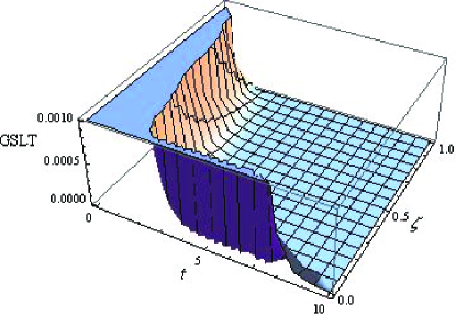
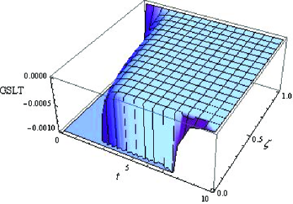
Figure 1: Validity of GSLT for the model (27). The left plot is for $c_{1}=c_{2}=1$ and right for $c_{1}=1$ with $c_{2}=-1$.

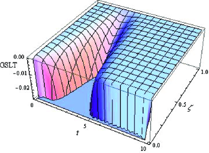
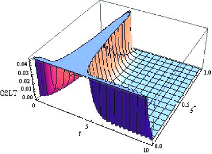
Figure 2: Validity of GSLT for the model (27). The left plot is for $c_{1}=-1$ with $c_{2}=1$ and right for $c_{1}=c_{2}=-1$.

Figures 1 and 2 show the validity of GSLT for the model (27) in the background of flat FRW universe model. The present day value of Hubble parameter is $H_{0}=(67.8\pm 0.9)~{}\mathrm{kms}^{-1}\mathrm{Mpc}^{-1}$ at the $68\%$C.L. (C.L. stands for confidence level) which can be considered as $0.67$ in units of $100~{}\mathrm{kms}^{-1}\mathrm{Mpc}^{-1}$ [25, 26]. The value of matter density parameter is constrained as $0.308\pm 0.012$ with $68\%$C.L. whereas scale factor at $t_{0}=13.7~{}\mathrm{Gyr}$ is $a_{0}=1$ [25]. For this model, we have four parameters $c_{1},~{}c_{2},~{}\zeta$ and $t$ with fixed values of $H_{0}=0.67,~{}a_{0}=1$ and $\rho_{0}=0.3$. Here, we examine the validity of GSLT against two parameters $\zeta$ and $t$ with four possible choices of integration constants. For the case $(c_{1},c_{2})>0$, we find that the validity of GSLT holds for the considered intervals of $\zeta$ and $t$. Figure 1 (left) indicates the validity for $c_{1}=c_{2}=1$ while the right plot corresponds to the case $c_{1}>0$ and $c_{2}<0$. The left plot of Figure 2 shows that the validity of GSLT is not true for $c_{1}<0$ with $c_{2}>0$ while it satisfies for both negative values of $(c_{1},c_{2})$ as shown in the right panel. It is found that the generalized second law holds at all times only for the same signatures of integration constants.

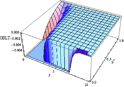
Figure 3: Validity of GSLT for the model (LABEL:5c). The left plot is for $c_{1}=c_{2}=1$ and right for $c_{1}=1$ with $c_{2}=-1$.

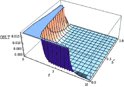
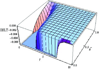
Figure 4: Validity of GSLT for the model (LABEL:5c). The left plot is for $c_{1}=-1$ with $c_{2}=1$ and right for $c_{1}=c_{2}=-1$.

The graphical behavior of GSLT for de Sitter $f(\mathcal{G},T)$ model (LABEL:5c) is shown in Figures 3 and 4 against parameters $\zeta$ and $t$. In this case, we have considered $H_{0}=0.67,~{}a_{0}=1$ and $\rho_{0}=0.3$ with four possible signature choices of integration constants $c_{1}$ and $c_{2}$ as in the previous model. Figure 3 (right) and Figure 4 (left) show that GSLT is true for all considered values of $\zeta$ and $t$ with opposite signatures of $(c_{1},c_{2})$. For model (LABEL:5c), the choice of same signatures of integration constants is ruled out since it does not provide feasible region for which GSLT holds.

4.2 Power-law Solution

Power-law solution has remarkable importance in modified theories of gravity to discuss the decelerated as well as accelerated cosmic evolutionary phases which are characterized by the scale factor as [27]

$$a(t)=a_{0}t^{\beta},\quad H=\frac{\beta}{t},\quad\beta>0.$$ (29)

The accelerated phase of the universe is observed for $\beta>1$ while $0<\beta<1$ covers the decelerated phase including dust $(\beta=\frac{2}{3})$ as well as radiation $(\beta=\frac{1}{2})$ dominated cosmic epochs. For this scale factor, the energy density and GB invariant becomes

$$\rho=\rho_{0}t^{-3\beta},\quad\mathcal{G}=24\frac{\beta^{3}}{t^{4}}(\beta-1).$$ (30)

Using Eqs.(29) and (30) in (25), the validity condition for GSLT takes the form

$$\frac{1+a_{0}^{4}\beta^{3}(\beta-1)t^{-4}(a_{0}^{2}\beta^{2}t^{-2}+kt^{-2\beta})^{-2}}{\zeta(8\pi G+f_{T})}\left[\frac{\beta}{t}(2-\zeta)\left(\frac{\beta a_{0}^{2}t^{-2}+kt^{-2\beta}}{\beta^{2}a_{0}^{2}t^{-2}+kt^{-2\beta}}\right)^{2}\right.$$

$$- \left.2\frac{\beta}{t}(1-\zeta)\left(\frac{\beta a_{0}^{2}t^{-2}+kt^{-2\beta}}{\beta^{2}a_{0}^{2}t^{-2}+kt^{-2\beta}}\right)-\frac{\zeta-1}{8\pi G+f_{T}}\left(96\frac{\beta^{3}}{t^{5}}(\beta-1)f_{\mathcal{G}T}\right.\right.$$

$$+ \left.\left.3\beta\rho_{0}t^{-4}f_{TT}\right)\right]\geq 0.$$

The reconstructed $f(\mathcal{G},T)$ model for dust fluid is given by [5]

$$f(\mathcal{G},T)=d_{1}d_{3}T^{d_{2}}\mathcal{G}^{\frac{1}{4}(\alpha_{1}+\alpha_{2})}+d_{2}d_{3}T^{d_{2}}\mathcal{G}^{\frac{1}{4}(\alpha_{1}-\alpha_{2})}+d_{1}d_{2}T^{\alpha_{3}}+\alpha_{4}T+\alpha_{5}T^{\alpha_{6}},$$

where $d_{l}$’s $(l=1,2,3)$ are integration constants and

$$\alpha_{1} = \frac{1}{2}\left[5-\beta(1+3d_{2})\right],$$

$$\alpha_{2} = \left[\frac{3}{4}\beta d_{2}\{3d_{2}\beta+2(\beta-1)-8\}+\frac{1}{4}(\beta-1)(\beta+7)+4+8d_{2}(\beta-1)\right]^{\frac{1}{2}},$$

$$\alpha_{3} = -\frac{1}{2},\quad\alpha_{4}=-\frac{16\pi G}{3},\quad\alpha_{5}=\left(\frac{18\beta^{3}}{3\beta+4}\right)\rho_{0}^{-\frac{2}{3\beta}},\quad\alpha_{6}=\frac{2}{3\beta},$$

imply that the conservation law holds. The continuity constraint splits this model into two functions with some additional constants as

$$f_{1}(\mathcal{G},T) = d_{1}d_{3}\gamma_{1}T^{d_{2}}\mathcal{G}^{\frac{1}{4}(\alpha_{1}+\alpha_{2})}+d_{1}d_{2}\gamma_{2}T^{\alpha_{3}}+\gamma_{3}T+\gamma_{4}T^{\alpha_{6}},$$ (31)

$$f_{2}(\mathcal{G},T) = d_{2}d_{3}\gamma_{5}T^{d_{2}}\mathcal{G}^{\frac{1}{4}(\alpha_{1}-\alpha_{2})}+d_{1}d_{2}\gamma_{6}T^{\alpha_{3}}+\gamma_{7}T+\gamma_{8}T^{\alpha_{6}},$$ (32)

where

$$\gamma_{1} = 1-\frac{\alpha_{7}}{\alpha_{8}},\quad\gamma_{2}=1-\frac{\alpha_{3}^{2}}{\alpha_{8}},\quad\gamma_{3}=\alpha_{4}\left(1-\frac{1}{\alpha_{8}}\right),\quad\gamma_{4}=\alpha_{5}\left(1-\frac{\alpha_{6}^{2}}{\alpha_{8}}\right),$$

$$\gamma_{5} = 1-\frac{\alpha_{8}}{\alpha_{7}},\quad\gamma_{6}=1-\frac{\alpha_{3}^{2}}{\alpha_{7}},\quad\gamma_{7}=\gamma_{4}\left(1-\frac{1}{\alpha_{7}}\right),\quad\gamma_{8}=\gamma_{5}\left(1-\frac{\alpha_{6}^{2}}{\alpha_{7}}\right),$$

$$\alpha_{7} = \frac{d_{2}}{6\beta}\left[6d_{2}\beta-3\beta+2(\alpha_{1}+\alpha_{2})\right],\quad\alpha_{8}=\frac{d_{2}}{6\beta}\left[6d_{2}\beta-3\beta+2(\alpha_{1}-\alpha_{2})\right].$$

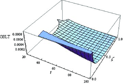
Figure 5: Validity of GSLT for the model (31). The left plot is for $d_{1}=d_{3}=1$ and right for $d_{1}=1$ and $d_{3}=-1$.

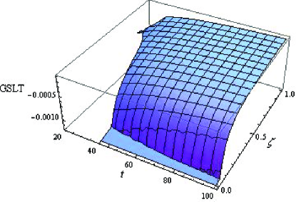
Figure 6: Validity of GSLT for the model (31). The left plot is for $d_{1}=-1$ with $d_{3}=1$ and right for $d_{1}=d_{3}=-1$.

The validity of GSLT for models (31) and (32) depend on five parameters $d_{1},~{}d_{2},~{}d_{3},~{}\zeta$ and $t$. Figure 5 and 6 show the behavior of GSLT for power-law reconstructed $f(\mathcal{G},T)$ model (31). We examine the validity against $\zeta$ and $t$ with $a_{0}=1,~{}\rho_{0}=0.3,~{}n=\frac{2}{3}$ and $d_{2}=-1.64285$ while the behavior of remaining two integration constants $d_{2}$ and $d_{3}$ are investigated for four possible choices of their signatures. Figure 5 shows that GSLT is satisfied for both cases $d_{3}>0$ and $d_{3}<0$ with $d_{1}>0$ in the considered interval of parameters $(\zeta,t)$. We also check that the validity region decreases as the value of integration constants increase positively as well as negatively. Figure 6 shows that GSLT does not hold for model (31) when $d_{3}>0$ and $d_{3}<0$ with $d_{1}<0$. From both figures, it is found that the signature of $d_{1}$ has dominant effect on the validity of GSLT as compared to $d_{3}$.

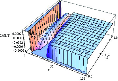
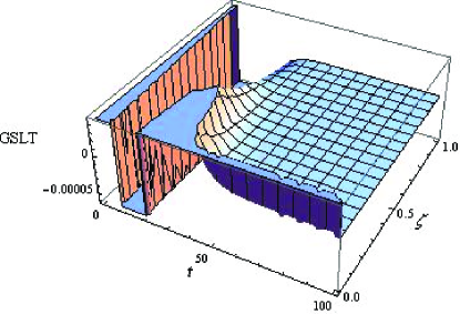
Figure 7: Validity of GSLT for the model (32). The left plot is for $d_{1}=d_{3}=1$ and right for $d_{1}=1$ and $d_{3}=-1$.

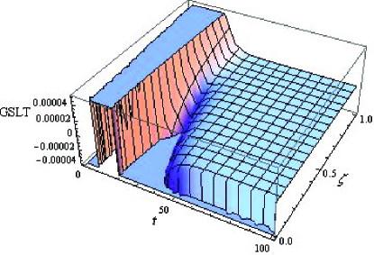
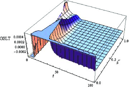
Figure 8: Validity of GSLT for the model (32). The left plot is for $d_{1}=-1$ with $d_{3}=1$ and right for $d_{1}=d_{3}=-1$.

The validity of GSLT for the model (32) is shown in Figures 7 and 8. For this model, the viability of law again depends on five parameters $d_{1},~{}d_{2},~{}d_{3},~{}\zeta$ and $t$ while we set $a_{0}=1,~{}\rho_{0}=0.3,~{}n=\frac{2}{3}$ and $d_{2}=7.5$. The left panel shows that this law is satisfied for all values of $\zeta$ at the initial times as well as when $\zeta$ approaches to $1$ with $t\geq 27$ for the case $(d_{1},d_{3})>0$ while the feasible region for $d_{1}>0$ and $d_{3}<0$ is shown in the right plot. Similarly, Figure 8 shows the regions where GSLT holds for the remaining two signatures of $(d_{1},d_{3})$. In this case, we observe that validity of GSLT is true for all four possible choices of integration constants for the specific ranges of $\zeta$ and $t$.

5 Concluding Remarks

In this paper, we have investigated the first and second laws in the non-equilibrium description of thermodynamics and also checked the validity of GSLT for reconstructed models in $f(\mathcal{G},T)$ gravity. The thermodynamical laws are studied at the apparent horizon of FRW universe model with any spatial curvature parameter $k$. We have found that the total entropy in the first law of thermodynamics involves contribution from horizon entropy in terms of area and the entropy production term. This second term appears due to non-equilibrium behavior which implies that some energy is exchanged between outside and inside the apparent horizon. It is worth mentioning here that no such auxiliary entropy production term appears in GR, GB, Lovelock and braneworld theories of gravity [12, 13].

We have found the general expression for the validity of GSLT in terms of horizon entropy, entropy production term as well as entropy corresponding to all matter and energy contents inside the horizon. For non-equilibrium picture of thermodynamics, it is assumed that temperature associated with all matter and energy contents inside the horizon is always positive and smaller than the temperature at apparent horizon. It is found that viability condition for this law is consistent with the universal condition for its validity in modified theories of gravity [14]. We have also investigated the validity condition of GSLT for the equilibrium description of thermodynamics. The validity of this law for the reconstructed $f(\mathcal{G},T)$ models (de Sitter universe and power-law solution) for the dust fluid [5, 8] is also studied. The results can be summarized as follows.

• For de Sitter reconstructed models, it is found that the validity of GSLT is true for model (27) when the integration constants $(c_{1},c_{2})$ have same signatures while for the second model (LABEL:5c), the feasible regions are obtained for the opposite signatures (Figures 1-4).

• For power-law reconstructed models, the valid results are found when integration constant $d_{1}$ is positive for the model (31) while for the model (32), this holds for all possible choices of $d_{1}$ and $d_{3}$ (Figures 5-8).

We conclude that the validity condition of GSLT is true for both reconstructed de Sitter and power-law $f(\mathcal{G},T)$ models with suitable choices of free parameters.

Acknowledgment

We would like to thank the Higher Education Commission, Islamabad, Pakistan for its financial support through the Indigenous Ph.D. 5000 Fellowship Program Phase-II, Batch-III.

The authors have no conflict of interest.

References

• [1] Bhawal, B. and Kar, S.: Phys. Rev. D 46(1992)2464; Deruelle, N. and Dole$\check{z}$el, T.: Phys. Rev. D 62(2000)103502; De Felice, A. and Tsujikawa, S.: Living Rev. Rel. 13(2010)3.
• [2] Nojiri, S. and Odintsov, S.D.: Phys. Lett. B 631(2005)1.
• [3] Cognola, G. et al.: Phys. Rev. D 73(2006)084007; De Felice, A. and Tsujikawa, S.: Phys. Lett. B 675(2009)1; Phys. Rev. D 80(2009)063516.
• [4] Harko, T. et al.: Phys. Rev. D 84(2011)024020.
• [5] Sharif, M. and Ikram, A.: Eur. Phys. J. C 76(2016)640.
• [6] Sharif, M. and Ikram, A.: Int. J. Mod. Phys. D 26(2017)1750084.
• [7] Shamir, M.F. and Ahmad, M.: Eur. Phys. J. C 77(2017)55.
• [8] Sharif, M. and Ikram, A.: Phys. Dark Universe 17(2017)1.
• [9] Bardeen, J.M., Carter, B. and Hawking, S.W.: Commun. Math. Phys. 31(1973)161; Bekenstein, J.D.: Phys. Rev. D 7(1973)2333; Hawking, S.W.: Commun. Math. Phys. 43(1975)199; ibid. 46(1976)206.
• [10] Jacobson, T.: Phys. Rev. Lett. 75(1995)1260.
• [11] Cai, R.G. and Kim, S.P.: J. High Energy Phys. 02(2005)050.
• [12] Akbar, M. and Cai, R.G.: Phys. Rev. D 75(2007)084003.
• [13] Eling, C., Guedens, R. and Jacobson, T.: Phys. Rev. Lett. 96(2006)121301; Cai, R.G. and Cao, L.M.: Phys. Rev. D 75(2007)064008; Akbar, M. and Cai, R.G.: Phys. Lett. B 648(2007)243; Sheykhi, A., Wang, B. and Cai, R.G.: Nucl. Phys. B 779(2007)1; Cai, R.G. et al.: Phys. Rev. D 78(2008)124012.
• [14] Wu, S.F. et al.: Class. Quantum Grav. 25(2008)235018.
• [15] Bamba, K. and Geng, C.Q.: Phys. Lett. B 679(2009)282.
• [16] Sadjadi, H.M.: Europhys. Lett. 92(2010)50014.
• [17] Bamba, K. and Geng, C.Q.: J. Cosmol. Astropart. Phys. 11(2011)008.
• [18] Sharif, M. and Zubair, M.: J. Cosmol. Astropart. Phys. 03(2012)028.
• [19] Abdolmaleki, A. and Najafi, T.: Int. J. Mod. Phys. D 25(2016)1650040.
• [20] Landau, L.D. and Lifshitz, E.M.: The Classical Theory of Fields (Pergamon Press, 1971).
• [21] Wald, R.M.: Phys. Rev. D 48(1993)R3427.
• [22] Jacobson, T. and Kang, G.: Phys. Rev. D 49(1994)6587; Iyer, V. and Wald, R.W.: Phys. Rev. D 50(1994)846; Maeda H.: Phys. Rev. D 81(2010)124007.
• [23] Brustein, R., Gorbonos, D. and Hadad, M.: Phys. Rev. D 79(2009)0444025.
• [24] Sadjadi, H.M.: Phys. Scr. 83(2011)055006; Sharif, M. and Fatima, I.: Astrophys. Space Sci. 354(2014)507.
• [25] Ade, P.A.R. et al.: Astron. Astrophys. 594(2016)A13.
• [26] Sereno, M. and Paraficz, D.: Mon. Not. R. Astron. Soc. 437(2014)600.
• [27] de la Cruz-Dombriz, ร. and Sรกez-Gรณmez, D.: Class. Quantum Grav. 29(2012)245014.