Intrinsic charm contribution to the prompt atmospheric neutrino flux

Abstract

In this work we investigate the impact of intrinsic charm on the prompt atmospheric neutrino flux. The color dipole approach to heavy quark production is generalized to include the contribution of processes initiated by charm quarks. The prompt neutrino flux is calculated assuming the presence of intrinsic charm in the wave function of the projetile hadron. The predictions are compared with previous color dipole results which were obtained taking into account only the process initiated by gluons. In addition, we estimate the atmospheric (conventional + prompt) neutrino flux and compare our predictions with the ICECUBE results for the astrophysical neutrino flux. Our results demonstrate that the contribution of the charm quark initiated process is non - negligible and that the prompt neutrino flux can be enhanced by a factor $\approx$ 2 at large neutrino energies if an intrinsic charm component is present in the proton wave function.

I Introduction

Astrophysical neutrinos detected by the IceCube Observatory mark the beginning of neutrino astronomy IceCube_Science ; Aartsen:2014gkd ; Aartsen:2016xlq , which allows us to study very high energy physical processes in the Universe review_icecube ; annual_mezsaros . The atmospheric neutrino flux is produced in the atmosphere of the Earth (through cosmic-ray interactions with nuclei) and it is the main background in studies of cosmic neutrinos. During the last years, several neutrino observatories Abbasi:2010ie ; Aartsen:2012uu ; Adamson:2012gt ; Fukuda:1998ub have studied the high-energy neutrino flux. The experimental data indicate that, at low energies ($E_{\nu}\lesssim 10^{5}$ GeV), the measured neutrino flux is dominated by atmospheric neutrinos which come from the decay of light mesons (pions and kaons). This flux is called conventional atmospheric neutrino flux Honda:2006qj ; Barr:2004br ; Gaisser:2014pda . On the other hand, in the energy range 10⁵ GeV $<E_{\nu}<$ 10⁷ GeV, the prompt atmospheric neutrino flux (resulting from the decay of heavy quark hadrons) becomes important ingelman ; Martin:2003us ; sigl . The precise knowledge of this contribution is crucial for the determination of the cosmic neutrino flux.

The calculation of the prompt atmospheric neutrino flux has been subject of intense activity enb_stasto1 ; sigl ; rojo1 ; enb_stasto2 ; rojo2 ; halzen ; laha ; prosa ; sigl2 . Since heavy quarks are an important source of neutrinos, it became necessary to describe their production with better accuracy. Different treatments (and approximations) of heavy quark production at high energies and of the QCD dynamics at small values of the Bjorken - $x$ variable were proposed. Although the LHC data on the prompt heavy quark cross sections (see e.g. Refs. Aaij:2013mga ; Aaij:2015bpa ) helped us to improve the description of heavy meson production at forward rapidities and significantly reduced some of the theoretical uncertainties, the predictions obtained by different groups can still differ by a factor $\geq 2$. This large uncertainty is due to the fact that the main contribution to the prompt neutrino flux comes from heavy quark production in a kinematical range which is not currently probed by the LHC. In Ref. vicantoni the authors have presented a detailed analysis of the kinematical domains in which charm and prompt atmospheric neutrino production from cosmic rays are relevant for the IceCube experiment. They explored the sensitivity of the corresponding neutrino flux and of the charm cross section to the cuts on the maximal $pp$ c.m. energy, to the longitudinal momentum fraction in the target and projectile, to the Feynman $x_{F}$ and to $p_{T}$ values included in the calculation. They have demonstrated that in order to address the production of high-energy neutrinos ($E_{\nu}>$ 10⁷ GeV) one needs to know the charm production cross section at energies larger than those available at the LHC as well as the parton/gluon distributions in the region 10^-8 $<x<$ 10^-5, which are not presently available in collider measurements. Consequently, the presence of new effects, which are expected to contribute to small values of $x$ and/or large values of the $x_{F}$, cannot be excluded by current data.

The production of heavy states at high energies is expected to be sensitive to non - linear effects of QCD dynamics kt_hq ; hq_sat ; vicmag ; cgn ; wata ; armesto , which are predicted to be enhanced at forward rapidites cgc . The cross sections at forward rapidities are dominated by collisions of projectile partons with large light cone momentum fractions ($x_{p}\rightarrow 1$) with target partons carrying a very small momentum fraction ($x_{t}\ll 1$). Consequently, small-$x$ effects coming from the non-linear aspects of QCD and from the physics of the Color Glass Condensate (CGC) cgc are expected to appear and the usual factorization formalism is expected to break down hq_sat . Recent results dhj ; buw ; ptmedio.nois indicate that the CGC formalism provides a satisfactory description of the experimental data on particle production at forward rapidities. Additionally, large - $x$ effects in the projectile are also expected to contribute to heavy quark production at forward rapidities. One of the possible new effects is the presence of intrinsic heavy quarks in the hadron wave function (For recent reviews see, e.g. Refs. review_brod_adv ; review_brod_prog ). Heavy quarks in the sea of the proton can be perturbatively generated by gluon splitting. Quarks generated in this way are usually denoted extrinsic heavy quarks. In contrast, the intrinsic heavy quarks have multiple connections to the valence quarks of the proton and thus are sensitive to its nonperturbative structure.

The existence of the intrinsic charm (IC) component was first proposed long ago in Ref. bhps (see also Ref. hal ) and since then other models of IC have been discussed pnndb ; wally99 . Its existence implies a large enhancement of the charm distribution at large $x$ ($>0.1$) in comparison to the extrinsic charm prediction. Moreover, due to the momentum sum rule, the gluon distribution is also modified by the inclusion of intrinsic charm. The intrinsic charm (IC) component of the proton wave function was included in recent global analyses, performed by different theoretical groups, in order to constrain the parton distributions. Although the resulting IC distributions are compatible with the world data, the amount of IC in the proton wave function is still subject of intense debate wally16 ; brod_letter and has motivated a large number of phenomenological studies (See e.g. Refs. russos ; bailas ; biw16 ).

One of the most direct consequences of the intrinsic charm component is that it gives rise to heavy mesons with large fractional momenta relative to the beam particles, affecting the $x_{F}$ and rapidity distribution of charmed particles. This aspect was explored e.g. in Refs. ingelman ; kniehl ; npanos ; prdnos . In particular, in Ref. prdnos we studied $D$ - meson production at forward rapidities taking into account non - linear effects in the QCD dynamics and the intrinsic charm (IC) component of the proton wave function. The results show that, at the LHC, the intrinsic charm component changes the $D$ rapidity distributions in a region which is beyond the coverage of the LHCb detector. At higher energies, as those probed in neutrino observatories, our results indicated that the IC component dominates the rapidity and $x_{F}$ distributions, with the latter being enhanced by a factor 6 – 8 in the $0.2\leq x_{F}\leq 0.8$ range. In Ref. prdnos we have pointed out that one of the basic consequences of this enhancement is the modification of the prompt neutrino flux at large energies. The main purpose of this work is to estimate the impact of the intrinsic charm component on the prompt neutrino flux taking into account non - linear effects in the QCD dynamics. It is important to emphasize that the contribution associated to a heavy quark in the initial state was not taken into account in previous studies using the color dipole formalism performed e.g. in Refs. ers ; enb_stasto2 . The inclusion of heavy quarks in the initial state in the color dipole approach is done here for the first time. Additionally, previous estimates of the intrinsic charm contribution to the neutrino flux laha ; halzen have made use of phenomenological models of the $x_{F}$ - distribution in $\Lambda_{c}$ and $D$ production, constrained only by the scarce low energy experimental data and then extrapolated to higher energies. In contrast, in our analysis the basic ingredients of the calculations, the charm/gluons PDF’s and the dipole - hadron amplitude, have been constrained by the most recent LHC data and non - linear effects in the QCD dynamics are taken into account.

This paper is organized as follows. In the next Section we present a brief review of the formalism to calculate the charm production at forward rapidities, as well as we discuss the impact of an intrinsic charm component in the Feynman $x_{F}$ - distribution. In Section III we present our results for the prompt neutrino flux. The contribution of the different components is analyzed and the impact of the intrinsic component is estimated. In particular, the predictions for the atmospheric (conventional + prompt) neutrino flux is compared with the recent ICECUBE results for the flux of the astrophysical neutrinos. Finally, in Section IV we summarize our main results and conclusions.

II Formalism

In the analysis performed in this paper, we will closely follow the procedure described in detail in Refs. vicantoni ; prdnos . In what follows we will only present the main aspects of the formalism and refer the reader to Refs. vicantoni ; prdnos for more details. As in Ref. vicantoni , we will calculate the prompt neutrino flux using the semi-analytical $Z$-moment approach, proposed many years ago in Ref. ingelman and discussed in detail e.g. in Refs. ers ; rojo1 . In this approach, a set of coupled cascade equations for the nucleons, heavy mesons and leptons (and their antiparticles) fluxes is solved, with the equations being expressed in terms of the nucleon-to-hadron ($Z_{NH}$), nucleon-to-nucleon ($Z_{NN}$), hadron-to-hadron ($Z_{HH}$) and hadron-to-neutrino ($Z_{H\nu}$) $Z$-moments. These moments are inputs in the calculation of the prompt neutrino flux associated with the production of a heavy hadron $H$ and its decay into a neutrino $\nu$ in the low- and high-energy regimes. We will focus on vertical fluxes and will assume that the cosmic ray flux $\phi_{N}$ can be described by a broken power-law spectrum prs or by the H3a spectrum proposed in Ref. gaisser , with the incident flux being represented by protons. Moreover, we will assume that the charmed hadron $Z$-moments can be expressed in terms of the charm $Z$-moment as follows: $Z_{pH}=f_{H}\times Z_{pc}$, where $f_{H}$ is the fraction of charmed particle which emerges as a hadron $H$. As in Ref. ers , we will assume that $f_{D^{0}}=0.565$, $f_{D^{+}}=0.246$, $f_{D_{s}^{+}}=0.080$ and $f_{\Lambda_{c}}=0.094$.

The charm $Z$-moment at high energies can be expressed by

$$Z_{pc}(E)=\int_{0}^{1}\frac{dx_{F}}{x_{F}}\frac{\phi_{p}(E/x_{F})}{\phi_{p}(E)}\frac{1}{\sigma_{pA}(E)}\frac{d\sigma_{pA\rightarrow charm}(E/x_{F})}{dx_{F}}\,\,,$$ (1)

where $E$ is the energy of the produced particle (charm), $x_{F}$ is the Feynman variable, $\sigma_{pA}$ is the inelastic proton-Air cross section, which we assume to be given as in Ref. sigl , and $d\sigma/dx_{F}$ is the differential cross section for the charm production, which we assume to be given by $d\sigma_{pA\rightarrow charm}/dx_{F}=2\,d\sigma_{pA\rightarrow c\bar{c}}/dx_{F}$. One of the main inputs in the $Z$-moment approach is the Feynman $x_{F}$ distribution of the heavy quarks produced in hadronic collisions. As discussed in Ref. vicantoni , the main contribution to the prompt neutrino flux comes from large values of $x_{F}$, that are associated with heavy quark production at forward rapidities. Moreover, as the production of neutrinos at a given neutrino energy, $E_{\nu}$, is determined by collisions of cosmic rays with nuclei in the atmosphere at energies that are a factor of order 100-1000 larger, the prompt neutrino flux measured in the kinematical range that is probed by the IceCube Observatory and future neutrino telescopes is directly associated with the treatment of the heavy quark production cross section at high energies. Following Ref. prdnos , we will use the approaches developed in Refs. nnz ; boris and npanos for the treatment of heavy quark production induced by gluon - gluon and charm - gluon interactions, respectively, and we will take into account non - linear effects in the QCD dynamics. The contribution of the $q\bar{q}\rightarrow c\bar{c}$ subprocess will be disregarded, since it is negligible at the energies and rapidities relevant for the prompt neutrino flux vicantoni .

The basic idea in Ref. prdnos is that at forward rapidities, the projectile (dilute system) evolves according to the linear DGLAP dynamics and the target (dense system) is treated using the CGC formalism. In this approach, the charm $x_{F}$ - distribution will be determined by the contribution of the two diagrams presented in Fig. 1, which are associated to the gluon and charm - initiated processes. The first contribution, represented in Fig. 1 (a), can be estimated using the color dipole picture nnz ; boris , which implies that the rapidity distribution for the charm production in a $h_{1}h_{2}$ collision can be expressed as follows

$$\frac{d\sigma}{dy}=x_{1}g^{h_{1}}(x_{1},\mu_{F}^{2})\,\sigma(gh_{2}\rightarrow\{c\bar{c}\}X)\,\,,$$ (2)

where $x_{1}g_{p}(x_{1},\mu_{F})$ is the projectile gluon distribution, the cross section $\sigma(gh_{2}\rightarrow\{c\bar{c}\}X)$ describes charm production in a gluon - nucleon interaction, $y$ is the rapidity of the pair and $\mu_{F}$ is the factorization scale. Moreover, the cross section of the process $g+h_{2}\rightarrow c\bar{c}X$ is given by:

$$\sigma(gh_{2}\rightarrow\{c\bar{c}\}X)=\int_{0}^{1}d\alpha\int d^{2}\mbox{\boldmath$r$}\,\,|\Psi_{g\rightarrow c\bar{c}}(\alpha,\mbox{\boldmath$r$})|^{2}\,\,\sigma^{h_{2}}_{c\bar{c}g}(\alpha,\mbox{\boldmath$r$})$$ (3)

where $\alpha$ ($\bar{\alpha}\equiv 1-\alpha$) is the longitudinal momentum fraction carried by the quark (antiquark), $r$ is the transverse separation of the pair, $\Psi_{g\rightarrow c\bar{c}}$ is the light-cone (LC) wave function of the transition $g\rightarrow c\bar{c}$ (which is calculable perturbatively and is proportional to $\alpha_{s}$) and $\sigma^{h_{2}}_{c\bar{c}g}$ is the scattering cross section of a color neutral quark-antiquark-gluon system on the hadron target $h_{2}$ nnz ; boris . The three - body cross section is given in terms of the dipole - nucleon cross section $\sigma_{c\bar{c}}$ as follows:

$$\sigma^{h_{2}}_{c\bar{c}g}(\alpha,\mbox{\boldmath$r$})=\frac{9}{8}[\sigma_{c\bar{c}}(\alpha\mbox{\boldmath$r$})+\sigma_{c\bar{c}}(\bar{\alpha}\mbox{\boldmath$r$})]-\frac{1}{8}\sigma_{c\bar{c}}(\mbox{\boldmath$r$})\,\,.$$ (4)

Finally, the dipole - nucleon cross section can be expressed in terms of the forward scattering amplitude ${\cal{N}}(x,\mbox{\boldmath$r$})$, which is determined by the QCD dynamics, as follows:

$$\sigma_{c\bar{c}}(x,\mbox{\boldmath$r$})=\sigma_{0}{\cal N}(x,\mbox{\boldmath$r$})$$ (5)

where $\sigma_{0}$ is a free parameter usually determined by a fit of the HERA data. On the other hand, the contribution of the charm initiated process, represented in Fig. 1 (b), is given by npanos

$${d\sigma\over dy}={1\over(2\pi)^{2}}\int d^{2}p_{T}f_{c/h_{1}}(x_{1},\mu_{F}^{2})\,\,\sigma_{0}\,\widetilde{\cal N}\left(x_{2},{p_{T}}\right)\,.$$ (6)

where $x_{1,2}$ is defined by $x_{1,2}=p_{T}e^{\pm y}/\sqrt{s}$, $f_{c/h_{1}}$ represents the projectile charm distribution and $\widetilde{\cal N}(x,{p_{T}})$ is the Fourier transform of the scattering amplitude ${\cal N}(x,\mbox{\boldmath$r$})$.

In order to estimate the contributions of the gluon and charm - initiated processes, described by Eqs. (2) and (6), we should to assume a model to describe the dipole - nucleon scattering amplitude ${\cal N}(x_{2},\mbox{\boldmath$r$})$, as well as a parametrization for gluon and charm distributions in the projectile. The the dipole - nucleon scattering amplitude ${\cal N}(x_{2},\mbox{\boldmath$r$})$ describes the interaction of a color dipole of size $r$ with the nucleon and involves the QCD dynamics at high energies. Such quantity contains all the information about the initial state of the hadronic wavefunction and therefore about the non-linearities and quantum effects which are characteristic of a system such as the CGC (For reviews, see e.g. cgc ). Formally its evolution is usually described in the mean field approximation of the CGC formalism by the BK equation bk . Its analytical solution is known only in some special cases. Advances have been made in solving the BK equation numerically la11 . Since the BK equation still lacks a formal solution in all kinematical space, several groups have constructed phenomenological models for the dipole scattering amplitude. These models have been used to fit the RHIC, LHC and HERA data dhj ; buw ; dips ; IIM ; Soyez . As in Ref. prdnos , in our analysis we will use the BUW model for ${\cal N}$, originally proposed in Ref. buw , which assumes that ${\cal{N}}$ can be modelled through a simple Glauber-like formula,

$${\cal{N}}(x,\mbox{\boldmath$r$})=1-\exp\left[-\frac{1}{4}(\mbox{\boldmath$r$}^{2}Q_{s}^{2}(x))^{\gamma(x,\mbox{\boldmath$r$}^{2})}\right]\,\,,$$ (7)

where $Q_{s}(x)$ is the saturation scale and $\gamma$ is the anomalous dimension of the target gluon distribution. The speed with which we move from the non-linear regime to the extended geometric scaling regime and then from the latter to the linear regime is what differs the BUW from other phenomenological models. This transition speed is dictated by the behavior of the anomalous dimension $\gamma(x,\mbox{\boldmath$r$}^{2})$, which is assumed in the BUW buw dipole model to be given by

$$\gamma(\omega=p_{T}/Q_{s})_{BUW}=\gamma_{s}+(1-\gamma_{s})\frac{(\omega^{a}-1)}{(\omega^{a}-1)+b}$$ (8)

where $a$, $b$ and $\gamma_{s}$ are free parameters to be fixed by fitting experimental data. In Ref. ptmedio.nois , the original parameters of the BUW model were updated in order to make this model compatible with all existing data. In particular, the recent LHC data on light hadron production at forward rapidity are satisfactorily reproduced by the updated model.

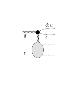
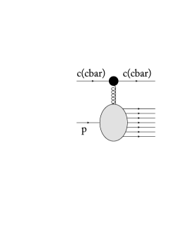
(a)		(b)

Figure 1: Contributions to charm production at high energies and forward rapidities. (a) Contribution from gluon - initiated processes. (b) Contribution from charm in the initial state.

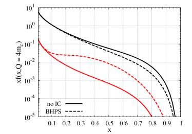
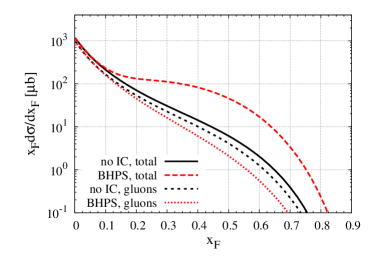
(a)		(b)

Figure 2: (a) Comparison between the BHPS and No IC predictions for the charm (lower red curves) and gluon (upper black curves) distributions. (b) Comparison between the BHPS and No IC predictions for the Feynman $x_{F}$ distributions considering $pp$ collisions at $\sqrt{s}=13$ TeV.

In order to quantify the impact of the intrinsic charm component on the projectile wave function, we will use in our calculations the next - to - leading order CTEQ 6.5 parametrization for the parton distributions cteq . In Ref. cteq , the CTEQ group determined the shape and normalization of the IC distribution in the same way as they do for other parton species. In fact, they find several IC distributions which were compatible with the world data. In what follows we will only consider the parametrization based on the BHPS model bhps , obtained assuming that the average longitudinal momentum fraction carried by the charm and anticharm is $\langle x_{c\bar{c}}\rangle=2\%$ at the initial scale of the QCD evolution. The BHPS model assumes that the nucleon light cone wave function has higher Fock states, one of them being $|qqqc\overline{c}>$. The probability of finding the nucleon in this configuration is given by the inverse of the squared invariant mass of the system. Because of the heavy charm mass, this probability as a function of the quark fractional momentum, $P(x)$, is very hard, as compared to the one obtained through the DGLAP evolution. Such assumptions are used to describe the shape of the parametrization at the initial scale of the DGLAP evolution, which is evolved for larger scales in order to contrain, by a global data fit procedure, the parton distributions of the proton. In Fig. 2 (a) we compare the predictions of the BHPS model with those obtained disregarding the presence of an intrinsic component (denoted No-IC hereafter). In the case of the charm distribution (lower red curves), the BHPS model predict a large enhancement of the distribution at large $x$ ($>0.1$). In Fig. 2 (a) we also present the corresponding gluon distributions (upper black curves). Due to the momentum sum rule, the gluon distribution is also modified by the inclusion of intrinsic charm. In particular, the BHPS model imply a suppression in the gluon distribution at large $x$. The impact of these different models on the Feynman $x_{F}$ distribution for the charm production in $pp$ collisions at $\sqrt{s}=13$ TeV is presented in Fig. 2 (b). We present the sum of the gluon and charm contributions, denoted “total” in the figure, as well present separately the gluon contribution. We have that in the No IC case, the distribution is dominated by the gluon initiated process. In contrast, when intrinsic charm is included, the behavior of the distribution in the intermediate $x_{F}$ range ($0.2\leq x_{F}\leq 0.8$) is strongly modified. It is important to emphasize that the contribution of the gluonic component decreases in this kinematical range, as expected from the analysis of the parton distributions presented in Fig. 2 (a). As we will show in the next Section, these modifications in the distribution, associated the presence of an intrinsic component, has important implications in the prompt neutrino flux.

Before to present our predictions for the prompt neutrino flux in the next Section, two comments are in order. In our analysis we will consider the next - to - leading order CTEQ 6.5C parametrization for the parton distributions cteq , which is provided by the CTEQ group. It is important to emphasize that the CTEQ-TEA group has also performed a global analysis of the recent experimental data including an intrinsic charm component, which is available in the CT14 parametrization cteq14 . However, this analysis has been performed at next-to-next-to-leading order. As demonstrated in Ref. rauf , the predictions of the dipole approach for the charm production agree with those obtained using the collinear formalism at NLO, in the kinematical range where the equivalence between the approaches is expected. Therefore, we believe that it is more consistent to use in our calculations PDFs obtained at NLO. Second, the CTEQ 6.5C parametrization is used in this paper for consistence with our previous study prdnos , where we have performed a detailed analysis of the $D$ - meson production at the LHC energies considering different models for the intrinsic charm component. In particular, in Ref. prdnos we have compared the BHPS predictions with those obtained using the Meson Cloud model pnndb ; wally99 . Such model is not considered in the CTEQ 6.6C parametrization, which is an improved version of CTEQ 6.5C one. We have verified that the modifications in our predictions for the neutrino flux are negligible if the CTEQ 6.6C parametrization is used as input in our calculations.

III Results

In what follows we will present our estimates for the prompt atmospheric neutrino flux using the ingredients discussed above. In our analysis, we will assume $m_{c}=1.5$ GeV and $\mu^{2}=4m_{c}^{2}$ and compare the No IC predictions with the BHPS one. Moreover, in order to estimate the contribution associated to heavy quarks in the initial state, we also will compare our full predictions, estimated taking into account gluons and quarks in the initial state, with those derived disregarding the charm contribution, as was done in previous studies using the color dipole approach.

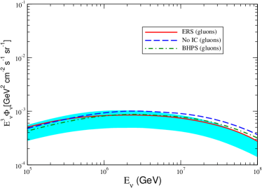
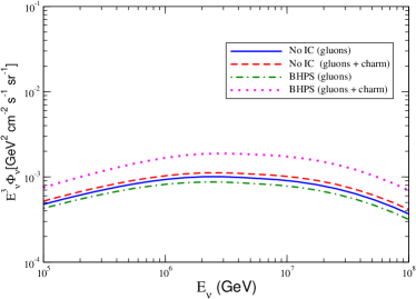
(a)		(b)

Figure 3: Energy dependence of the prompt neutrino flux, normalized by a factor $E_{\nu}^{3}$. (a) Comparison of our predictions with the results obtained in Refs. ers ; enb_stasto2 using the color dipole approach. The results derived in enb_stasto2 considering different phenomenological saturation models for the dipole - proton scattering amplitude are represented by the cyan band. (b) Comparison of the No IC and BHPS predictions considering the gluon and charm contributions and only the gluon one in the calculation of the $x_{F}$ distribution.

Initially, let’s consider that the primary proton flux is described by a broken power-law spectrum. Our motivation to assume this model is associated to the fact that previous estimates for the prompt neutrino flux ers ; enb_stasto2 , which we would like compare our results, has been obtained using this model. In Fig. 3 we present our predictions for the energy dependence of the prompt atmospheric neutrino flux, normalized by a factor $E_{\nu}^{3}$. In the left panel, we compare our predictions with those obtained in Refs. ers ; enb_stasto2 using the color dipole approach and different phenomenological models based on saturation physics. The predictions obtained in Ref. ers are denoted by ERS and those derived in Ref. enb_stasto2 by the cyan band. As in Refs. ers ; enb_stasto2 only the processes initiated by gluon were taken into account, here, for the sake of comparison, we present our predictions derived considering only this channel as well. At low energies ($E_{\nu}\leq 10^{6}$ GeV), the ERS and No IC predictions are very similar. On the other hand, at large energies ($E_{\nu}\geq 10^{7}$ GeV), the No IC predictions imply a larger prompt neutrino flux than that derived in Refs. ers ; enb_stasto2 . Such behavior can be attributed to the model of the dipole - proton scattering amplitude used in our calculations, which differs from those used in Refs. ers ; enb_stasto2 . As demonstrated e.g. in Ref. betemps , the BUW model predicts a slower transition between the linear and non - linear regimes of the QCD dynamics than e.g. the IIM-S one IIM ; Soyez used in Refs. ers ; enb_stasto2 . Consequently, the BUW model implies a faster growth of the heavy quark cross section with the energy, which has direct impact on the prompt neutrino flux at high energies. On the other hand, if the gluon distribution associated to the BHPS parametrization is used as input in the calculations, we find that the resulting predictions are suppressed in comparison to the No IC one. As discussed before, in the BHPS parametrization the IC component is taken into account and this implies that a larger amount of the proton momentum is carried by the charm quarks. Due to the momentum sum rule, the amount carried by the other partons, in particular the gluons, will be reduced. Therefore, the gluon distributions associated to the parton parametrizations which include an intrinsic component are, in general, smaller than those derived disregarding this component [See Fig. 2 (a)]. Such reduction explains the result observed in the left panel of Fig. 3.

In Fig. 3 (b) we estimate the impact of the charm initiated processes on the energy dependence of the prompt neutrino flux. As expected, the inclusion of this new channel of charm production leads to an enhancement of the flux. The magnitude of this enhancement depends on the details of the model of the charm distribution. When the intrinsic charm component is disregarded [the No IC (gluons + charm) curve in Fig. 3] the impact of the charm initiated processes is small. Such result is expected, since the magnitude of the extrinsic charm distribution for small values of $\mu^{2}$ is small. On the other hand, if the intrinsic component is taken into account, we have a large enhancement of the prompt flux.

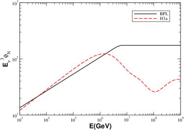
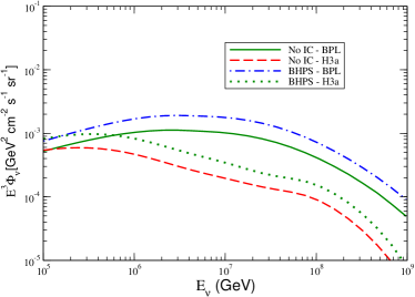
(a)		(b)

Figure 4: (a) Comparison between the BPL and H3a models for the all - nucleon primary cosmic ray spectra. (b) Energy dependence of the prompt neutrino flux, normalized by a factor $E_{\nu}^{3}$, obtained using the BPL and H3a models as input in the calculations.

One important question is the dependence of our results on the model assumed for the primary nucleon spectrum. Although the broken power - law (BPL) approximation of the cosmic ray nucleon flux has been used to evaluate the prompt neutrino flux in almost all early references, more recent publications also present the predictions obtained considering a modern description of the primary spectrum proposed by Gaisser in Ref. gaisser . In what follows we also will estimate the prompt flux using the H3a spectrum, which assumes that the spectrum is given by a composition of 3 populations and 5 representative nuclei, with the set of parameters determined by a global fit of the cosmic ray data gaisser . A comparison between the BPL and H3a spectra is performed in Fig. 4 (a). We have that for primary energies in the range $10^{4}\lesssim E\lesssim 10^{6}$ GeV, the H3a spectrum is larger than the BPL one. On the other hand, for $E\gtrsim 10^{6}$ GeV, the H3a spectrum is smaller than the BPL one, and a structure associated to its composition is present. In Fig. 4 (b) we present our predictions for the energy dependence of the prompt neutrino flux obtained using the BPL and H3a models for the primary nucleon flux. As expected from Fig. 4 (a), the H3a predictions are smaller than the BPL one at large neutrino energies. However, our results indicate a large impact of the intrinsic charm also is present if the H3a spectrum is considered.

A more detailed estimate of the contribution of the charm initiated process and the intrinsic charm component is obtained by the analysis of Fig. 5. In Fig. 5 (a) we present our results for the ratio between the flux calculated considering the gluon and charm channels ($\Phi_{g+c}$) and that derived assuming only the gluon channel ($\Phi_{g}$). The results associated to the BPL and H3a models are presented for comparison. When the IC component is absent, the impact of the charm channel is $\approx 10\%$ and almost energy independent. In contrast, if an IC component is present, the impact increases with the neutrino energy and becomes larger than $200\%$ at large energies, with the H3a predictions being slightly larger than BPL one for $E_{\nu}\lesssim 10^{7}$ GeV. Another way to estimate the impact of the IC component is to calculate the ratio between the flux derived assuming the presence of this component ($\Phi_{BHPS}$) and the flux calculated disregarding this component ($\Phi_{NoIC}$). The results are presented in Fig. 5 (b). They indicate that if only the gluon channel is considered, the presence of the IC component implies a reduction of the prompt neutrino flux of $\approx 10\%$. On the other hand, when the charm channel is included, we predict an enhancement of $\approx 160\%$ in the flux. These results strongly suggest that a generalized treatment of heavy quark production, taking into account charm initiated processes, is crucial to obtain realistic predictions of the prompt flux using the color dipole approach, especially if an intrinsic charm component is present in the proton wave function.

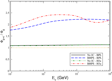
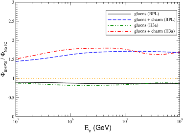
(a)		(b)

Figure 5: Energy dependence of the ratios between prompt neutrino fluxes. (a) Ratio between the flux calculated considering the gluon and charm channels ($\Phi_{g+c}$) and that derived assuming only the gluon channel ($\Phi_{g}$). (b) Ratio between the flux derived assuming the presence of this component ($\Phi_{BHPS}$) with that calculated disregarding this component ($\Phi_{NoIC}$).

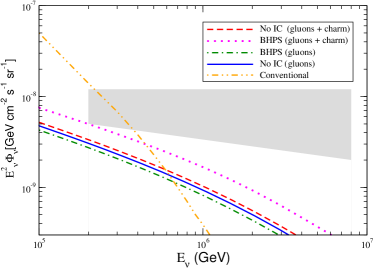
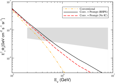
(a)		(b)

Figure 6: Energy dependence of the prompt neutrino flux, normalized by a factor $E_{\nu}^{2}$, obtained considering the BPL model for the primary nucleon spectrum. (a) Comparison of our results with the predictions for the conventional neutrino flux derived in Ref. Honda:2006qj and the astrophysical neutrino flux obtained in Ref. Aartsen:2016xlq , which is represented by the cyan band. (b) Comparison between the predictions for the atmospheric (conventional + prompt) neutrino fluxes and the astrophysical one.

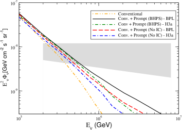
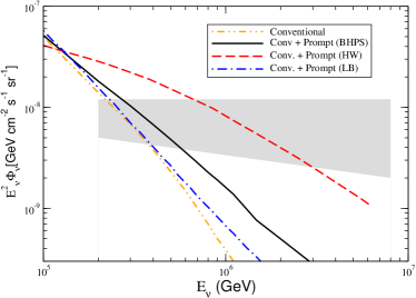
(a)		(b)

Figure 7: (a) Comparison between the BPL and H3a predictions for the energy dependence of the atmospheric (conventional + prompt) neutrino fluxes, normalized by a factor $E_{\nu}^{2}$. (b) Comparison between the BHPS predictions for the atmospheric (conventional + prompt) neutrino flux with the results derived by Halzen and Willie (HW) halzen and by Laha and Brodsky (LB) laha . Results derived using the H3a spectrum.

Using its six-year experimental data, the ICECUBE Collaboration has recently Aartsen:2016xlq estimated the astrophysical neutrino spectrum with the help of an unbroken power - law model. In order to compare our predictions with the neutrino flux derived in Ref. Aartsen:2016xlq , in Fig. 6 we present our results for the neutrino flux, normalized by a factor $E_{\nu}^{2}$, obtained considering the BPL model for the primary nucleon spectrum. The results from Ref. Aartsen:2016xlq are represented by the gray band. For the sake of comparison, we also present the predictions for the conventional atmospheric neutrino flux derived in Ref. Honda:2006qj . In Fig. 6 (a) we compare our predictions for the prompt neutrino flux, considering different models and channels, with the conventional and astrophysical predictions. When the IC component and/or the charm channel is disregarded, the prompt contribution dominates for $E_{\nu}\gtrsim 6\times 10^{5}$ GeV. On the other hand, if the IC component and the charm channel are taken into account, this transition occurs at $E_{\nu}\gtrsim 4.5\times 10^{5}$ GeV. The most important aspect is that, although the astrophysical neutrino flux is dominant at large energies, the magnitude of the background associated to the prompt flux is strongly dependent on the presence or absence of the intrinsic component in the proton wave function, in agreement with the result obtained in Ref. laha . This dependence is more visible in the right panel of Fig. 6, where we present our predictions for the sum of the conventional and prompt fluxes and compare them with the ICECUBE results for the astrophysical neutrino flux. We observe that the inclusion of the IC component leads to an enhancement of the atmospheric (conventional + prompt) neutrino flux of $\approx 45\%$ at $E_{\nu}=10^{6}$ GeV and of $\approx 200\%$ at $E_{\nu}=3.5\times 10^{6}$ GeV. Such large values are in agreement with the expectation discussed in Ref. prdnos .

In Fig. 7 (a) we compare the BPL predictions with those obtained using the H3a model for the primary nucleon spectrum. As expected from our previous analysis, the atmospheric (conventional + prompt) neutrino flux derived using the H3a model is smaller the BPL one at large neutrino energies and they are similar to $E_{\nu}\approx 10^{5}$ GeV. Finally, in Fig. 7 (b) we compare the BHPS predictions, derived using the H3a spectrum, with the corresponding results obtained in Refs. halzen ; laha , considering different assumptions for the intrinsic charm component. In particular, in Ref. halzen the authors have derived an upper limit for the neutrino spectrum assuming a maximum value for the contribution associated to the hadronization of the spectator charm with the valence quarks of projectile. This upper limit is denoted by HW in the figure. On the other, in Ref. laha (denoted LB hereafter) the normalization of the intrinsic charm contribution for the $x_{F}$ - distribution is constrained by the data at low energies presented by the ISR experiments and LEBC - MPS Collaboration, with the energy dependence being that of the inelastic $pp$ cross section (See Ref. laha for details). We have that our predictions are below from the BW one at large energies, with the difference between the results increasing with the neutrino energy. On the other hand, we predict a larger atmospheric neutrino flux than the LB model in the range probed by the IceCube. We believe that this difference is mainly associated to the energy dependence of the intrinsic contribution, which in our calculations is steeper than the energy dependence of the inelastic $pp$ cross section. As a consequence, our contribution of the charm initiated process increases faster with the center - of - mass energy than the LB one. The discrimination between these different predictions can, in principle, be feasible by future IceCube measurements dedicated to contrain the magnitude of the prompt contribution.

At this point, some comments are in order. In our calculations we have considered only the BHPS model of intrinsic charm, in which the amount of IC is maximal. From the results presented in Ref. prdnos , we can expect that if the Meson Cloud model is considered, we will get similar results for the enhancement associated to the IC component. However, if the amount of momentum carried by the IC component is reduced, this will change our predictions for the prompt neutrino flux. Therefore, our predictions should be considered as an upper limit for the impact of the IC component. Another important aspect that should be emphasized is that we have used the color dipole approach to estimate the prompt neutrino flux. As discussed in detail in Refs. enb_stasto2 ; vicantoni , this model implies a $x_{F}$ - distribution that is larger at intermediate values of $x_{F}$ than those obtained with the collinear and with the $k_{T}$ - factorization formalisms. As explained in Refs. enb_stasto2 ; vicantoni , such behavior is somewhat unexpected as this approach includes saturation effects that should lead rather to a reduction of the cross section compared to the collinear and the $k_{T}$ factorization approaches. The explanation of this difference is still an open question and theme of debate (For a more detailed discussion see Ref. vicantoni ). Consequently, the color dipole predictions should be considered as upper bounds for the prompt neutrino flux. The mentioned aspects imply that our predictions should be considered as upper bounds. However, we believe that our results strongly indicate that the inclusion of the charm channel in the color dipole approach for the heavy quark production is important to obtain realistic predictions and that the prompt neutrino flux is sensitive to the presence or absence of an IC component in the hadron wave function.

IV Summary

A complete knowledge of the partonic structure of hadrons is fundamental to make predictions for the Standard Model and beyond Standard Model processes observed at hadron colliders. In particular, the heavy quark component of the proton has a direct impact on the calculation of the prompt atmospheric neutrino flux, which is a background to the astrophysical neutrino flux measured by the ICECUBE Collaboration. One important (and not yet known) quantity for heavy quark production is the amount of the intrinsic component in the hadron wave function. It carries a large fraction of the hadron momentum and, consequently, is expected to modify the cross sections and associated distributions of the produced heavy quarks and heavy mesons at forward rapidities. In this paper we have estimated the impact of the intrinsic charm component on the prompt neutrino flux using the color dipole approach to compute the charm $x_{F}$ - distribution. Following Ref. prdnos , we have generalized previous color dipole calculations by taking into account the contribution of processes initiated by charm quarks. Moreover, differently from previous studies of IC effects, we have used in our calculations the parton distributions derived from the global analysis of a large set of experimental data, with evolution described by the DGLAP equations. Additionally, we have used as input in our calculations a model for the dipole - proton scattering amplitude that describes very well particle production at forward rapidities and LHC energies. Our results indicate that the inclusion of the channel initiated by charm quarks has a strong effect on the prompt neutrino flux. In particular, if an IC component is present in the hadron wave function, our results indicate that the flux is enhanced by a factor 2 at large neutrino energies. Furthermore, we find that the astrophysical neutrino flux becomes dominant at $E_{\nu}\approx 10^{6}$ GeV. However, the magnitude of the background is strongly sensitive to the description of the prompt neutrino flux. Consequently, in order to disentangle the magnitude of the astrophysical contribution to the neutrino flux, it is mandatory to have a better theoretical and experimental control of the prompt neutrino flux.

References

- (1) M. G. Aartsen et al. [IceCube Collaboration], Science 342, 1242856 (2013).
- (2) M. G. Aartsen et al. [IceCube Collaboration], Phys. Rev. Lett. 113, 101101 (2014).
- (3) M. G. Aartsen et al. [IceCube Collaboration], Astrophys. J. 833, 3 (2016).
- (4) T. Gaisser and F. Halzen, Ann. Rev. Nucl. Part. Sci. 64, 101 (2014).
- (5) P. Meszaros, Ann. Rev. Nucl. Part. Sci. 67, 45 (2017)
- (6) R. Abbasi et al. [IceCube Collaboration], Phys. Rev. D 83, 012001 (2011).
- (7) M. G. Aartsen et al. [IceCube Collaboration], Phys. Rev. Lett. 110, 151105 (2013).
- (8) P. Adamson et al. [MINOS Collaboration], Phys. Rev. D 86, 052007 (2012).
- (9) Y. Fukuda et al. [Super-Kamiokande Collaboration], Phys. Lett. B 436, 33 (1998).
- (10) M. Honda, T. Kajita, K. Kasahara, S. Midorikawa and T. Sanuki, Phys. Rev. D 75, 043006 (2007).
- (11) G. D. Barr, T. K. Gaisser, P. Lipari, S. Robbins and T. Stanev, Phys. Rev. D 70, 023006 (2004).
- (12) T. K. Gaisser and S. R. Klein, Astropart. Phys. 64, 13 (2015).
- (13) P. Gondolo, G. Ingelman and M. Thunman, Astropart. Phys. 5, 309 (1996).
- (14) A. D. Martin, M. G. Ryskin and A. M. Stasto, Acta Phys. Polon. B 34, 3273 (2003).
- (15) M. V. Garzelli, S. Moch and G. Sigl, JHEP 1510, 115 (2015).
- (16) A. Bhattacharya, R. Enberg, M. H. Reno, I. Sarcevic and A. Stasto, JHEP 1506, 110 (2015).
- (17) R. Gauld, J. Rojo, L. Rottoli and J. Talbert, JHEP 1511, 009 (2015).
- (18) A. Bhattacharya, R. Enberg, Y. S. Jeong, C. S. Kim, M. H. Reno, I. Sarcevic and A. Stasto, JHEP 1611, 167 (2016).
- (19) R. Gauld, J. Rojo, L. Rottoli, S. Sarkar and J. Talbert, JHEP 1602, 130 (2016).
- (20) F. Halzen and L. Wille, Phys. Rev. D 94, 014014 (2016).
- (21) R. Laha and S. J. Brodsky, Phys. Rev. D 96, 123002 (2017)
- (22) M. V. Garzelli et al. [PROSA Collaboration], JHEP 1705, 004 (2017).
- (23) M. Benzke, M. V. Garzelli, B. Kniehl, G. Kramer, S. Moch and G. Sigl, JHEP 1712, 021 (2017).
- (24) R. Aaij et al. [LHCb Collaboration], Nucl. Phys. B 871, 1 (2013).
- (25) R. Aaij et al. [LHCb Collaboration], JHEP 1603, 159 (2016); Erratum: [JHEP 1609, 013 (2016)]; Erratum: [JHEP 1705, 074 (2017)].
- (26) V. P. Goncalves, R. Maciula, R. Pasechnik and A. Szczurek, Phys. Rev. D 96, 094026 (2017)
- (27) D. Kharzeev and K. Tuchin, Nucl. Phys. A 735, 248 (2004).
- (28) K. Tuchin, Phys. Lett. B 593, 66 (2004); Nucl. Phys. A 798, 61 (2008); Y. V. Kovchegov and K. Tuchin, Phys. Rev. D 74, 054014 (2006); H. Fujii, F. Gelis and R. Venugopalan, J. Phys. G 34, S937 (2007).
- (29) V. P. Goncalves and M. V. T. Machado, JHEP 0704, 028 (2007).
- (30) E. R. Cazaroto, V. P. Goncalves and F. S. Navarra, Nucl. Phys. A 872, 196 (2011).
- (31) H. Fujii and K. Watanabe, Nucl. Phys. A 920, 78 (2013).
- (32) T. Altinoluk, N. Armesto, G. Beuf, A. Kovner and M. Lublinsky, Phys. Rev. D 93, 054049 (2016).
- (33) F. Gelis, E. Iancu, J. Jalilian-Marian and R. Venugopalan, Ann. Rev. Nucl. Part. Sci. 60, 463 (2010); E. Iancu and R. Venugopalan, arXiv:hep-ph/0303204; H. Weigert, Prog. Part. Nucl. Phys. 55, 461 (2005); J. Jalilian-Marian and Y. V. Kovchegov, Prog. Part. Nucl. Phys. 56, 104 (2006); J. L. Albacete and C. Marquet, Prog. Part. Nucl. Phys. 76, 1 (2014).
- (34) A. Dumitru, A. Hayashigaki and J. Jalilian-Marian, Nucl. Phys. A 765, 464 (2006); Nucl. Phys. A 770, 57 (2006).
- (35) D. Boer, A. Utermann, E. Wessels, Phys. Rev. D 77, 054014 (2008).
- (36) F. O. Durães, A. V. Giannini, V. P. Goncalves and F. S. Navarra, Phys. Rev. C 94, 024917 (2016).
- (37) S. J. Brodsky, A. Kusina, F. Lyonnet, I. Schienbein, H. Spiesberger and R. Vogt, Adv. High Energy Phys. 2015, 231547 (2015).
- (38) S. J. Brodsky, V. A. Bednyakov, G. I. Lykasov, J. Smiesko and S. Tokar, Prog. Part. Nucl. Phys. 93, 108 (2017)
- (39) S. J. Brodsky, P. Hoyer, C. Peterson and N. Sakai, Phys. Lett. B 93, 451 (1980).
- (40) V. D. Barger, F. Halzen and W. Y. Keung, Phys. Rev. D 25, 112 (1982).
- (41) S. Paiva, M. Nielsen, F. S. Navarra, F. O. Duraes and L. L. Barz, Mod. Phys. Lett. A 13, 2715 (1998); F. S. Navarra, M. Nielsen, C. A. A. Nunes and M. Teixeira, Phys. Rev. D 54, 842 (1996).
- (42) F. M. Steffens, W. Melnitchouk and A. W. Thomas, Eur. Phys. J. C 11, 673 (1999).
- (43) P. Jimenez-Delgado, T. J. Hobbs, J. T. Londergan and W. Melnitchouk, Phys. Rev. Lett. 116, 019102 (2016).
- (44) S. J. Brodsky and S. Gardner, Phys. Rev. Lett. 116, 019101 (2016).
- (45) V. A. Bednyakov, M. A. Demichev, G. I. Lykasov, T. Stavreva and M. Stockton, Phys. Lett. B 728, 602 (2014); P. H. Beauchemin, V. A. Bednyakov, G. I. Lykasov and Y. Y. Stepanenko, Phys. Rev. D 92, 034014 (2015).
- (46) G. Bailas and V. P. Goncalves, Eur. Phys. J. C 76, 105 (2016).
- (47) T. Boettcher, P. Ilten and M. Williams, Phys. Rev. D 93, 074008 (2016).
- (48) V. P. Goncalves, F. S. Navarra and T. Ullrich, Nucl. Phys. A 842, 59 (2010).
- (49) B. A. Kniehl, G. Kramer, I. Schienbein and H. Spiesberger, Phys. Rev. D 79, 094009 (2009).
- (50) F. Carvalho, A. V. Giannini, V. P. Goncalves and F. S. Navarra, Phys. Rev. D 96, 094002 (2017)
- (51) R. Enberg, M. H. Reno and I. Sarcevic, Phys. Rev. D 78, 043005 (2008)
- (52) L. Pasquali, M. H. Reno and I. Sarcevic, Phys. Rev. D 59, 034020 (1999)
- (53) N. N. Nikolaev, G. Piller and B. G. Zakharov, J. Exp. Theor. Phys. 81, 851 (1995) [Zh. Eksp. Teor. Fiz. 108, 1554 (1995)]; Z. Phys. A 354, 99 (1996).
- (54) B. Z. Kopeliovich and A. V. Tarasov, Nucl. Phys. A 710, 180 (2002).
- (55) I. Balitsky, Nucl. Phys. B 463, 99 (1996); Y. V. Kovchegov, Phys. Rev. D 60, 034008 (1999); Phys. Rev. D 61, 074018 (2000).
- (56) T. Lappi and H. Mantysaari, Phys. Rev. D 91, 074016 (2015).
- (57) D. Kharzeev, Y.V. Kovchegov and K. Tuchin, Phys. Lett. B599, 23 (2004); J. Bartels, K. Golec-Biernat, H. Kowalski, Phys. Rev. D 66, 014001 (2002); H. Kowalski and D. Teaney, Phys. Rev. D 68, 114005 (2003); H. Kowalski, L. Motyka and G. Watt, Phys. Rev. D 74, 074016(2006); V. P. Goncalves, M. S. Kugeratski, M. V. T. Machado and F. S. Navarra, Phys. Lett. B 643, 273 (2006); C. Marquet, R. Peschanski and G. Soyez, Phys. Rev. D 76, 034011 (2007); G. Watt and H. Kowalski, Phys. Rev. D 78, 014016 (2008).
- (58) E. Iancu, K. Itakura, S. Munier, Phys. Lett. B590, 199 (2004)
- (59) G. Soyez, Phys. Lett. B 655, 32 (2007)
- (60) J. Pumplin, H. L. Lai and W. K. Tung, Phys. Rev. D 75, 054029 (2007).
- (61) M. A. Betemps, V. P. Goncalves and J. T. de Santana Amaral, Eur. Phys. J. C 66, 137 (2010)
- (62) T. K. Gaisser, Astropart. Phys. 35, 801 (2012)
- (63) S. Dulat, T.-J. Hou, J. Gao, J. Huston, J. Pumplin, C. Schmidt et al., Phys. Rev. D 89 073004, (2014).
- (64) J. Raufeisen and J. C. Peng, Phys. Rev. D 67, 054008 (2003)