Instituto de Estudos Avançados Transdisciplinares Universidade Federal de Minas Gerais The origins of the Malagasy people, some certainties and a few mysteries Maurizio Serva¹ Malagasy dialects — Austronesian languages — Lexicostatistics — Malagasy origins The Malagasy language belongs to the Greater Barito East group of the Austronesian family, the language most closely connected to Malagasy dialects is Maanyan (Kalimantan), but Malay as well other Indonesian and Philippine languages are also related. The African contribution is very high in the Malagasy genetic make-up (about 50%) but negligible in the language. Because of the linguistic link, it is widely accepted that the island was settled by Indonesian sailors after a maritime trek but date and place of landing are still debated. The 50% Indonesian genetic contribution to present Malagasy points in a different direction then Maanyan for the Asian ancestry, therefore, the ethnic composition of the Austronesian settlers is also still debated. In this talk I mainly review the joint research of Filippo Petroni, Dima Volchenkov, Sören Wichmann and myself which tries to shed new light on these problems. The key point is the application of a new quantitative methodology which is able to find out the kinship relations among languages (or dialects). New techniques are also introduced in order to extract the maximum information from these relations concerning time and space patterns.

1 Introduction

The Austronesian expansion, which very likely started from Taiwan or from the south of China [Gray and Jordan, 2000, Hurles et al 2005], is probably the most spectacular event of maritime colonization in human history as it can be appreciated in Fig. 1.

The Malagasy language (as well as all its dialects) belongs to the Austronesian linguistic family, as was suggested already in [Houtman, 1603] and later firmly established in [Tuuk, 1864]. Much more recently, Dahl [Dahl, 1951] pointed out a particularly close relationship between Malagasy and Maanyan of south-east Kalimantan, which share about 45% their basic vocabulary [Dyen, 1953]. But Malagasy also bears similarities to languages in Sulawesi, Malaysia, Sumatra and Philippines, including loanwords from Malay, Javanese, and one (or more) language(s) of southern Sulawesi [Adelaar, 2009].

The genetic make-up of Malagasy people exhibits almost equal proportions of African and Indonesian heritage [Hurles et al 2005]. Nevertheless its Bantu component in the vocabulary seems to be very limited and mostly concerns faunal names [Blench and Walsh, 2009].

The history of Madagascar peopling and settlement is subject to alternative interpretations among scholars. It seems that Indonesian sailors reached Madagascar by a maritime trek at a time between one to two thousand years ago (the exact time and the place of landing are still debated) but until recently it was not clear whether there were multiple settlements or just a single one.

This last question was answered in [Cox et al, 2012] were it was shown that Madagascar was settled by a very small group of women (approx. 30). This highly restricted founding population suggests that Madagascar was settled through a single, perhaps even unintended, transoceanic crossing.

Additional questions are raised by the fact that the Maanyan speakers, which live along the rivers of Kalimantan, have not the necessary skills for long-distance maritime navigation. Moreover, recent research on DNA, while pointing to south-east Kalimantan and Sulawesi for the Indonesian ancestry, firmly rejects a direct genetic link between Malagasy and Maanyan. [Kusuma et al, 2015, Kusuma et al, 2016].

In this talk I review our results which give information about the following points:

1. the historical configuration of Malagasy dialects,

2. when the migration to Madagascar took place,

3. how Malagasy is related to other Austronesian languages,

4. where the original settlement of the Malagasy people took place.

Our research addresses these four problems through the application of new quantitative methodologies inspired by, but nevertheless different from, classical lexicostatistics and glottochronology [Serva and Petroni, 2008, Holman et al, 2008, Petroni and Serva, 2008, Bakker et al, 2009].

The data, collected during the beginning of 2010 by one of the authors (M.S.), consist of 200-item Swadesh word lists for 23 dialects of Malagasy from all areas of the island. A practical orthography which corresponds to the orthographic conventions of standard Malagasy has been used. Most of the informants were able to write the words directly using these conventions, while a few of them benefited from the help of one or more fellow townsmen. A cross-checking of each dialect list was done by eliciting data separately from two different consultants. Details about the speakers who furnished the data are in [Serva et al, 2012] while the dataset can be found in [Serva and Petroni, 2011], This dataset probably represents the largest collection available of comparative Swadesh lists for Malagasy (see Fig. 4 for the locations).

While there are linguistic as well as geographical and temporal dimensions to the issues addressed in this talk, all strands of the investigation are rooted in an automated comparison of words. Our automated method (see Appendix A for details) works as follows: for any language we write down a Swadesh list, then we compare words with same meaning belonging to different languages only considering orthographic differences. This approach is motivated by the analogy with genetics: the vocabulary has the role of DNA and the comparison is simply made by measuring the differences between the DNA of the two languages. There are various advantages: the first is that, at variance with previous methods, it avoids subjectivity, the second is that results can be replicated by other scholars assuming that the database is the same, the third is that it is not requested a specific expertize in linguistic, and the last, but surely not the least, is that it allows for a rapid comparison of a very large number of languages (or dialects).

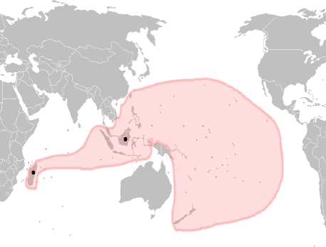
Figure 1: The distribution of Austronesian languages. The black spots indicate Madagascar and Kalimantan, where Maanyan, the closest relative of Malagasy, is spoken.

The first use of the pairwise distances is to derive a classification of the dialects. For this purpose we adopt a multiple strategy in order to extract a maximum of information from the set of pairwise distances. We first obtain a tree representation of the set by using two different standard phylogenetic algorithms, then we adopt a strategy (SCA) which, analogously to a principal components approach, represents the set in terms of geometrical relations. The SCA analysis also provides the tool for a dating of the landing of Malagasy ancestors on the island. The landing area is established assuming that a linguistic homeland is the area exhibiting the maximum of current linguistic diversity. Diversity is measured by comparing lexical and geographical distances. Finally, we perform a comparison of all variants with some other Austronesian languages, in particular with Malay and Maanyan.

For the purpose of comparison of Malagasy variants with other Austronesian languages we draw upon The Austronesian Basic Vocabulary Database. [Greenhill et al, 2009]. Since the wordlists in this database do not always contain all the 200 items of our Swadesh lists they are supplemented by various sources (including the database of the Automated Similarity Judgment Program (ASJP)[Wichmann et al, 2017]) and by author’s interviews.

2 Method

Our strategies [Serva and Petroni, 2008, Holman et al, 2008, Petroni and Serva, 2008, Bakker et al, 2009] are based on a lexical comparison of languages by means of an automated measure of distance between pairs of words with same meaning contained in Swadesh lists. The use of Swadesh lists [Swadesh, 1952] in lexicostatistics has been popular for more than half a century. They are lists of words associated with the same $M$ meanings, (the original choice of Swadesh was $M=200$) which tend (1) to be found in all languages, (2) to be relatively stable, (3) to not frequently be borrowed, and (4) to be basic rather than derived concepts. It has to be stressed that these are tendencies and that convenience play a great part in the way the list of concepts was put together. Still, it has become standard, and here we simply follow Swadesh and the many other scholars who have applied it. Comparing the two lists corresponding to a pair of languages it is possible to determine the percentage of shared cognates which is a measure of their lexical distance. A recent example of the use of Swadesh lists and cognates counting to construct language trees are the studies of Gray and Atkinson [Gray and Atkinson, 2003] and Gray and Jordan [Gray and Jordan, 2000].

The idea of measuring relationships among languages using vocabulary is much older than lexicostatistics and it seems to have its roots in the work of the French explorer Dumont D’Urville. He collected comparative word lists during his voyages aboard the Astrolabe from 1826 to 1829 and, in his work about the geographical division of the Pacific [D’Urville, 1832], he proposed a method to measure the degree of relation among languages. He used a core vocabulary of 115 terms, then he assigned a distance from 0 to 1 to any pair of words with the same meaning and finally he was able to determine the degree of relation between any pair of languages.

Our results are obtained through a specific version of the so-called Levenshtein or ’edit’ distance (henceforth LD) [Levenshtein, 1966]. The version we use here was introduced by [Serva and Petroni, 2008, Petroni and Serva, 2008] and consists of the following procedure. Words referring to the same concept for a given pair of dialects are compared with a view to how easily the word in dialect A is transformed into the corresponding word in dialect B. Steps allowed in the transformations are: insertions, deletions, and substitutions. The LD is then calculated as the minimal number of such steps required to completely transform one word into the other. Calculating the distance measure we use (the ’normalized Levenshtein distance’, or LDN), requires one more operation: the ’raw LD’ is divided by the length (in terms of segments) of the longer of the two words compared. This operation produces LDN values between 0 and 1 and takes into account variable word lengths: if one or both of the words compared happen to be relatively long, the LD is prone to be higher than if they both happen to be short, so without the normalization the distance values would not be comparable. Finally we average the LDN’s for all 200 pairs of words compared to obtain a distance value characterizing the overall difference between a pair of dialects (see Appendix A for a compact mathematical definition and a table with all distances).

Thus, the Levenshtein distance is sensitive to both lexical replacement and phonological change and therefore differs from the cognate counting procedure of classical lexicostatistics even if the results are usually roughly equivalent.

If a family of languages is considered, all the information is encoded in a matrix whose entries are the pairwise lexical distances. But information about the total relationship among the languages is not manifest and it has to be extracted. The ubiquitous approach to this problem is to transform the matrix information in a phylogenetic tree.

Nevertheless, in this transformation, part of the information may be lost because transfer among languages is not exclusively vertical (as in mtDNA transmission from mother to child) but it also can be horizontal (borrowings and, in extreme cases, creolization). Another approach is the geometric one [Blanchard et al, 2010a, Blanchard et al, 2010b] that results from Structural Component Analysis (SCA) that we have recently proposed. This approach encodes the matrix information into the positions of the languages in a $n$-dimensional space. For large $n$ one recovers all the matrix content, but a low dimensionality, typically $n$=2 or $n$=3, is sufficient to grasp all the relevant information. The results presented in this talk mostly rely to a direct investigation of the entries of the matrix and to simple averages over them.

3 Phylogenetic trees and geography

The number of Malagasy dialects we consider is $N$=23, therefore, the output of our method, when applied only to these variants is a matrix with $N(N-1)/2=253$ non-trivial entries representing all the possible lexical distances among dialects. This matrix is explicitly shown in Appendix A.

The information concerning the vertical transmission of vocabulary from proto-Malagasy to the contemporary dialects can be extracted by a phylogenetic approach. There are various possible choices for the algorithm for the reconstruction of the family tree. The two algorithms used are Neighbor-Joining (NJ) [Saitou and Nei, 1987] and the Unweighted Pair Group Method (UPGMA) [Sokal and Michener, 1958]. The main theoretical difference between the algorithms is that UPGMA assumes that evolutionary rates are the same on all branches of the tree, while NJ allows differences in evolutionary rates. The question of which method is better at inferring the phylogeny has been studied by running various simulations where the true phylogeny is known. Most of these studies were in biology but at least one [Barbançon et al, 2006] specifically tried to emulate linguistic data. Most of the studies (starting with [Saitou and Nei, 1987] and including [Barbançon et al, 2006]) found that NJ usually came closer to the true phylogeny. Since in our case, the relations among dialects are not necessarily tree-like, it is desirable to test the different methods against empirical linguistic data, which is mainly why trees derived by means of both methods are presented here.

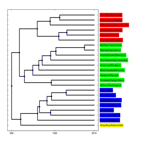
Figure 2: Phylogenetic tree of 23 Malagasy dialects realized by Unweighted Pair Group Method Average (UPGMA). In this figure the name of the dialect is followed by the name of the town were it was collected. The phylogenetic tree shows a partition of the Malagasy dialects into four main groups indicated by different colors.

The input data for the UPGMA tree are the pairwise separation times obtained from lexical distances by a rule [Serva and Petroni, 2008] which is a simple generalization of the fundamental formula of glottochronology. The absolute time-scale is calibrated by the results of the SCA analysis (see below), which indicate a separation date of 650 CE. While the scale below the UPGMA tree (Fig. 2) refers to separation times, the scale below the NJ tree (Fig. 3) simply shows lexical distance from the root. The LDN distance between two language variants is roughly equal to the sum of their lexical distance from their closest common node.

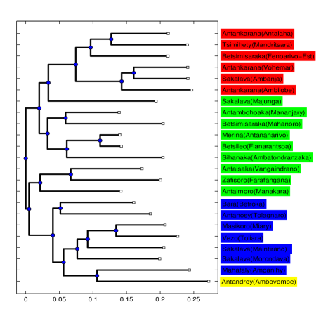
Figure 3: NJ tree for 23 Malagasy dialects. Colors compare with the UPGMA tree in Fig. 2. The graph confirms the main center-north-east vs. south-west division. The main difference is that three dialects at the linguistic border are grouped differently. Colors allows for a rapid comparison.

Since UPGMA assumes equal evolutionary rates, the ends of all the branches line up on the right side of the UPGMA tree. The assumption of equal rates also determines the root of the tree on the left side. NJ allows unequal rates, so the ends of the branches do not all line up on the NJ tree. The extent to which they fail to line up indicates how variable the rates are. The tree is rooted by the midpoint (the point in the network in between the two most distant dialects) but we also checked that the same result is obtained following the standard strategy of adding an out-group.

There is a good fit between the geographical position of dialects (see Fig. 4) and their position both in the UPGMA (see Fig. 2) and NJ trees (see Fig. 3). In both trees the dialects are divided into two main groups (colored blue and yellow vs. red and green in Fig. 2).

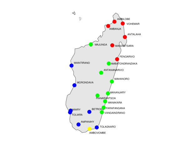
Figure 4: Geography of Malagasy dialects. The locations of the 23 dialects are indicated with the same colors of Fig. 2. Any dialect is identified by the the name of the town where it was collected.

Given the consensus between the two methods, the result regarding the basic split can be considered solid. Geographically the division corresponds to a border running from the south-east to the north-west of the island, as shown in Fig. 4 where the UPGMA and NJ main separation lines are drawn. A major difference concerns the Vangaindrano, Farafangana and Manakara dialects, which have shifting allegiances with respect to the two main groups under the different analyses. Additionally, there are minor differences in the way that the two main groups are configured internally. Most strikingly, we observe that in the UPGMA tree Majunga (a.k.a. Mahajanga) is grouped with the central dialects while in the NJ tree it is grouped with the northern ones. This indeterminacy would seem to relate to the fact that the town of Majunga is at the geographical border of the two regions.

Another difference is that in the UPGMA tree the Ambovombe variant of the dialect traditionally called Antandroy is quite isolated, whereas in the NJ tree Ambovombe and the Ampanihy variant of Mahafaly group together. Since the UPGMA algorithm is a strict bottom-up approach to the construction of a phylogeny, where the closest taxa a joined first, it will tend to treat the overall most deviant variant last. In contrast, the NJ algorithm privileges pairwise similarities. This explains the differential placement of Ambovombe in the two trees.

The length of the branch leading to the node that joins Ambovombe and Ampanihy in the NJ tree shows that these two variants have quite a lot of similarities but in the UPGMA method these similarities in a sense ’drown’ in the differences that set Ambovombe off from other Malagasy variants as a whole.

The phylogenetic trees interestingly shows a main partition of Malagasy dialects in two main branches (east-center-north and south-west) at variance with a previous study which gave a different partitioning [Vérin et al, 1969] isolating northern dialects (indeed, results in [Vérin et al, 1969] coincide with ours if a modern phylogenetic algorithm is applied to their data, see [Serva et al, 2012] for a discussion of this point.)

4 Structural Component Analysis

Although tree diagrams have become ubiquitous in representations of language taxonomies, they fail to reveal the full complexity of affinities among languages. The reason is that the simple relation of ancestry, which is the single principle behind a branching family tree model, cannot grasp the complex social, cultural and political factors molding the evolution of languages [Heggarty, 2006]. Since all dialects within a group interact with each other and with the languages of other families in ’real time’, it is obvious that any historical development in languages cannot be described only in terms of pair-wise interactions, but reflects a genuine higher order influence, which can best be assessed by Structural Component Analysis (SCA). This is a powerful tool which represents the relationships among different languages in a language family geometrically, in terms of distances and angles, as in the Euclidean geometry of everyday intuition. Being a version of the kernel PCA method [Schölkopf et al, 1998], it generalizes PCA to cases where we are interested in principal components obtained by taking all higher-order correlations between data instances. It has so far been tested through the construction of language taxonomies for fifty major languages of the Indo-European and Austronesian language families [Blanchard et al, 2010a]. The details of the SCA method are given in the Appendix B.

In Fig. 5 we show the three-dimensional geometric representation of 23 dialects of the Malagasy language and the Maanyan language, which is closely related to Malagasy. The three-dimensional space is spanned by the three major data traits ($\{q_{2},q_{3},q_{4}\}$, see Appendix B for details) detected in the matrix of linguistic LDN distances.

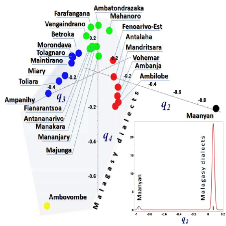
Figure 5: The three-dimensional geometric representation of the Malagasy dialects and the Maanyan language in the space of major data traits ($q_{2},q_{3},q_{4}$) shows a remarkable geographic patterning separating the northern (red) and the southern (blue) dialect groups, which fork from the central part of the island (the dialects spoken in the central part are colored green, while Antandroy is yellow). The kernel density estimate of the distribution of the $q_{2}$ coordinates, together with the absolute data frequencies, indicate that all Malagasy dialects belong to a single plane orthogonal to the data trait of the Maanyan language ($q_{2}$).

The clear geographic patterning is perhaps the most remarkable aspect of the geometric representation. The structural components reveal themselves in Fig. 6 as two well-separated spines representing both the northern (red) and the southern (blue) dialects of entire language.

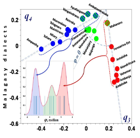
Figure 6: The plane of Malagasy dialects ($q_{3},q_{4}$); Antandroy (Ambovombe) is excluded. The kernel density estimate of the distribution over azimuth angles, together with the absolute data frequencies, allows the rest of Malagasy dialects to be classified into the three groups: north (red), south-west (blue), and center (green).

It is remarkable that all Malagasy dialects belong to a single plane orthogonal to the data trait of the Maanyan language ($q_{2}$). The plane of Malagasy dialects is attested by the sharp distribution of the language points in Cartesian coordinates along the data trait $q_{2}.$ This color point of Malagasy dialects over their common plane is shown in Fig. 7 where a reference azimuth angle $\varphi$ is introduced in order to underline the evident symmetry. It is important to mention that although the language point of Antandroy (Ambovombe) is located on the same plane as the rest of Malagasy dialects, it is situated far away from them and obviously belongs to neither of the dialect branches and for this reason is not reported in next Fig. 7. This clear SCA isolation of Antrandroy is compatible with its position in the tree in Fig. 2.

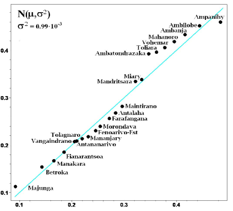
Figure 7: The radial coordinates are ranked and then plotted against their expected values under normality. Departures from linearity, which signify departures from normality, is minimal.

The distribution of language points supports the main conclusion following from the UPGMA and NJ methods (Figs. 1-2) of a division of the main group of Malagasy dialects into three groups: north (red), south-west (blue) and center (green). These clusters are clearly evident from the representation shown in Fig. 7. However, with respect to the classification of some individual dialects the SCA method differs from the UPGMA and NJ results. Since their azimuthal coordinates better fit the general trend of the southern group, the Vangaindrano, Farafangana, and Ambatontrazaka dialects spoken in the central part of the island are now grouped with the southern dialects (blue) rather than the central ones . Similarly, in accordance with the representation shown in Fig. 7, the Mahanoro dialect is now classified in the northern group (red), since it is best fitted to the northern group azimuth angle. The remaining five dialects of the central group (green colored) are characterized by the azimuth angles close to a bisector ($\varphi=0$).

5 A date for landing

The radial coordinate of a dialect is simply the distance of its representative point from the origin of coordinates in Fig. 5. It can be verified that the position of Malagasy dialects along the radial direction is remarkably heterogeneous indicating that the rates of change in the Swadesh vocabulary was anything but constant.

The radial coordinates have been ranked and then plotted in Fig. 7 against their expected values under normality, such that departures from linearity signify departures from normality. The dialect points in Fig. 7 show very good agreement with univariate normality with the value of variance $\sigma^{2}=0.99\times 10^{-3}$ which results from the best fit of the data. This normal behavior can be justified by the hypothesis that the dialect vocabularies are the result of a gradual and cumulative process into which many small, independent innovations have emerged and contributed additively.

In the SCA method, which is based on the statistical evaluation of differences among the items of the Swadesh list, a complex nexus of processes behind the emergence and differentiation of dialects is described by the single degree of freedom (as another degree of freedom, the azimuth angle, is fixed by the dialect group) along the radial direction [Blanchard et al, 2010b].

The univariate normal distribution (Fig. 7) implies a homogeneous diffusion time evolution in one dimension, under which variance $\sigma^{2}\propto t$ grows linearly with time. The locations of dialect points could not be distributed normally if in the long run the value of variance $\sigma^{2}$ did not grow with time at an approximately constant rate. We stress that the constant rate of increase in the variance of radial positions of languages in the geometrical representation (Fig. 5) has nothing to do with the traditional glottochronological assumption about the constant replacement rate of cognates assumed by the UPGMA method.

It is also important to mention that the value of variance $\sigma^{2}=0.99\times 10^{-3}$ calculated for the Malagasy dialects does not correspond to physical time but rather gives a statistically consistent estimate of age for the group of dialects. In order to assess the pace of variance changes with physical time and to calibrate the dating method we have used historically attested events. Although the lack of documented historical events makes the direct calibration of the method difficult, we suggest (following [Blanchard et al, 2010a]) that variance evaluated over the Swadesh vocabulary proceeds approximately at the same pace uniformly for all human societies involved in trading and exchange. For calibrating the dating mechanism in [Blanchard et al, 2010a], we have used the following four anchoring historical events (see [Fouracre:2007]) for the Indo-European language family: i.) the last Celtic migration (to the Balkans and Asia Minor) (by 300 BCE); ii.) the division of the Roman Empire (by 500 CE); iii.) the migration of German tribes to the Danube River (by 100 CE); iv.) the establishment of the Avars Khaganate (by 590 CE) causing the spread of Slavic people. It is remarkable that all of the events mentioned uniformly indicate a very slow variance pace of a millionth per year, $t/\sigma^{2}=(1.367\pm 0.002)\cdot 10^{6}.$ This time-age ratio returns $t=1,353$ years if applied to the Malagasy dialects, suggesting that landing in Madagascar was around 650 CE. This is in complete agreement with the prevalent opinion among scholars including the influential one of Adelaar [Adelaar, 2009].

6 The place of landing

In order to hypothetically infer the original center of dispersal of Malagasy variants, we here use a variant of the method of [Wichmann et al, 2010a]. This method draws upon a well-known idea from biology [Vavilov, 1926] and linguistics [Sapir, 1916] that the homeland of a biological species or a language group corresponds to the current area of greatest diversity. In [Wichmann et al, 2010a] this idea is transformed into quantifiable terms in the following way. For each language variant a diversity index is calculated as the average of the proportions between linguistic and geographical distances from the given language variant to each of the other language variants (cf. [Wichmann et al, 2010a] for more detail). The geographical distance is defined as the great-circle distance (i.e., as the crow flies) measured by angle radians.

In our work we adopted a variant of the method described in more detail in Appendix C. The are two rationales for this variant, the first is that it avoids technical and theoretical problems with pairs of dialects which have a coinciding or a very close geographical location, the second is that it uses the proper scaling proportions between lexical and geographical distances, extrapolated by linear regression.

The result of applying this method to Malagasy variants is that the best candidate for the homeland is the south-east coast where the three most diverse towns, i.e., Farafangana, Mahanoro and Ambovombe, are located, and where the surrounding towns are also highly diverse. The northern locations are the least diverse and they must have been settled last.

A convenient way of displaying the results on a map is shown in Fig. 8, where locations are indicated by means of circles with different gradations of the same color (green). The higher the diversity index of a location is, the darker the color. The figure suggest that the landing would have occurred somewhere between Mahanoro (central part of the east cost) and Ambovobe (extreme south of the east coast), the most probable location being in the center of this area, where Farafangana is situated. Finally, we have checked that if the entire Greater Barito East group is considered, the homeland of Malagasy stays in the same place, but becomes secondary with respect to the southern Kalimantan homeland of the group.

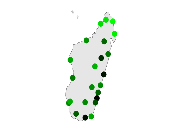
Figure 8: The homeland of Malagasy dialects as determined through diversity measures. The darkest-colored towns have the highest diversity values while the light-colored the lowest. The most diverse area is the south-east coast where landing occurred, the less diverse area in the north, indicating that this area was settled last.

The identification of a linguistic homeland for Malagasy on the south-east coast of Madagascar receives some independent support from unexpected kinds of evidence. According to [Faublée, 1983] there is an Indian Ocean current that connects Sumatra with Madagascar. When Mount Krakatoa exploded in 1883, pumice was washed ashore on Madagascar’s east coast where the Mananjary River opens into the sea (between Farafangana and Mahanoro). During World War II the same area saw the arrival of pieces of wreckage from ships sailing between Java and Sumatra that had been bombed by the Japanese air-force. The mouth of the Mananjary River is where the town of Manajary is presently located, and it is in the highly diverse south-east coast as shown in Fig. 8. To enter the current that would eventually carry them to the east coast of Madagascar the ancestors of today’s Malagasy people would likely have passed by the easily navigable Sunda strait.

In his studies on the roots of Malagasy, Adelaar finds that the language has an important contingent of loanwords from Sulawesi (Buginese). We also have compared Malagasy (and its dialects) with various Indonesian languages (Maanyan, Ngaju Dayak, Javanese, Iban, Banjarese, Bahasa Indonesia Malay, Manguidanaon, Maranao, Makassar, Buginese). While we unsurprisingly find that Maanyan is the closest language, we also find that Buginese is the third closest one (see also [Petroni and Serva, 2008]). The similarity with Buginese appears to be a further argument in favor of the southern path through the Sunda strait to Madagascar. If the correct scenario is one of Malay sailors recruiting a crew of other Austronesians and if the latter were recruited in Kalimantan and, to a limited extent, in Sulawesi, then the settlers likely crossed this strait before starting their navigation in the open waters.

As a further confirmation of this analysis, we also computed the average LDN distance from each dialect to all the others (see Fig. 9).

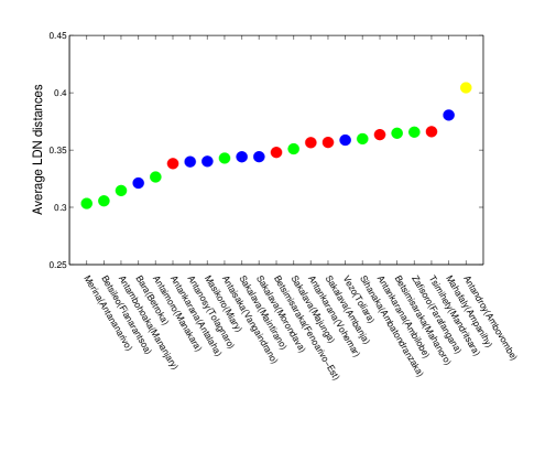
Figure 9: Average LDN distance of each of the dialects from all the others. Colors are chosen according to Figs. 2-3. Highland dialects (Antananarivo, Fianarantsoa and Betroka) together with south-east coast dialects (Mananjary and Manakara) show the smallest average distance.

Antandroy has the largest average distance, confirming that it is the overall most deviant variant (something which is also commonly pointed out by other Malagasy speakers). We further note that the smallest average distance is for Merina (official language), Betsileo and Bara, which are all spoken in the highlands. The fact that Merina has the smallest average distance is possibly partially explained by the fact that this variant is the official one. However, as we will show later by means of a comparison of Malagasy dialects with Malay and Maanyan, this cannot be the only explanation. More interestingly we remark that the Antambohoaka and Antaimoro variants, which are spoken in Mananjary and Manakara, also have a very small average distance from the other dialects. Both dialects are spoken in the south-east coast of Madagascar in a relatively isolated position and, therefore, this is further evidence for south-east as the homeland of the Malagasy language and, likely, as the location of the first settlement.

7 Dialects, Malay and Maanyan

The classification of Malagasy (together with all its dialects) among the Greater Barito East languages of Kalimantan as well as the particularly close relationship with Maanyan established in [Dahl, 1951] is beyond doubt. However, Malagasy also underwent influences from other Indonesian languages such as Malay, Ngaju, Javanese, south-Sulawesi and south-Philippines languages [Adelaar, 1995a, Adelaar, 2009].

The main open problem concerning Malagasy is to determine the composition of the population which settled the island. Adelaar writes : Malay influence persisted for several centuries after the migration. But, except for this Malay influence, most influence on Malagasy from other Indonesian languages seems to be pre-migratory. (…) I also believe it possible that the early migrants from south-east Asia came not exclusively from the south-east Barito area, in fact, that south-east Barito speakers may not even have constituted a majority among these migrants, but rather formed a nuclear group which was later reinforced by south-east Asian migrants with a possibly different linguistic and cultural background (and, of course, by African migrants). Whatever view one may hold on how the early Malagasy were influenced by other Indonesians, it seems necessary that we at least develop a more cosmopolitan view on the Indonesian origins of the Malagasy. A south-east Barito origin is beyond dispute, but this is of course only one aspect of what Malagasy dialects and cultures reflect today. Later influences were manifold, and some of these influences, African as well as Indonesian, were so strong that they have molded the Malagasy language and culture in all its variety into something new, something for the analysis of which a south-east Barito origin has become a factor of little explanatory value.

In order to clarify the problem raised by Adelaar, it is necessary to understand the Malagasy relationships with other Indonesian languages (and possibly African ones). The fact that the use of some words is limited to one or more dialects was already taken into account in previous studies. For example it is known that the word alika which refers to dog in Merina (the official variant) is replaced by the word amboa of Bantu origin in most dialects. Nevertheless, the study of Malagasy dialects in comparison with Indonesian languages is a still largely unexplored field of research. Each dialect may provide pieces of information about the history the language, eventually allowing us to for track the various linguistic influences experienced by Malagasy since the initial colonization of the island. We know that Maanyan is one of the closest Indonesian language to Malagasy while we also know that Malay somehow influenced Malagasy both before and after colonization. In fact, there is also a possibility that the first colonizers were a mixed equipage of Malay seafarers and subordinates speaking en earlier form of Maanyan or a language closely to it, and that Malay influence continued for centuries (the first Malagasy alphabet in Arabic characters was probably introduced by Muslim Malay seafarers). For this reason we have computed the LDN distances of Malagasy dialects from Maanyan and Malay and we show them on the associated Cartesian plane (Fig. 10).

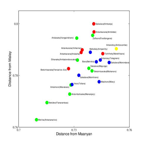
Figure 10: Lexical distances of Malagasy dialects from Malay and Maanyan. Colors are chosen according to Figs. 2-3. Highland dialects together with south-east coast Mananjary and Manakara dialects show the smallest distance from both the two Indonesian languages.

If we consider the 23 dialects together with Malay and Maanyan, not only do we have to compute the 253 internal distances, but also we have to determine the 23x2=56 distances of any of the dialects from the two Indonesian languages. These new distances are displayed in Fig. 10.

First of all we observe, as expected, that the largest of the distances from Maanyan is smaller then the smallest of the distances from Malay. This simply reflects the fact that Malagasy is first of all an East Barito language. Then we also observe that Malagasy dialects seem to have almost the same relative composition. In fact, all the points in Fig. 10 have almost the same distance from Malay/distance from Maanyan ratio. This is a strong indication that the linguistic makeup is substantially the same for all dialects and, therefore, that they all originated by the same founding population of which they reflect the initial composition. The conclusion is that the founding event was likely a single one ([Cox et al, 2012])and subsequent immigration did not significantly alter the linguistic composition.

Indeed, looking more carefully, one can detect a little less Malay in the north since red circles have a larger ratio with respect all the others. This cannot a be a consequence of a larger African influence in the vocabulary due to the active trade with the continent and Comoros islands. In this case both the Maanyan and Malay component of the vocabulary would be affected. Instead, this may be the effect of Malay trading which, according to Adelaar, continued for several centuries after colonization.

Noticeably, some dialects changed less with respect to the proto-language (Antananarivo, Fianarantsoa, Manajary, Manakara), in fact, their distances both from Maanyan and Malay are smaller then those of the other dialects. This is probably the most relevant phenomenon, and we underline that the variants which are less distant on average with respect to the other dialects (Fig. 9) are also less distant with respect to Malay and Maanyan (Fig. 10). Therefore, the fact that Merina is closer to the other dialects cannot be merely justified by the fact that it is the official variant.

We have checked whether the picture which emerges from Fig. 10 is confirmed by comparing with other related Indonesian languages. The result is positive, and in particular the dialects of Manajary, Manakara, Antananarivo and Fianarantsoa seem to be closer to most of the Indonesian languages which we compare them to. Note that Manajary and Manakara are both in the previously identified landing area on the south-east coast while Antananarivo and Fianarantsoa are in the central highlands of the island. This suggests a scenario according to which there was a migration to the highlands of Madagascar (Betsileo and Imerina regions) shortly after the landing on the south-east coast (Manakara, Manajary).

In conclusion, both average distances in Fig. 9 and distances from related Indonesian language (Fig. 10) point to the south-east coast as the area of the first settlement. This is the same indication which comes from the fact that linguistic diversity is higher in that region.

Finally, we remark that the Antandroy variant (Ambovombe-be) is the most distant from Maanyan and among the most distant dialects from Malay, again showing itself to be the most deviant dialect. It is not clear whether its divergent evolution was due to internal factors or to specific language contacts which are still to be identified.

8 Certainties and mysteries

All results presented in this talk rely on two main ingredients: a new dataset from 23 different variants of the languages (plus Malay and Maanyan) and an automated method to evaluate lexical distances. Analyzing the distances through different types of phylogenetic algorithm (NJ and UPGMA) as well as through a geometrical approach we find that all approaches converge on a result where dialects are classified into two main geographical subgroups: south-west vs. center-north-east. An output of the geometric representation of the distribution of the dialects is a landing date of around 650 CE, in agreement with a view commonly held by students of Malagasy. Furthermore, by means of a technique which is based on the calculation of differences in linguistic diversity, we propose that the south-east coast was the location were the first colonizers landed. This location also suggests that the path followed by the sailors went from Kalimantan, through the Sunda strait, and subsequently, along major oceanic currents, to Madagascar. We also measured the distance of the Malagasy variants to other Indonesian languages and found that the dialects of Manajary, Manakara, Antananarivo and Fianarantsoa are noticeably closer to most of them as well as closer, on average, to the other variants of the language. Manajary and Manakara are both in the identified landing area in the south-east coast which is therefore confirmed. Antananarivo and Fianarantsoa are in the central highlands of Madagascar suggesting that landing was followed shortly after by a migration to the interior of the island. A measure of the average distance of any single dialect with respect to all the others leads to the same conclusions. Finally, comparison with Maanyan and Malay suggests a single colonization event.

Together with these certainties, there are still some mysteries concerning previous peopling of Madagascar (eventual inhabitants before the founding event in 650 CE) and ancestry (ethnic composition of Indonesian colons).

The island was almost surely inhabited before the arrival of Malagasy ancestors. Malagasy mythology portrays a people, called the Vazimba, as the original inhabitants, and it is not clear whether they were part of a previous Austronesian expansion or a population of a completely different origin (Bantu, Khoisan?). In the latter case it may be possible to track the aboriginal vocabulary in the dialects. For example, the Mikea are the only hunter-gatherers in Madagascar, and it is unclear whether they are a relic of the aboriginal pre-Indonesian population or just ’ordinary’ Malagasy who switched to a simpler economy for historical reasons. If the first hypothesis is the correct one (see [Blench, 2010]), they should show some residual aboriginal vocabulary in their dialect, and the same is expected for the neighboring populations of Vezo and Masikoro.

Despite the strong linguistic affinity, it seems that the Maanyan of southern Kalimantan are not the primary source population of the Malagasy. In fact, [Kusuma et al, 2016] evidenced that the Maanyan are characterized by a distinct, high frequency genomic component that is not found in the Malagasy. In contrast, they found that the Malagasy show strong genomic links to a range of southern Kalimantan groups as the Banjar. Moreover, the Indonesian makeup of Malagasy also extends to a range of insular southeast Asian groups. In fact, both maternal and paternal DNA lineages suggest [Kusuma et al, 2015] that Malagasy derive from multiple regional sources in Indonesia, which also include southern Sulawesi and the Lesser Sunda islands. We have already discussed that Malagasy language also records this multiple composition of the Indonesian colonizers [Adelaar, 1995a, Adelaar, 2009]. It may be possible that this still shadowed evidence is more clearly encoded in some Malagasy variants which were still not sufficiently considered.

These two mysteries, Vazimba and ancestry, call for a new look at the Malagasy language, not as a single entity, but as a constellation of variants whose histories are still to be fully understood.

Appendix A

The lexical distance (as defined in [Serva and Petroni, 2008], [Petroni and Serva, 2008] and [Holman et al, 2008]) between the two languages, $l_{i}$ and $l_{j}$, is computed as the average of the normalized Levenshtein (edit) distance [Levenshtein, 1966] over the vocabulary of 200 items,

$$D\left(l_{i},l_{j}\right)\,\,=\,\,\frac{1}{200}\sum_{\alpha=1}^{200}\frac{\left\|w_{i}(\alpha),w_{j}(\alpha)\right\|}{\max\left(\left|w_{i}(\alpha)\right|,\left|w_{j}(\alpha)\right|\right)}.$$ (1)

where the item is indicated by $\alpha$, $\left\|w_{i}(\alpha),w_{j}(\alpha)\right\|$ is the standard Levenshtein distance between the words $w_{i}(\alpha)$ and $w_{j}(\alpha)$, and $|w_{i}(\alpha)|$ is the number of characters in the word $w_{i}(\alpha)$ . The sum runs over all the 200 different items of the Swadesh list. Assuming that the number of languages (or dialects) to be compared is $N$, then the distances $D(l_{i},l_{j})$ are the entries of a $N\times N$ symmetric matrix ${\bf D}$ (obviously $D(l_{i},l_{i})=0$). The matrix can be found in [Serva et al, 2012, Serva, 2012].

Appendix B

The lexical distance (1) between two languages, $l_{i}$ and $l_{j}$, can be interpreted as the average probability to distinguish them by a mismatch between two characters randomly chosen from the orthographic realizations of the vocabulary meanings. There are infinitely many matrices that match all the structure of ${\bf D}$, and therefore contain all the information about the relationships between languages, [Blanchard et al, 2010a]. It is remarkable that all these matrices are related to each other by means of a linear transformation,

$${\bf T}\,\,=\,\,{\bf R}^{-1}{\bf D},\quad{\bf R}=\mathrm{diag}\left(\sum_{k=1}^{N}D\left(l_{1},l_{k}\right)\ldots\sum_{k=1}^{N}D\left(l_{N},l_{k}\right)\right)$$ (2)

which can be interpreted as the generator of a random walk on the weighted undirected graph determined by the matrix of lexical distances ${\bf D}$ over the $N$ different languages [Blanchard et al, 2010a, Blanchard et al, 2010b]. The random walks defined by the transition matrix (2) describe the statistics of a sequential process of language classification. Namely, while the elements $T(l_{i},l_{j})$ of the matrix ${\bf T}$ evaluate the probability of successful differentiation of the language $l_{i}$ provided the language $l_{j}$ has been identified certainly, the elements of the squared matrix ${\bf T}^{2}$, ascertain the successful differentiation of the language $l_{i}$ from $l_{j}$ through an intermediate language, the elements of the matrix ${\bf T}^{3}$ give the probabilities to differentiate the language through two intermediate steps, and so on. The whole host of complex and indirect relationships between orthographic representations of the vocabulary meanings encoded in the matrix of lexical distances (1) is uncovered by the von Neuman series estimating the characteristic time of successful classification for any two languages in the database over a language family,

$${\bf J}\,\,=\,\,\lim_{n\to\infty}\sum_{k=0}^{n}{\bf T}^{n}\,\,=\,\,\frac{1}{1-{\bf T}}.$$ (3)

The last equality in (3) is understood as the group generalized inverse (Blanchard:2010b) being a symmetric, positive semi-definite matrix which plays the essentially same role for the SCA, as the covariance matrix does for the usual PCA analysis. The standard goal of a component analysis (minimization of the data redundancy quantified by the off-diagonal elements of the kernel matrix) is readily achieved by solving an eigenvalue problem for the matrix ${\bf J}$. Each column vector $q_{k}$, which determines a direction where $\bf J$ acts as a simple rescaling, ${\bf J}q_{k}=\lambda_{k}q_{k}$, with some real eigenvalue $\lambda_{k}=0$, is associated to the virtually independent trait in the matrix of lexical distances ${\bf D}$. Independent components $\left\{q_{k}\right\}$, $k=1,\ldots N$, define an orthonormal basis in $\mathbb{R}^{N}$ which specifies each language $l_{i}$ by $N$ numerical coordinates, $l_{i}\to\left(q_{1,i},q_{2,i},\ldots q_{N,i}\right)$. Languages that cast in the same mold in accordance with the $N$ individual data features are revealed by geometric proximity in Euclidean space spanned by the eigenvectors $\left\{q_{k}\right\}$ that might be either exploited visually, or accounted analytically. The rank-ordering of data traits $\left\{q_{k}\right\}$, in accordance to their eigenvalues, $\lambda_{0}=\lambda_{1}<\lambda_{2}=\ldots=\lambda_{N}$, provides us with the natural geometric framework for dimensionality reduction. At variance with the standard PCA analysis [Jolliffe, 2002], where the largest eigenvalues of the covariance matrix are used in order to identify the principal components, while building language taxonomy, we are interested in detecting the groups of the most similar languages, with respect to the selected group of features. The components of maximal similarity are identified with the eigenvectors belonging to the smallest non-trivial eigenvalues. Since the minimal eigenvalue $\lambda_{1}=0$ corresponds to the vector of stationary distribution of random walks and thus contains no information about components, we have used the three consecutive components $\left(q_{2,i},q_{3,i},q_{4,i}\right)$ as the three Cartesian coordinates of a language $l_{i}$ in order to build a three-dimensional geometric representation of language taxonomy. Points symbolizing different languages in space of the three major data traits are contiguous if the orthographic representations of the vocabulary meanings in these languages are similar.

Appendix C

The lexical distance $D(l_{i},l_{j})$ between two dialects $l_{i}$ and $l_{j}$ was previously defined; their geographical distance $\Delta(l_{i},l_{j})$ can be simply defined as the distance between the two locations where the dialects were collected. There are different possible measure units for $\Delta(l_{i},l_{j})$. We simply use the great-circle angle (the angle that the two location form with the center of the earth).

It is reasonable to assume, in general, that larger geographical distances correspond to larger lexical distances and vice-versa For this reason in [Wichmann et al, 2010a] the diversity was measured as the average of the ratios between lexical and geographical distance. This definition implicitly assumes that lexical distances vanish when geographical distances equal 0. Nevertheless, different dialects are often spoken at the same locations, separated by negligible geographical distances. For this reason, and because a zero denominator in the division involving geographical distances would cause some diversity indexes to become infinite, [Wichmann et al, 2010a] arbitrarily added a constant of .01 km to all distances.

Here we similarly add a constant, but one whose value is better motivated. We plotted all the $\frac{23\times 22}{2}=253$ points $\Delta(l_{i},l_{j}),\,D(l_{i},l_{j})$ in a bi-dimensional space and verified that the pattern is compatible with a linear shape in the domain of small geographical distances. Linear regression of the $20\%$ of points with smaller geographical distances gives the interpolating straight line $D=a+b\Delta$ with $a=0.22$ and $b=0.04$. The results indicates that a lexical distance of $0.22$ is expected between two variants of a language spoken in coinciding locations.

The choice of constants $a$ and $b$ by linear regression assures that the ratio between $D(l_{i},l_{j})$ and $a+b\Delta(l_{i},l_{j})$ is around 1 for any pair of dialects $l_{i}$ and $l_{j}$. A large value of the ratio corresponds to a pair of variants which are lexically more distant and vice-versa. It is straightforward to define the diversity of a dialect as

$$V(l_{i})\,\,=\,\,\frac{1}{22}\sum_{j\neq i}\frac{D(l_{i},l_{j})}{a+b\Delta(l_{i},l_{j})}$$ (4)

in this way, locations with high diversity will be characterized by a a larger $V(l_{i})$, while locations with low diversity will have a smaller one.

Notice that the above definition coincides with the one in [Wichmann et al, 2010a], the main difference being that instead of an arbitrary value of $a$ we obtain it through the output of linear regression.

The diversities (in a decreasing order), computed with (4), are the following: Zafisoro (Farafangana): 1.00, Betsimisaraka (Mahanoro): 0.98, Antandroy (Ambovombe): 0.98, Sihanaka (Ambatontrazaka): 0.95, Antaisaka (Vangaindrano): 0.92, Mahafaly (Ampanihy): 0.90, Tsimihety (Mandritsara): 0.90, Antaimoro (Manakara): 0.90, Betsimisaraka (Fenoarivo-Est): 0.88, Sakalava (Morondava): 0.87, Antambohoaka (Mananjary): 0.86, Vezo (Toliara): 0.86, Bara (Betroka): 0.86, Sakalava (Majunga): 0.85, Betsileo (Fianarantsoa): 0.85, Antanosy (Tolagnaro): 0.83, Sakalava (Maintirano): 0.83, Masikoro (Miary): 0.82, Merina (Antananarivo): 0.82, Sakala-Sakalava (Ambanja): 0.77, Antankarana (Ambilobe): 0.77, Antankarana (Antalaha): 0.76, Antankarana (Vohemar): 0.74.

References

- [Adelaar, 1995a] A. Adelaar Asian roots of the Malagasy; A linguistic perspective. In: Bijdragen tot de Taal-, Land- en Volkenkunde 151, no: 3, Leiden, 325-356 (1995).
- [Adelaar, 2009] A. Adelaar, Loanwords in Malagasy. In Loanwords in the World’s Languages: A Comparative Handbook, M. Haspelmath and U. Tadmor editors, 717-746 (2009). Berlin: De Gruyter Mouton.
- [Bakker et al, 2009] D. Bakker, A. Müller, V. Vellupillai, S. Wichmann, C. H. Brown, P. Brown, D. Egerov, R. Mailhammer, A. Grant and E. W. Holman, Adding typology to lexicostatistics: a combined approach to language classification. Linguistic Typology 13, 167-179 (2009).
- [Barbançon et al, 2006] F. Barbançon, T. Warnow, S. N. Evans, D. Ringe, and L. Nakhleh, An experimental study comparing linguistic phylogenetic reconstruction methods. Paper presented at the conference Languages and Genes, UC Santa Barbara, September 8-10, (2006), http://www.cs.rice.edu/ nakhleh/Papers/UCSB09.pdf.
- [Blanchard et al, 2010a] Ph. Blanchard, F. Petroni, M. Serva and D. Volchenkov, Geometric Representations of Language Taxonomies. Computer Speech & Language 25, 679-699 (2011).
- [Blanchard et al, 2010b] Ph. Blanchard, J.-R. Dawin, D. Volchenkov, Markov Chains or the Game of Structure and Chance: From Complex Networks, to Language Evolution, to Musical Compositions. European Physical Journal - Special Topics 184, 1-82 (2010).
- [Blench and Walsh, 2009] R. M. Blench and M. Walsh, Faunal names in Malagasy: their etymologies and implications for the prehistory of the East African Coast. In Eleventh International Conference on Austronesian Linguistics (11 ICAL), Aussois, France, (2009).
- [Blench, 2010] R. M. Blench, The vocabularies of Vazimba and Beosi: do they represent the languages of the pre-Austronesian populations of Madagascar? Preprint, Cambridge (2010)
- [Cox et al, 2012] M. P. Cox, M. G. Nelson, M. K. Tumonggor, F-X. Ricaut and H. Sudoyo, A small cohort of Island Southeast Asian women founded Madagascar Proceedings of the Royal Society B, (2012), doi: 10.1098/rspb.2012.0012
- [Dahl, 1951] O. C. Dahl, Malgache et Maanjan: une comparaison linguistique. Olso: Egede Instituttet (1951).
- [Dahl, 1991] O. C. Dahl, Migration from Kalimantan to Madagascar. Oslo: The Institute of Comparative Research in Human Culture, Norwegian University Press.
- [D’Urville, 1832] D. D’Urville, Sur les îles du Grand Océan, Bulletin de la Société de Géographie 17, 1-21 (1832).
- [Dyen, 1953] I. Dyen, Review of Otto Dahl, Malgache et Maanjan. Language 29.4, 577-590 (1953).
- [Faublée, 1983] J. Faublée, Mémoire spécial du Centre d’études sur le monde arabe et du Centre d’études sur l’océan occidental, 21-30 (1983). Paris: INALCO & Conseil International de la language française.
- [Fouracre:2007] P. Fouracre, The New Cambridge Medieval History, Cambridge University Press (1995-2007).
- [Greenhill et al, 2009] S. J. Greenhill, R. Blust, and R.D. Gray, The Austronesian Basic Vocabulary Database. http://language.psy.auckland.ac.nz/austronesian, (2003-2009).
- [Gray and Atkinson, 2003] R. D. Gray and Q. D. Atkinson, Language-tree divergence times support the Anatolian theory of Indo-European origin. Nature 426, 435-439 (2003).
- [Gray and Jordan, 2000] R. D. Gray and F. M, Jordan, Language trees support the express-train sequence of Austronesian expansion. Nature 405, 1052-1055 (2000).
- [Gudschinsky, 1956] S. Gudschinsky, The ABC’s of lexicostatistics (glottochronology). Word 12, 175-210 (1956).
- [Heggarty, 2006] P. Heggarty, Interdisciplinary indiscipline? Can phylogenetic methods meaningfully be applied to language data and to dating language? In Phylogenetic Methods and the Prehistory of Languages, P. Forster and C. Renfrew editors, p. 183, McDonald Institute for Archaeological Research, Cambridge (2006).
- [Holman et al, 2008] E. W. Holman, S. Wichmann, C. H. Brown, V. Velupillai, A. Müller, and D. Bakker, Explorations in automated language comparison. Folia Linguistica 42.2, 331-354 (2008).
- [Houtman, 1603] F. Houtman, Spraeckende woord-boeck inde Maleysche ende Madagascarsche talen met vele Arabische ende Turcsche woorden. Amsterdam: Jan Evertsz (1603).
- [Hurles et al 2003] M. E. Hurles, E. Matisoo-Smith, R. D. Gray and D.Penny, Untangling Oceanic settlement: the edge of the knowable TRENDS in Ecology and Evolution 18, 531-540 (2003).
- [Hurles et al 2005] M. E. Hurles, B. C. Sykes, M. A. Jobling, and P. Forster, The dual origin of the Malagasy in Island Southeast Asia and East Africa: Evidence from maternal and paternal lineages. American Journal of Human Genetics 76, 894-901 (2005).
- [Jolliffe, 2002] I. T. Jolliffe, Principal Component Analysis. Springer Series in Statistics XXIX, 2nd ed. (2002), Springer, NY.
- [Kusuma et al, 2015] P. Kusuma, M. P. Cox, D. Pierron, H. Razafindrazaka, N. Brucato, L. Tonasso, H. L. Suryadi, T. Letellier, H. Sudoyo and F.-X. Ricaut, Mitochondrial DNA and the Y chromosome suggest the settlement of Madagascar by Indonesian sea nomad populations. BMC Genomics 16, 191 (2015).
- [Kusuma et al, 2016] P. Kusuma, N. Brucato, M. P. Cox, D. Pierron, H. Razafindrazaka, A. Adelaar, H. Sudoyo, T. Letellier and F.-X. Ricaut, Contrasting linguistic and genetic origins of the asian source populations of Malagasy. Scientific Reports 6:26066, (2016).
- [Levenshtein, 1966] V. I. Levenshtein, Binary codes capable of correcting deletions, insertions and reversals. Soviet Physics Doklady 10, 707 (1966).
- [Mariano, 1613-14] L. Mariano, Rélation du voyage de decouverte fait à l’île Saint-Laurent dans les années 1613-1614. In Collection des ouvrages anciens concernant Madagascar, ed. by A. and G. Grandidier, 2: 1-64 (1613-1614). Paris, Comité de Madagascar.
- [Petroni and Serva, 2008] F. Petroni and M. Serva, Languages distance and tree reconstruction. Journal of Statistical Mechanics: theory and experiment, P08012 (2008).
- [Petroni and Serva, 2010] F. Petroni and M. Serva, Measures of lexical distance between languages. Physica A 389, 2280-2283 (2010).
- [Saitou and Nei, 1987] N. Saitou and M. Nei, The neighbor-joining method: a new method for reconstructing phylogenetic trees. Molecular Biology and Evolution 40, 406-425 (1987).
- [Sapir, 1916] E. Sapir, Time Perspective in Aboriginal American Culture, a Study in Method. Geological Survey Memoir 90: No. 13 (1916). Anthropological Series. Ottawa: Government Printing Bureau.
- [Schölkopf et al, 1998] B. Schölkopf, A.J. Smola and K.-R. Müller, Nonlinear component analysis as a kernel eigenvalue problem. Neural Computation 10, 1299 (1998).
- [Serva and Petroni, 2008] Serva, M. and F. Petroni. 2008. Indo-European languages tree by Levenshtein distance. EuroPhysics Letters 81, 68005 (2008).
- [Serva and Petroni, 2011] M. Serva and F. Petroni, Malagasy and related languages. (Database updated in 2011). http://univaq.it/serva/languages/languages.html.
- [Serva et al, 2012] M. Serva, F. Petroni, D. Volchenkov and S. Wichmann, Malagasy dialects and the peopling of Madagascar. Journal of the Royal Society Interface 9, 54-67 (2012).
- [Serva, 2012] M. Serva, The settlement of Madagascar: what dialects and languages can tell us. PLoS ONE 7(2), e30666 (2012).
- [Sokal and Michener, 1958] R. Sokal and C. D. Michener, A statistical method for evaluating systematic relationships. University of Kansas Science Bulletin 38, 1409-1438 (1958).
- [Swadesh, 1952] M. Swadesh, Lexico-statistic dating of prehistoric ethnic contacts. Proceedings American Philosophical Society, 96, 452-463 (1952).
- [Tuuk, 1864] H. N. van der Tuuk, Outlines of grammar of Malagasy language. Journal of the Royal Asiatic Society 8.2 (1864).
- [Vavilov, 1926] N. I. Vavilov, Centers of origin of cultivated plants. Trudi po Prikl. Bot. Genet. Selek. [Bulletin of Applied Botany and Genetics] 16, 139-248 (1926).
- [Vérin et al, 1969] P. Vérin, C.P. Kottak and P. Gorlin, The glottochronology of Malagasy speech communities. Oceanic Linguistics 8, 26-83 (1969).
- [Wichmann et al, 2010a] S. Wichmann, A. Müller and V. Velupillai, Homelands of the world’s language families. Diachronica 27.2, 247-276 (2010).
- [Wichmann et al, 2010b] S. Wichmann, E. W. Holman, D. Bakker and C.H. Brown, Evaluating linguistic distance measures. Physica A 389, 3632-3639 (2010).
- [Wichmann et al, 2017] S. Wichmann, A. Müller, V. Velupillai, C. H. Brown, E. W. Holman, P. Brown, S. Sauppe, O. Belyaev, M. Urban, Z. Molochieva, A. Wett, D. Bakker, J-M List, D. Egorov, R. Mailhammer, D.Beck and H. Geyer, The ASJP Database (version 17), (2017). http://asjp.clld.org/