Learning SMaLL Predictors

Abstract

We present a new machine learning technique for training small resource-constrained predictors. Our algorithm, the Sparse Multiprototype Linear Learner (SMaLL), is inspired by the classic machine learning problem of learning $k$-DNF Boolean formulae. We present a formal derivation of our algorithm and demonstrate the benefits of our approach with a detailed empirical study.

1 Introduction

Modern advances in machine learning have produced models that achieve unprecedented accuracy on standard benchmark prediction problems. However, this remarkable progress in accuracy has come at a significant computational cost. Many state-of-the-art machine learned models have ballooned in size and running one of these models on a new data point can require tens of GFLOPs. On the other hand, there is also a renewed interest in developing machine learning techniques that produce small models, which can run effectively on resource-constrained platforms, like smart phones, wearables, and other devices [11]. Instead of pursuing predictive accuracy at all costs, the goal is to investigate and understand the cost-accuracy tradeoff. In many application domains, an engineer designing an embedded AI system will gladly accept a small decrease in accuracy in exchange for a drastic reduction in computational cost.

In addition to the high computational cost, the recent progress in accuracy has also come at the expense of model interpretability. Massive deep neural networks, large ensembles of decision trees, and other state-of-the-art models are black box predictors, which do not offer any intuitive explanation for their predictions. Black box predictors can be dangerous, as they may hide unintended biases and behave in unexpected ways. The size of a model and its interpretability are often negatively correlated, simply because humans are not good at reasoning about large and complex objects.

In pursuit of compact and interpretable machine-learnable models, we take inspiration from the classic machine learning paradigm of learning Boolean formulae. Specifically, we revisit the old idea of learning disjunctive normal forms (DNFs). A DNF, also known as a disjunction of conjunctions, is a logical disjunction of one or more logical conjunctions of one or more variables. In other words, a DNF is an or of and’s. For example, the formula

$$(A\land\lnot B\land C)\lor(\lnot A\land B\land C\land D)\lor(\lnot C\land\lnot D)~{}~{},$$

is a DNF over the Boolean variables $A,B,C,D$. More specifically, a $p$-term $k$-DNF is a DNF with $p$ terms, where each term contains exactly $k$ variables. Learning $k$-DNFs is one of the classic problems in learning theory, originally discussed in Valiant’s seminal paper on the PAC learning model [26]. While a handful of previous papers propose heuristic practical approaches to learning $k$-DNFs [8, 12, 29], most of the previous work on this problem is of pure theoretical interest. One rich line of research focuses on theoretically characterizing the difficulty of learning a $k$-DNF in various unrealistic and restricted models of learning [27, 2, 19, 1, 13, 28, 6, 23, 24, 7, 10]. Another line of theoretical work addresses the (unrestricted) problem of PAC learning a $k$-DNF, but basically shows that this problem is extremely difficult [5, 25, 17, 16]. We emphasize that our paper does not make any progress on the fundamental theory of learning $k$-DNFs, and instead uses $k$-DNFs to inspire practical algorithms that learn small and interpretable models.

Small DNFs are a natural starting point for our research, because they pack a powerful nonlinear descriptive capacity in a very small form factor. The DNF structure is also known to be intuitive and interpretable by humans [12, 29]. For example, imagine that a bank uses a DNF formula to determine whether or not to approve a mortgage application. Specifically, say that the model approves an application if the applicant has a credit score above 630 and makes a 25% downpayment, OR if she has resided at her current address for at least three years, is steadily employed, and earns more than 60K a year. This DNF rule is easy to understand and explain, as long as $k$ (the number of variables in each term) is small.

While the merits of $k$-DNFs have been known for a long time, the problem has always been that they are incredibly difficult to learn from labeled training data. We bypass this problem by focusing on a continuous relaxation of $k$-DNFs, which we call Sparse Multiprototype Linear Predictors. Start with a $p$-term $k$-DNF defined over a set of $n$ Boolean variables. Encode the $j$’th term in the DNF formula by a vector $w_{j}\in\{-1,0,1\}^{n}$, where

$$w_{j,l}=\begin{cases}1&\text{$l$'th variable appears as positive}\\ -1&\text{$l$'th variable appears as negative}\\ 0&\text{$l$'th variable doesn't appear}\end{cases}~{}~{}.$$ (1)

Notice that the resulting vector is $k$-sparse. Next, let $x\in\{-1,1\}^{n}$ encode the Boolean assignment of the input variables, where $x_{l}=1$ encodes that the $l$’th variable is true and $x_{l}=-1$ encodes that it is false. Note that the $j$’th term of the DNF is satisfied if and only if $w_{j}\cdot x\geq k$. Moreover, note that the entire DNF is satisfied if and only if

$$\max_{j\in[p]}~{}w_{j}\cdot x\geq k~{}~{},$$ (2)

where we use $[p]$ as shorthand for the set $\{1,\ldots,p\}$. We relax this definition by allowing the input $x$ to be an arbitrary vector in $\mathbb{R}^{n}$ and allowing each $w_{j}$ to be any $k$-sparse vector in $\mathbb{R}^{n}$. By construction, the class of models of this form is at least as powerful as the original class of $p$-term $k$-DNF Boolean formulae. Therefore, learning this class of models is a form of improper learning of $k$-DNFs.

After allowing $x$ and $w_{j}$ to take arbitrary real values, the threshold $k$ on the right-hand side of (2) becomes somewhat arbitrary, so we replace it with zero. Overall, a $k$-sparse $p$-prototype linear predictor is a function of the form

$$f(x)~{}=~{}\text{sign}\left(\max_{j\in[p]}~{}w_{j}\cdot x\right)~{}~{}.$$

It is interesting to note that other recent advances in resource constrained prediction were also achieved by revisiting classic machine learning paradigms. Specifically, the resource constrained prediction technique presented in [11] is a modern take on nearest neighbor classifiers, and the technique presented in [18] is an sophisticated enhancement of a small decision tree.

In Section 2, we formulate the problem of learning a $k$-sparse $p$-prototype linear predictor as a mixed integer nonlinear optimization problem. Then, in Section 3, we relax this optimization problem to a saddle-point problem, which we solve using a Mirror-Prox algorithm. We name the resulting algorithm Sparse Multiprototype Linear Learner, or SMaLL for short. Finally, we present empirical results that demonstrate the merits of our approach in Section 4. All proofs are provided in the Supplementary to improve readability.

2 Problem Formulation

We first derive a convex loss function for multi-prototype binary classification. Let $\{(x_{i},y_{i})\}_{i=1}^{m}$ be a training set of instance-label pairs, where each $x_{i}\in\mathbb{R}^{n}$ and each $y_{i}\in\{-1,1\}$. Let $\ell:\mathbb{R}\mapsto\mathbb{R}$ be a convex surrogate for the error indicator function $\mathbbm{1}_{f(x_{i})\neq y_{i}}=1$ if $y_{i}f(x_{i})<0$ and $0$ otherwise. Other than being convex, we also assume that $\ell$ upper bounds the error indicator function and is monotonically non-increasing. In particular, the popular hinge-loss and log-loss functions all satisfy these properties.

We handle the positive and the negative examples separately. For each negative training example $(x_{i},-1)$, the classifier makes a correct prediction if and only if $\max_{j\in[p]}w_{j}\cdot x_{i}<0$. Under our assumptions on $\ell$, the error indicator function can be upper bounded as

$$\mathbbm{1}_{f(x_{i})\neq-1}\leq\ell\Bigl{(}-\max_{j\in[j]}w_{j}\cdot x_{i}\Bigr{)}=\max_{j\in[p]}\ell(-w_{j}\cdot x_{i}),$$

where the equality holds because we assume that $\ell$ is monotonically non-increasing. We note that the upper bound $\max_{j\in[p]}\ell(-w_{j}\cdot x_{i})$ is jointly convex in $\{w_{j}\}_{j=1}^{p}$ [3, Section 3.2.3].

For each positive example $(x_{i},+1)$, the classifier makes a correct prediction if and only if $\max_{j\in[p]}w_{j}\cdot x_{i}>0$. By our assumptions on $\ell$, we have

$$\mathbbm{1}_{f(x_{i})\neq+1}\leq\ell\Bigl{(}\max_{j\in[p]}w_{j}\cdot x_{i}\Bigr{)}=\min_{j\in[p]}\ell(w_{j}\cdot x_{i}).$$ (3)

Again, the equality above is due to the monotonic non-increasing property of $\ell$. Here the right-hand side $\min_{j\in[p]}\ell(w_{j}\cdot x_{i})$ is not convex in the prototype vectors $\{w_{j}\}_{j=1}^{p}$. We resolve this by designating a dedicated prototype $w_{j(i)}$ for each positive training example $(x_{i},+1)$, and use the looser upper bound

$$\mathbbm{1}_{f(x_{i})\neq+1}\leq\ell(w_{j(i)}\cdot x_{i}).$$

In the extreme case, we can associate each positive example with a distinct prototype, then there will be no loss of using $\ell(w_{j(i)}\cdot x_{i})$ compared with the upper bound in (3), by setting $j(i)=\arg\max_{j\in[p]}w_{j}\cdot x_{i}$. However, in this case, the number of prototypes $p$ is equal to the number of positive examples, which can be excessively large for storage and computation as well as cause overfitting. In practice, we can cluster the positive examples into $p$ groups, where $p$ is much smaller than the number of positive examples, and assign all positive examples in each group with a common prototype. In other words, we have $j(i)=j(k)$ if $x_{i}$ and $x_{k}$ belong to the same cluster.

Overall, we have the following convex surrogate for the total number of training errors:

$$h(w_{1},\ldots,w_{s})= \sum_{i\in I_{+}}\ell\big{(}w_{j(i)}\cdot x_{i}\big{)}$$

$$+\sum_{i\in I_{-}}\max_{j\in[p]}\ell(-w_{j}\cdot x_{i}),$$ (4)

where $I_{+}=\{i:y_{i}=+1\}$ and $I_{-}=\{i:y_{i}=-1\}$. In the rest of this paper, we let $W\in\mathbb{R}^{p\times n}$ be the matrix formed by stacking the vectors $w_{1}^{T},\ldots,w_{p}^{T}$ vertically, and denote the above loss function by $h(W)$. In order to train a multi-prototype classifier, we minimize the regularized surrogate loss:

$$\min_{W\in\mathbb{R}^{p\times n}}~{}\frac{1}{m}h(W)+\frac{\lambda}{2}\|W\|_{F}^{2},$$ (5)

where $\|\cdot\|_{F}$ denotes the Frobenius norm of a matrix.

In this paper, we focus on the log-loss

$$\ell(z)=\log(1+\exp(-z)).$$

Although this $\ell$ is a smooth function, the overall loss $h$ defined in (4) is non-smooth, due to the $\max$ operator in the sum over $I_{-}$. In order to take advantage of fast algorithms for smooth optimization, we smooth the loss function using soft-max.

2.1 Smoothing the Loss via Soft-Max

More specifically, we replace the non-smooth terms $\max_{j\in[p]}\ell(t_{j})$ with

$$u(t)\triangleq\log\biggl{(}1+\sum_{j\in[p]}\exp(-t_{j})\biggr{)}~{},$$ (6)

where $t=(t_{1},\ldots,t_{p})\in\mathbb{R}^{p}$. Then we obtain the smoothed loss function

$$\tilde{h}(W)=\sum_{i\in I_{+}}\ell\big{(}w_{j(i)}\cdot x_{i}\big{)}+\sum_{i\in I_{-}}u(Wx_{i}),$$ (7)

around which we will customize our algorithm design. We now incorporate sparsity constraints explicitly for the prototypes $w_{1},\ldots,w_{p}$.

2.2 Incorporating Sparsity via Binary Variables

With some abuse of notation, we let $\|w_{j}\|_{0}$ denote the number of non-zero entries of the vector $w_{j}$, and define

$$\|W\|_{0,\infty}\triangleq\max_{j\in[p]}\|w_{j}\|_{0}.$$

The requirement that each prototype is $k$-sparse translates into the constraint $\|W\|_{0,\infty}\leq k$. Therefore the problem of training a SMaLL model with budget $k$ (for each prototype) can be formulated as

$$\min_{\begin{subarray}{c}{W\in\mathbb{R}^{p\times n}}\\ ||W||_{0,\infty}\leq k\end{subarray}}\frac{1}{m}\tilde{h}(W)+\dfrac{\lambda}{2}||W||_{F}^{2}~{},$$ (8)

where $\tilde{h}$ is defined in (7). This is a very hard optimization problem due to the nonconvex sparsity constraint.

Following the approach of Pilanci & Wainwright, [22], we introduce a binary matrix $\epsilon\in\{0,1\}^{p\times n}$ and rewrite (8) as

$$\min_{\begin{subarray}{c}{W\in\mathbb{R}^{p\times n}}\\ \epsilon\in\{0,1\}^{p\times n}\\ \|\epsilon\|_{1,\infty}\leq k\end{subarray}}\dfrac{1}{m}\tilde{h}(W\odot\epsilon)+\dfrac{\lambda}{2}||W\odot\epsilon||_{F}^{2}~{},$$

where $\odot$ denotes the Hadamard product (entry-wise products) of two matrices. Here

$$\|\epsilon\|_{1,\infty}=\max_{j\in[p]}\|\epsilon_{j}\|_{1}~{},$$

where $\epsilon_{j}$ is the $j$th row of $\epsilon$. Since all entries of $\epsilon$ belong to $\{0,1\}$, the constraint $\|\epsilon\|_{1,\infty}\leq k$ is the same as $\|\epsilon\|_{0,\infty}\leq k$. Noting that we can take $W_{ij}=0$ when $\epsilon_{ij}=0$ and vice-versa, this problem is equivalent to

$$\min_{\begin{subarray}{c}{W\in\mathbb{R}^{p\times n}}\\ \epsilon\in\{0,1\}^{p\times n}\\ ||\epsilon||_{1,\infty}\leq k\end{subarray}}\dfrac{1}{m}\tilde{h}(W\odot\epsilon)+\dfrac{\lambda}{2}||W||_{F}^{2}~{}.$$ (9)

Using (7), the objective function can be written as

$$\frac{1}{m}\biggl{(}\sum_{i\in I_{+}}\!\ell\bigl{(}(W\odot\epsilon)_{j(i)}x_{i}\bigr{)}+\sum_{i\in I_{-}}\!\!u\bigl{(}-(W\odot\epsilon)x_{i}\bigr{)}\!\biggr{)}+\frac{\lambda}{2}\|W\|_{F}^{2},$$

where $(W\odot\epsilon)_{j(i)}$ denotes the $j(i)$th row of $W\odot\epsilon$.

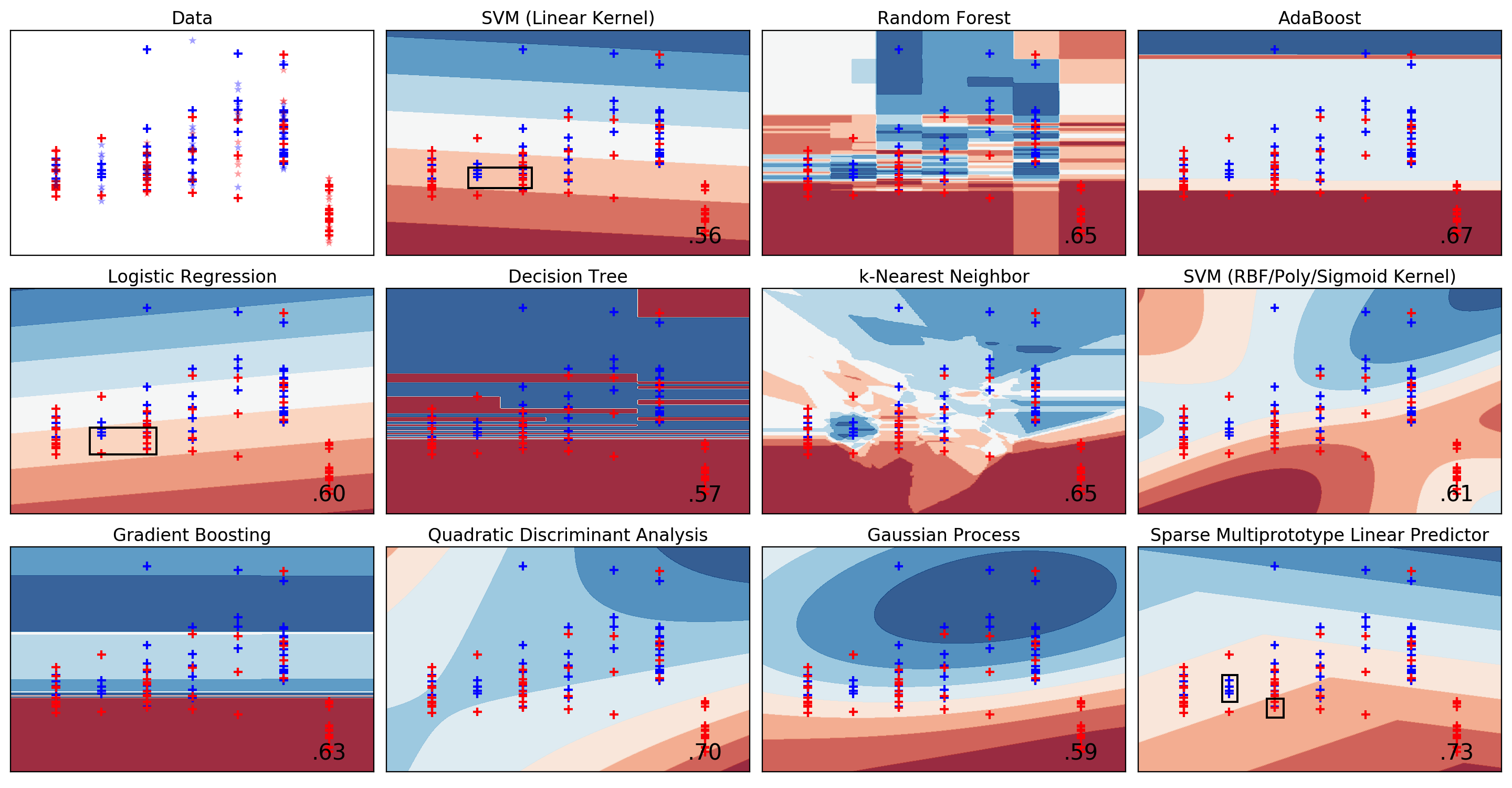
Figure 1: Decision surfaces of different classifier types on the two-dimensional chscase funds toy dataset. Test classification accuracy is shown on the bottom right of each plot.

We now derive a saddle-point formulation of the mixed-integer nonlinear optimization problem (9). We can then derive a convex-concave relaxation that can be solved efficiently by the Mirror-Prox algorithm.

3 Saddle-Point Relaxation

We show that problem in (9) is equivalent to the following minimax saddle-point problem:

$$\min_{\begin{subarray}{c}{W\in\mathbb{R}^{p\times n}}\\ \epsilon\in\{0,1\}^{p\times n}\\ ||\epsilon||_{1,\infty}\leq k\end{subarray}}~{}\max_{\begin{subarray}{c}S=[s_{1}\cdots s_{m}]\\ s_{i}\in\mathcal{S}_{i},~{}i\in[m]\end{subarray}}~{}\Phi(W,\epsilon,S),$$ (10)

where $S\in\mathbb{R}^{p\times m}$, each of its column $s_{i}$ belongs to a set $\mathcal{S}_{i}\subset\mathbb{R}^{p}$ (which are given in Proposition 1), and

$$\Phi(W,\epsilon,S)\!=\!\frac{1}{m}\!\!\sum_{i\in[m]}\!\Bigl{(}y_{i}s_{i}^{T}(W\odot\epsilon)x_{i}-u^{\star}(s_{i})\!\Bigr{)}+\dfrac{\lambda}{2}||W||_{F}^{2}.$$

Here $u^{\star}$ is the convex conjugate of $u$ defined in (6):

$$u^{\star}(s_{i})=\sup_{t\in\mathbb{R}^{p}}\bigl{\{}s_{i}^{T}t-u(t)\bigr{\}}$$ (11)

$$=\begin{cases}\displaystyle\sum_{j=1}^{p}(-s_{i,j})\log(-s_{i,j})+(1\!+\!{\bf 1}^{T}s_{i})\log(1\!+\!{\bf 1}^{T}s_{i}),\\ \qquad\quad\mbox{if }s_{i,j}\leq 0~{}\forall j\in[p]$ and ${\bf 1}^{T}s_{i}\geq-1;\\ \infty,\hskip 11.38092pt\mbox{ otherwise }.\end{cases}$$

The equivalence between (9) and (10) is a direct consequence of the following proposition.

Proposition 1.

Let $\ell(z)=\log(1+\exp(-z))$ where $z\in\mathbb{R}$ and $u(t)=\log\bigl{(}1+\sum_{j\in[p]}\exp(-t_{j})\bigr{)}$ where $t\in\mathbb{R}^{p}$. Then for $i\in I_{+}$, we have

$$\ell\bigl{(}(W\odot\epsilon)_{j(i)}x_{i}\bigr{)} =\max_{s_{i}\in\mathcal{S}_{i}}\left(y_{i}s_{i}^{T}(W\odot\epsilon)x_{i}-u^{\star}(s_{i})\right),$$

where $y_{i}=+1$ and

$$\mathcal{S}_{i}=\Bigl{\{}s_{i}\in\mathbb{R}^{p}:s_{i,j(i)}\!\in\![-1,0],~{}s_{i,j}\!=\!0~{}\forall j\neq\!j(i)\Bigr{\}}.$$

For $i\in I_{-}$, we have

$$u\bigl{(}-(W\odot\epsilon)x_{i}\bigr{)} =\max_{s_{i}\in\mathcal{S}_{i}}\left(y_{i}s_{i}^{T}(W\odot\epsilon)x_{i}-u^{\star}(s_{i})\right),$$

where $y_{i}=-1$ and

$$\mathcal{S}_{i}=\Bigl{\{}s_{i}\in\mathbb{R}^{p}:{\bf 1}^{T}s\geq-1,~{}s_{i,j}\leq 0~{}\forall j\in[p]\Bigr{\}}.$$

We can further eliminate the variable $W$ in (10), which is facilitated by the following result.

Proposition 2.

For any given $\epsilon\in\{0,1\}^{p\times n}$ and $S\in\mathcal{S}_{1}\times\cdots\times\mathcal{S}_{m}$, the solution to

$$\min_{W\in\mathbb{R}^{p\times n}}\Phi(W,\epsilon,S)$$

is unique and given by

$$W(\epsilon,S)=-\frac{1}{m\lambda}\sum_{i\in[m]}y_{i}\bigl{(}s_{i}x_{i}^{T}\bigr{)}\odot\epsilon.$$ (12)

Now we substitute $W(\epsilon,S)$ into (10) to obtain

$$\min_{\begin{subarray}{c}\epsilon\in\{0,1\}^{p\times n}\\ \|\epsilon\|_{1,\infty}\leq k\end{subarray}}~{}\max_{\begin{subarray}{c}S=[s_{1}\cdots s_{m}]\\ s_{i}\in\mathcal{S}_{i},~{}i\in[m]\end{subarray}}~{}\phi(\epsilon,S),$$ (13)

where

$$\phi(\epsilon,S)=-\frac{1}{m\lambda}\biggl{\|}\sum_{i\in[m]}y_{i}\bigl{(}s_{i}x_{i}^{T}\bigr{)}\odot\epsilon\biggr{\|}_{F}^{2}-\sum_{i\in[m]}u^{\star}(s_{i}).$$

The above expression of $\phi(\epsilon,S)$ is concave in $S$ (which is to be maximized), but not convex in $\epsilon$ (which is to be minimized). However, because $\epsilon\in\{0,1\}^{p\times n}$,

$$\biggl{\|}\sum_{i\in[m]}y_{i}\bigl{(}s_{i}x_{i}^{T}\bigr{)}\odot\epsilon\biggr{\|}_{F}^{2}$$

$$= \sum_{i\in[m]}y_{i}s_{i}^{T}\biggl{(}\sum_{i\in[m]}y_{i}\bigl{(}s_{i}x_{i}^{T}\bigr{)}\odot\epsilon\odot\epsilon\biggr{)}x_{i}$$

$$= \sum_{i\in[m]}y_{i}s_{i}^{T}\biggl{(}\sum_{i\in[m]}y_{i}\bigl{(}s_{i}x_{i}^{T}\bigr{)}\odot\epsilon\biggr{)}x_{i},$$

where we used $\epsilon\odot\epsilon=\epsilon$. Therefore we have

$$\phi(\epsilon,S)= -\frac{1}{m\lambda}\sum_{i\in[m]}y_{i}s_{i}^{T}\biggl{(}\sum_{i\in[m]}y_{i}\bigl{(}s_{i}x_{i}^{T}\bigr{)}\odot\epsilon\biggr{)}x_{i}$$

$$-\sum_{i\in[m]}u^{\star}(s_{i}),$$ (14)

which is concave in $S$ and linear (thus convex) in $\epsilon$.

Finally, we relax the integrality constraint on $\epsilon$ to its convex hull, i.e., $\epsilon\in[0,1]^{p\times n}$, and consider

$$\min_{\begin{subarray}{c}\epsilon\in[0,1]^{p\times n}\\ \|\epsilon\|_{1,\infty}\leq k\end{subarray}}~{}\max_{\begin{subarray}{c}S=[s_{1}\cdots s_{m}]\\ s_{i}\in\mathcal{S}_{i},~{}i\in[m]\end{subarray}}~{}\phi(\epsilon,S),$$ (15)

where $\phi(\epsilon,S)$ is given in (14). This is a convex-concave saddle-point problem, which can be solved efficiently (in polynomial time) by the Mirror-Prox algorithm [20, 15].

After finding a solution $(\epsilon,S)$ of (15), we can round the entries of $\epsilon$ to $\{0,1\}$, while respecting the constraint $\|\epsilon\|_{1,\infty}\leq k$ (for example, rounding the largest $k$ entries of each row to $1$ and the rest entries to $0$). Then we can recover the prototypes using the formula (12).

Table 1: Comparison of test accuracy of the different classification algorithms on low dimensional ($n<20$) OpenML datasets. ‘-’ indicates that GP failed to yield a solution in all the runs. $K$, in SMaLL, was set to $n$ for these data.

	LSVM	RF	AB	LR	DT	kNN	RSVM	GB	QDA	GP	SMaLL
bankruptcy	.84$\pm$.07	.83$\pm$.08	.82$\pm$.05	.90$\pm$.05	.80$\pm$.05	.78$\pm$.07	.89$\pm$.06	.81$\pm$.05	.78$\pm$.15	.90$\pm$.05	.92$\pm$.06
vineyard	.79$\pm$.10	.72$\pm$.06	.68$\pm$.04	.82$\pm$.08	.69$\pm$.13	.70$\pm$.11	.82$\pm$.07	.68$\pm$.09	.75$\pm$.07	.71$\pm$.12	.83$\pm$.07
pwLinear	.83$\pm$.02	.85$\pm$.03	.83$\pm$.04	.85$\pm$.02	.80$\pm$.05	.78$\pm$.04	.85$\pm$.03	.85$\pm$.03	.87$\pm$.01	-	.85$\pm$.02
sleuth1714	.82$\pm$.03	.82$\pm$.04	.81$\pm$.14	.83$\pm$.04	.83$\pm$.06	.82$\pm$.04	.76$\pm$.03	.82$\pm$.06	.63$\pm$.13	.80$\pm$.03	.83$\pm$.05
sleuth1605	.66$\pm$.09	.70$\pm$.07	.64$\pm$.08	.70$\pm$.07	.63$\pm$.09	.66$\pm$.05	.65$\pm$.09	.65$\pm$.09	.62$\pm$.05	.72$\pm$.07	.72$\pm$.05
sleuth1201	.94$\pm$.05	.94$\pm$.03	.92$\pm$.05	.93$\pm$.03	.91$\pm$.05	.90$\pm$.04	.89$\pm$.09	.88$\pm$.06	.89$\pm$.07	.91$\pm$.08	.94$\pm$.05
rabe266	.93$\pm$.04	.90$\pm$.03	.91$\pm$.04	.92$\pm$.04	.91$\pm$.03	.92$\pm$.03	.93$\pm$.04	.90$\pm$.04	.94$\pm$.03	.95$\pm$.04	.94$\pm$.02
rabe148	.95$\pm$.04	.93$\pm$.04	.91$\pm$.08	.95$\pm$.04	.89$\pm$.07	.92$\pm$.05	.91$\pm$.06	.91$\pm$.08	.92$\pm$.09	.95$\pm$.02	.96$\pm$.04
vis_env	.66$\pm$.04	.68$\pm$.05	.66$\pm$.03	.65$\pm$.08	.62$\pm$.04	.57$\pm$.03	.69$\pm$.06	.64$\pm$.03	.62$\pm$.07	.65$\pm$.09	.69$\pm$.03
hutsof99	.74$\pm$.07	.66$\pm$.04	.64$\pm$.09	.73$\pm$.07	.60$\pm$.10	.66$\pm$.11	.66$\pm$.14	.67$\pm$.05	.59$\pm$.07	.70$\pm$.05	.75$\pm$.04
human_dev	.88$\pm$.03	.85$\pm$.04	.85$\pm$.03	.89$\pm$.04	.85$\pm$.03	.87$\pm$.03	.88$\pm$.03	.86$\pm$.03	.88$\pm$.03	.88$\pm$.02	.89$\pm$.04
fri_c0_100_10	.77$\pm$.04	.74$\pm$.03	.76$\pm$.03	.77$\pm$.03	.64$\pm$.07	.71$\pm$.05	.79$\pm$.03	.71$\pm$.05	.74$\pm$.03	.78$\pm$.01	.77$\pm$.06
elusage	.90$\pm$.05	.84$\pm$.06	.84$\pm$.06	.89$\pm$.04	.84$\pm$.06	.87$\pm$.05	.89$\pm$.04	.84$\pm$.06	.90$\pm$.04	.89$\pm$.04	.92$\pm$.04
diggle_table	.65$\pm$.14	.61$\pm$.07	.57$\pm$.08	.65$\pm$.11	.60$\pm$.09	.58$\pm$.07	.57$\pm$.13	.57$\pm$.06	.62$\pm$.07	.60$\pm$.13	.68$\pm$.07
baskball	.70$\pm$.02	.68$\pm$.04	.68$\pm$.02	.71$\pm$.03	.71$\pm$.03	.63$\pm$.02	.66$\pm$.05	.69$\pm$.04	.69$\pm$.04	.68$\pm$.02	.72$\pm$.06
michiganacc	.72$\pm$.06	.67$\pm$.06	.71$\pm$.05	.71$\pm$.04	.67$\pm$.06	.66$\pm$.07	.71$\pm$.05	.69$\pm$.04	.72$\pm$.04	.71$\pm$.05	.73$\pm$.05
election2000	.92$\pm$.04	.90$\pm$.04	.91$\pm$.03	.92$\pm$.02	.91$\pm$.03	.92$\pm$.01	.90$\pm$.07	.92$\pm$.02	.72$\pm$.06	.92$\pm$.03	.94$\pm$.02

3.1 The Mirror-Prox Algorithm

Algorithm 1 Mirror-Prox algorithm for solving (15)

1:Initialize $\epsilon^{(0)}$ and $\epsilon^{(0)}$

2:for $t=0,1,\ldots,T$ do

3:     Gradient step:

4:     $\hat{\epsilon}^{(t)}=\mathrm{Proj}_{\mathcal{E}}\bigl{(}\epsilon^{(t)}-\alpha_{t}\nabla_{\epsilon}\phi(\epsilon^{(t)},S^{(t)})\bigr{)}$

5:     $\hat{s}_{i}^{(t)}\!=\mathrm{Proj}_{\mathcal{S}_{i}}\bigl{(}s_{i}^{(t)}\!+\beta_{t}\nabla_{s_{i}}\phi(\epsilon^{(t)},S^{(t)})\bigr{)},~{}i\in[m]$

6:     Extra-gradient step:

7:     $\epsilon^{(t+1)}=\mathrm{Proj}_{\mathcal{E}}\bigl{(}\epsilon^{(t)}-\alpha_{t}\nabla_{\epsilon}\phi(\hat{\epsilon}^{(t)},\hat{S}^{(t)})\bigr{)}$

8:     $s_{i}^{(t+1)}\!=\mathrm{Proj}_{\mathcal{S}_{i}}\!\bigl{(}s_{i}^{(t)}\!+\beta_{t}\nabla_{s_{i}}\phi(\hat{\epsilon}^{(t)},\hat{S}^{(t)})\bigr{)},~{}i\!\in\![m]$

9:end for

10:$\hat{\epsilon}=\sum_{t=1}^{T}\alpha_{t}\,\hat{\epsilon}^{(t)}\big{/}\sum_{t=1}^{T}\alpha_{t}$

11:$\hat{S}=\sum_{t=1}^{T}\beta_{t}\,\hat{S}^{(t)}\big{/}\sum_{t=1}^{T}\beta_{t}$

12:Round $\hat{\epsilon}$ to $\{0,1\}^{p\times n}$

13:$\hat{W}=-\frac{1}{m\lambda}\sum_{i\in[m]}y_{i}(\hat{s}_{i}x_{i}^{T})\odot\hat{\epsilon}$

Algorithm 1 is a customized Mirror-Prox algorithm for solving the convex-concave saddle-point problem (15), which enjoys a $O(1/t)$ convergence rate [20, 15].

The partial gradients of $\phi(\epsilon,S)$ are given as

$$\nabla_{\epsilon}\phi(\epsilon,S) =-\frac{1}{m\lambda}\biggl{(}\sum_{i\in[m]}y_{i}\bigl{(}s_{i}x_{i}^{T}\bigr{)}\!\biggr{)}\odot\biggl{(}\sum_{i\in[m]}y_{i}\bigl{(}s_{i}x_{i}^{T}\bigr{)}\!\biggr{)},$$

$$\nabla_{s_{i}}\phi(\epsilon,S) =-\frac{1}{m\lambda}y_{i}\biggl{(}\sum_{i\in[m]}y_{i}\bigl{(}s_{i}x_{i}^{T}\bigr{)}\odot\epsilon\biggr{)}x_{i},~{}~{}i\in[m].$$

There are two projection operators in Algorithm 1. The first one is to project some $\epsilon\in\mathbb{R}^{p\times n}$ onto the convex set

$$\mathcal{E}\triangleq\left\{\epsilon\in\mathbb{R}^{p\times n}:\epsilon\in[0,1]^{p\times n},~{}\|\epsilon\|_{1,\infty}\leq k\right\},$$

which can be done efficiently by Algorithm 2. Essentially, we perform $p$ independent projections, each for one row of $\epsilon$ using a bi-section type of algorithm [4, 21, 9]. We prove the following result in the appendix.

Proposition 3.

Algorithm 2 computes, up to a specified tolerance $tol$, the projection of any $\epsilon\in\mathbb{R}^{p\times n}$ onto $\mathcal{E}$ in $\mathcal{O}\left(\log_{2}(1/tol)\right)$ time.

There are two case for the projection of $s_{i}\in\mathbb{R}^{p}$ onto the set $S_{i}$. For $i\in I_{+}$, we only need to project $s_{i,j(i)}$ onto the interval $[-1,0]$ and set $s_{i,j}=0$ for all $j\neq j(i)$. For $i\in I_{-}$, the projection algorithm is similar to Algorithm 2, and we omit the details here.

For the step sizes $\alpha_{t}$ and $\beta_{t}$, they can be set according to the guidelines described in [20, 15], which depends on the smoothness properties of the function $\phi(\epsilon,S)$. In practice, we follow the adaptive tuning procedure developed in [14].

Algorithm 2 $(\mathrm{Proj}_{\mathcal{E}})$ Projection of a vector onto
          $\mathcal{E}_{j}\triangleq\{\epsilon_{j}\in\mathbb{R}^{n}:\epsilon_{ji}\in[0,1],~{}\|\epsilon_{j}\|_{1}\leq k\}$.
Given input $\epsilon_{j}\in\mathbb{R}^{n}$ and a small tolerance $tol$.

1:$\mbox{Clip}~{}\epsilon_{j}~{}\mbox{to}[0,1]^{n}:~{}\hat{\epsilon}_{j,i}=\begin{cases}0&\mbox{ if }\epsilon_{j,i}\leq 0\\ 1&\mbox{ if }\epsilon_{j,i}\geq 1\\ \epsilon_{j,i}&\mbox{otherwise}\end{cases},~{}i\in[n]\$

2:Return $\hat{\epsilon}_{j}$ if ${\bf 1}^{T}\hat{\epsilon}_{j}\leq k$

3:      Do binary search until $tol$-solution found

4:Set $low=\left({\bf 1}^{T}\epsilon_{j}-k\right)/n$

5:Set $high=\max_{i\in[n]}\epsilon_{j,i}-k/n$

6:while $low\leq high$ do

7:     Set $\lambda=(low+high)/2$

8:     Compute $\hat{\epsilon_{j}}:\forall i\in[n],\hat{\epsilon}_{j,i}=\epsilon_{j,i}-\lambda$

9:     Clip $\hat{\epsilon}_{j}$ to $[0,1]^{n}$

10:     if $|{\bf 1}^{T}\hat{\epsilon}_{j}-k|<tol$ then

11:         return $\hat{\epsilon}_{j}$

12:     else if ${\bf 1}^{T}\hat{\epsilon}_{j}>k$ then

13:         Set $low=(low+high)/2$

14:     else

15:         Set $high=(low+high)/2$

16:     end if

17:end while

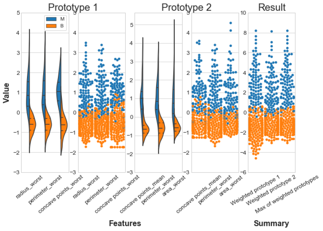
Figure 2: SMaLL applied to the Breast Cancer dataset with $k=3$ and $p=2$. The blue and the orange dots represent the test instances from the two classes. The plots show the kernel density estimates and the actual values of the non-zero features in each prototype, as well at the final predictor result.

4 Experiments

We demonstrate the merits of our approach with a set of experiments. First, we attempt to give some intuition on how the class of sparse multiprototype linear predictors differs from other popular model classes. Figure 1 is a visualization of the decision surface of different types of classifiers on the 2-dimensional chscase funds toy dataset, obtained from OpenML. The two classes are shown in red and blue, with training data in solid shade and test data in translucent shade. The color of each band indicates the gradation in the confidence of prediction - each classifier is more confident in the darker regions and less confident in the lighter regions. The $2$-prototype linear predictor attains the best test accuracy on this toy problem ($0.73$). Note that some of the examples are highlighted by a black rectangle - the linear classifiers (logistic regression and linear SVM) could not distinguish between these examples, whereas the $2$-prototype linear predictor was able to distinguish and assign them to different bands.

4.1 Low-dimensional Datasets Without Sparsity

Next, we compare the accuracy of SMaLL with $k=n$ (no sparsity) to the accuracy of other standard classification algorithms, on various low-dimensional ($n\leq 20$) binary classification datasets from OpenML. The methods that we compare against are: linear SVM (LSVM), SVM with non-linear kernels such as radial basis function, polynomial, and sigmoid (RSVM), Logistic Regression (LR), Decision Trees (DT), Random Forest (RF), $k$-Nearest Neighbor (kNN), Gaussian Process (GP), Gradient Boosting (GB), AdaBoost (AB), and Quadratic Discriminant Analysis (QDA). All the datasets were normalized so that each feature has zero mean and unit variance. Since the datasets do not specify separate train, validation, and test sets, we measure test accuracy by averaging over five random train-test splits. We pre-clustered the positive examples into $p=2$ clusters, and initialized the prototypes with the cluster centers.

We trained parameters by $5$-fold cross-validation. The coefficient of the error term $C$ in LSVM and $\ell_{2}$-regularized LR was selected from $\{0.1,1,10,100\}$. In the case of RSVM, we also added $0.01$ to the search set for $C$, and chose the best kernel between a radial basis function (RBF), polynomials of degree 2 and 3, and sigmoid. For the ensemble methods (RF, AB, GB), the number of base predictors was selected from the set $\{10,20,50\}$. The maximum number of features for RF estimators was optimized over the square root and the log selection criteria. We also found best validation parameters for DT (gini or entropy for attribute selection), kNN (1, 3, 5 or 7 neighbors), and GP (RBF kernel scaled with scaled by a coefficient in the set $\{0.1,1.0,5\}$ and dot product kernel with inhomogeneity parameter $\sigma$ set to 1). Finally, for our algorithm SMaLL, we fixed $\lambda=0.1$ and $\alpha_{t}=0.01$, and we searched over $\beta_{t}=\beta\in\{0.01,0.001\}$.

Table 1 shows the test accuracy for the different algorithms on different datasets. As seen from the table, SMaLL with $k=n$ generally performed very well on most of these datasets. This substantiates the practicality of SMaLL in the low dimensional regime.

4.2 Higher-Dimensional Datasets with Sparsity

On higher-dimensional data, feature selection becomes critical. To substantiate our claim that our technique produces an interpretable model, we ran SMaLL on the Breast Cancer dataset with $k=3$ and $p=2$ (two prototypes, three non-zero elements in each). Figure 2 shows the kernel density estimate plots and the actual values of the non-zero features in each prototype, as well at the final predictor result. Note that the feature perimeter_worst appears in both prototypes. As the rightmost plot shows, the predictor output provides a good separation of the test data, and SMaLL registered a test accuracy of over $94\%$. It is straightforward to understand how the resulting classifier reaches its decisions: which features it relies on and how those features interact.

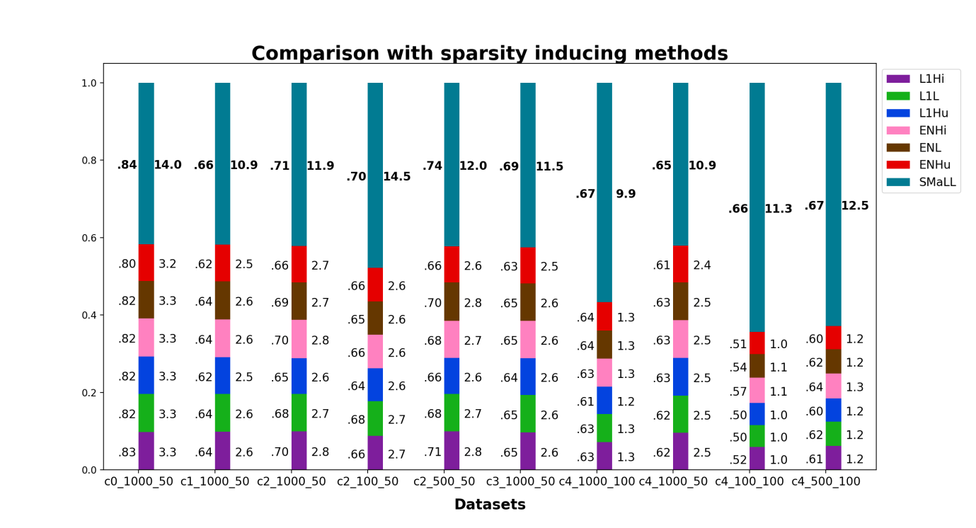
Figure 3: Comparison on high dimensional ($n>=50$) OpenML datasets. Each stacked bar shows two numbers: average test accuracy on the left, and the ratio of average test accuracy in % to the number of selected features on the right.

Next, we compare SMaLL with six other methods, which induce sparsity by minimizing an $\ell_{1}$-regularized loss function. These methods minimize one of three empirical loss functions (hinge loss, log loss, and the binary-classification Huber loss), regularized by either an $\ell_{1}$ or an elastic net penalty (i.e. $\ell_{1}$ and $\ell_{2}$). We refer to these as L1Hi ($\ell_{1}$, hinge), L1L ($\ell_{1}$, log), L1Hu ($\ell_{1}$, Huber), EnHi (elastic net, hinge), ENL (elastic net, log) and ENHu (elastic net, huber).

Note that while we can explicitly control the amount of sparsity in SMaLL, the methods that use $\ell_{1}$ or Elastic Net regularization do not have this flexibility. Therefore, in order to get the different baselines on the same footing, we devised the following empirical methodology. We trained each baseline and selected the $n/2$ features with the largest absolute values. Then, we retrained the classifier using only the selected features, using the same loss (hinge, loss, or log) and an $\ell_{2}$ regularization. Our procedure ensured that each baseline benefited, in effect, from an elastic net-like regularization while having the most important features at its disposal. For the SMaLL classifier, we fixed $k=3$ and $p=2$. As before, when the original dataset did not specify a train-test split, our results are averaged over five random splits. The parameters for each method were tuned using a 5-fold grid search cross-validation procedure. We fixed $\lambda=0.1$ and $\eta=1e-4$, and performed a joint search over $\alpha_{t}\in\{0.1,1e-2,1e-3\}$ and $\beta_{t}\in\{1e-3,1e-4\}$. For all the baselines, we optimized the cross validation error over the $\ell_{1}$ regularization coefficients in the set $\{1e-1,1e-2,1e-3,1e-4\}$. Moreover, in case of elastic net, the ratio of the $\ell_{1}$ coefficient to the $\ell_{2}$ coefficient was set to 1.

Figure 3 provides empirical evidence that SMaLL yields extremely sparse yet more accurate prototypes than the baselines on several high dimensional OpenML datasets. The first number in each dataset name indicates the number of examples, and the second the dimensionality. In SMaLL, since some features might be selected in more than one prototype, we included the multiplicity while computing the total feature count. Each bar in the plot is scaled to unit length, with each method getting a share proportional to its normalized accuracy on the dataset. The normalized accuracy indicates the effective information conveyed per selected feature. We see that SMaLL outperforms other methods in both accuracy as well as the normalized performance, the latter by an order of magnitude. This shows the promise of convex relaxations of SMaLL toward achieving succinct yet accurate weight representation in the high dimensional regime. In fact, as Fig. 3 shows, the savings in terms of sparsity could be truly remarkable. This observation is further reinforced in Fig. 4. We observe that SMaLL registers a normalized value over 14, which is significantly higher than all the other methods, without incurring a significant dip in test accuracy compared to the most accurate method (GB).

Appendix A Supplementary Material

Proof of Proposition 1

Proof.

By definition, the Fenchel conjugate

$$u^{*}(s)=\sup_{t\in\mathbb{R}^{p}}\left(\sum_{k=1}^{p}s_{k}t_{k}-\log\left(1+\sum_{k=1}^{p}\exp(-t_{k})\right)\right).$$

Equating the partial derivative with respect to each $t_{k}$ to 0, we get

$$s_{k}~{}=~{}-\dfrac{\exp(-t_{k}^{*})}{1+\sum_{c=1}^{p}\exp(-t_{c}^{\ast})}~{}~{},$$ (16)

or equivalently,

$$t_{k}^{*}=-\log\left(-s_{k}\left(1+\sum_{c=1}^{p}\exp(-t_{c}^{*})\right)\right)~{}~{}.$$

We note from (16) that

$$\dfrac{1}{1+\sum_{c=1}^{p}\exp(-t_{c}^{*})}=1+s^{\top}{\bf 1}~{}~{}.$$

Using the convention $0\log 0=0$, the form of the conjugate function in (11) can be obtained by plugging $t^{*}=(t_{1}^{*},\ldots,t_{r}^{*})$ into $u^{*}(s)$ and performing some simple algebraic manipulations.

Proposition 1 follows directly from the form of $u^{*}$, especially the constraint set $\mathcal{S}_{i}$ for $i\in I_{-}$. For $i\in I_{+}$, we notice that the conjugate of $\ell(z)=\log(1+\exp(-z))$ is

$$\ell^{*}(\beta)=(-\beta)\log(-\beta)+(1+\beta)\log(1+\beta),\quad\beta\in[-1,0].$$

Then we can let the $j(i)$th entry of $s_{i}\in\mathbb{R}^{p}$ be $\beta\in[-1,0]$ and all other entries be zero. Then we can express $\ell^{*}$ through $u^{*}$ as shown in the proposition. ∎

Proof of Proposition 2

Proof.

Recall that

$$\Phi(W,\epsilon,S)\!=\!\frac{1}{m}\!\!\sum_{i\in[m]}\!\Bigl{(}y_{i}s_{i}^{T}(W\odot\epsilon)x_{i}-u^{*}(s_{i})\!\Bigr{)}+\dfrac{\lambda}{2}||W||_{F}^{2}.$$

Then

$$\nabla_{W}\Phi(W,\epsilon,S)\!=\!\frac{1}{m}\!\!\sum_{i\in[m]}y_{i}\bigl{(}s_{i}x_{i}^{T}\bigr{)}\odot\epsilon+\lambda W~{}~{}.$$

The proof is complete by setting $\nabla_{W}\Phi(W,\epsilon,S)=0$, and solving for $W$. ∎

Proof of Proposition 3

Proof.

In order to project $a\in\mathbb{R}^{n}$ onto

$$\mathcal{E}_{j}\triangleq\{\epsilon_{j}\in\mathbb{R}^{n}:\epsilon_{ji}\in[0,1],~{}\|\epsilon_{j}\|_{1}\leq k\},$$

we need to solve the following problem:

$$\min_{x\in\mathbb{R}^{n}} \dfrac{1}{2}||x-a||^{2}$$

s.t. $$\sum_{i=1}^{d}x_{i}\leq k$$

$$\forall i\in[n]: 0\leq x_{i}\leq 1~{}~{}.$$

Our approach is to form a Lagrangian and then invoke the KKT conditions. Introducing Lagrangian parameters $\lambda\in\mathbb{R}_{+}$ and $u,v\in\mathbb{R}_{+}^{d}$, we get the Lagrangian $L(x,\lambda,u,v)$

$$= \dfrac{1}{2}||x-a||^{2}+\lambda\left(\sum_{i=1}^{n}x_{i}-k\right)-\sum_{i=1}^{n}u_{i}x_{i}$$

$$\qquad\qquad+ \sum_{i=1}^{n}v_{i}(x_{i}-1)$$

$$= \dfrac{1}{2}||x-a||^{2}+\sum_{i=1}^{n}x_{i}(\lambda-u_{i}+v_{i})$$

$$\qquad\qquad- \lambda k-\sum_{i=1}^{n}v_{i}~{}~{}.$$

Therefore,

$$\nabla_{x^{*}}L=0\implies x^{*}=a-(\lambda\mathbf{1}-u+v)~{}~{}.$$ (17)

We note that $g(\lambda,u,v)\triangleq L(x^{*},\lambda,u,v)$

$$=~{}-\dfrac{1}{2}||\lambda\mathbf{1}-u+v||^{2}+a^{\top}(\lambda\mathbf{1}-u+v)-\lambda K-\mathbf{1}^{\top}v.$$

Using the notation $b\succeq t$ to mean that each coordinate of vector $b$ is at least $t$, our dual is

$$\max_{\lambda\geq 0,u\succeq 0,v\succeq 0}g(\lambda,u,v)~{}~{}.$$ (18)

We now list all the KKT conditions:

$$\forall i\in[n]:\qquad x_{i}>0 \implies u_{i}=0$$

$$\forall i\in[n]:\qquad x_{i}<1 \implies v_{i}=0$$

$$\forall i\in[n]:\qquad u_{i}>0 \implies x_{i}=0$$

$$\forall i\in[n]:\qquad v_{i}>0 \implies x_{i}=1~{}~{}~{}~{}~{}~{}~{}.$$

$$\forall i\in[n]:\qquad u_{i}v_{i} = 0$$

$$\sum_{i=1}^{n}x_{i}<k \implies \lambda=0$$

$$\lambda>0 \implies \sum_{i=1}^{n}x_{i}=k$$

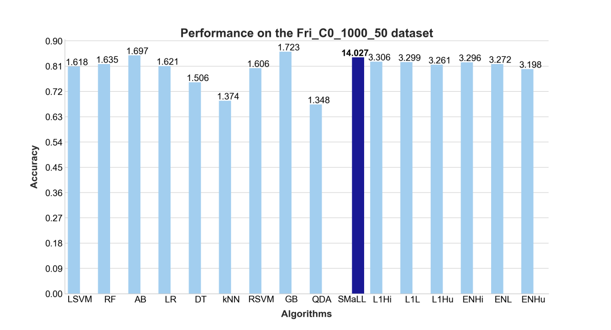
Figure 4: The big picture. The plot depicts the performance of SMaLL to both the standard classification algorithms and the sparsity inducing baselines on the fri_c0_1000_50 dataset. The dataset consists of 1000 examples in 50 dimensions. The number atop each bar is the ratio of average test accuracy in percentage to the average number of selected features.

We consider the two cases, (a) $\sum_{i=1}^{n}x^{*}_{i}<k$, and (b) $\sum_{i=1}^{n}x^{*}_{i}=k$ separately.

First consider $\sum_{i=1}^{n}x^{*}_{i}<k$. Then, by KKT conditions, we have the corresponding $\lambda=0$. Consider all the sub-cases. Using (17), we get

1. $x^{*}_{i}=0\implies a_{i}=\lambda-u_{i}+v_{i}=-u_{i}\leq 0$ (since $x^{*}_{i}<1$, therefore, by KKT conditions, $v_{i}=0$).

2. $x^{*}_{i}=1\implies a_{i}=1+\lambda-u_{i}+v_{i}=1+v_{i}\geq 1$ (since $x^{*}_{i}>0$, therefore, $u_{i}=0$ by KKT conditions).

3. $0<x^{*}_{i}<1\implies a_{i}=x^{*}_{i}+\lambda-u_{i}+v_{i}=x^{*}_{i}$.

Now consider $\sum_{i=1}^{n}x^{*}_{i}=k$. Then, we have $\lambda\geq 0$. Again, we look at the various sub-cases.

1. $x^{*}_{i}=0\implies a_{i}=\lambda-u_{i}+v_{i}=\lambda-u_{i}\implies u_{i}=-(a_{i}-\lambda)$. Here, $u_{i}$ denotes the amount of clipping done when $a_{i}$ is negative.

2. $x^{*}_{i}=1\implies a_{i}=1+\lambda-u_{i}+v_{i}=1+\lambda+v_{i}\implies v_{i}=-(1+\lambda-a_{i})$. Here, $v_{i}$ denotes the amount of clipping done when $a_{i}>1$. Also, note that $a_{i}\geq 1$ in this case.

3. $0<x^{*}_{i}<1\implies a_{i}=x^{*}_{i}+\lambda-u_{i}+v_{i}=x^{*}_{i}+\lambda\implies x^{*}_{i}=a_{i}-\lambda$. In order to determine the value of $\lambda$, we note that since $\sum_{i=1}^{n}x^{*}_{i}=k$, therefore,

   $$\sum_{i=1}^{n}(a_{i}-\lambda)=k\implies\sum_{i=1}^{n}a_{i}-n\lambda=k$$

   $$\implies\lambda=\dfrac{1}{n}\sum_{i=1}^{n}a_{i}-\dfrac{k}{n}\leq\max_{i}a_{i}-\dfrac{k}{n}~{}~{}.$$

Algorithm 2 implements these different sub-cases and thus accomplishes the desired projection. The algorithm is a bisection method, and thus converges linearly to a solution within the specified tolerance $tol$. ∎

References

• Blum & Rudich, [1995] Blum, A., & Rudich, S. 1995. Fast learning of k-term DNF formulas with queries. Journal of Computer and System Sciences, 51(3), 367–373.
• Blum et al. , [1994] Blum, A., Furst, M., Jackson, J., Kearns, M., Mansour, Y., & Rudich, S. 1994. Weakly learning DNF and characterizing statistical query learning using Fourier analysis. Pages 253–262 of: Proceedings of the Twenty-sixth Annual ACM Symposium on Theory of Computing (STOC).
• Boyd & Vandenberghe, [2004] Boyd, S., & Vandenberghe, L. 2004. Convex Optimization. Cambridge University Press.
• Brucker, [1984] Brucker, P. 1984. An $O(n)$ algorithm for quadratic Knapsack problems. Operations Research Letters, 3(3), 163–166.
• Bshouty, [1996] Bshouty, N. H. 1996. A subexponential exact learning algorithm for DNF using equivalence queries. Information Processing Letters, 59(1), 37–39.
• Bshouty et al. , [1999] Bshouty, N. H., Jackson, J. C., & Tamon, C. 1999. More efficient PAC-learning of DNF with membership queries under the uniform distribution. Pages 286–295 of: Proceedings of the Twelfth Annual Conference on Computational Learning Theory (COLT).
• Bshouty et al. , [2005] Bshouty, N. H., Mossel, E., O’Donnell, R., & Servedio, R. A. 2005. Learning DNF from random walks. Journal of Computer and System Sciences, 71(3), 250–265.
• Cord, [2001] Cord, O. 2001. Genetic fuzzy systems: evolutionary tuning and learning of fuzzy knowledge bases. Vol. 19. World Scientific.
• Duchi et al. , [2008] Duchi, J., Shalev-Shwartz, S., Singer, Y., & Chandra, T. 2008. Efficient projection onto the $\ell_{1}$-ball for learning in high dimensions. Pages 272–279 of: Proceedings of the 25th International Conference on Machine Learning.
• Feldman, [2012] Feldman, V. 2012. Learning DNF expressions from fourier spectrum. Pages 17.1–17.19 of: Conference on Learning Theory (COLT).
• Gupta et al. , [2017] Gupta, C., Suggala, A. S., Goyal, A., Simhadri, H. V., Paranjape, B., Kumar, A., Goyal, S., Udupa, R., Varma, M., & Jain, P. 2017. ProtoNN: Compressed and Accurate kNN for Resource-scarce Devices. Pages 1331–1340 of: International Conference on Machine Learning.
• Hauser et al. , [2010] Hauser, J. R., Toubia, O., Evgeniou, T., Befurt, R., & Dzyabura, D. 2010. Disjunctions of conjunctions, cognitive simplicity, and consideration sets. Journal of Marketing Research, 47(3), 485–496.
• Jackson, [1997] Jackson, J. C. 1997. An efficient membership-query algorithm for learning DNF with respect to the uniform distribution. Journal of Computer and System Sciences, 55(3), 414–440.
• Jalali et al. , [2017] Jalali, A., Fazel, M., & Xiao, L. 2017. Variational Gram Functions: Convex Analysis and Optimization. SIAM Journal on Optimization, 27(4), 2634–2661.
• Juditsky & Nemirovski, [2011] Juditsky, A., & Nemirovski, A. 2011. First-order methods for nonsmooth convex large-scale optimization, II: Utilizing problems’s structure. Chap. 6, pages 149–184 of: Sra, S., Nowozin, S., & Wright, S. J. (eds), Optimization for Machine Learning. Cambridge, MA.: The MIT Press.
• Khot & Saket, [2008] Khot, S., & Saket, R. 2008. Hardness of minimizing and learning DNF expressions. Pages 231–240 of: Foundations of Computer Science (FOCS).
• Klivans & Servedio, [2004] Klivans, A. R., & Servedio, R. A. 2004. Learning DNF in time 2O (n1/3). Journal of Computer and System Sciences, 68(2), 303–318.
• Kumar et al. , [2017] Kumar, A., Goyal, S., & Varma, M. 2017. Resource-efficient Machine Learning in 2 KB RAM for the Internet of Things. Pages 1935–1944 of: International Conference on Machine Learning.
• Mansour, [1995] Mansour, Y. 1995. An O (nlog log n) learning algorithm for DNF under the uniform distribution. Journal of Computer and System Sciences, 50(3), 543–550.
• Nemirovski, [2004] Nemirovski, A. 2004. Prox-method with rate of convergence $O(1/t)$ for variational inequalities with Lipschitz continuous monotone operators and smooth convex-concave saddle point problems. SIAM Journal on Optimization, 15(1), 229–251.
• Pardalos & Kovoor, [1990] Pardalos, P. M., & Kovoor, N. 1990. An algorithm for a singly constrained class of quadratic programs subject to upper and lower bounds. Mathematical Programming, 46, 321–328.
• Pilanci & Wainwright, [2015] Pilanci, M., & Wainwright, M. J. 2015. Sparse learning via Boolean relaxations. Mathematical Programming, 151, 63–87.
• Sakai & Maruoka, [2000] Sakai, Y., & Maruoka, A. 2000. Learning monotone log-term DNF formulas under the uniform distribution. Theory of Computing Systems, 33(1), 17–33.
• Servedio, [2004] Servedio, R. A. 2004. On learning monotone DNF under product distributions. Information and Computation, 193(1), 57–74.
• Tarui & Tsukiji, [1999] Tarui, J., & Tsukiji, T. 1999. Learning DNF by approximating inclusion-exclusion formulae. Pages 215–220 of: Proceedings of the Fourteenth Annual IEEE Conference on Computational Complexity.
• Valiant, [1984] Valiant, L. G. 1984. A theory of the learnable. Communications of the ACM, 27(11), 1134–1142.
• Verbeurgt, [1990] Verbeurgt, K. 1990. Learning DNF under the uniform distribution in quasi-polynomial time. Pages 314–326 of: Proceedings of the Third Annual Workshop on Computational Learning Theory.
• Verbeurgt, [1998] Verbeurgt, K. 1998. Learning suc-classes of monotone DNF on the uniform distribution. Pages 385–399 of: Proceedings of the Ninth Conference on Algorithmic Learning Theory.
• Wang et al. , [2017] Wang, T., Rudin, C., Doshi, F., Liu, Y., Klampfl, E., & MacNeille, P. 2017. Bayesian Rule Sets for Interpretable Classification, with Application to Context-Aware Recommender Systems. Journal of Machine Learning Research (JMLR), 18(70), 1–37.