Impact of disorder on the superconducting transition temperature near a Lifshitz transition

Abstract

Multi-band superconductivity is realized in a plethora of systems, from high-temperature superconductors to very diluted superconductors. While several properties of multi-band superconductors can be understood as straightforward generalizations of their single-band counterparts, recent works have unveiled rather unusual behaviors unique to the former case. In this regard, a regime that has received significant attention is that near a Lifshitz transition, in which one of the bands crosses the Fermi level. In this work, we investigate how impurity scattering $\tau^{-1}$ affects the superconducting transition temperature $T_{c}$ across a Lifshitz transition, in the regime where intra-band pairing is dominant and inter-band pairing is subleading. This is accomplished by deriving analytic asymptotic expressions for $T_{c}$ and $\partial T_{c}/\partial\tau^{-1}$ in a two-dimensional two-band system. When the inter-band pairing interaction is repulsive, we find that, despite the incipient nature of the band crossing the Fermi level, inter-band impurity scattering is extremely effective in breaking Cooper pairs, making $\partial T_{c}/\partial\tau^{-1}$ quickly approach the limiting Abrikosov-Gor’kov value of the high-density regime. In contrast, when the inter-band pairing interaction is attractive, pair-breaking is much less efficient, affecting $T_{c}$ only mildly at the vicinity of the Lifshitz transition. The consequence of this general result is that the behavior of $T_{c}$ across a Lifshitz transition can be qualitatively changed in the presence of strong enough disorder: instead of displaying a sharp increase across the Lifshitz transition, as in the clean case, $T_{c}$ can actually display a maximum and be suppressed at the Lifshitz transition. These results shed new light on the non-trivial role of impurity scattering in multi-band superconductors.

I Introduction

Just a few years after the development of the BCS theory of superconductivity, an extension of this model to multi-band superconductors (SC) was proposed by Suhl et al. Suhl and Moskalenko Moskalenko to investigate the consequences of overlapping bands in the superconducting state of certain transition metals. Indeed, multi-band superconductivity should be common among materials in which multiple electronic $d$ orbitals are occupied, and whose crystal field splittings are not too large. Currently, there are many known multi-band superconductors, ranging from conventional superconductors such as MgB₂ MgB2 , NbSn₃ Nb3Sn , and NbSe₂ NbSe2 , to unconventional superconductors such as BaFe₂As₂ pnictides , Sr₂RuO₄ ruthenates , and CeCoIn₅ heavy_fermion . More recently, multi-band superconductivity has been demonstrated in bulk SrTiO₃ Binnig80 ; Behnia_fermi_surfaces and in LaAlO₃/SrTiO₃ heterostructures Ilani12 , although the microscopic origin of superconductivity in these systems remains hotly debated Gorkov16 ; Balatsky_QCP ; Lonzarich14 ; PLee16 ; Verri18 . Theoretically, several recent studies have unveiled unique properties of multi-band superconductors that are not realized in their single-band counterparts Geyer10 ; Efremov11 ; Komendova12 ; Babaev05 ; Maiti13 ; Schmalian15 ; Komendova15 ; Babaev11 .

An interesting regime in multi-band superconductors is when one of the bands is incipient, i.e. its bottom (or top) is just below (or above) the Fermi level. The appearance or disappearance of a Fermi pocket from the Fermi surface is often called a Lifshitz transition (LT) Lifshitz . Note that, in its original conception, a LT referred to a change in the topology of the Fermi surface from open to closed. However, given the widespread use of this term to denote also the situation of a band crossing the Fermi level, we will here use LT to refer to the latter case. Near a LT, the energy scale of the pairing interaction is larger than the Fermi energy of the incipient band, which may lead to interesting new behaviors Bianconi94a ; Fernandes13 ; Bianconi14 ; Chubukov16 ; Balatsky_2bands ; Hirschfeld16 ; Bang14 ; Hirschfeld15 ; Bianconi10 ; Koshelev17 ; Valentinis16 .

Experimentally, tuning a multi-band superconductor to a LT has been achieved by doping, gating, and even pressure. For instance, such a LT has been shown to take place in the phase diagrams of Ba(Fe_1-xCo_x)₂As₂ Liu11 , pressurized KFe₂As₂ kfe2as2 , SrTiO_3-δ Behnia_fermi_surfaces , and gated SrTiO₃/LaAlO₃ Ilani12 . Theoretically, the goal is to relate the thermodynamic properties of the SC across the LT transition with the microscopic properties of the gap function, in order to shed light on the mechanisms involved in the pairing problem. Take, for instance, the case of Ba(Fe_1-xCo_x)₂As₂: the superconducting transition temperature $T_{c}$ was found to vanish when the hole pockets sank below the Fermi level, indicating the dominance of inter-band pairing over intra-band pairing Liu11 . The latter would be expected to dominate if the standard electron-phonon interaction was the pairing glue. The situation, however, is much less clear in SrTiO_3-δ and gated LaAlO₃/SrTiO₃ Behnia_fermi_surfaces ; Ilani12 : there, superconductivity is quite well established in the single-band regime, indicating dominant intra-band pairing. However, $T_{c}$ is actually suppressed across the LT, once the second band crosses the Fermi level. Such a behavior is at odds with general theoretical expectations that $T_{c}$ should increase across a LT since the extra band provides more carriers to be part of the SC state Bianconi94a ; Fernandes13 ; Valentinis16 .

In this paper, we investigate how disorder affects $T_{c}$ and the gap functions across a two-band LT. We argue that the impact of disorder is fundamentally different depending on whether the inter-band pairing interaction is repulsive or attractive. In the former case, inter-band impurity scattering is strongly pair-breaking, implying that once the second band becomes part of the Fermi surface, pair-breaking effects become more substantial. Interestingly, crossing the LT leads to a change in the pairing symmetry from sign-changing gaps between the two bands to same-sign gaps Trevisan_Schutt_Fernandes . These effects, in contrast, do not happen for an attractive inter-band interaction.

In our previous work Trevisan_Schutt_Fernandes , this problem was solved numerically in 3D and in 2D in the dirty limit, and applied to the particular cases of SrTiO_3-δ and gated LaAlO₃/SrTiO₃. Here, we instead focus on general analytical asymptotic results for small impurity scattering in 2D, which leads to important insights on the mechanisms involved. We obtain not only analytic expressions for $T_{c}$, but also for the rate of change of $T_{c}$ with respect to inter-band impurity scattering $\tau_{\mathrm{inter}}^{-1}$, $\partial T_{c}/\partial\tau_{\mathrm{inter}}^{-1}$. The latter is derived by using a technique based on Hellmann-Feynman theorem, following the seminal work of Ref. Rainer73 . Starting in the high-density regime, where the system has long crossed the Lifshitz transition, we recover the well-known result for identical bands that $\partial T_{c}/\partial\tau_{\mathrm{inter}}^{-1}=0$ for attractive inter-band pairing (sign-preserving $s^{++}$ superconducting state), and $\partial T_{c}/\partial\tau_{\mathrm{inter}}^{-1}=-\pi/4$ (the universal Abrikosov-Gor’kov value) for repulsive inter-band scattering (sign-changing $s^{+-}$ superconducting state). Deviations from this fine-tuned condition of identical bands with identical intra-band pairing interactions leads to a reduction of the $T_{c}$ suppression in the $s^{+-}$ case, and an enhancement of the $T_{c}$ suppression in the $s^{++}$ case. When the system is well inside the single-band regime, i.e. well before crossing the Lifshitz transition, the suppression rate $\partial T_{c}/\partial\tau_{\mathrm{inter}}^{-1}$ is very small regardless of the sign of the inter-band pairing. The interesting behavior takes place in the vicinity of the Lifshitz transition. For the $s^{+-}$ state, we show that $\partial T_{c}/\partial\tau_{\mathrm{inter}}^{-1}$ is strongly suppressed and quickly approaches the high-density value, even in the regime where the second band is only incipient. This contrasts to the behavior of the $s^{++}$ state, in which $\partial T_{c}/\partial\tau_{\mathrm{inter}}^{-1}$ has a small minimum at the Lifshitz transition, before it increases towards the high-density value.

The paper is organized in the following way: to introduce the model, we start in Sec.II with a clean two-band superconductor, solving the pairing problem both numerically and analytically. In Sec.III, we generalize the model to include non-magnetic random impurities. Sec. IV presents the analytic asymptotic solutions of the dirty superconductor across a LT both in the high-density regime and in the dilute regime. In Sec.V we summarize our conclusions. Appendices A, B and C provide more details about the analytic calculations performed in the main text.

II Clean two-band superconductor

II.1 Gap equations

The two-band superconducting system that we study here is described by the Hamiltonian:

$$H_{0} =\sum\limits_{\mathbf{k},i,\sigma}\xi_{i,\mathbf{k}}\,c_{i,\mathbf{k}\sigma}^{{\dagger}}c_{i,\mathbf{k}\sigma}$$

$$+\sum\limits_{\mathbf{k},\mathbf{k^{\prime}},i,j}V_{ij}c_{i,\mathbf{k}\uparrow}^{{\dagger}}c_{i,-\mathbf{k}\downarrow}^{{\dagger}}c_{j,-\mathbf{k^{\prime}}\downarrow}c_{j,\mathbf{k^{\prime}}\uparrow}\text{ ,}$$ (1)

where $c_{j,\mathbf{k}\sigma}^{{\dagger}}$ and $c_{j,\mathbf{k}\sigma}$ are the operators that create and annihilate, respectively, an electron in band $i$ ($i=1,2$), with momentum $\mathbf{k}$ and spin $\sigma$. As in Refs. Fernandes13 ; Trevisan_Schutt_Fernandes , we consider parabolic electron-like bands $\xi_{1,\mathbf{k}}=\frac{k^{2}}{2m_{1}}-\mu$ and $\xi_{2,\mathbf{k}}=\frac{k^{2}}{2m_{2}}-\mu+\varepsilon_{0}$, as illustrated in Fig. 1. The bottom of band $1$, $W_{1}=-\mu$, is split from the bottom of band $2$, $W_{2}=-\mu+\varepsilon_{0}$, by the energy scale $\varepsilon_{0}>0$. The chemical potential $\mu>0$ is a control parameter in our model, which tunes the system through a Lifshitz transition (LT) at $\mu=\varepsilon_{0}$.

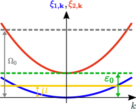
Figure 1: (color online) Illustration of the two-band model used in this work. Two electron-like parabolic and concentric bands are displaced by an energy $\varepsilon_{0}>0$. Their occupations are controlled by the chemical potential $\mu>0$. When $\mu$ becomes larger than $\varepsilon_{0}$, the second band becomes populated, signaling a Lifshitz transition (LT).

The pairing interaction is described by the matrix $V_{ij}$ and contains both (momentum-independent) intra-band pairing, $V_{11}$ and $V_{22}$ which do not need to be necessarily equal, and inter-band pairing, $V_{12}=V_{21}$. As a result, the isotropic SC gap $\Delta_{i}$ in band $i$ is given by:

$$\Delta_{i}=-\sum\limits_{\mathbf{k},j}V_{ij}\left\langle c_{j,-\mathbf{k}\downarrow}c_{j,\mathbf{k}\uparrow}\right\rangle\text{ .}$$ (2)

yielding the usual mean-field Hamiltonian:

$$H_{0}= \sum\limits_{\mathbf{k},i,\sigma}\xi_{i,\mathbf{k}}\,c_{i,\mathbf{k}\sigma}^{{\dagger}}c_{i,\mathbf{k}\sigma}$$

$$-\sum\limits_{\mathbf{k},i}\left(\Delta_{i}\,c_{i,\mathbf{k}\uparrow}^{{\dagger}}c_{i,-\mathbf{k}\downarrow}^{{\dagger}}+h.c.\right)\text{ ,}$$ (3)

Before introducing disorder, we rederive the results for $T_{c}$ of a clean two-band system across a LT (see also Ref. Fernandes13 and references therein). Introducing the Nambu spinor $\hat{\psi}_{\mathbf{k}}^{\dagger}=\left(c_{1,\mathbf{k}\uparrow}^{{\dagger}}\,c_{1,-\mathbf{k}\downarrow}\,c_{2,\mathbf{k}\uparrow}^{{\dagger}}\,c_{2,-\mathbf{k}\downarrow}\right)$, we can readily obtain the normal and anomalous Green’s functions of band $i$, $\mathcal{G}_{i}$ and $\mathcal{F}_{i}$, which appear in the Nambu’s Green’s function $\hat{\mathcal{G}}_{0}$ as:

$$\hat{\mathcal{G}}_{0}(\mathbf{k},\omega_{n})=\begin{pmatrix}\mathcal{G}_{1,0}&\mathcal{F}_{1,0}&0&0\\ \mathcal{F}_{1,0}&-\mathcal{G}_{1,0}^{*}&0&0\\ 0&0&\mathcal{G}_{2,0}&\mathcal{F}_{2,0}\\ 0&0&\mathcal{F}_{2,0}&-\mathcal{G}_{2,0}^{*}\end{pmatrix}\text{ ,}$$ (4)

We find:

$$\mathcal{G}_{i,0}(\mathbf{k},\omega_{n})=-\frac{i\omega_{n}+\xi_{i,\mathbf{k}}}{\omega_{n}^{2}+\xi_{i,\mathbf{k}}^{2}+\Delta_{i}^{2}}\text{ ,}$$ (5)

and

$$\mathcal{F}_{i,0}(\mathbf{k},\omega_{n})=\frac{\Delta_{i}}{\omega_{n}^{2}+\xi_{i,\mathbf{k}}^{2}+\Delta_{i}^{2}}\text{ .}$$ (6)

The latter is related to the pair expectation value, $\left\langle c_{i,-\mathbf{k}\downarrow}c_{i,\mathbf{k}\uparrow}\right\rangle=T\sum_{n}\mathcal{F}_{i,0}(\mathbf{k},\omega_{n})$, from which we can derive the gap equation:

$$\Delta_{i}=\pi T\sum\limits_{j,n}\lambda_{ij}\Delta_{j}\left\langle\frac{1}{\omega_{n}^{2}+\xi^{2}+\Delta_{j}^{2}}\right\rangle_{j}^{\Omega_{0}}\!\!\text{ .}$$ (7)

Here, we introduced the dimensionless coupling constants $\lambda_{ij}=-\rho_{j,0}V_{ij}$, such that positive and negative $\lambda_{ij}$ correspond to attraction and repulsion, respectively. We also defined the notation:

$$\left\langle\mathcal{O}(\xi)\right\rangle_{i}^{\xi_{c}}\equiv\frac{1}{\pi\rho_{i,0}}\int\limits_{W_{i}}^{\xi_{c}}d\xi\rho_{i}(\xi)\mathcal{O}(\xi)\text{ ,}$$ (8)

where $\mathcal{O}(\xi)$ is an arbitrary function of energy, $\xi_{c}$ denotes the upper cutoff of the integral, and $W_{i}$ denotes the bottom of band $i$. In the gap equation, the upper limit of the integration corresponds to the energy cutoff of the pairing interaction, $\Omega_{0}$, which plays a similar role as the Debye frequency in the standard BCS approach. Finally, $\rho_{i}(\xi)$ is the density of states per spin of band $i$, and $\rho_{i,0}\equiv\rho_{i}(W_{i}+\varepsilon_{0})$. Since we have parabolic bands, $\rho_{i}(\xi)=\frac{m_{i}}{2\pi}$ for the 2D case and $\rho_{i}(\xi)=\frac{(2m_{i})^{3/2}\sqrt{\varepsilon_{0}}}{4\pi^{2}}\sqrt{\frac{\xi-W_{i}}{\varepsilon_{0}}}$ for the 3D case, yielding $\rho_{i,0}=\frac{m_{i}}{2\pi}$ and $\rho_{i,0}=\frac{(2m_{i})^{3/2}\sqrt{\varepsilon_{0}}}{4\pi^{2}}$, respectively. The linearized gap equation follows directly from Eq. (7):

$$\begin{pmatrix}\Delta_{1}\\ \Delta_{2}\end{pmatrix}=\begin{pmatrix}\lambda_{11}&\lambda_{12}\\ \lambda_{21}&\lambda_{22}\end{pmatrix}\hat{A}_{\mathrm{clean}}(\mu,T_{c})\begin{pmatrix}\Delta_{1}\\ \Delta_{2}\end{pmatrix}\text{ .}$$ (9)

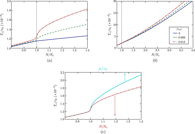
Figure 2: (color online) Phase diagram of the clean two-band SC: the first two panels show $T_{c}$ as function of the occupation number $N$ for (a) 2D bands and (b) 3D bands, for several values of the parameter $\lambda_{12}$. In panel (c), we compare $T_{c}$ as a function of $N$ with $T_{c}$ as a function of the chemical potential $\mu(T_{c})$ for the 2D case with $|\lambda_{12}|=0.013$. In all panels, $\lambda_{11}=\lambda_{22}=0.13$ and $\rho_{2,0}=\rho_{1,0}$. Note that $T_{c}$ is normalized by the energy displacement between the bands $\varepsilon_{0}$ and $N$ is normalized by the critical occupation number $N_{c}$ at which the LT takes place.

where $\hat{A}_{\mathrm{clean}}$ has matrix elements:

$$\left(\hat{A}_{\mathrm{clean}}\right)_{ij} =\delta_{ij}\pi T_{c}\sum\limits_{n}\left\langle\frac{1}{\omega_{n}^{2}+\xi^{2}}\right\rangle_{i}^{\Omega_{0}}$$

$$=\delta_{ij}\,\frac{\pi}{2}\left\langle\frac{1}{\xi}\,\text{tanh}\left(\frac{\xi}{2T_{c}}\right)\right\rangle_{i}^{\Omega_{0}}\text{ .}$$ (10)

Equation (9) defines an eigenvalue problem. $T_{c}$, as a function of the chemical potential $\mu$, is determined when the largest eigenvalue of $\hat{\lambda}\hat{A}_{\mathrm{clean}}$ equals $1$, where $(\hat{\lambda})_{ij}=\lambda_{ij}$. This is given by:

$$\prod_{i=1,2}\left[\left(\hat{A}_{\mathrm{clean}}\right)_{ii}\det\left(\hat{\lambda}\right)-\lambda_{\bar{i}\bar{i}}\right]=\lambda_{12}\lambda_{21}\text{ ,}$$ (11)

as long as $\det\left(\hat{\lambda}\right)=\lambda_{11}\lambda_{22}-\lambda_{12}\lambda_{21}\neq 0$. Here, we introduced the notation $\bar{i}=1(2)$ for $i=2(1)$. It is clear that the equations depend only on the product $\lambda_{12}\lambda_{21}$, i.e. only on the square of the inter-band interaction $V_{12}^{2}$. As a result, $T_{c}(\mu)$ is independent of whether the inter-band pairing interaction is repulsive or attractive Fernandes13 ; Valentinis16 . On the other hand, the sign of the off-diagonal term $\lambda_{12}$ (which by definition is the same as the sign of $\lambda_{21}$ and the opposite of $V_{12}$) determines the eigenvector corresponding to the largest eigenvalue of $\hat{\lambda}\hat{A}$ . When $\lambda_{12}>0$, this eigenvector is such that $\Delta_{1}$ and $\Delta_{2}$ have the same sign, corresponding to a conventional $s^{++}$ SC state. When $\lambda_{12}<0$, $\Delta_{1}$ and $\Delta_{2}$ acquire opposite signs, corresponding to an unconventional $s^{+-}$ SC state

It is important to note that the chemical potential $\mu$ that appears in the gap equation is not the $T=0$ chemical potential, but actually $\mu(T_{c})$. Close to the LT, because the Fermi energy is small, $\mu(T_{c})$ can be different than $\mu(0)$ Chubukov16 . To avoid this issue, one can express the superconducting transition temperature as function of the total number of electrons in the system, $N$, which is given by:

$$N =2\sum\limits_{\mathbf{k}}\left[1-T_{c}\sum\limits_{j,n}\frac{\xi_{j,\mathbf{k}}}{\omega_{n}^{2}+\xi_{j,\mathbf{k}}^{2}}\right]$$

$$=2\pi\mathcal{V}\sum\limits_{j=1}^{2}\rho_{j,0}\left\langle\frac{1}{1+e\,^{\xi/T_{c}}}\right\rangle_{j}^{\Lambda}\text{ ,}$$ (12)

where $\mathcal{V}$ denotes the total volume of the system (or total area, in the 2D case). Note that, here, the upper integration cutoff is the bandwidth $\Lambda$.

The numerical solution of Eqs. (9) and (12) is straightforward, and gives $T_{c}(N)$ as shown in Figs.2 (a) and (b) for the 2D and 3D cases, respectively. In these figures, $T_{c}$ is normalized by $\varepsilon_{0}$ and $N$ is normalized by the critical value $N_{c}$ at which the LT takes place, which corresponds to $\mu(0)=\varepsilon_{0}$. For this particular figure, we used the same density of states for both bands ($\rho_{1,0}=\rho_{2,0}$), we set the interaction cutoff and the bandwidth to the same value $\Omega_{0}=\Lambda=5\varepsilon_{0}$, and considered dominant intra-band interactions $\lambda_{11}=\lambda_{22}=0.13$ with subleading inter-band interactions, $|\lambda_{12}|\ll\lambda_{11}$. The main feature is the enhancement of $T_{c}$ in the vicinity of the LT. Such an enhancement is sharper for 2D bands since in this case the density of states is discontinuous as the chemical potential crosses the band edge.

II.2 Asymptotic solution

To set the stage for the analytic investigations of the dirty case, here we derive an analytic asymptotic expression for $T_{c}(\mu)$ in the particular case of 2D bands. Note that, as discussed in Ref. Trevisan_Schutt_Fernandes and illustrated in Fig. 2, the case of 3D bands is qualitatively similar than the 2D case. The main quantitative differences arise from the fact that the density of states of the 3D bands vanish smoothly at the band edge. Moreover, because the behavior of the curves $T_{c}(\mu)$ and $T_{c}(N)$ are very similar, as illustrated in Fig.2(c), we will focus on the former.

Returning to the matrix elements $\left(\hat{A}_{\mathrm{clean}}\right)_{ij}$ in Eq.(10), it is clear that the main effect of the LT is on the lower integration limits $W_{i}$. Recall that $W_{1}=-\mu$ is the bottom of band $1$ and $W_{2}=-\mu+\varepsilon_{0}$ is the bottom of band $2$. If the chemical potential was such that $\mu\gg\Omega_{0}$, the problem would be in the high-density limit, and we would recover the usual BCS result $\left(\hat{A}_{\mathrm{clean}}\right)_{ij}=\delta_{ij}\left(\frac{\rho_{i,F}}{\rho_{i,0}}\right)\ln\left(\frac{1.13\Omega_{0}}{T_{c}}\right)$, where $\rho_{i,F}$ is the density of states at the Fermi level. To capture the behavior near the LT, we first perform the energy integration and obtain:

$$\left(\hat{A}_{\mathrm{clean}}\right)_{ii}=T_{c}\sum_{n}\frac{1}{\omega_{n}}\left[\text{arctan}\left(\frac{\Omega_{0}}{\omega_{n}}\right)-\text{arctan}\left(\frac{W_{i}}{\omega_{n}}\right)\right]\text{ .}$$ (13)

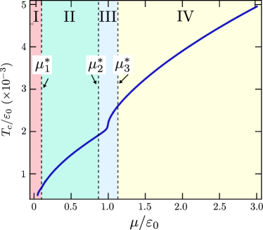
Figure 3: (color online) Regions of the $(\mu,T)$ phase diagram for the calculation of the asymptotic behavior of $T_{c}(\mu)$ in the clean and dirty regimes. The size of the regions are exaggerated for schematic purposes. The precise definition of each region is given in the main text.

For each band, there are two different asymptotic regimes in which the Matsubara sum can be evaluated analytically: $\left|W_{i}\right|\ll T_{c}$ and $\left|W_{i}\right|\gg T_{c}$ (note that, in our weak-coupling approach, $\Omega_{0}\gg T_{c}$ always). This defines $4$ regions in the $\left(\mu,T_{c}\right)$ phase diagram, as schematically shown in Fig. 3:

• In region I, we have $-W_{1}<T_{c}$ and $W_{2}>T_{c}$. This region corresponds to $\mu<\mu_{1}^{*}$, with $\mu_{1}^{*}\sim T_{c}\left(\mu_{1}^{*}\right)$.

• In region II, we have $-W_{1}>T_{c}$ and $W_{2}>T_{c}$. This region corresponds to $\mu_{1}^{*}<\mu<\mu_{2}^{*}$, with $\mu_{2}^{*}\sim\varepsilon_{0}-T_{c}\left(\mu_{2}^{*}\right)$.

• In region III, we have $-W_{1}>T_{c}$ and $\left|W_{2}\right|<T_{c}$. This region corresponds to $\mu_{2}^{*}<\mu<\mu_{3}^{*}$, with $\mu_{3}^{*}\sim\varepsilon_{0}+T_{c}\left(\mu_{3}^{*}\right)$.

• In region IV, we have $-W_{1}>T_{c}$ and $-W_{2}>T_{c}$. This region corresponds to $\mu>\mu_{3}^{*}$.

As shown in Appendix A, we find the diagonal matrix elements in each region:

$$\left(\hat{A}_{\mathrm{clean}}\right)_{11}\sim\frac{1}{2}\begin{cases}\ln\left(\frac{\kappa\Omega_{0}}{T_{c}}\right)+\frac{\mu}{2T_{c}}\text{,}&\text{ region I}\\[14.22636pt] \ln\left(\frac{\kappa^{2}\Omega_{0}\mu}{T_{c}^{2}}\right)\text{,}&\text{ otherwise}\end{cases}\text{ ,}$$ (14)

and

$$\left(\hat{A}_{\mathrm{clean}}\right)_{22}\sim\frac{1}{2}\begin{cases}\ln\left(\frac{\Omega_{0}}{\varepsilon_{0}-\mu}\right)\text{,}&\text{ regions I and II}\\[14.22636pt] \ln\left(\frac{\kappa\Omega_{0}}{T_{c}}\right)+\frac{\left(\mu-\varepsilon_{0}\right)}{2T_{c}}\text{,}&\text{ region III}\\[14.22636pt] \ln\left(\frac{\kappa^{2}\Omega_{0}(\mu-\varepsilon_{0})}{T_{c}^{2}}\right)\text{,}&\text{ region IV}\end{cases}\text{,}$$ (15)

where $\kappa=2\mathrm{e}^{\gamma}/\pi\approx 1.13$, with $\gamma$ denoting Euler’s constant. Solving the gap equation (11) now corresponds to solving a simple transcendental equation, since $\left(\hat{A}_{\mathrm{clean}}\right)_{11}$ and $\left(\hat{A}_{\mathrm{clean}}\right)_{22}$ are analytic functions of $\mu$ and $T_{c}$. This is in contrast to the full numerical solution, which requires numerical evaluation of Matsubara sums or energy integrations.

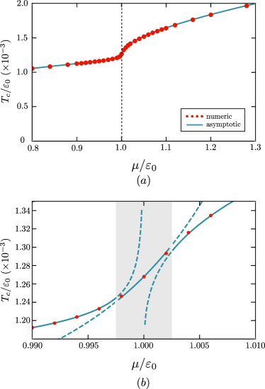
Figure 4: (color online) Comparison between the numerical (symbols) and asymptotic analytical results (solid curve) for $T_{c}$, as function of the chemical potential $\mu$, for the 2D clean system across the Lifshitz transition at $\mu=\varepsilon_{0}$. Panel (b) is a zoom of panel (a) that highlights the very narrow range of $\mu$ for which the asymptotic solutions start to fail (gray dashed area). The parameters used here are the same as in Fig. 2(c).

In Fig. 4(a), we compare the asymptotic and numerical results for the 2D clean system, demonstrating their excellent agreement. It is important to emphasize that, due to its very nature, the asymptotic solution is not continuous across the boundaries defining the different regions. In fact, as shown in Fig. 4(b), some of the asymptotic solutions show diverging behavior near the boundaries. Importantly, as highlighted in the same figure, the ranges of $\mu$ for which the asymptotic solutions do not behave well are very small – in fact, they are too small to be shown in the scale of panel (a), and are thus omitted in that plot. Although in the clean case the advantages of the asymptotic approach may seem rather minor, it will play an important role in gaining insight to the behavior of the dirty system.

III Dirty two-band superconductor

The effects of impurities in our model are captured by adding to Eq.(3) the impurity Hamiltonian

$$H_{\mathrm{imp}}=\sum\limits_{\mathbf{k},\mathbf{k^{\prime}},\sigma}\sum\limits_{\alpha,\beta}W_{\alpha\beta}(\mathbf{k}-\mathbf{k^{\prime}})c_{\alpha,\mathbf{k}\sigma}^{{\dagger}}c_{\beta,\mathbf{k^{\prime}}\sigma}\text{ ,}$$ (16)

where $W_{\alpha\beta}(\mathbf{q})$ is the impurity potential. Because we are interested in the case of incipient bands, we focus on small-momentum impurity scattering. For simplicity, we consider equal intra-band impurity potential, $v\equiv W_{11}\left(0\right)=W_{22}\left(0\right)$, and inter-band impurity potential $u\equiv W_{12}\left(0\right)=W_{21}(0)$.

To proceed, we consider the standard self-consistent Born approximation, as illustrated in Fig.5. The Green’s function in Nambu space is given self-consistently by Dyson’s equation:

$$\hat{\mathcal{G}}^{-1}(\mathbf{k},\omega_{n})=\hat{\mathcal{G}}_{0}^{-1}(\mathbf{k},\omega_{n})-\hat{\Sigma}(\mathbf{k},\omega_{n})\text{ .}$$ (17)

where the matrix $\hat{\mathcal{G}}_{0}(\mathbf{k},\omega_{n})$ is the Green’s function of the clean system shown above in Eq.(4), and $\hat{\Sigma}(\mathbf{k},\omega_{n})$ is the impurity self-energy:

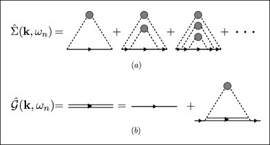
Figure 5: Panel (a) shows the diagrammatic expansion for the self-energy in the self-consistent Born approximation. Panel (b) shows the Dyson’s equation for the total Green’s function according to the self-consistent Born approximation. The solid single lines represent $\hat{\mathcal{G}}_{0}(\mathbf{k},\omega_{n})$, while the dashed lines refer to the impurity potential $\hat{W}_{\mathbf{k},\mathbf{k^{\prime}}}$.

$$\hat{\Sigma}(\mathbf{k},\omega_{n})=n_{\mathrm{imp}}\int\frac{d^{d}k^{\prime}}{(2\pi)^{d}}\hat{W}_{\mathbf{k^{\prime}}-\mathbf{k}}\hat{\mathcal{G}}(\mathbf{k^{\prime}},\omega_{n})\hat{W}_{\mathbf{k}-\mathbf{k^{\prime}}}\text{ ,}$$ (18)

Here, $n_{\mathrm{imp}}$ is the impurity concentration and $\hat{W}_{\mathbf{k},\mathbf{k^{\prime}}}$ represents the impurity potential in Nambu space,

$$\hat{W}_{\mathbf{k},\mathbf{k^{\prime}}}=\begin{pmatrix}v&0&u&0\\ 0&-v&0&-u\\ u&0&v&0\\ 0&-u&0&-v\end{pmatrix}\text{ .}$$ (19)

$\hat{\mathcal{G}}$ can be parametrized by the same matrix structure as $\hat{\mathcal{G}}_{0}$ in Eq.(4), but with renormalized Matsubara frequencies $\tilde{\omega}_{n,j}$, energy dispersions $\tilde{\xi}_{j,\mathbf{k}}\equiv\xi_{j,\mathbf{k}}+h_{n,j}$ and SC gaps $\tilde{\Delta}_{j}$. As a result, we find the following set of self-consistent equations

$$\tilde{\omega}_{n,i} =\omega_{n}+\sum\limits_{j}\frac{\tau_{ij}^{-1}\tilde{\omega}_{n,j}}{2}\left\langle\frac{1}{\tilde{\omega}_{n,j}^{2}+\left(\xi+h_{n,j}\right)^{2}+\tilde{\Delta}_{j}^{2}}\right\rangle_{j}^{\Lambda}\text{ ,}$$ (20)

$$\tilde{\Delta}_{i} =\Delta_{i}+\sum\limits_{j}\frac{\tau_{ij}^{-1}\tilde{\Delta}_{j}}{2}\left\langle\frac{1}{\tilde{\omega}_{n,j}^{2}+\left(\xi+h_{n,j}\right)^{2}+\tilde{\Delta}_{j}^{2}}\right\rangle_{j}^{\Lambda}\text{ ,}$$ (21)

$$h_{n,i} =-\sum\limits_{j}\frac{\tau_{ij}^{-1}}{2}\left\langle\frac{\xi+h_{n,j}}{\tilde{\omega}_{n,j}^{2}+\left(\xi+h_{n,j}\right)^{2}+\tilde{\Delta}_{j}^{2}}\right\rangle_{j}^{\Lambda}\text{ .}$$ (22)

where we introduced the impurity scattering rates $\tau_{ij}^{-1}=2\pi n_{\mathrm{imp}}\rho_{j,0}\left(|v|^{2}\delta_{i,j}+|u|^{2}\delta_{\bar{i},j}\right)$, with $\bar{i}=1(2)$ if $i=2(1)$. We also introduced here the bandwidth $\Lambda$, which we set to be the same for both bands, for simplicity. Since we are interested in the linearized gap equation, we can take the limit of $\tilde{\Delta}_{j}\rightarrow 0$ in the equations above. The linear relationship between $\tilde{\Delta}_{i}$ and $\Delta_{i}$ is then given by:

$$\begin{pmatrix}\tilde{\Delta}_{1}\\ \tilde{\Delta}_{2}\end{pmatrix}=\frac{1}{D_{n}}\hat{M}_{n}\begin{pmatrix}\Delta_{1}\\ \Delta_{2}\end{pmatrix}\text{ ,}$$ (23)

where the matrix $\hat{M}$ is:

$$\left(\hat{M}_{n}\right)_{ij} =\left(1-\frac{\tau_{\bar{i}\bar{i}}^{-1}}{2}\left\langle\frac{1}{\tilde{\omega}_{n,\bar{i}}^{2}+\left(\xi+h_{n,\bar{i}}\right)^{2}}\right\rangle_{\bar{i}}^{\Lambda}\right)\delta_{i,j}$$

$$+\frac{\tau_{ij}^{-1}}{2}\left\langle\frac{1}{\tilde{\omega}_{n,j}^{2}+\left(\xi+h_{n,j}\right)^{2}}\right\rangle_{j}^{\Lambda}\delta_{\bar{i},j}$$ (24)

and $D_{n}\equiv\text{det}(\hat{M}_{n})$ is its determinant, given explicitly by:

$$D_{n} =1-\sum\limits_{i}\frac{\tau_{ii}^{-1}}{2}\left\langle\frac{1}{\tilde{\omega}_{n,i}^{2}+\left(\xi+h_{n,i}\right)^{2}}\right\rangle_{i}^{\Lambda}+$$

$$+\frac{\det\left(\hat{\tau}^{-1}\right)}{4}\prod_{i}\left\langle\frac{1}{\tilde{\omega}_{n,i}^{2}+\left(\xi+h_{n,i}\right)^{2}}\right\rangle_{i}^{\Lambda}$$ (25)

with $\left(\hat{\tau}^{-1}\right)_{ij}\equiv\tau_{ij}^{-1}$. To calculate $T_{c}$, we once again relate the pair expectation value with the anomalous Green’s function, $\left\langle c_{i,-\mathbf{k}\downarrow}c_{i,\mathbf{k}\uparrow}\right\rangle=T\sum_{n}\mathcal{F}_{i}(\mathbf{k},\omega_{n})$. Using the relationship between $\tilde{\Delta}_{i}$ and $\Delta_{i}$ above, we obtain a gap equation of the same form of Eq.(9), but with the matrix $\hat{A}_{\mathrm{clean}}\rightarrow\hat{A}_{\mathrm{dirty}}$. The new matrix is given by:

$$\left(\hat{A}_{\mathrm{dirty}}\right)_{ij}=\pi T_{c}\sum\limits_{n}\frac{B_{i}^{(n)}}{D_{n}}\left(\delta_{ij}+C_{ij}^{(n)}\right)$$ (26)

where

$$B_{i}^{(n)}=\left\langle\frac{1}{\tilde{\omega}_{n,i}^{2}+(\xi+h_{n,i})^{2}}\right\rangle_{i}^{\Omega_{0}}\text{ ,}$$ (27)

and

$$C_{ij}^{(n)} =-\delta_{i,j}\,\frac{\tau_{\bar{i}\bar{i}}^{-1}}{2}\left\langle\frac{1}{\tilde{\omega}_{n,\bar{i}}^{2}+\left(\xi+h_{n,\bar{i}}\right)^{2}}\right\rangle_{\bar{i}}^{\Lambda}$$

$$+\delta_{\bar{i},j}\,\frac{\tau_{ij}^{-1}}{2}\left\langle\frac{1}{\tilde{\omega}_{n,j}^{2}+\left(\xi+h_{n,j}\right)^{2}}\right\rangle_{j}^{\Lambda}\text{ .}$$ (28)

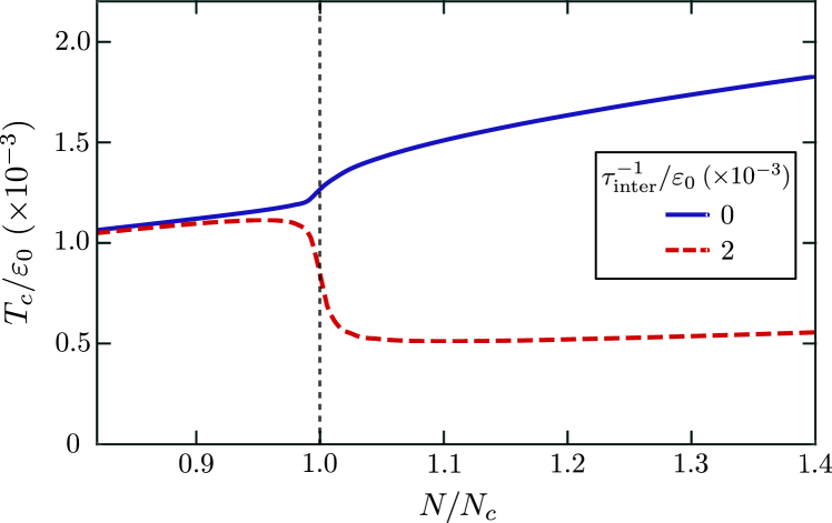
Figure 6: (color online) Superconducting transition temperature $T_{c}$ as a function of the occupation number $N$ of a dirty two-band SC with 2D bands. The dashed line corresponds to finite inter-band impurity scattering (dirty system), whereas the solid line corresponds to the clean system. The parameters are the same as in Fig. 2(c); here, the intra-band impurity scattering is set to zero.

It is clear that, when $\hat{\tau}=0$, $\hat{A}_{\mathrm{dirty}}$ reduces to $\hat{A}_{\mathrm{clean}}$. Similarly, the equation relating the chemical potential $\mu$ to the total number of electrons $N$ is modified to:

$$N=2\sum\limits_{\mathbf{k}}\left[1-T_{c}\sum\limits_{j,n}\frac{\left(\xi_{j,\mathbf{k}}+h_{n,j}\right)}{\tilde{\omega}_{n,j}^{2}+\left(\xi_{j,\mathbf{k}}+h_{n,j}\right)^{2}}\right]$$ (29)

Solving Eqs.(20) and (22) together with the eigenvalue problem and the number equation, we can determine $T_{c}(N)$ numerically. The results, which were presented in Ref.Trevisan_Schutt_Fernandes , reveal a pronounced suppression of $T_{c}$ at the Lifshitz transition in the case of dominant attractive intra-band pairing and sub-dominant repulsive inter-band pairing. In the case of sub-dominant attractive inter-band pairing, the suppression is much milder. These results are reproduced for completeness in Fig. 6.

While Ref.Trevisan_Schutt_Fernandes discussed in details the implications of this numerical result for the understanding of the phase diagrams of SrTiO₃ and LaAlO₃/SrTiO₃, here we are interested in the mechanisms behind this suppression of $T_{c}$ near the Lifshitz transition, and its generalization to a wider parameter regime that goes beyond those applicable to the materials above. To achieve this goal, we develop now an analytical asymptotic solution of $T_{c}$ in two different regimes: the dilute regime and the high-density regime.

IV Asymptotic solution of the dirty two-band superconductor

Our goal here is to analytically study $T_{c}\left(\hat{\tau}^{-1}\right)$ in the different regions of the two-band superconductor $(\mu,T_{c})$ phase diagram shown in Fig. 3. To avoid cumbersome notations, we denote $T_{c}\left(\hat{\tau}^{-1}=0\right)\equiv T_{c,0}$, and $\hat{A}_{\mathrm{dirty}}\equiv\hat{A}_{d}$, $\hat{A}_{\mathrm{clean}}=\hat{A}_{c}$. Since the general function for $T_{c}\left(\hat{\tau}^{-1}\right)$ has no analytic form, we will focus here on the behavior for weak disorder and compute $\partial T_{c}/\partial\tau_{ij}^{-1}$. This quantity can be conveniently calculated applying Hellmann-Feynman theorem (see for instance Refs. Rainer73 ; Kang16 ). Recall that $T_{c}$ is given by the solution of the linearized gap equation $\hat{\Delta}=\left(\hat{\lambda}\hat{A}_{d}\right)\hat{\Delta}$. Let $\alpha\left(T\right)$ be the largest eigenvalue of $\left(\hat{\lambda}\hat{A}_{d}\right)$ for a given temperature $T$ and $\alpha_{0}\left(T\right)$ the largest eigenvalue of $\left(\hat{\lambda}\hat{A}_{c}\right)$. Denote by $\left\langle\alpha_{L}^{(0)}\right|$ and $\left|\alpha_{R}^{(0)}\right\rangle$ the left and right eigenvectors corresponding to $\alpha_{0}\left(T\right)$. Hellmann-Feynman theorem states that

$$\left.\frac{\partial\alpha}{\partial\tau_{ij}^{-1}}\right|_{\tau_{ij}^{-1}=0}=\frac{\left\langle\alpha_{L}^{(0)}\left|\frac{\partial\left(\hat{\lambda}\hat{A}_{d}\right)}{\partial\tau_{ij}^{-1}}\right|\alpha_{R}^{(0)}\right\rangle}{\left\langle\alpha_{L}^{(0)}\left|\alpha_{R}^{(0)}\right.\right\rangle}$$ (30)

Note that, because $\hat{\lambda}\hat{A}_{d}$ is generally non-symmetric, we need to introduce both left and right eigenvectors. Recall that we focus here in the case of fixed chemical potential $\mu$. Since $\alpha(T_{c})=1$, using Maxwell relations, we obtain Rainer73 ; Kang16 :

$$\left.\frac{\partial T_{c}}{\partial\tau_{ij}^{-1}}\right|_{\tau_{ij}^{-1}=0}=-\frac{\left\langle\alpha_{L}^{(0)}\left|\frac{\partial\left(\hat{\lambda}\hat{A}_{d}\right)}{\partial\tau_{ij}^{-1}}\right|\alpha_{R}^{(0)}\right\rangle}{\left\langle\alpha_{L}^{(0)}\left|\alpha_{R}^{(0)}\right.\right\rangle}\frac{1}{\left.\left(\partial\alpha_{0}/\partial T\right)\right|_{T=T_{c}}}\text{ .}$$ (31)

Our goal here is to compare the changes in $T_{c}$ promoted by impurity scattering in the high-density and dilute regimes.

IV.1 High-density regime

We first discuss the high-density regime, i.e. when the system is far from the Lifshitz transition, and the chemical potential is away from the band edge, $\mu\gg\left\{\Omega_{0},\varepsilon_{0}\right\}$. This is the parameter regime most commonly studied in BCS-type approaches to two-band superconductivity. We will recover here several results previously published in the literature Golubov97 ; Efremov11 ; Mishra13 , but also set the stage for the analysis near the LT.

Because $\mu\gg\left\{\Omega_{0},\varepsilon_{0}\right\}$, the lower cutoff of the energy integrals (8) is modified according to:

$$\left\langle\mathcal{O}(\xi)\right\rangle_{i}^{\xi_{c}}\equiv\frac{\rho_{i,F}}{\pi\rho_{i,0}}\int\limits_{-\xi_{c}}^{\xi_{c}}d\xi\,\mathcal{O}(\xi)$$ (32)

where $\xi_{c}$ can assume the values $\Omega_{0}$ or $\Lambda$, and we replaced the density of states by its value at the Fermi level, $\rho_{i,F}\equiv\rho_{i}(\xi_{F})$. In this regime, we can also neglect the renormalization $h_{n,i}$ of the band dispersions. The integrals that appear in the definitions of $\tilde{\omega}_{n}$ and $\hat{A}_{d}$ can then be computed in a straightforward way:

$$\left\langle\frac{1}{\tilde{\omega}_{n,i}^{2}+\xi^{2}}\right\rangle_{i}^{\Omega_{0}}=\left\langle\frac{1}{\tilde{\omega}_{n,i}^{2}+\xi^{2}}\right\rangle_{i}^{\Lambda}=\frac{\rho_{i,F}}{\rho_{i,0}|\tilde{\omega}_{n,i}|}$$ (33)

As a result, the self-consistent equation for $\tilde{\omega}_{n,i}$ can be solved analytically, yielding:

$$\left|\tilde{\omega}_{n,i}\right|=\left|\omega_{n}\right|+\frac{1}{2}\sum\limits_{j}\tau_{ij}^{-1}\text{ ,}$$ (34)

In the expression above and in the remainder of this section, we renormalize the scattering rates and coupling constants such that $\frac{\rho_{i,F}}{\rho_{i,0}}\,\tau_{ij}^{-1}\rightarrow\tau_{ij}^{-1}$ and $\frac{\rho_{i,F}}{\rho_{i,0}}\,\lambda_{ij}\rightarrow\lambda_{ij}$. This corresponds to using the density of states at the Fermi level $\rho_{i,F}$, instead of $\rho_{i,0}$, in the corresponding definitions, i.e. in this section $\lambda_{ij}=-\rho_{j,F}V_{ij}$ and $\tau_{ij}^{-1}=2\pi n_{\mathrm{imp}}\rho_{j,F}\left(|v|^{2}\delta_{i,j}+|u|^{2}\delta_{\bar{i},j}\right)$.

Thus, the different components of $\left(\hat{A}_{d}\right)_{ij}=\pi T_{c}\sum\limits_{n}\frac{B_{i}^{(n)}}{D_{n}}\left(\delta_{ij}+C_{ij}^{(n)}\right)$ become:

$$\frac{B_{i}^{(n)}}{D_{n}} =\frac{\left(\left|\omega_{n}\right|+\frac{1}{2}\sum\limits_{j}\tau_{\bar{i}j}^{-1}\right)}{\left|\omega_{n}\right|\left(\left|\omega_{n}\right|+\frac{1}{2}\sum\limits_{j}\tau_{j\bar{j}}^{-1}\right)}$$ (35)

$$\frac{B_{i}^{(n)}}{D_{n}}\,C_{ij}^{(n)} =\frac{\left(-\delta_{i,j}\tau_{\bar{i}\bar{i}}^{-1}+\delta_{\bar{i},j}\tau_{i\bar{i}}^{-1}\right)}{2\left|\omega_{n}\right|\left(\left|\omega_{n}\right|+\frac{1}{2}\sum\limits_{j}\tau_{j\bar{j}}^{-1}\right)}$$ (36)

where:

$$D_{n}=\frac{\left|\omega_{n}\right|\left(\left|\omega_{n}\right|+\frac{1}{2}\sum\limits_{j}\tau_{j\bar{j}}^{-1}\right)}{\prod\limits_{i}\left(\left|\omega_{n}\right|+\frac{1}{2}\sum\limits_{j}\tau_{ij}^{-1}\right)}$$ (37)

The Matsubara sums appearing in $\hat{A}_{d}$ can be evaluated using the result:

$$\sum\limits_{n}\frac{1}{|\omega_{n}|+x}\approx\frac{1}{\pi T_{c}}\left[\ln\left(\frac{\Gamma_{c}}{2\pi T_{c}}\right)-\psi\left(\frac{1}{2}+\frac{x}{2\pi T_{c}}\right)\right]\text{ ,}$$ (38)

where $\Gamma_{c}$ is the upper cutoff of the Matsubara sum (which is $\Gamma_{c}=\Omega_{0}\gg T_{c}$ for the $B_{i}^{(n)}$ terms), and $\psi(x)$ is the digamma function. We find that $\hat{A}_{d}$ can be cast in the form:

$$\left(\hat{A}_{d}\right)_{ij}=\delta_{i,j}P_{i}+\delta_{\bar{i},j}Q_{i}$$ (39)

with:

$$P_{i} =\ln\left(\frac{\kappa\Omega_{0}}{T_{c}}\right)-\frac{\rho_{\bar{i},F}}{\rho_{1,F}+\rho_{2,F}}\left[\psi\!\left(\frac{1}{2}+\frac{\tau_{\mathrm{inter}}^{-1}}{2\pi T_{c}}\right)-\psi\!\left(\frac{1}{2}\right)\right]$$ (40)

$$Q_{i} =\frac{\rho_{\bar{i},F}}{\rho_{1,F}+\rho_{2,F}}\left[\psi\!\left(\frac{1}{2}+\frac{\tau_{\mathrm{inter}}^{-1}}{2\pi T_{c}}\right)-\psi\!\left(\frac{1}{2}\right)\right]$$ (41)

where $\tau_{\mathrm{inter}}^{-1}\equiv\frac{1}{2}\left(\tau_{12}^{-1}+\tau_{21}^{-1}\right)$ is the average inter-band impurity scattering and $\kappa\approx 1.13$ is the same constant that appears in Sec.II for the clean case.

It is clear that $\hat{A}_{d}$ depends only on the average inter-band impurity scattering $\tau_{\mathrm{inter}}^{-1}$, i.e. $T_{c}$ is unaffected by intra-band impurity scattering. This is not surprising, since the gaps are isotropic and Anderson’s theorem enforces that intra-band non-magnetic impurity scattering cannot affect superconductivity. Using these expressions, the solution of the gap equations, corresponding to finding the largest eigenvalue of $\left(\hat{\lambda}\hat{A}_{d}\right)$, becomes a transcendental equation that can be solved in a straightforward way.

We now proceed to evaluate $\partial T_{c}/\partial\tau_{\mathrm{inter}}^{-1}$ using Eq. (31). For convenience, we introduce the ratio between the densities of states of the two bands to be $r\equiv\rho_{2,F}/\rho_{1,F}$. By definition, it follows that $\lambda_{12}/\lambda_{21}=\tau_{12}^{-1}/\tau_{21}^{-1}=r$. The largest eigenvalue of the clean gap equation is given by

$$\alpha_{0}=\lambda_{+}\ln\left(\frac{\kappa\Omega_{0}}{T_{c}}\right)$$ (42)

where:

$$\lambda_{+}=\lambda_{0}+\sqrt{\delta\lambda^{2}+\frac{1}{r}\lambda_{12}^{2}}$$ (43)

For simplicity of notation, here we introduced $\lambda_{0}=\frac{1}{2}\left(\lambda_{11}+\lambda_{22}\right)$ and $\delta\lambda=\frac{1}{2}\left(\lambda_{11}-\lambda_{22}\right)$. The right and left eigenvectors are given by:

$$\left|\alpha_{R}^{(0)}\right\rangle=\left(\begin{array}[]{c}\delta\lambda+\sqrt{\delta\lambda^{2}+\frac{1}{r}\lambda_{12}^{2}}\\ \frac{1}{r}\lambda_{12}\end{array}\right)$$ (44)

and:

$$\left\langle\alpha_{L}^{(0)}\right|=\left(\begin{array}[]{c}\delta\lambda+\sqrt{\delta\lambda^{2}+\frac{1}{r}\lambda_{12}^{2}}\\ \lambda_{12}\end{array}\right)^{T}$$ (45)

Note that the relative sign of the two components of the eigenvectors, which correspond to the ratio between the two gaps $\Delta_{1}/\Delta_{2}$, is determined solely by $\mathrm{sgn}\left(\lambda_{12}\right)=\mathrm{sgn}\left(\lambda_{21}\right)$, i.e. $\mathrm{sgn}\left(\Delta_{1}/\Delta_{2}\right)=\mathrm{sgn}\left(\lambda_{12}\right)$. As explained in Section II, this implies that attractive inter-band pairing interaction, $\lambda_{12}>0$, promotes a sign-preserving $s^{++}$ state, whereas repulsive inter-band pairing interaction, $\lambda_{12}<0$, promotes a sign-changing $s^{+-}$ state.

Next, from the definition of $\hat{A}_{d}$ in Eq. (39), we obtain:

$$\left.\frac{\partial\left(\hat{\lambda}\hat{A}_{d}\right)}{\partial\tau_{\mathrm{inter}}^{-1}}\right|_{\tau_{\mathrm{inter}}^{-1}=0} =\frac{1}{\left(1+r\right)}\frac{\pi}{4T_{c,0}}\times$$

$$\left(\begin{array}[]{cc}\lambda_{12}-r\lambda_{11}&-\lambda_{12}+r\lambda_{11}\\ \lambda_{22}-\lambda_{12}&-\lambda_{22}+\lambda_{12}\end{array}\right)$$ (48)

It is straightforward to now compute $\partial T_{c}/\partial\tau_{\mathrm{inter}}^{-1}$ via Eq. (31), using that $\frac{\partial\alpha_{0}}{\partial T_{c}}=-\frac{\lambda_{+}}{T_{c,0}}$. The full expression is long and not very insightful. In the particular case of $r=1$, however, the expression simplifies significantly and we obtain:

$$\left.\frac{\partial T_{c}}{\partial\tau_{\mathrm{inter}}^{-1}}\right|_{\tau_{\mathrm{inter}}^{-1}=0}=-\frac{\pi}{8}\left[1-\frac{\mathrm{sgn}\left(\lambda_{12}\right)}{\sqrt{\left(\frac{\lambda_{11}-\lambda_{22}}{2\lambda_{12}}\right)^{2}+1}}\right]$$ (49)

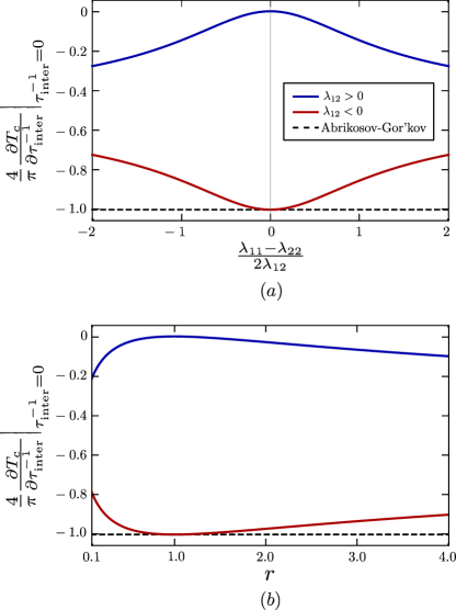
Figure 7: (color online) The rate of suppression of $T_{c}$ by inter-band non-magnetic impurity scattering $\tau_{\mathrm{inter}}^{-1}$, $\left.\frac{\partial T_{c}}{\partial\tau_{\mathrm{inter}}^{-1}}\right|_{\tau_{\mathrm{inter}}^{-1}=0}$ for repulsive ($\lambda_{12}<0$, red curves) and attractive ($\lambda_{12}>0$, blue curves) inter-band pairing interactions, in the high-density regime. In panel (a), the density of states of the two bands are set to be the same, but the intra-band pairing interactions of the two bands, $\lambda_{11}$ and $\lambda_{22}$, are allowed to be different. In panel (b), $\lambda_{11}$ is set to be the same as $\lambda_{22}$, but the two density of states are allowed to be different, with $r=\rho_{2,F}/\rho_{1,F}$. In both panels, the suppression rates are normalized by the magnitude of the Abrikosov-Gor’kov value of $-\pi/4$ corresponding to the suppression rate of $T_{c}$ of a single-band superconductor by magnetic impurity scattering.

This expression reveals important properties of impurity scattering in multi-band superconductors. First, as mentioned above, only inter-band impurity scattering is pair-breaking. Second, this pair-breaking effect takes place generically for both $s^{+-}$ and $s^{++}$ states. Indeed, as long as $\lambda_{11}\neq\lambda_{22}$, $T_{c}$ will be suppressed by impurities regardless of the sign of the inter-band interaction $\lambda_{12}$.

It is clear, however, that the suppression is stronger in the case of repulsive interaction $\lambda_{12}<0$. Compared to the Abrikosov-Gor’kov result for the suppression rate of $T_{c}$ by magnetic impurity scattering in single-band $s$-wave superconductors, $\left(\frac{\partial T_{c}}{\partial\tau_{\mathrm{mag}}^{-1}}\right)_{\mathrm{AG}}=-\frac{\pi}{4}$, it follows that $\left|\frac{\partial T_{c}}{\partial\tau_{\mathrm{inter}}^{-1}}\right|\leq\left|\frac{\partial T_{c}}{\partial\tau_{\mathrm{mag}}^{-1}}\right|$. Note that, according to the expression for the leading eigenvector (44), the magnitudes of the two gaps are necessarily different when $\lambda_{11}\neq\lambda_{22}$, i.e. $\left|\Delta_{1}\right|\neq\left|\Delta_{2}\right|$. In the fine-tuned case of equal intra-band pairing interactions, $\lambda_{11}=\lambda_{22}$, which corresponds to two gaps of same magnitudes, $\left|\Delta_{1}\right|=\left|\Delta_{2}\right|$, $T_{c}$ for the $s^{++}$ state displays no suppression with disorder $\tau_{\mathrm{inter}}^{-1}$, whereas $T_{c}$ for the $s^{+-}$ state displays its maximum suppression. Thus, at the same time that $\lambda_{11}\neq\lambda_{22}$ promotes pair-breaking effects for the $s^{++}$ state, it reduces the pair-breaking effects for the $s^{+-}$ state. This is illustrated in Fig. 7(a).

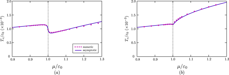
Figure 8: (color online) Comparison between the numerical (symbols) and asymptotic analytical results (solid curves) for $T_{c}$, as function of the chemical potential $\mu$, for the 2D dirty system across the Lifshitz transition at $\mu=\varepsilon_{0}$. The parameters are the same as in Fig. 4 but with $\lambda_{12}<0$ (repulsive inter-band pairing interaction) in panel (a) and $\lambda_{12}>0$ (attractive inter-band pairing interaction) in panel (b). The inter-band impurity scattering $\tau_{\mathrm{inter}}^{-1}$ is set to $\tau_{\mathrm{inter}}^{-1}/\varepsilon_{0}=10^{-3}$.

The difference in the density of states between the two bands, signaled here by $r\neq 1$, plays a similar role as the difference in the intra-band pairing interactions. For instance, if we set $\lambda_{11}=\lambda_{22}$ but consider an arbitrary $r$, we find:

$$\left.\frac{\partial T_{c}}{\partial\tau_{\mathrm{inter}}^{-1}}\right|_{\tau_{\mathrm{inter}}^{-1}=0}=-\frac{\pi}{8}\left[1-\frac{2\sqrt{r}\,\mathrm{sgn}\left(\lambda_{12}\right)}{1+r}\right]$$ (50)

Once again, the suppression of $T_{c}$ for the $s^{++}$ state is minimum (in fact, zero) when $r=1$, whereas the suppression of $T_{c}$ for the $s^{+-}$ state is maximum (and equal to the Abrikosov-Gor’kov value) when $r=1$. This behavior is shown in Fig. 7(b). We emphasize that our analysis reproduces similar conclusions about the role of impurities in multi-band superconductors that have been previously reported elsewhere Golubov97 ; Efremov11 ; Mishra13 .

IV.2 Dilute regime

Our analysis of the high-density regime reveals that impurity pair-breaking effects on $T_{c}$ arise from the inter-band scattering rates, $\tau_{21}^{-1}$ and $\tau_{12}^{-1}$. Thus, in this subsection, to simplify the analysis, we neglect intra-band scattering processes, and set $\tau_{11}^{-1}=\tau_{22}^{-1}=0$. Furthermore, in the same spirit of the previous subsection, we focus on the weak-disorder regime, in which $\tau_{12}^{-1}$ and $\tau_{21}^{-1}$ are small compared to $T_{c,0}$. Finally, we consider 2D bands, in which case the density of states does not depend on the energy. Within these approximations, to linear order in the scattering rates, the renormalized Matsubara frequency in Eq.(20) becomes:

$$\tilde{\omega}_{n,i}=\omega_{n}\left(1+\frac{1}{2\pi}\tau_{i\bar{i}}^{-1}f_{n,\bar{i}}\right)\text{ ,}$$ (51)

where we defined the function:

$$f_{n,i}\equiv\frac{1}{\omega_{n}}\left[\text{arctan}\left(\frac{\Omega_{0}}{\omega_{n}}\right)-\text{arctan}\left(\frac{W_{i}}{\omega_{n}}\right)\right]$$ (52)

Note that, similarly to the previous section, we neglect the renormalization of the band due to disorder, $h_{n,i}$. As shown below, this approximation yields very good agreement between the numerical and the asymptotic results. Evaluating the matrix elements of $\hat{A}_{d}$ in Eq. (26), we find, to linear order in the impurity scattering rate:

$$\hat{A}_{d}=\hat{A}_{c}+\tau_{\mathrm{inter}}^{-1}\delta\hat{A}$$ (53)

Here, $\hat{A}_{c}$ is the clean-case diagonal matrix discussed in Section II.2, $\tau_{\mathrm{inter}}^{-1}\equiv\frac{1}{2}\left(\tau_{12}^{-1}+\tau_{21}^{-1}\right)$ is the average inter-band impurity scattering, and $\delta\hat{A}$ is given by:

$$\left(\delta\hat{A}\right)_{ij}=\frac{1}{2\pi}\left[R_{i}\delta_{ij}+S\left(-\delta_{i,j}+\delta_{\bar{i},j}\right)\right]$$ (54)

with

$$R_{i} =-T_{c}\sum_{n}\left(\frac{\Lambda}{\Lambda^{2}+\omega_{n}^{2}}-\frac{W_{i}}{W_{i}^{2}+\omega_{n}^{2}}\right)f_{n,\bar{i}}\text{,}$$

$$S =T_{c}\sum_{n}f_{n,1}f_{n,2}\text{,}$$ (55)

The expressions above are obtained after two simplifications: we set the density of states of the two bands to be equal, $\rho_{1,0}=\rho_{2,0}$, and consider $\Omega_{0}=\Lambda$. Note that the main results presented here do not rely on these simplifications.

To determine analytic asymptotic expressions for the matrix elements of $\hat{A}_{d}$, we follow the same procedure as in the clean case as outlined in Sec.II.2, and divide the $\left(\mu,T_{c}\right)$ phase diagram in four regions. The calculation is tedious but straightforward; the resulting expressions for $R_{1}$, $R_{2}$, and $S$ are long and shown explicitly in Appendix B. In terms of these expressions, finding $T_{c}$ corresponds to solving the transcendental algebraic equation that comes from the condition that the largest eigenvalue of $\hat{\lambda}\hat{A}_{d}$ equals one (see Appendix C).

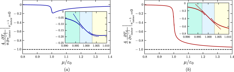
Figure 9: (color online) The rate of suppression of $T_{c}$ by inter-band impurity scattering, $\left.\frac{\partial T_{c}}{\partial\tau_{\mathrm{inter}}^{-1}}\right|_{\tau_{\mathrm{inter}}^{-1}=0}$ for attractive ($\lambda_{12}>0$, panel (a)) and repulsive ($\lambda_{12}<0$, panel (b)) inter-band pairing interactions, in the dilute regime. The insets highlight the asymptotic behaviors across the boundaries of regions II, III, and IV of Fig. 3. In both panels, the suppression rates are normalized by the absolute value of the Abrikosov-Gor’kov suppression rate of $-\pi/4$, corresponding to the case of a single-band superconductor by magnetic impurity scattering. The parameters used here are $\rho_{1,0}=\rho_{2,0}$, $\lambda_{11}=\lambda_{22}$, and $\lambda_{12}=\lambda_{21}$.

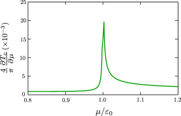
Figure 10: Rate of enhancement of $T_{c}$ by changes in the chemical potential, $\frac{\partial T_{c}}{\partial\mu}$, for the clean 2D system. The parameters are the same as those used in Fig. 9. To make the comparison with that figure more transparent, we also normalize the rate of change of $T_{c}$ by $\pi/4$.

In Fig. 8, we compare the numerical and asymptotic analytical results for the cases of attractive and repulsive inter-band pairing interaction. As in the clean case, the agreement between the two methods is excellent, except in very narrow regions where the asymptotic approximation fails. As in Fig. 4, these regions are too narrow compared to the scale of the plots and are thus not shown in the plots. We note that the agreement between the asymptotic solution and the numerical results near the LT improves as the scattering rates becomes smaller.

In Figs. 9(a) and (b), we plot the analytic asymptotic behavior of $\left.\frac{\partial T_{c}}{\partial\tau_{\mathrm{inter}}^{-1}}\right|_{\tau_{\mathrm{inter}}^{-1}=0}$ as function of the chemical potential for attractive and repulsive inter-band pairing interactions, respectively. Note that the computation of such suppression rate of $T_{c}$ from Eq.(31) is straightforward and details are provided in Appendix C. Similarly to Fig. 7, we normalize $\partial T_{c}/\partial\tau_{\mathrm{inter}}^{-1}$ by the Abrikosov-Gor’kov suppression rate $-\pi/4$. The insets display zooms of the behaviors of the asymptotic solutions near the LT – as in the analysis of previous sections, the asymptotic solutions are not continuous across the boundaries of the different regions of Fig. 3.

The results far from the LT are not surprising: before the LT, when only one band is present, $\partial T_{c}/\partial\tau_{\mathrm{inter}}^{-1}$ is very small, since the second band is sunk below the Fermi level. After the LT, when the second band is no longer incipient, $\partial T_{c}/\partial\tau_{\mathrm{inter}}^{-1}$ approaches the high-density values $-\pi/4$ for repulsive inter-band interaction and $0$ for attractive inter-band pairing interaction.

The interesting behaviors of $\partial T_{c}/\partial\tau_{\mathrm{inter}}^{-1}$ take place in the vicinity of the LT. For $\lambda_{12}<0$, we note a very rapid increase of the magnitude of the suppression rate, despite the fact that the second band is only incipient. On the other hand, for $\lambda_{12}>0$, the magnitude of the suppression rate displays a rather mild maximum when the second band crosses the Fermi level.

The fate of the evolution of $T_{c}$ in the dirty system across the LT depends then on the competition between two opposite effects: the suppression of $T_{c}$ due to the pair-breaking promoted by inter-band impurity scattering, and the enhancement of $T_{c}$ promoted by the new electronic states that become part of the superconducting state once the second band crosses the Fermi level. The latter effect is illustrated in Fig. 10, where $\partial T_{c}/\partial\mu$ obtained from the asymptotic analytical solution of the clean system is shown. Generally, one expects that, for sufficient strong disorder, and for a repulsive inter-band interaction, the former effect wins, such that $T_{c}$ displays a maximum at the LT. This is indeed what we observed in the full solution of the dirty gap equations shown in Fig. 8.

V Concluding remarks

In summary, in this work we developed an asymptotic analytical framework to investigate the behavior of the superconducting transition temperature $T_{c}$ across a Lifshitz transition in a dirty two-band system. Our systematic study unveiled two competing effects that influence the evolution of $T_{c}$. The first effect arises from the fact that the system gains energy via the opening of a superconducting gap in the incipient band, which leads to an enhancement of $T_{c}$ (see Fig. 9(c)). The second effect arises because, as soon as the second band emerges above the Fermi level and the gap becomes non-negligible, pair-breaking effects kick in due to inter-band impurity scattering, resulting in a suppression of $T_{c}$. While the first effect is insensitive to the nature of pairing state – i.e. whether it is an $s^{++}$ state resulting from inter-band attraction or an $s^{+-}$ state resulting from inter-band repulsion – the second effect is much stronger in the case of repulsive pairing interactions. As a result, for an $s^{+-}$ superconductor with significant impurity scattering, $T_{c}$ is expected to be maximum at the LT. Therefore, our results offer important benchmarks to assess indirectly from the shape of the superconducting dome whether a multi-band superconductor is conventional (i.e. driven by attractive pairing interactions only) or unconventional (i.e. driven by repulsive pairing interactions). Note that, if the impurities were magnetic, impurity scattering would be strongly pair-breaking for both attractive and repulsive inter-band interactions (see also Ref. Schimalian15 ). As a result, although an explicit calculation is beyond the scope of this work, one expects a similar behavior of $T_{c}$ across the Lifshitz transition in both cases.

Appendix A Matsubara sums for the clean case

Deriving an analytic expression for the matrix elements $\left(\hat{A}_{\mathrm{clean}}\right)_{ij}$ involves calculating, analytically, Matsubara sums of the type $\sum\limits_{n}\frac{1}{\omega_{n}}\text{arctan}\left(\frac{y}{\omega_{n}}\right)=\frac{\text{sign}(y)}{T_{c}}\,s_{1}\left(\frac{|y|}{T_{c}}\right)$, where the quantity $y$ can assume the values $\Omega_{0}$, $W_{1}=-\mu$ or $W_{2}=-\mu+\varepsilon_{0}$, and

$$s_{1}(|x|)\equiv 2\sum\limits_{n=0}^{\infty}\frac{1}{(2n+1)\pi}\text{arctan}\left(\frac{|x|}{(2n+1)\pi}\right)\text{ .}$$ (56)

We calculate an approximate expression for $s_{1}(|x|)$, taking advantage of the asymptotic behavior of $\text{arctan}\left(\frac{|x|}{(2n+1)\pi}\right)$ in two regimes, $|x|\ll 1$ and $|x|\gg 1$. If $|x|\ll 1$, $\frac{|x|}{(2n+1)\pi}\ll 1$ for all $n$, and a Taylor expansion of $\text{arctan}\left(\frac{|x|}{(2n+1)\pi}\right)$ leads to

$$s_{1}(|x|\ll 1)=2\sum\limits_{l=0}^{\infty}\frac{(-1)^{l}\zeta(2l+2)\left[2^{2l+2}-1\right]}{(2l+1)(2\pi)^{2l+2}}|x|^{2l+1}\text{ ,}$$ (57)

where we used the fact that

$$\sum\limits_{n=0}^{\infty}\frac{1}{\left[(2n+1)\pi\right]^{k}}=\frac{\left(2^{k}-1\right)\zeta(k)}{(2\pi)^{k}}\text{ ,}$$ (58)

with integer $k\geq 2$ and $\zeta(k)$ denoting the Riemann zeta function. The leading term is clearly the $l=0$:

$$s_{1}(|x|\ll 1)\sim\frac{\left|x\right|}{4}$$ (59)

On the other hand, if $|x|\gg 1$, $\frac{|x|}{(2n+1)\pi}\gg 1$ for small values of $n$, but the ratio decreases with increasing $n$, until it eventually behaves as $\frac{|x|}{(2n+1)\pi}\ll 1$ for large enough $n$. Denoting by $N^{*}$ the value of $n$ such that $(2N^{*}+1)\pi=\left|x\right|$, i.e. $N^{*}=\frac{|x|}{2\pi}-\frac{1}{2}$, we approximate $\text{arctan}\left(\frac{|x|}{(2n+1)\pi}\right)$ by its Taylor expansion in powers of $1/|x|$ when $0<n<N^{*}$, and by its Taylor expansion in powers of $|x|$ when $N^{*}+1<n<\infty$. The result is

$$s_{1} (|x|\gg 1)=\sum\limits_{n=0}^{N^{*}}\frac{1}{2n+1}$$

$$-2\sum\limits_{l=0}^{\infty}\frac{(-1)^{l}}{(2l+1)|x|^{2l+1}}\sum\limits_{n=0}^{N^{*}}\left[(2n+1)\pi\right]^{2l}$$

$$+2\sum\limits_{l=0}^{\infty}\frac{(-1)^{l}|x|^{2l+1}}{(2l+1)}\sum\limits_{n=N^{*}+1}^{\infty}\frac{1}{\left[(2n+1)\pi\right]^{2l+2}}\text{.}$$ (60)

The sums over $n$ that appear in Eq.(60) can be evaluated analytically:

$$\sum\limits_{n=0}^{N^{*}}\frac{1}{\left[(2n+1)\pi\right]^{k}}=$$

$$\begin{cases}\frac{(2^{k}-1)\zeta(k)}{(2\pi)^{k}}+\frac{1}{(2\pi)^{k}(|k|+1)}B_{|k|+1}\!\left(1+\frac{|x|}{2\pi}\right)\text{,}&\text{ if }k\leq 0\\[8.5359pt] \frac{1}{2\pi}\left[\psi\left(1+\frac{|x|}{2\pi}\right)-\psi\left(\frac{1}{2}\right)\right]\text{,}&\text{ if }k=1\\[8.5359pt] \frac{(2^{k}-1)\zeta(k)}{(2\pi)^{k}}-\frac{1}{(k-1)!}\!\left(\frac{-1}{2\pi}\right)^{k}\psi^{(k-1)}\!\!\left(1+\frac{|x|}{2\pi}\right)\text{,}&\text{ if }k>1\end{cases}\text{,}$$ (61)

and

$$\sum\limits_{n=N^{*}+1}^{\infty}\frac{1}{\left[(2n+1)\pi\right]^{k}}=$$

$$\frac{1}{(k-1)!}\!\left(\frac{-1}{2\pi}\right)^{k}\psi^{(k-1)}\!\!\left(1+\frac{|x|}{2\pi}\right)\text{ ,}\hskip 8.5359pt\text{ if }k\geq 2\text{,}$$ (62)

where $\psi^{(k)}(x)$, $\psi(x)=\psi^{(0)}(x)$ and $B_{k}(x)$ are, respectively, the polygamma function of $k$-th order, the digamma function, and the Bernoulli polynomials. In the limit $\left|x\right|\gg 1$, a Taylor expansion, up to order $\mathcal{O}\left(\frac{1}{\left|x\right|^{k}}\right)$ leads to:

$$\sum\limits_{n=0}^{N^{*}}\frac{1}{\left[(2n+1)\pi\right]^{k}}\sim$$

$$\begin{cases}\frac{1}{2\pi}\ln\left(\kappa|x|\right)\text{,}&\text{ if }k=1\\[8.5359pt] \frac{(2^{k}-1)\zeta(k)}{(2\pi)^{k}}-\frac{1}{2\pi(k-1)|x|^{k-1}}\text{,}&\text{ if }k\leq 0\text{ or }k>1\end{cases}\text{,}$$ (63)

and

$$\sum\limits_{n=N^{*}+1}^{\infty}\frac{1}{\left[(2n+1)\pi\right]^{k}}\sim\frac{1}{2\pi(k-1)|x|^{k-1}}\text{ ,}\hskip 8.5359pt\text{ if }k\geq 2\text{.}$$ (64)

where we defined the constant $\kappa=2e^{\gamma}/\pi\approx 1.13$, with $\gamma$ denoting Euler’s constant.

Substituting Eqs.(63) and (64) into Eq.(60), we find that its second and third terms result in the same constant $\sum\limits_{l=0}^{\infty}\frac{(-1)^{l}}{\pi(2l+1)^{2}}=\frac{\mathcal{C}}{\pi}$ ($\mathcal{C}\approx 0.92$ is the Catalan’s constant), differing only by a minus sign. Thus, they cancel out, and we obtain:

$$s_{1}(|x|\gg 1)\sim\frac{1}{2}\ln\left(\kappa|x|\right)\text{ .}$$ (65)

To summarize, combining Eqs.(59) and (65), we have

$$s_{1}(|x|)\sim\begin{cases}\frac{|x|}{4}\text{ ,}&\text{ if }|x|\ll 1\\[8.5359pt] \frac{1}{2}\ln\left(\kappa|x|\right)\text{ ,}&\text{ if }|x|\gg 1\end{cases}\text{.}$$ (66)

Note that $s_{1}(|x|\rightarrow 1^{+})\neq s_{1}(|x|\rightarrow 1^{-})$. This is because the asymptotic approach we described begins to fail for $|x|$ of order one, as we can see in Fig.11. As a consequence, the asymptotic expressions for $T_{c}(\mu)$ deviate from the numeric results when $\mu$ approaches the boundaries $\mu_{1}^{*}$, $\mu_{2}^{*}$ and $\mu_{3}^{*}$ of the regions of the phase diagram illustrated in Fig. 3. At these points, either $|W_{1}|$ or $|W_{2}|$ becomes of the order of $T_{c}$.

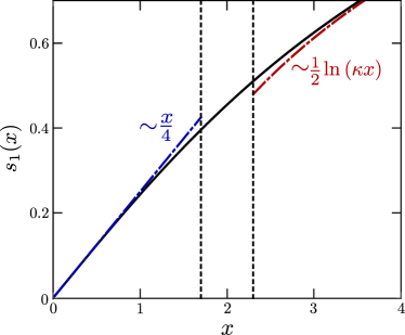
Figure 11: (color online) Numerical and asymptotic solutions for the Matsubara sum (56). The dot-dashed blue and red lines are the asymptotic solutions for $|x|\ll 1$ and $|x|\gg 1$, while the solid line is the numerical result. The dashed vertical lines delimit the region where the asymptotic approximation begins to fail.

Appendix B Matsubara sums for the dirty case

In the case of a dirty two-band SC, there are two distinct types of Matsubara sums that we need to calculate for $\delta\hat{A}$, as shown in Eq. (55). The first are sums of the type:

$$\sum\limits_{n}\frac{1}{\omega_{n}}\text{arctan}\left(\frac{y_{1}}{\omega_{n}}\right)\frac{y_{2}}{y_{2}^{2}+\omega_{n}^{2}}$$

$$=\frac{\text{sign}(y_{1}y_{2})}{T_{c}^{2}}\,s_{2}\left(\frac{|y_{1}|}{T_{c}},\frac{|y_{2}|}{T_{c}}\right)$$ (67)

where we define:

$$s_{2}(|x_{1}|,|x_{2}|)\equiv$$

$$2\sum\limits_{n=0}^{\infty}\frac{1}{(2n+1)\pi}\text{arctan}\!\left(\frac{|x_{1}|}{(2n+1)\pi}\right)\frac{|x_{2}|}{|x_{2}|^{2}+\left[(2n+1)\pi\right]^{2}}\text{,}$$ (68)

The other sum is:

$$\sum\limits_{n}\frac{1}{\omega_{n}^{2}}\text{arctan}\left(\frac{y_{1}}{\omega_{n}}\right)\text{arctan}\left(\frac{y_{2}}{\omega_{n}}\right)$$

$$=\frac{\text{sign}(y_{1}y_{2})}{T_{c}^{2}}s_{3}\left(\frac{|y_{1}|}{T_{c}},\!\frac{|y_{2}|}{T_{c}}\right)$$

where we define:

$$s_{3}(|x_{1}|,|x_{2}|)\equiv$$

$$2\sum\limits_{n=0}^{\infty}\frac{1}{\left[(2n+1)\pi\right]^{2}}\text{arctan}\!\!\left(\!\frac{|x_{1}|}{(2n+1)\pi}\!\right)\text{arctan}\!\!\left(\!\frac{|x_{2}|}{(2n+1)\pi}\!\right)\text{.}$$ (69)

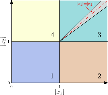
Figure 12: (color online) Different regions of the two-dimensional parameter space $|x_{1}|\times|x_{2}|$ in which the analytic expansions are performed. In region $3$, the silver area around the line $|x_{1}|=|x_{2}|$ indicates the region where the approximations lose precision, since the neglected terms of order $\mathcal{O}\left(\frac{1}{\left|x_{j}\right|}\left(\frac{\left|x_{<}\right|}{\left|x_{>}\right|}\right)^{2}\right)$, $j=1,2$, become more important.

In these expressions, both $y_{1}$ and $y_{2}$ can assume the values $\Omega_{0}=\Lambda$, $W_{1}=-\mu$, or $W_{2}=-\mu+\varepsilon_{0}$. To proceed with the calculation of (68) and (69), we use an asymptotic approach similar to that described in Appendix A. In each of the four regions of the two-dimensional parameter space $|x_{1}|\times|x_{2}|$ bounded by the lines $|x_{1}|=1$ and $|x_{2}|=1$ (see Fig.12), we substitute $\text{arctan}\left(\frac{|x_{i}|}{(2n+1)\pi}\right)$ and $\frac{|x_{i}|}{|x_{i}|^{2}+\left[(2n+1)\pi\right]^{2}}$ by their Taylor expansions in powers of $|x_{i}|$ if $|x_{i}|\ll 1$, or $1/|x_{i}|$ if $|x_{i}|\gg 1$.

When $|x_{i}|\gg 1$ we decompose the sums over $n$ into two contributions, $\sum\limits_{n=0}^{\infty}f(n)=\sum\limits_{n=0}^{N_{i}^{*}}f(n)+\sum\limits_{n=N_{i}^{*}+1}^{\infty}f(n)$, where $f(n)$ denotes any function of $n$. As in Appendix A, $N_{i}^{*}=\frac{|x_{i}|}{2\pi}-\frac{1}{2}$ is defined such that $(2N_{i}^{*}+1)\pi=|x_{i}|$. When both $|x_{1}|\gg 1$ and $|x_{2}|\gg 1$, the decomposition is such that $\sum\limits_{n=0}^{\infty}f(n)=\sum\limits_{n=0}^{N_{<}^{*}}f(n)+\sum\limits_{n=N_{<}^{*}+1}^{N_{>}^{*}}f(n)+\sum\limits_{n=N_{>}^{*}+1}^{\infty}f(n)$, with $N_{<}^{*}=\text{min}\{N_{1}^{*},N_{2}^{*}\}$ and $N_{>}^{*}=\text{max}\{N_{1}^{*},N_{2}^{*}\}$. Therefore, besides the sums already calculated in Eqs. (58), (63) and (64), we also need, for $\left|x_{i}\right|\gg 1$,

$$\sum\limits_{n=N_{1}^{*}}^{N_{2}^{*}}\frac{1}{\left[(2n+1)\pi\right]^{k}}\sim$$

$$\begin{cases}\frac{1}{2\pi}\ln\left(\frac{|x_{2}|}{|x_{1}|}\right)\text{,}&\text{ if }k=1\\[8.5359pt] \frac{1}{2\pi(k-1)}\left[\frac{1}{|x_{1}|^{k-1}}-\frac{1}{|x_{2}|^{k-1}}\right]\text{,}&\text{ if }k\leq 0\text{ or }k>1\end{cases}\text{,}$$ (70)

After a tedious but straightforward calculation, we then find the following asymptotic approximations for (68) and (69) in each of the four asymptotic regions of the $\left(\left|x_{1}\right|,\left|x_{2}\right|\right)$ plane:

$$s_{2}(\left|x_{1}\right|,\left|x_{2}\right|)\approx\begin{cases}0\text{ ,}&\text{ if }\left|x_{1}\right|,\,\left|x_{2}\right|\ll 1\\[8.5359pt] \kappa^{\prime}\left|x_{2}\right|\text{ ,}&\text{ if }\left|x_{1}\right|\gg 1\text{, }\left|x_{2}\right|\ll 1\\[8.5359pt] \frac{1}{2\left|x_{2}\right|}\ln\left(\kappa\left|x_{<}\right|\right)-\frac{\left|x_{1}\right|}{2\left|x_{>}\right|^{2}}+\frac{\left|x_{2}\right|\,\theta\left(\left|x_{1}\right|-\left|x_{2}\right|\right)}{4\left|x_{1}\right|^{2}}\text{ ,}&\text{ if }\left|x_{1}\right|,\,\left|x_{2}\right|\gg 1\\[8.5359pt] 0\text{ ,}&\text{ if }\left|x_{1}\right|\ll 1\text{, }\left|x_{2}\right|\gg 1\end{cases}$$ (71)

and

$$s_{3}(\left|x_{1}\right|,\left|x_{2}\right|)\approx\begin{cases}0\text{ ,}&\text{ if }\left|x_{1}\right|,\left|x_{2}\right|\ll 1\\[8.5359pt] \kappa^{\prime}\left|x_{2}\right|\text{ ,}&\text{ if }\left|x_{1}\right|\gg 1\text{, }\left|x_{2}\right|\ll 1\\[8.5359pt] \frac{\pi^{2}}{16}\!-\!\frac{(\left|x_{1}\right|+\left|x_{2}\right|)}{2\left|x_{1}\right|\left|x_{2}\right|}\!\ln\!\left(\kappa\left|x_{<}\right|\right)\!-\!\frac{1}{2\left|x_{<}\right|}+\frac{\left|x_{<}\right|}{2\left|x_{>}\right|^{2}}\text{ ,}&\text{ if }\left|x_{1}\right|,\left|x_{2}\right|\gg 1\\[8.5359pt] \kappa^{\prime}\left|x_{1}\right|\text{ ,}&\text{ if }\left|x_{1}\right|\ll 1\text{, }\left|x_{2}\right|\gg 1\end{cases}$$ (72)

Here, we defined the constant $\kappa^{\prime}=\frac{7\zeta(3)}{8\pi^{2}}\approx 0.11$ and defined $|x_{<}|=\text{min}\{|x_{1}|,|x_{2}|\}$ and $|x_{>}|=\text{max}\{|x_{1}|,|x_{2}|\}$. Recall that $\zeta(x)$ is the zeta function, $\theta\left(x\right)$ is the Heaviside step function and $\kappa\approx 1.13$ is the constant defined in Appendix A.

It is important to note that we treat the approximations we use during the derivation of Eqs.(71) and (72) consistently: in all the four regions of the parameter space shown in Fig.12, we kept only terms up to order $\mathcal{O}(\left|x\right|^{2})$, with $\left|x\right|\ll 1$. Note that there is a small sliver region around $|x_{1}|=|x_{2}|$ in region 3 where this approximation loses precision as compared to the other regions of the ($|x_{1}|$,$|x_{2}|$) plane.

The matrix elements of $\delta\hat{A}$, defined in Eq. (55), are given by combinations of (71) and (72). In each region of the phase diagram shown in Fig.3, the leading contributions yield for $R_{1}$:

$$R_{1}\sim\begin{cases}\frac{\Omega_{0}+\mu-\varepsilon_{0}}{2\Omega_{0}^{2}}+\frac{1}{2\Omega_{0}}\ln\left(\frac{\varepsilon_{0}-\mu}{\Omega_{0}}\right)\text{ ,}&\text{region I}\\[11.38092pt] \frac{4\Omega_{0}+\mu-2\varepsilon_{0}}{4\Omega_{0}^{2}}+\frac{\mu\;\theta\left(\varepsilon_{0}-2\mu\right)}{4\left(\varepsilon_{0}-\mu\right)^{2}}-\frac{\varepsilon_{0}-\mu}{2W_{>}^{2}}+\frac{1}{2\Omega_{0}}\ln\left(\frac{\varepsilon_{0}-\mu}{\Omega_{0}}\right)-\frac{1}{2\mu}\ln\left(\frac{\mu}{W_{<}}\right)\text{ ,}&\text{region II}\\[11.38092pt] \frac{4\Omega_{0}-\mu}{4\Omega_{0}^{2}}-\frac{1}{2\mu}\ln\left(\frac{\kappa\mu}{T_{c}}\right)+\frac{1}{2\Omega_{0}}\ln\left(\frac{\kappa\Omega_{0}}{T_{c}}\right)\text{ ,}&\text{region III}\\[11.38092pt] \frac{4\Omega_{0}+\mu-2\varepsilon_{0}}{4\Omega_{0}^{2}}+\frac{\mu-\varepsilon_{0}}{2\mu^{2}}-\frac{1}{2\mu}\ln\left(\frac{\kappa^{2}\mu\left(\mu-\varepsilon_{0}\right)}{T_{c}^{2}}\right)-\frac{1}{2\Omega_{0}}\ln\left(\frac{\kappa^{2}\Omega_{0}\left(\mu-\varepsilon_{0}\right)}{T_{c}^{2}}\right)\text{ ,}&\text{region IV}\\[11.38092pt] \end{cases}\text{ .}$$ (73)

For $R_{2}$, we find:

$$R_{2}\sim\begin{cases}\frac{\varepsilon_{0}-\mu}{4\Omega_{0}^{2}}+\frac{1}{2\left(\varepsilon_{0}-\mu\right)}\ln\left(\frac{\kappa\left(\varepsilon_{0}-\mu\right)}{T_{c}}\right)-\frac{1}{2\Omega_{0}}\ln\left(\frac{\kappa\Omega_{0}}{T_{c}}\right)\text{ ,}&\text{region I}\\[11.38092pt] \frac{\mu+\varepsilon_{0}}{4\Omega_{0}^{2}}-\frac{\mu}{2W_{>}^{2}}+\frac{\left(\varepsilon_{0}-\mu\right)\;\theta\left(2\mu-\varepsilon_{0}\right)}{4\mu^{2}}+\frac{1}{2\left(\varepsilon_{0}-\mu\right)}\ln\left(\frac{\kappa^{2}\left(\varepsilon_{0}-\mu\right)W_{<}}{T_{c}^{2}}\right)-\frac{1}{2\Omega_{0}}\ln\left(\frac{\kappa^{2}\mu\Omega_{0}}{T_{c}^{2}}\right)\text{ ,}&\text{region II}\\[11.38092pt] \frac{\Omega_{0}+\mu}{2\Omega_{0}^{2}}+\frac{2\kappa^{\prime}\left(\varepsilon_{0}-\mu\right)}{T_{c}^{2}}-\frac{1}{2\Omega_{0}}\ln\left(\frac{\kappa^{2}\mu\Omega_{0}}{T_{c}^{2}}\right)\text{ ,}&\text{region III}\\[11.38092pt] \frac{\mu+\varepsilon_{0}}{4\mu^{2}}+\frac{\mu+\varepsilon_{0}+4\Omega_{0}}{4\Omega_{0}^{2}}-\frac{1}{2\Omega_{0}}\ln\left(\frac{\kappa^{2}\Omega_{0}\mu}{T_{c}^{2}}\right)-\frac{1}{\mu-\varepsilon_{0}}\ln\left(\frac{\kappa\left(\mu-\varepsilon_{0}\right)}{T_{c}}\right)\text{ ,}&\text{region IV}\\[11.38092pt] \end{cases}\text{ ,}$$ (74)

and for $S$:

$$S\!\sim\!\begin{cases}\!\frac{1}{2\left(\varepsilon_{0}-\mu\right)}-\frac{\varepsilon_{0}-\mu}{2\Omega_{0}^{2}}+\frac{1}{2\left(\varepsilon_{0}-\mu\right)}\ln\left(\frac{\kappa\left(\varepsilon_{0}-\mu\right)}{T_{c}}\right)-\frac{1}{2\Omega_{0}}\ln\left(\frac{\kappa\Omega_{0}^{2}}{\left(\varepsilon_{0}-\mu\right)T_{c}}\right)\text{ ,}&\text{region I}\\[11.38092pt] \frac{2\mu-\varepsilon_{0}}{2\mu\left(\varepsilon_{0}-\mu\right)}\!-\!\frac{\varepsilon_{0}-2\mu}{2\Omega_{0}^{2}}+\!\frac{1}{2W_{<}}\!-\!\frac{W_{<}}{2W_{>}^{2}}\!+\frac{\varepsilon_{0}}{2\mu\left(\varepsilon_{0}-\mu\right)}\!\ln\!\left(\frac{\kappa W_{<}}{T_{c}}\right)\!-\!\frac{1}{2\mu}\!\ln\!\left(\frac{\kappa\mu}{T_{c}}\right)\!+\!\frac{1}{2\left(\varepsilon_{0}-\mu\right)}\!\ln\!\left(\frac{\kappa\left(\varepsilon_{0}-\mu\right)}{T_{c}}\right)\!-\!\frac{1}{2\Omega_{0}}\!\ln\!\left(\frac{\kappa^{2}\Omega^{2}\mu}{\left(\varepsilon_{0}-\mu\right)T_{c}^{2}}\right)\text{ ,}&\text{region II}\\[11.38092pt] \frac{\pi^{2}}{8T_{c}}-\frac{2\kappa^{\prime}\left(\varepsilon_{0}-\mu\right)}{T_{c}^{2}}-\frac{1}{2\mu}+\frac{\mu}{2\Omega_{0}^{2}}-\frac{1}{2\mu}\ln\left(\frac{\kappa\mu}{T_{c}}\right)-\frac{1}{2\Omega_{0}}\ln\left(\frac{\kappa^{3}\Omega_{0}^{2}\mu}{T_{c}^{3}}\right)\text{ ,}&\text{region III}\\[11.38092pt] \frac{\pi^{2}}{4T_{c}}-\frac{1}{\mu-\varepsilon_{0}}-\frac{\varepsilon_{0}}{2\mu^{2}}+\frac{2\mu-\varepsilon_{0}}{2\Omega_{0}^{2}}-\frac{1}{2\Omega_{0}}\ln\left(\frac{\kappa^{4}\Omega_{0}^{2}\mu\left(\mu-\varepsilon_{0}\right)}{T_{c}^{4}}\right)-\frac{1}{2\mu}\ln\left(\frac{\kappa^{2}\mu\left(\mu-\varepsilon_{0}\right)}{T_{c}^{2}}\right)-\frac{1}{\mu-\varepsilon_{0}}\ln\left(\frac{\kappa\left(\mu-\varepsilon_{0}\right)}{T_{c}}\right)\text{ ,}&\text{region IV}\\[11.38092pt] \end{cases}\text{ ,}$$ (75)

where, $W_{<}\equiv\text{min}\{|W_{1}|,|W_{2}|\}$ and $W_{>}\equiv\text{max}\{|W_{1}|,|W_{2}|\}$. The order of the terms in the expressions for $R_{1}$, $R_{2}$ and $S$ are also consistent with those in Eqs.(71) and (72).

Appendix C $T_{c}(\mu)$ and $\partial T_{c}/\partial\tau_{ij}^{-1}$ in the dilute regime

Here, we provide more details about the calculation of the analytic asymptotic expression of $T_{c}$, as well as its suppression rate by inter-band non-magnetic impurity scattering, $\left.\frac{\partial T_{c}}{\partial\tau_{\mathrm{inter}}^{-1}}\right|_{\tau_{\mathrm{inter}}^{-1}=0}$, as function of the chemical potential.

Recalling that we denote by $\alpha(T)$ the largest eigenvalue of $\hat{\lambda}\hat{A}_{d}$, where $\hat{A}_{d}$ is defined in Eq.(53), it follows that, similarly to Sec.II.2, finding $T_{c}(\mu)$ involves solving a transcendental algebraic equation $\alpha=1$, with:

$$\alpha=\frac{1}{2}\left[a_{11}+a_{22}+\sqrt{(a_{11}-a_{22})^{2}+4a_{12}a_{21}}\right]\text{,}$$ (76)

where we defined, in terms of the analytic expressions for $R_{i}$ and $S$ calculated in Appendix B:

$$a_{11} =\lambda_{11}\left[A_{1}+\frac{\tau_{\mathrm{inter}}^{-1}}{2\pi}\left(R_{1}-S\right)\right]+\frac{\tau_{\mathrm{inter}}^{-1}}{2\pi}\lambda_{12}S$$

$$a_{12} =\lambda_{12}\left[A_{2}+\frac{\tau_{\mathrm{inter}}^{-1}}{2\pi}\left(R_{2}-S\right)\right]+\frac{\tau_{\mathrm{inter}}^{-1}}{2\pi}\lambda_{11}S$$

$$a_{21} =\lambda_{12}\left[A_{1}+\frac{\tau_{\mathrm{inter}}^{-1}}{2\pi}\left(R_{1}-S\right)\right]+\frac{\tau_{\mathrm{inter}}^{-1}}{2\pi}\lambda_{22}S$$

$$a_{22} =\lambda_{22}\left[A_{2}+\frac{\tau_{\mathrm{inter}}^{-1}}{2\pi}\left(R_{2}-S\right)\right]+\frac{\tau_{\mathrm{inter}}^{-1}}{2\pi}\lambda_{12}S\text{ ,}$$ (77)

with $A_{1}=\left(\hat{A}_{c}\right)_{11}$ and $A_{2}=\left(\hat{A}_{c}\right)_{22}$. The resulting $T_{c}(\mu)$, for both attractive ($\lambda_{12}>0$) and repulsive ($\lambda_{12}<0$) inter-band superconducting interaction, and its comparison with the numeric solution of the gap equations are shown in Fig. 8.

Once we know $T_{c}(\mu)$, it is straightforward to compute $\frac{\partial T_{c}}{\partial\tau_{\mathrm{inter}}^{-1}}$ from Eq.(31). It follows that the different terms entering Eq.(31), also in terms of the analytical expressions for $R_{i}$ and $S$, are given by:

$$\left\langle\alpha_{L}^{(0)}\left|\frac{\partial(\hat{\lambda}\hat{A}_{d})}{\partial\tau_{\mathrm{inter}}^{-1}}\right|\alpha_{R}^{(0)}\right\rangle=\frac{1}{2\pi} \left\{(1-\lambda_{11}A_{2})\left[(R_{1}-S)(\lambda_{11}-\lambda_{11}^{2}A_{2}+\lambda_{12}^{2}A_{2})+\lambda_{12}S(1+\lambda_{11}A_{1})\right]\right.$$

$$\left.+\lambda_{12}^{2}A_{1}(R_{2}-S+\lambda_{12}SA_{2})\right\}\text{ ,}$$ (78)

and

$$\left.\frac{\partial\alpha_{0}}{\partial T}\right|_{T=T_{c}}=\frac{1}{2-\lambda_{11}(A_{1}+A_{2})}\sum\limits_{j=1}^{2}\left(\lambda_{11}-\lambda_{11}^{2}A_{j}+\lambda_{12}^{2}A_{j}\right)\left.\frac{\partial A_{\bar{j}}}{\partial T}\right|_{T=T_{c}}$$ (79)

as well as

$$\left\langle\left.\alpha_{L}^{(0)}\right|\alpha_{R}^{(0)}\right\rangle=(1-\lambda_{11}A_{2})^{2}+\lambda_{12}^{2}A_{1}A_{2}\text{ .}$$ (80)

In the previous equations, $A_{i}\equiv\left(\hat{A}_{c}\right)_{ii}$ and we set $\lambda_{11}=\lambda_{22}$ for simplicity. The resulting $\left.\frac{\partial T_{c}}{\partial\tau_{\mathrm{inter}}^{-1}}\right|_{\tau_{\mathrm{inter}}^{-1}=0}$, for both attractive and repulsive inter-band superconducting interaction, are shown in Fig. 9.

References

- (1) H. Suhl, T. B. Matthias and R. L. Walker, Phys. Rev. Lett., 3, 552 (1959).
- (2) V. A. Moskalenko, Fiz. Met. Mettaloved. 8, 503 (1959).
- (3) A. Y. Liu, I. I. Mazin, and J. Kortus, Phys. Rev. Lett. 87, 087005 (2001).
- (4) M. Marz, G. Goll, W. Goldacker, and R. Lortz, Phys. Rev. B 82, 024507 (2010).
- (5) T. Yokoya, T. Kiss, A. Chainani, S. Shin, M. Nohara, and H. Takagi, Science 294, 2518 (2001).
- (6) H. Ding, P. Richard, K. Nakayama, K. Sugawara, T. Arakane, Y. Sekiba, A. Takayama, S. Souma, T. Sato, T. Takahashi, Z. Wang, X. Dai, Z. Fang, G. F. Chen, J. L. Luo, and N. L.Wang, EPL 83, 47001 (2008).
- (7) A. P. Mackenzie, S. R. Julian, A. J. Diver, G. J. McMullan, M. P. Ray, G. G. Lonzarich, Y. Maeno, S. Nishizaki, and T. Fujita, Phys. Rev. Lett. 76, 3786 (1996).
- (8) P. M. C. Rourke, M. A. Tanatar, C. S. Turel, J. Berdeklis, C. Petrovic, and J. Y. T. Wei, Phys. Rev. Lett. 94, 107005 (2005).
- (9) X. Lin, G. Bridoux, A. Gourgout, G. Seyfarth, S. Krämer, M. Nardone, B. Fauqué, and K. Behnia, Phys. Rev. Lett. 112, 207002 (2014).
- (10) G. Binnig, A. Baratoff, H. E. Hoenig, and J. G. Bednorz, Phys. Rev. Lett. 45, 1352 (1980).
- (11) A. Joshua, S. Pecker, J. Ruhman, E. Altman, and S. Ilani, Nat. Commun. 3, 1129 (2012).
- (12) S. E. Rowley, L. J. Spalek, R. P. Smith, M. P. M. Dean, M. Itoh, J. F. Scott, G. G. Lonzarich, and S. S. Saxena, Nat. Phys. 10, 367 (2014).
- (13) J. M. Edge, Y. Kedem, U. Aschauer, N. A. Spaldin, and A. V. Balatsky, Phys. Rev. Lett. 115, 247002 (2015).
- (14) L. P. Gor’kov, arXiv:1610.02062.
- (15) J. Ruhman and P. A. Lee, Phys. Rev. B 94, 224515 (2016).
- (16) J. R. Arce-Gamboa, G. G. Guzmán-Verri, arXiv:1801.08736.
- (17) M. S. Scheurer and J. Schmalian, Nat. Comm. 6, 6005 (2015).
- (18) D. V. Efremov, M. M. Korshunov, O. V. Dolgov, A. A. Golubov, and P. J. Hirschfeld, Phys. Rev. B 84, 180512(R) (2011).
- (19) S. Maiti and A. V. Chubukov, Phys. Rev. B 87, 144511 (2013).
- (20) E. Babaev and M. Speight, Phys. Rev. B 72, 180502(R) (2005).
- (21) J. Geyer, R. M. Fernandes, V. G. Kogan, and J. Schmalian, Phys. Rev. B 82, 104521 (2010).
- (22) L. Komendova, Y. Chen, A. A. Shanenko, M. V. Milosevic, and F. M. Peeters, Phys. Rev. Lett. 108, 207002 (2012).
- (23) L. Komendova, A. V. Balatsky, and A. M. Black-Schaffer, Phys. Rev. B 92, 094517 (2015).
- (24) M. Silaev and E. Babaev, Phys. Rev. B 84, 094515 (2011).
- (25) I. M. Lifshitz, Sov. Phys. JETP 11, 1130 (1960).
- (26) A. Bianconi, Sol. State Commun. 89, 933 (1994).
- (27) R. M. Fernandes, J. T. Haraldsen, P. Wölfle, and A. V. Balatsky, Phys. Rev. B 87, 014510 (2013).
- (28) A. Bianconi, D. Innocenti, A. Valletta and A. Perali, J. Phys.: Conf. Ser. 529, 012007 (2014).
- (29) A. V. Chubukov, I. Eremin, and D. V. Efremov, Phys. Rev. B 93, 174516 (2016).
- (30) J. M. Edge and A. V. Balatsky, J. Supercond. Nov. Magn. 28, 2373 (2015).
- (31) X. Chen, V. Mishra, S. Maiti, and P. J. Hirschfeld, Phys. Rev. B 94, 054524 (2016).
- (32) Y. Bang, New J. Phys. 16, 023029 (2014).
- (33) X. Chen, S. Maiti, A. Linscheid, and P. J. Hirschfeld, Phys. Rev. B 92, 224514 (2015).
- (34) D. Innocenti, N. Poccia, A. Ricci, A. Valletta, S. Caprara, A. Perali, and A. Bianconi, Phys. Rev. B 82, 184528 (2010).
- (35) K. W. Song and A. E. Koshelev, Phys. Rev. B 95, 174503 (2017).
- (36) D. Valentinis, D. van der Marel, and C. Berthod, Phys. Rev. B 94, 024511 (2016).
- (37) C. Liu, A. D. Palczewski, R. S. Dhaka, T. Kondo, R. M. Fernandes, E. D. Mun, H. Hodovanets, A. N. Thaler, J. Schmalian, S. L. Bud’ko, P. C. Canfield, and A. Kaminski, Phys. Rev. B 84, 020509(R) (2011).
- (38) Y. Nakajima, R. Wang, T. Metz, X. Wang, L. Wang, H. Cynn, S. T. Weir, J. R. Jeffries, and J. Paglione, Phys. Rev. B 91, 060508(R) (2015).
- (39) T. V. Trevisan, M. Schütt, R. M. Fernandes, Phys. Rev. Lett. 121, 127002 (2018).
- (40) D. J. Bergmann and D. Rainer, Z. Phys. 263, 59 (1973).
- (41) J. Kang and R. M. Fernandes, Phys. Rev. B 93, 224514 (2016).
- (42) A. A. Golubov and I. I. Mazin, Phys. Rev. B 55, 15146 (1997).
- (43) Y. Wang, A. Kreisel, P. J. Hirschfeld, and V. Mishra, Phys. Rev. B 87, 094504 (2013).
- (44) M. S. Scheurer, M. Hoyer and J. Schmalian, Phys. Rev. B 92 014518 (2015).