Abstract

In this paper we introduce a new gradient method which attains quadratic convergence in a certain sense. Applicable to infinite-dimensional unconstrained minimization problems posed in a Hilbert space $H$, the approach consists in finding the energy gradient $g(\lambda)$ defined with respect to an optimal inner product selected from an infinite family of equivalent inner products $(\cdot,\cdot)_{\lambda}$ in the space $H$. The inner products are parameterized by a space-dependent weight function $\lambda$. At each iteration of the method, where an approximation to the minimizer is given by an element $u\in H$, an optimal weight ${\widehat{\lambda}}$ is found as a solution of a nonlinear minimization problem in the space of weights $\Lambda$. It turns out that the projection of $\kappa g({\widehat{\lambda}})$, where $0<\kappa\ll 1$ is a fixed step size, onto a certain finite-dimensional subspace generated by the method is consistent with Newton’s step $h$, in the sense that $P_{u}(\kappa g({\widehat{\lambda}}))=P_{u}(h)$, where $P_{u}$ is an operator describing the projection onto the subspace. As demonstrated by rigorous analysis, this property ensures that thus constructed gradient method attains quadratic convergence for error components contained in these subspaces, in addition to the linear convergence typical of the standard gradient method. We propose a numerical implementation of this new approach and analyze its complexity. Computational results obtained based on a simple model problem confirm the theoretically established convergence properties, demonstrating that the proposed approach performs much better than the standard steepest-descent method based on Sobolev gradients. The presented results offer an explanation of a number of earlier empirical observations concerning the convergence of Sobolev-gradient methods.

Keywords: unconstrained optimization in Hilbert spaces, variable inner products, Sobolev gradients, Newton’s method, gradient method with quadratic convergence
MSC (2010): primary 49M05, 49M15, 97N40; secondary 65K10, 78M50

1 Introduction

In this investigation we consider solution of general unconstrained optimization problems using the steepest-descent method and focus on modifying the definition of the gradient such that in certain circumstances this approach will achieve a quadratic convergence, characteristic of Newton’s method. This is accomplished by judiciously exploiting the freedom inherent in the choice of different equivalent norms defining the gradient through the Riesz representation theorem. This freedom can be used to adjust the definition of the inner product, such that the resulting gradient will, in a suitable sense, best resemble the corresponding Newton step. While such ideas can be pursued in both finite-dimensional and infinite-dimensional settings, the formulation is arguably more interesting mathematically and more useful in practice in the latter case. We will thus consider unconstrained optimization problems of the general form

$$e({\widehat{u}})=\min\{e(u),\;u\in H\},$$ (1)

where $e\;:\;H\mapsto\mathbb{R}$ is the objective functional and $H$ is a suitable function space with Hilbert structure. Applications which have this form include, for example, minimization of various energy functionals in physics and optimization formulations of inverse problems, where evaluation of the objective functional $e(u)$ may involve solution of a complicated (time-)dependent partial differential equation (PDE). In such applications $H$ is typically taken as a Sobolev space $H^{p}(\Omega)$, $p\in\mathbb{N}$, where $\Omega\subset\mathbb{R}^{d}$ is the spatial domain assumed to be sufficiently smooth (Lipschitz) and $d\geq 1$ is the dimension [1]. Therefore, to fix attention, here we will assume $H:=H^{1}_{0}(\Omega)$ with the inner product and norm in $H$ defined as

$$(u,v)_{H}=\int_{\Omega}((\nabla u\cdot\nabla v)+uv)\,dx,\qquad\|u\|_{H}=(u,v)_{H}^{1/2}.$$ (2)

1:  set $u=u_{0}$

2:  repeat

3:     compute $e^{\prime}(u;\cdot)$

4:     determine $g\in H$ as the solution of $(g,v)_{H}=e^{\prime}(u;v)$, $\forall v\in H$

5:     set $\widetilde{u}=u-\kappa g$

6:     set $u=\widetilde{u}$

7:  until    $|e(u)|<$ err

Algorithm 1 (Sobolev) Gradient method
Input:
      $u_{0}\in H$ — initial guess
      $\kappa>0$ — step size (sufficiently small)
      $\texttt{err}>0$ — tolerance
Output:
      $\widetilde{u}$ — approximation to the solution ${\widehat{u}}$ of problem (1)

1:  set $u=u_{0}$

2:  repeat

3:     compute $e^{\prime}(u;\cdot)$

4:     compute $e^{\prime\prime}(u;\cdot,\cdot)$

5:     determine $h\in H$ as the solution of $e^{\prime\prime}(u;h,v)=e^{\prime}(u;v)$, $\forall v\in H$

6:     set $\widetilde{u}=u-h$

7:     set $u=\widetilde{u}$

8:  until    $|e(u)|<$ err

Algorithm 2 Newton’s method
Input:
      $u_{0}\in H$ — initial guess
      $\texttt{err}>0$ — tolerance
Output:
      $\widetilde{u}$ — approximation to the solution ${\widehat{u}}$ of problem (1)

The two most elementary approaches to solve problem (1) are the gradient and Newton’s method which, for the sake of completeness, are defined in Algorithms 1 and 2, respectively. The former approach is sometimes also referred to as the “Sobolev gradient” method [10]. While gradient approaches often involve an adaptive step size selection [11], for simplicity of analysis in Algorithm 1 we consider a fixed step size $\kappa=\text{Const}$. Likewise, in order to keep the analysis tractable, we do not consider common modifications of the gradient approach such as the conjugate-gradient method. As regards convergence of the gradient and Newton’s method, we have the following classical results, see for example [5].

Theorem 1.1

Let ${\widehat{u}}\in H$ be a solution of (1). Assume that $e$ is twice differentiable near ${\widehat{u}}$ and there exist $\delta_{0}>0$ and $\alpha_{0}>0$ such that $e^{\prime\prime}(u;v,v)\geq\alpha_{0}\|v\|^{2}_{H}$ for all $\|u-{\widehat{u}}\|_{H}\leq\delta_{0}$ and $v\in H$. Then, for all $u_{0}\in B_{H}({\widehat{u}},\delta_{0})$ the gradient method given by Algorithm 1 converges linearly to ${\widehat{u}}$ in $H$, i.e.,

$$\|\widetilde{u}-{\widehat{u}}\|_{H} \leq \epsilon\|u-{\widehat{u}}\|_{H},$$

with $\epsilon\in(0,1)$ depending only on $e$ and $\kappa$.

Theorem 1.2

Let ${\widehat{u}}\in H$ be a solution of (1). Assume that $e$ is three times differentiable near ${\widehat{u}}$ and that the map $v\in H\mapsto e^{\prime\prime}({\widehat{u}};v,\cdot)\in H^{\prime}$ is invertible. Then, there exists $\delta_{0}>0$ such that for all $u_{0}\in B_{H}({\widehat{u}},\delta_{0})$ Newton’s method given by Algorithm 2 converges quadratically to ${\widehat{u}}$ in $H$, i.e.,

$$\|\widetilde{u}-{\widehat{u}}\|_{H} \leq C\|u-{\widehat{u}}\|^{2}_{H},$$

with $C>0$ depending only on $e$.

We emphasize that in Algorithm 1 the gradient $g$ must be computed with respect to the topology of the space $H$ in which the solution to (1) is sought [10], an aspect of the problem often neglected in numerical investigations. A metric equivalent to $\|\cdot\|_{H}$ (in the precise sense of norm equivalence) can be obtained by redefining the inner product in (2) more generally as follows

$$(u,v)_{\lambda_{0}}=\int_{\Omega}(\lambda_{0}(\nabla u\cdot\nabla v)+uv)\,dx,$$ (3)

where $\lambda_{0}\in(0,\infty)$ is a fixed constant. While as compared to (2) definition (3) does not change the analytic structure of the optimization problem (1), there is abundant computational evidence obtained in the solution of complicated optimization problems [13, 14, 2] that convergence of gradient Algorithm 1 may be significantly accelerated by replacing the inner product from (2) with the one introduced in (3) for some judicious choices of the parameter $\lambda_{0}$. Likewise, a similar acceleration was also observed when the inner product in (2) was replaced with another equivalent definition motivated by the structure of the minimization problem and different from (3), cf. [16, 12, 8]. In the absence of an understanding of the mechanism responsible for this acceleration, the parameter $\lambda_{0}$, or other quantities parameterizing the equivalent inner product, were chosen empirically by trial and error, which is unsatisfactory.

In the present investigation we will consider a more general form of the inner product (3) in which the constant $\lambda_{0}$ is replaced with a space-dependent weight $\lambda=\lambda(x)$. Our goal is to develop a rational and systematic approach allowing one to accelerate the convergence of gradient iterations in Algorithm 1 in comparison to the standard case by adaptively adjusting the weight $\lambda(x)$. This will result in a reduction of the total number of iterations needed to solve problem (1) to a given accuracy, but each iteration will be more costly.

Modifications of the inner product with respect to which the gradient is defined may also be interpreted as gradient preconditioning and this perspective is pursued in the monograph [17] focused on related problems arising in the solution of nonlinear elliptic equations. The relationship between the gradient and Newton’s methods was explored in [18] where a variable inner product was considered. In contrast to the present approach in which the inner-product weights are sought by matching the projections of the gradient and Newton’s steps onto a certain subspace, in [18] optimal inner products were found by maximizing the descent achieved at a given iteration with respect to the structure of the corresponding preconditioning operator.

The structure of the paper is as follows. In the next section we define the new approach in a general form, whereas in Section 3 we prove its convergence properties. Then, in Section 4 we describe the numerical approach implementing the general method introduced in Section 2 in two variants and analyze its computational complexity. Our model problem and computational results are presented in Section 5, whereas discussion and conclusions are deferred to Section 6.

2 A new gradient method based on an optimal inner product

In this section we introduce our modified version of Algorithm 1 for the solution of the minimization problem (1). We begin by making the following assumptions on the energy $e(u)$:

$$e \mbox{\it is $C^{2}$ in $H$},$$ (4)

$$|e^{\prime\prime}(u;v,w)| \leq M\|u\|_{H}\|w\|_{H},\quad u,v,w\in H,$$ (5)

$$e^{\prime\prime}(u;v,v) \geq m\|v\|_{H}^{2},$$ (6)

with certain $M,m>0$.

Let us point out that at each step of both the gradient and Newton’s methods the descent direction is defined by the solution of the equation

$$b(z,v)=e^{\prime}(u;v),\quad\forall v\in H,$$ (7)

where $b(u,v)$, a symmetric bilinear continuous elliptic form, and $z\in H$ are specific to each method, namely,

• $b(u,v)=(u,v)_{H}$ and $z=g$ in the case of the gradient method, and

• $b(u,v)=e^{\prime\prime}(u;u,v)$ and $z=h$ in the case of Newton’s method.

Moreover, we note that the solution $z$ of (7) is also the solution of the minimization problem

$$\min\left\{\frac{1}{2}b(v,v)-e^{\prime}(u;v),\;\,v\in H\right\}.$$ (8)

We emphasize that, in fact, Newton’s method may be also viewed as a “gradient” method with a particular choice of the inner product at each iteration, namely, the one induced by $e^{\prime\prime}(u)$. Therefore, the idea for improving the classical gradient method is to make the gradient step $g$ “close” to the Newton step $h$ by suitably adapting the inner product in $H$.

We thus propose the following modification of the gradient method from Algorithm 1. We want to consider the gradient $g$ defined with respect to an inner product in $H$ depending on a function parameter $\lambda$. Typically, $0<\lambda\in C^{0}(\overline{\Omega})$, however, to make our method more attractive from the computational point of view we will consider $\lambda$ with a finite range. Namely, let $\{\Omega_{i},\,i=1,\ldots,N\}$, be a partition of $\Omega$ into open Lipschitz sets, $\Lambda=\{\lambda:\Omega\mapsto\mathbb{R},\,\;\lambda(\Omega_{i})=\lambda_{i}\in\mathbb{R}\}=\operatorname{span}\{\ell^{i},\,i=1,\dots,N\}\subset L^{\infty}(\Omega)$, where $\ell^{i}\in\Lambda$, $\ell^{i}=\delta_{i,j}$ in $\Omega_{j}$, $i,j=1,\ldots,N$ with $\delta_{i,j}$ the Kronecker symbol, $\Lambda^{+}=\Lambda\cap\{0<\lambda<\infty\}$. Sometimes without the risk of confusion we will write $\lambda=[\lambda_{1},\ldots,\lambda_{N}]\in\mathbb{R}^{N}$ for $\lambda\in\Lambda$, meaning $\lambda(\Omega_{i})=\lambda_{i}$, for all $i=1,\ldots,N$. Then, for $\lambda\in\Lambda^{+}$, we define the following inner product and norm in $H$

$$(v,w)_{\lambda}=\int_{\Omega}\lambda(\nabla v\cdot\nabla w)+vw\,dx,\quad\|v\|_{\lambda}=(v,v)_{\lambda}^{1/2},\quad\forall v,w\in H.$$ (9)

Clearly, $(\cdot,\cdot)_{\lambda}$ and $(\cdot,\cdot)_{H}=(\cdot,\cdot)_{1}$ are equivalent in $H$ and therefore we can use $(\cdot,\cdot)_{\lambda}$ instead of $(\cdot,\cdot)_{H}$ for the gradient method.

The idea is to use the inner product $(\cdot,\cdot)_{\lambda}$ in the gradient method, with $\lambda$ judiciously chosen. More specifically, for $\lambda\in\Lambda^{+}$, let $g=g(\lambda)$ be the solution of

$$(g,v)_{\lambda}=\int_{\Omega}\lambda(\nabla{g}\cdot\nabla v)+{g}v\,dx=e^{\prime}(u;v),\quad\forall v\in H.$$ (10)

Remark 2.1

In the following we will, in particular, refer to the gradient $g_{1}:=g(1)$ which corresponds to the usual inner product (2) and is also obtained by setting $\lambda=1$ in (10), and to the gradient $g_{0}:=g(0)$ which corresponds to $\lambda=0$ in (10). Usually, $g_{1}$ and $g_{0}$ are referred to as, respectively, the $H^{1}$ and $L^{2}$ Riesz representations of $e^{\prime}(u)$.

In general $g_{0}\notin H^{1}_{0}(\Omega)$, but we have

$$-\Delta g_{1}+g_{1} = g_{0}\;\,\mbox{\it in ${\cal D^{\prime}}(\Omega)$},$$ (11)

$$-\nabla\cdot(\lambda\nabla g(\lambda))+g(\lambda) = g_{0}\;\,\mbox{\it in ${\cal D^{\prime}}(\Omega)$}.$$ (12)

Note that we will use the symbol $g$ to denote the operator $\lambda\in\Lambda\mapsto g=g(\lambda)\in H$, or to denote an element of $H$ — the meaning will always be clear from the context.

Now assume we are at a certain iteration of the gradient method with $u$ known, which we seek to update to a new value $\widetilde{u}$, cf. step 5 in Algorithm 1. For this, first we look for a certain ${\widehat{\lambda}}\in\Lambda^{+}$, defined by

$$j({\widehat{\lambda}}):=\min\left\{j(\lambda):=f\circ g(\lambda),\;\,\lambda\in\Lambda^{+}\right\},\quad\text{\it where}\quad f(g):=\frac{\kappa}{2}e^{\prime\prime}(u;g,g)-e^{\prime}(u;g).$$ (13)

The reason for introducing the step size $\kappa$ in this equality will be clear from Remark 2.2 and also later during the error analysis in Section 3. Note that, if problem (13) has a solution ${\widehat{\lambda}}\in\Lambda^{+}$, then we will show (see Proposition 3.1) that ${\widehat{\lambda}}$ solves

$$e^{\prime\prime}(u;\kappa g({\widehat{\lambda}}),g^{\prime}({\widehat{\lambda}};\ell))=e^{\prime}(u;g^{\prime}({\widehat{\lambda}};\ell)),\quad\forall\ell\in\Lambda,$$ (14)

where $g^{\prime}({\widehat{\lambda}};\ell)$ denotes the derivative of $g$ at ${\widehat{\lambda}}$ in the direction $\ell$. Then, the modified gradient approach will consist of Algorithm 1 with step 4 amended as follows

$$4. \mbox{determine $g=g({\widehat{\lambda}})$, where ${\widehat{\lambda}}\in\Lambda^{+}$ is such that $g({\widehat{\lambda}})\in H$ solves (\ref{e:e''(lambda)=e'})}.$$ (15)

Remark 2.2

Clearly, our approach is equivalent to the gradient method, but with the classical inner product $(\cdot,\cdot)_{H}$ replaced with $(\cdot,\cdot)_{\lambda}$.

From equation (14) it follows that $e^{\prime\prime}(u;h-\kappa g,g^{\prime}({\widehat{\lambda}};\ell))=0$, where $h$ is Newton’s step. This means that $P_{u}(h-\kappa g)=0$, where $P_{u}:H\mapsto T_{u}$ is the projection from $H$ to $T_{u}$, in which $T_{u}=\operatorname{span}\{g^{\prime}({\widehat{\lambda}};\ell),\;\ell\in\Lambda\}$ is the tangent space to the manifold $\{g(\lambda),\,\lambda\in\Lambda^{+}\}\subset H$ at $g({\widehat{\lambda}})$, determined with respect to the inner product $e^{\prime\prime}(u;\cdot,\cdot)$.

If $T_{u}=H$, then $\kappa g({\widehat{\lambda}})=h$ and our method reduces to Newton’s method. However, here we have $dim(\Lambda)=N$, so that in general $T_{u}\neq H$ and $\kappa g$ will be close to $h$ in the sense that $P_{u}(h-\kappa g)=0$. This relation will be the key ingredient to prove in the demonstration that our gradient method, in addition to the linear convergence of a standard gradient method, has also a quadratic convergence in a certain sense depending on $T_{u}$ and the projection $P_{u}$. This will be explained in the next sections.

Our method critically depends on the choice of $\lambda$ and the following proposition offers a first glimpse of what may happen with the solution of problem (13).

Proposition 2.3

Let $(\lambda^{k})$ be a minimizing sequence of $j$ in $\Lambda^{+}$ and $(g(\lambda^{k}))$ be the corresponding sequence of gradients defined in (10). Then, up to a subsequence, $(g(\lambda^{k}))$ converges weakly in $H^{1}_{0}(\Omega)$ and strongly in $L^{2}(\Omega)$ to an element $g\in H$, while for the sequence $(\lambda^{k})$ one of the following cases may occur.
(i) There exist ${\widehat{\lambda}}=[{\widehat{\lambda}}_{1},\ldots,{\widehat{\lambda}}_{N}]\in\Lambda^{+}$ and a subsequence of $(\lambda^{k})$, still denoted $(\lambda^{k})$, such that $\lim_{k\to\infty}\lambda^{k}_{i}={\widehat{\lambda}}_{i}$ for all $i=1,\dots,N$. In this case $g=g({\widehat{\lambda}})$, i.e.

$$\int_{\Omega}{\widehat{\lambda}}(\nabla g({\widehat{\lambda}})\cdot\nabla v)+g({\widehat{\lambda}})v\,dx=e^{\prime}(u;v),\;\,\forall v\in H,$$ (16)

and ${\widehat{\lambda}}$ solves (13).
(ii) There exist ${\widehat{\lambda}}=[{\widehat{\lambda}}_{1},\ldots,{\widehat{\lambda}}_{N}]\in\partial\Lambda^{+}$, $I_{0}\subset I$, $I_{\infty}\subset I$, with ${\widehat{\lambda}}_{i}=0$ for all $i\in I_{0}$, ${\widehat{\lambda}}_{i}=+\infty$ for all $i\in I_{\infty}$, $0<{\widehat{\lambda}}_{i}<+\infty$ for all $i\in I\backslash(I_{0}\cup I_{\infty})$, and a subsequence of $(\lambda^{k})$, still denoted $(\lambda^{k})$, such that $\lim_{k\to\infty}\lambda^{k}_{i}={\widehat{\lambda}}_{i}$, for all $i=1,\dots,N$. In this case $g\in H^{1}_{0}(\Omega;\Omega_{\infty}^{\text{const}})$ solves

$$\int_{\Omega\backslash\Omega_{0}}{\widehat{\lambda}}(\nabla g\cdot\nabla v)+gv\,dx+\int_{\Omega_{0}}gv\,dx = e^{\prime}(u;v),\quad\forall v\in H^{1}_{0}(\Omega;\Omega_{\infty}^{\text{const}}),$$ (17)

where

$$\Omega_{0} = \cup\{\Omega_{i},\;i\in I_{0}\},$$ (18)

$$\Omega_{\infty} = \cup\{\Omega_{i},\;i\in I_{\infty}\},$$ (19)

$$H^{1}_{0}(\Omega;\Omega_{\infty}^{\text{const}}) = \{v\in H^{1}_{0}(\Omega),\;\,v=C_{i}\in\mathbb{R}\;\,in\;\,\Omega_{i},\;\,\forall i\in I_{\infty}\}.$$ (20)

Furthermore, if we define $g({\widehat{\lambda}})=g$, with $g$ given by (17), we have

$$j({\widehat{\lambda}})\leq\liminf_{k\to\infty}j(\lambda^{k}).$$ (21)

Proof. Let $(\lambda^{k})$ be a minimizing sequence of $j$ in $\Lambda^{+}$ and $\lambda^{k}=[\lambda^{k}_{1},\ldots,\lambda^{k}_{N}]$. Note that $g(\lambda^{k})$ is well defined by

$$\int_{\Omega}\lambda^{k}(\nabla g(\lambda^{k})\cdot\nabla v)+g(\lambda^{k})v\,dx=e^{\prime}(u;v),\quad\forall v\in H.$$ (22)

Note also that from the ellipticity of $f$ in $H$, cf. (5), (6) and (13), it follows that the sequence $g(\lambda^{k})$ is bounded in $H^{1}(\Omega)$. Therefore, up to a subsequence, we may assume that $g(\lambda^{k})$ converges weakly in $H$ and strongly in $L^{2}(\Omega)$ to a certain $g\in H$.

As ${\rm dim}(\Lambda)=N$, there exist ${\widehat{\lambda}}=[{\widehat{\lambda}}_{1},\ldots,{\widehat{\lambda}}_{\color[rgb]{0,0,0}N}]$, with ${\widehat{\lambda}}_{i}\in[0,+\infty]$, and a subsequence of $(\lambda^{k})$, still denoted $(\lambda^{k})$, such that $\lim_{k\to\infty}\lambda^{k}_{i}={\widehat{\lambda}}_{i}$ for all $i\in I$. Two cases may occur.
1) ${\widehat{\lambda}}\in\Lambda^{+}$, i.e., ${\widehat{\lambda}}_{i}\in(0,\infty)$ for all $i\in I$. From (22) we obtain

$$\int_{\Omega}{\widehat{\lambda}}(\nabla g\cdot\nabla v)+gv\,dx = \int_{\Omega}({\widehat{\lambda}}-\lambda^{k})(\nabla g\cdot\nabla v)\,dx$$

$$+ \int_{\Omega}\lambda^{k}(\nabla(g-g(\lambda^{k}))\cdot\nabla v)+(g-g(\lambda^{k}))v\,dx$$

$$+ \int_{\Omega}\lambda^{k}(\nabla g(\lambda^{k})\cdot\nabla v)+g(\lambda^{k})v\,dx$$

$$= \int_{\Omega}({\widehat{\lambda}}-\lambda^{k})(\nabla g\cdot\nabla v)\,dx$$

$$+ \int_{\Omega}\lambda^{k}(\nabla(g-g(\lambda^{k}))\cdot\nabla v)+(g-g(\lambda^{k}))v\,dx$$

$$+ e^{\prime}(u;v),\quad\forall v\in H.$$

Then, letting $k$ go to infinity gives

$$\int_{\Omega}{\widehat{\lambda}}(\nabla g\cdot\nabla v)+gv\,dx = e^{\prime}(u;v),\quad\forall v\in H,$$

which proves that $g=g({\widehat{\lambda}})$. Note that it is easy to show that the subsequence $(g(\lambda^{k}))$ converges to $g$ strongly in $H$, and therefore ${\widehat{\lambda}}$ is the solution of (13) because $j$ is continuous in $H$.
2) ${\widehat{\lambda}}\in\partial\Lambda^{+}$. Then, there exist $I_{0}\subset I$ and $I_{\infty}\subset I$ such that ${\widehat{\lambda}}_{i}=0$ for $i\in I_{0}$, ${\widehat{\lambda}}_{i}=+\infty$ for $i\in I_{\infty}$, ${\widehat{\lambda}}_{i}\in(0,+\infty)$ for $i\in I\backslash(I_{0}\cup I_{\infty})$, and a subsequence of $(\lambda^{k})$, still denoted by $(\lambda^{k})$, such that $\lim_{k\to\infty}\lambda^{k}_{i}={\widehat{\lambda}}_{i}$ for all $i\in I$. From (22), for each $g(\lambda^{k})$ and $v\in H^{1}_{0}(\Omega;\Omega_{\infty}^{const})$ we have

$$\int_{\Omega\backslash\Omega_{0}}\lambda^{k}(\nabla g(\lambda^{k})\cdot\nabla v)+gv\,dx+\int_{\Omega_{0}}\lambda^{k}(\nabla g(\lambda^{k})\cdot\nabla v)+gv\,dx=e^{\prime}(u;v).$$

Then, letting $k$ go to infinity gives (17), because $\nabla v=0$ in $\Omega_{\infty}$.

To show that $g$ is constant on each $\Omega_{i}$, $i\in I_{\infty}$, we take $v=g(\lambda^{k})$ in (22), so that we obtain

$$\int_{\Omega_{\infty}}\lambda^{k}|\nabla g(\lambda^{k})|^{2}+|g|^{2}\,dx = e^{\prime}(u;g(\lambda^{k}))-\int_{\Omega\backslash\Omega_{\infty}}\lambda^{k}|\nabla g(\lambda^{k})|^{2}+|g|^{2}\,dx$$

$$\leq C,$$

because $(g(\lambda^{k}))$ is bounded in $H$ and $(\lambda^{k})$ is bounded in $L^{\infty}(\Omega\backslash\Omega_{\infty})$. It follows that $\lim_{k\to\infty}|\nabla g(\lambda^{k})|=0$ and $\lim_{k\to\infty}g(\lambda^{k})=g$ in $L^{2}(\Omega_{\infty})$. Hence, $g=C_{i}$ in $\Omega_{i}$, $C_{i}\in\mathbb{R}$. Thus, $g\in H^{1}_{0}(\Omega;\Omega_{\infty}^{\text{const}})$ solves (17).

Finally, (21) follows from the fact that $f$ is convex and strongly continuous in $H$, so $f$ is weakly lower semi-continuous, see [4]. $\Box$

Remark 2.4

While analyzing case (ii) we will use the following notation. For $\lambda=[\lambda_{1},\ldots,\lambda_{N}]\in\partial\Lambda^{+}$ we write

$$\left\{\begin{array}[]{rcl}I_{0,\lambda}&=&\cup\{i\in I,\;\,\lambda_{i}=0\},\\ \Omega_{0,\lambda}&=&\cup\{\Omega_{i},\;\;i\in I_{0,\lambda}\},\end{array}\right.\quad\left\{\begin{array}[]{rcl}I_{\infty,\lambda}&=&\cup\{i\in I,\;\,\lambda_{i}=+\infty\},\\ \Omega_{\infty,\lambda}&=&\cup\{\Omega_{i},\;\;i\in I_{\infty,\lambda}\}.\end{array}\right.$$ (23)

For ${\widehat{\lambda}}\in\partial\Lambda^{+}$ instead we write

$$\left\{\begin{array}[]{rcl}I_{0}&=&\cup\{i\in I,\;\,{\widehat{\lambda}}_{i}=0\},\\ \Omega_{0}&=&\cup\{\Omega_{i},\;\;i\in I_{0}\},\end{array}\right.\quad\left\{\begin{array}[]{rcl}I_{\infty}&=&\cup\{i\in I,\;\,{\widehat{\lambda}}_{i}=+\infty\},\\ \Omega_{\infty}&=&\cup\{\Omega_{i},\;\;i\in I_{\infty}\}.\end{array}\right.$$ (24)

Remark 2.5

In the case when $dim(\Lambda)=1$, i.e., $\Lambda=\mathbb{R}$, and the space $H$ is equipped with the inner product

$$(u,v)_{H}=\int_{\Omega}\nabla u\cdot\nabla v\,dx,$$ (25)

the optimal weight ${\widehat{\lambda}}$ is given explicitly. Indeed, if $\displaystyle(u,v)_{\lambda}=\int_{\Omega}\lambda(\nabla u\cdot\nabla v)\,dx$, then $g(\lambda)$ is defined by

$$\int_{\Omega}\lambda(\nabla g(\lambda)\cdot\nabla v)\,dx=e^{\prime}(u;v).$$

This implies $g(\lambda)=\frac{1}{\lambda}g_{1}$ and then

$$j(\lambda)=\frac{\kappa}{2}\frac{1}{\lambda^{2}}e^{\prime\prime}(u;g_{1},g_{1})-\frac{1}{\lambda}e^{\prime}(u;g_{1}).$$

It follows that the solution ${\widehat{\lambda}}$ of (13) is given by

$${\widehat{\lambda}}=\kappa\frac{e^{\prime\prime}(u;g_{1},g_{1})}{e^{\prime}(u;g_{1})}.$$ (26)

Note that ${\widehat{\lambda}}>0$ because $e^{\prime}(u;g_{1})>0$ and $e^{\prime\prime}(u;g_{1},g_{1})>0$. Thus, in the case when $dim(\Lambda)=1$ and the space $H$ is endowed with inner product (25), the proposed approach will consist of Algorithm 1 with step 4 amended as

$$4. \mbox{determine $g=g({\widehat{\lambda}})$, where ${\widehat{\lambda}}\in\Lambda^{+}$ is given by \eqref{e:hlambda,N=1}}.$$ (27)

We remark that, interestingly, since ${\widehat{\lambda}}$ is proportional to the step size $\kappa$ and $g({\widehat{\lambda}})$ is proportional to $1/{\widehat{\lambda}}$, in the present case the iterations produced by Algorithm 1 will not depend on $\kappa$.

The optimal ${\widehat{\lambda}}$ given in (26) plays a similar role to the parameter $\alpha$ used in the Barzilai-Borwein version of the gradient method for minimization in $\mathbb{\mathbb{R}}^{n}$ [3]. However, here the idea behind the choice of ${\widehat{\lambda}}$ given by (13) or (26) is to approximate Newton’s step. On the other hand, in [3] the optimal $\alpha$ is chosen such that the resulting gradient is a two-point approximation to the secant direction used in the quasi-Newton methods.

3 Error analysis

In the following, we first present the analysis of case (i) of Proposition 2.3.

3.1 Error analysis: case ${\widehat{\lambda}}\in\Lambda^{+}$

The following proposition gives the differentiability of the map $g$.

Proposition 3.1

Let ${\widehat{\lambda}}\in\Lambda^{+}$ be a solution of (13). Then $g\in C^{1}(\Lambda,H)$ and $j\in C^{1}(\Lambda)$ near ${\widehat{\lambda}}$. Furthermore, for all $v\in H$ and $\ell\in\Lambda$ we have

$$\int_{\Omega}{\widehat{\lambda}}(\nabla g^{\prime}({\widehat{\lambda}};\ell)\cdot\nabla v)+g^{\prime}({\widehat{\lambda}};\ell)v\,dx = -\int_{\Omega}\ell(\nabla g({\widehat{\lambda}})\cdot\nabla v)\,dx,$$ (28)

$$e^{\prime\prime}(u;\kappa g({\widehat{\lambda}}),g^{\prime}({\widehat{\lambda}};\ell)) = e^{\prime}(u;g^{\prime}({\widehat{\lambda}};\ell)),$$ (29)

where $g^{\prime}({\widehat{\lambda}};\ell)$ is the derivative of $g$ at ${\widehat{\lambda}}$ in the direction $\ell$.

Proof. To prove the differentiability of $g$ we consider the map

$$F:\Lambda\times H \mapsto H^{\prime}$$

$$(\lambda,g) \to F(\lambda,g),\quad F(\lambda,g)(v)=\int_{\Omega}\lambda(\nabla g\cdot\nabla v)+gv\,dx-e^{\prime}(u;v),\;\,v\in H.$$

Note that $F$ is $C^{1}$ and

$$\partial_{g}F({\widehat{\lambda}},g)(z)=\int_{\Omega}{\widehat{\lambda}}(\nabla z\cdot\nabla v)+zv\,dx,\;z\in H.$$

It follows from the Lax-Milgram lemma that $\partial_{g}F({\widehat{\lambda}},g)$ defines an isomorphism from $H$ to $H^{\prime}$. Then, the differentiability of $g$ is easily deduced by using the implicit function theorem and the fact that the equation $F(\lambda,g)=0$ has a unique solution $g\in H$ for any given $\lambda\in\Lambda^{+}$. In addition, it follows that $\lambda\in\Lambda\mapsto j(\lambda)\in\mathbb{R}$ is also $C^{1}$ near ${\widehat{\lambda}}$, because $g\in C^{1}(\Lambda;H)$ and $f$ is continuous in $H$.

Equalities (28) and (29) are obtained after straightforward computations. $\Box$

Corollary 3.2

Let ${\widehat{\lambda}}\in\Lambda^{+}$ be a solution of (13), $T_{u}=\operatorname{span}\{g^{\prime}({\widehat{\lambda}};\ell),\;\ell\in\Lambda\}$ and $P_{u}:H\mapsto T_{u}$ be the projection operator with respect to the inner product $e^{\prime\prime}(u;\cdot,\cdot)$, i.e.,

$$e^{\prime\prime}(u;w-T_{u}w,v)=0,\quad\forall w\in H,\;\,v\in T_{u}.$$ (30)

Then $P_{u}h=P_{u}(\kappa g)$ and $d\leq\dim(T_{u})\leq{N}$, where $d=\operatorname{rank}\{i,\;g({\widehat{\lambda}})\neq g_{0}\ \textrm{in}\ {\cal D}^{\prime}(\Omega_{i})\}$ (we recall that $g_{0}$ is the $L^{2}$ representation of $e^{\prime}(u)$, cf. Remark 2.1).

Proof. From (29) and $e^{\prime\prime}(u;h,v)=e^{\prime}(u;v)$ for all $v\in H$, it follows $P_{u}h=P_{u}(\kappa g)$.

Clearly $\dim(T_{u})\leq N$. Now we show that $d\leq\dim(T_{u})$. For simplicity and without loss of generality we assume that $g({\widehat{\lambda}})\neq g_{0}$ in ${\cal D}^{\prime}(\Omega_{i})$ for all $i=1,\ldots,d$. It is enough to show that $\{g^{\prime}({\widehat{\lambda}};\ell^{i}),\;i=1,\ldots,d\}$ are linearly independent. Let $\sum_{i=1,d}\alpha_{i}g^{\prime}({\widehat{\lambda}};\ell^{i})=0$, $\alpha_{i}\in\mathbb{R}$. From (28) we obtain

$$0 = \int_{\Omega}{\widehat{\lambda}}\nabla\left(\sum_{i=1,d}\alpha_{i}g^{\prime}({\widehat{\lambda}};\ell^{i})\right)\cdot\nabla v\,dx+\left(\sum_{i=1,d}\alpha_{i}g^{\prime}({\widehat{\lambda}};\ell^{i})\right)v\,dx$$

$$= -\int_{\Omega}\left(\sum_{i=1,d}\alpha_{i}\ell^{i}\right)\nabla g({\widehat{\lambda}})\cdot\nabla v\,dx.$$

Then, taking $v\in{\cal D}(\Omega_{i})$ gives

$$0=\sum_{j=1}^{d}\alpha_{j}\int_{\Omega}\ell^{j}(\nabla g({\widehat{\lambda}})\cdot\nabla v)\,dx=\alpha_{i}\int_{\Omega_{i}}\nabla g({\widehat{\lambda}})\cdot\nabla v\,dx=\alpha_{i}\int_{\Omega_{i}}\Delta g({\widehat{\lambda}})v\,dx.$$

Hence $\Delta g({\widehat{\lambda}})=0$ in ${\cal D}^{\prime}(\Omega_{i})$. Since $-\nabla\cdot({\widehat{\lambda}}\nabla g({\widehat{\lambda}}))+g({\widehat{\lambda}})=g_{0}$ in ${\cal D}^{\prime}(\Omega)$ and since ${\widehat{\lambda}}$ is constant in each $\Omega_{i}$, it follows that $\alpha_{i}(g({\widehat{\lambda}})-g_{0})=0$ in ${\cal D}^{\prime}(\Omega_{i})$, hence $\alpha_{i}=0$. $\Box$

Remark 3.3

The estimate of the dimension of $T_{u}$ is optimal. In fact, we can prove that $d={\rm dim}\{i\in I,\;g^{\prime}({\widehat{\lambda}};\ell^{i})\neq 0\}$. Indeed, if $\Delta g({\widehat{\lambda}})=0$ in $\Omega_{i}$, we can show that $\partial_{\nu}g({\widehat{\lambda}})=0$ on $\partial\Omega_{i}$, where $\nu$ is the direction of the normal vector on $\partial\Omega_{i}$, and then from (28) we get $g^{\prime}({\widehat{\lambda}};\ell^{i})=0$.

Now we are able to prove the error estimates for our method.

Theorem 3.4

Assume $e(u)$ satisfies the assumptions of Theorems 1.1 and 1.2 near the solution ${\widehat{u}}$ of (1). Let $u$ be close to ${\widehat{u}}$ and $\widetilde{u}$ be given by Step 5 of Algorithm 1 with $g=g({\widehat{\lambda}})$ and ${\widehat{\lambda}}\in\Lambda^{+}$ a solution of (13). Then we have

$$\|\widetilde{u}-{\widehat{u}}\|_{\widehat{\lambda}} \leq \epsilon\|u-{\widehat{u}}\|_{\widehat{\lambda}},$$ (31)

$$\|P_{u}(\widetilde{u}-{\widehat{u}})\|_{H} \leq C\|u-{\widehat{u}}\|_{H}^{2},$$ (32)

with $\epsilon\in(0,1)$ depending only on $\kappa$ and $e$ and $C>0$ depending only on $e$.

Proof. Estimate (31) follows from Theorem 1.1, where the norm is changed to $\|\cdot\|_{\widehat{\lambda}}$, because the gradient is now computed with respect to the inner product $(\cdot,\cdot)_{\widehat{\lambda}}$.

For (32), we note that $P_{u}$ is a linear continuous operator with $\|P_{u}\|_{H}\leq M$. Then

$$P_{u}(\widetilde{u}-{\widehat{u}}) = P_{u}(u-\kappa g({\widehat{\lambda}})-{\widehat{u}})$$

$$= P_{u}(u-{\widehat{u}})-P_{u}(\kappa g({\widehat{\lambda}}))\qquad(use\;\ Corollary\;\,\ref{c:T->1})$$

$$= P_{u}(u-{\widehat{u}})-P_{u}(h)$$

$$= P_{u}(u-h-{\widehat{u}}).$$

Therefore

$$\|P_{u}(\widetilde{u}-{\widehat{u}})\|_{H} = \|P_{u}(u-h-{\widehat{u}})\|_{H}$$

$$\leq M\|u-h-{\widehat{u}}\|_{H}\qquad(use\;Theorem\;\ref{th:newton})$$

$$\leq C\|u-{\widehat{u}}\|_{H}^{2}.$$

Remark 3.5

Theorem 3.4 states that $\|P_{u}(\widetilde{u}-{\widehat{u}})\|_{H}$, the error of our method at a given step projected onto the tangent plane $T_{u}$, decreases at least quadratically in terms of $\|u-{\widehat{u}}\|_{H}$.

3.2 Error analysis: case ${\widehat{\lambda}}\in\partial\Lambda^{+}$

In case (ii) of Proposition 2.3 we are led to consider $g({\widehat{\lambda}})$ associated to ${\widehat{\lambda}}\in\partial\Lambda^{+}$ with ${\widehat{\lambda}}_{i}=0$ for $i\in I_{0}$ and ${\widehat{\lambda}}_{i}=+\infty$ for $i\in I_{\infty}$, which solves (10). To obtain error estimates similar to the ones given by Theorem 3.4, we would like to have differentiability results similar to the ones given by Proposition 3.1, which means that we would have to compare $g({\widehat{\lambda}})$ with $g(\lambda)$, $\lambda\in\partial\Lambda^{+}$. However, in general, for $\lambda\in\partial\Lambda^{+}$ equation (10) does not provide an estimate in $H$ for $g(\lambda)$ and therefore the analysis from the previous section cannot be applied directly.

On the other hand, equation (10) with ${\widehat{\lambda}}\in\partial\Lambda^{+}$ implies extra regularity for $e^{\prime}(u)$, in particular in $\Omega_{0}$. Assuming that $e^{\prime\prime}(u)$ possesses the same kind of regularity, which comes naturally from the problem, we will prove an error estimate for case (ii) of Proposition 2.3 similar to the one already given in Theorem 3.4, but in a weaker norm.

Proposition 3.6

Let $\Omega_{0,{H^{1}}}$ be the largest union of $\overline{\Omega}_{i}$ such that $g_{0}\in H^{1}(\Omega_{0,H^{1}})$ and $I_{0,H^{1}}=\{i\in I,\;\Omega_{i}\subset\Omega_{0,H^{1}}\}$.
(i) If $I_{0,H^{1}}=\emptyset$, then case (ii) of Proposition 2.3 does not happen.
(ii) If $I_{0,H^{1}}\neq\emptyset$, then $I_{0}\subset I_{0,H^{1}}$, $\Omega_{0}\subset\Omega_{0,H^{1}}$ and

$$g({\widehat{\lambda}}) =g_{0} \;\text{\it in}\ H^{1}(\Omega_{0}).$$ (33)

(iii) Furthermore, $e^{\prime}(u;\cdot)$ is continuous in $H^{1}_{0}(\Omega\backslash\Omega_{0};\Omega_{\infty}^{\text{const}})\cap H^{1}(\Omega_{0})$, where

$$H^{1}_{0}(\Omega\backslash\Omega_{0};\Omega_{\infty}^{\text{const}})\cap H^{1}(\Omega_{0}) = \{v\in H^{1}(\Omega\backslash\Omega_{0})\cap H^{1}(\Omega_{0}),\;\;\mbox{\it$v=0$\;\, on\;\, $\partial\Omega$\;\, and}$$ (34)

$$\hskip 5.69054ptv=C_{i}\;\,\mbox{\it in}\;\Omega_{\infty}^{i},\;\,i\in I_{\infty}\}.$$

Proof. Indeed, from (17) and (12), we get $g({\widehat{\lambda}})=g_{0}$ in ${\cal D}^{\prime}(\Omega_{0})$. As $g({\widehat{\lambda}})\in H^{1}_{0}(\Omega)$, the claims (i) and (ii) follow.

The form of the inner product $(g,v)_{{\widehat{\lambda}}}$ and the fact that ${\widehat{\lambda}}=0$ in $\Omega_{0}$ imply (iii). $\Box$

Motivated by Proposition 2.3, we are led to the following definition.

Definition 3.7

Let $\lambda=[\lambda_{1},\ldots,\lambda_{N}]\in\partial\Lambda^{+}$ with $I_{0,\lambda}\subset I_{0,H^{1}}$. We define $g(\lambda)\in H^{1}_{0}(\Omega\backslash\Omega_{0,\lambda};\Omega_{\infty,\lambda}^{\text{const}})\cap H^{1}(\Omega_{0,\lambda})$ by

$$\int_{\Omega\backslash\Omega_{0,\lambda}}\lambda(\nabla g(\lambda)\cdot\nabla v)+g(\lambda)v\,dx + \int_{\Omega_{0,\lambda}}g(\lambda)v\,dx=e^{\prime}(u;v),$$ (35)

$$\forall v\in H^{1}_{0}(\Omega\backslash\Omega_{0,\lambda};\Omega_{\infty,\lambda}^{\text{const}})\cap H^{1}(\Omega_{0,\lambda}).$$

Proposition 3.8

Let $\lambda\in\partial\Lambda^{+}$ with with $I_{0,\lambda}\subset I_{0,H^{1}}$. Then (35) has a unique solution $g(\lambda)\in H^{1}_{0}(\Omega\backslash\Omega_{0,\lambda};\Omega_{\infty,\lambda}^{\text{const}})\cap H^{1}(\Omega_{0,\lambda})$ and $g(\lambda)=g_{0}$ in $H^{1}(\Omega_{0,\lambda})$.

Proof. The existence and uniqueness of $g(\lambda)$ follows from the Lax-Milgram lemma applied in the space $H^{1}_{0}(\Omega\backslash\Omega_{0,\lambda};\Omega_{\infty,\lambda}^{\text{const}})\cap L^{2}(\Omega_{0,\lambda})$ equipped with the inner product

$$(g,v)_{\lambda}=\int_{\Omega}\lambda(\nabla g\cdot\nabla v)+gv\,dx=\int_{\Omega\backslash\Omega_{0,\lambda}}\lambda(\nabla u\cdot\nabla v)+gv\,dx+\int_{\Omega_{0,\lambda}}gv\,dx.$$

Reasoning as in case (ii) of Proposition 2.3, we see that $g(\lambda)$ is constant in $\Omega_{\infty,\lambda}^{i}$, for all $i\in I_{0,\lambda}$. Finally, taking $v\in{\cal D}(\Omega_{0})$ we obtain $\int_{\Omega_{0}}(g(\lambda)-g_{0})v\,dx=0$, which implies that $g(\lambda)=g_{0}$ in ${\cal D}(\Omega_{0,\lambda})$ and, as $g_{0}\in H^{1}(\Omega_{0,H^{1}})$, completes the proof. $\Box$

Returning to the minimization problem (13) and in view of case (ii) of Proposition 2.3, we are led to consider the problem

$$\text{find ${\widehat{\lambda}}\in\partial\Lambda^{+}$ such that }\;j({\widehat{\lambda}}):=\min\{j(\lambda)=(f\circ g)(\lambda),\;\,\lambda\in\partial\Lambda^{+}\}$$ (36)

and from it eventually obtain a necessary condition analogous to (29), which was a key element in proving estimate (32).

We would repeat the analysis already applied to problem (13), as in Section 3.1. However, since $g(\lambda)$ now defined via (35) does not in general belong to $H^{1}_{0}(\Omega)$, $j(\lambda)$ may not be well defined.

It appears that there are no general conditions on the data which would ensure that $g(\lambda)\in H^{1}_{0}(\Omega)$ when $\lambda\in\partial\Lambda^{+}$. We will thus proceed with the analysis of this case under the following stronger assumptions on $e^{\prime}$ and $e^{\prime\prime}$, which are motivated by the continuity of $e^{\prime}(u;\cdot)$ in $H^{1}(\Omega\backslash\Omega_{0})\cap H^{1}(\Omega_{0})$, see Proposition 3.6.

Let us introduce the following definitions

$${\cal H} = \{u\in H^{1}(\Omega\backslash\Omega_{0,H^{1}}),\;v\in H^{1}(\Omega_{i}),\;\,i\in I_{0,H^{1}},\;\,u=0\;\;on\;\,\partial\Omega\},$$ (37)

$$(u,v)_{{\cal H}} = \int_{\Omega\backslash\Omega_{0,H^{1}}}(\nabla u\cdot\nabla v)+uv\,dx+\sum_{i\in I_{0,H^{1}}}\int_{\Omega_{i}}(\nabla u\cdot\nabla v)+uv\,dx,$$ (38)

$$\|v\|_{{\cal H}}^{2} = (v,v)_{{\cal H}}.$$ (39)

The set ${\cal H}$ equipped with the inner product $(v,v)_{{\cal H}}$ is a Hilbert space.

In the reminder of this section we will assume

$$\left\{\begin{array}[]{l}\mbox{\it$e$, $e^{\prime}$ and $e^{\prime\prime}$ satisfy all the conditions of Theorems \ref{th:gradient} and \ref{th:newton} with}\\ \mbox{\it$H$ replaced by ${\cal H}$}.\end{array}\right.$$ (40)

Moreover, we will assume

$$|e^{\prime\prime}(u;v,w)| \leq M\|v\|_{{\cal H}}\|w\|_{{\cal H}},$$ (41)

$$e^{\prime\prime}(u;v,v) \geq m\|v\|_{{\cal H}}^{2},$$ (42)

with certain $0<m<M<\infty$.

Proposition 3.9

Assume $e^{\prime\prime}$ satisfies (40)–(42). For $\lambda\in\partial\Lambda^{+}$ with $I_{0,\lambda}\subset I_{0,H^{1}}$ let $g(\lambda)\in H^{1}_{0}(\Omega\backslash\Omega_{0,\lambda};\Omega_{\infty,\lambda}^{\text{const}})\cap H^{1}(\Omega_{0,\lambda})$ be defined by (35). Then the problem (36) has a solution ${\widehat{\lambda}}\in\partial\Lambda^{+}$.

Proof. Let $(\lambda^{k})$ be a sequence in $\partial\Lambda^{+}$ minimizing $j$ in $\partial\Lambda^{+}$. As $\dim(\Lambda)=N$, without loss of generality, we may assume that there exist $I_{0}\subset I$, $I_{\infty}\subset I$ such that $I_{0,\lambda^{k}}=I_{0}$, $I_{\infty,\lambda^{k}}=I_{\infty}$ for all $k$. It follows that $\Omega_{0,\lambda^{k}}=\Omega_{0}$, $\Omega_{\infty,\lambda^{k}}=\Omega_{\infty}$.

Since $f$ is elliptic in ${\cal H}$ and $g(\lambda^{k})\in H^{1}(\Omega\backslash\Omega_{0};\Omega_{\infty}^{\rm const})\cap H^{1}(\Omega_{0})$, for all $k$, necessarily $(g(\lambda^{k}))$ is bounded in $H^{1}(\Omega\backslash\Omega_{0})\cap H^{1}(\Omega_{0})$. Therefore, without loss of generality, we may assume that $(g(\lambda^{k}))$ converge weakly in $H^{1}(\Omega\backslash\Omega_{0})\cap H^{1}(\Omega_{0})$ and strongly in $L^{2}(\Omega)$ to a certain $g\in H^{1}(\Omega\backslash\Omega_{0})\cap H^{1}(\Omega_{0})$. As $f$ is convex, it follows that $f(g)\leq\liminf_{k\to\infty}j(\lambda^{k})$, see [4].

To conclude that (36) has a solution, it is enough to show that $g=g({\widehat{\lambda}})$ for a certain ${\widehat{\lambda}}\in\partial\Lambda^{+}$. For the sequence $\lambda^{k}$ two cases may occur.
(i) There exist ${\widehat{\lambda}}=[{\widehat{\lambda}}_{1},\ldots,{\widehat{\lambda}}_{N}]$ with ${\widehat{\lambda}}_{i}=0$ for $i\in I_{0}$, ${\widehat{\lambda}}_{i}=+\infty$ for $i\in I_{\infty}$, ${\widehat{\lambda}}_{i}\in(0,+\infty)$ for $i\in I\backslash(I_{0}\cup I_{\infty})$, and a subsequence of $(\lambda^{k})$, still denoted $(\lambda^{k})$, such that $\lim_{k\to\infty}\lambda^{k}_{i}={\widehat{\lambda}}_{i}$ for all $i\in I$. Note that $g_{k}=g(\lambda^{k})\in H^{1}(\Omega\backslash\Omega_{0};\Omega_{\infty}^{\rm const})\cap H^{1}(\Omega_{0})$ satisfies (35), i.e.

$$\int_{\Omega\backslash\Omega_{0}}\lambda^{k}(\nabla g_{k}\cdot\nabla v)+g_{k}v\,dx+\int_{\Omega_{0}}g_{k}v\,dx = e^{\prime}(u;v),$$ (43)

for all $v\in H^{1}(\Omega\backslash\Omega_{0};\Omega_{\infty}^{\rm const})\cap H^{1}(\Omega_{0})$. Passing to the limit in (43), we find that $g\in H^{1}_{0}(\Omega\backslash\Omega_{0};\Omega_{\infty}^{\text{const}})\cap H^{1}(\Omega_{0})$ solves (35) so $g=g({\widehat{\lambda}})$.
(ii) There exist ${\widehat{\lambda}}=[{\widehat{\lambda}}_{1},\ldots,{\widehat{\lambda}}_{N}]$, $i_{0}\subset I$, $i_{\infty}\subset I$ with ${\widehat{\lambda}}_{i}=0$ for $i\in I_{0}\cup i_{0}$, ${\widehat{\lambda}}_{i}=+\infty$ for $i\in I_{\infty}\cup i_{\infty}$, ${\widehat{\lambda}}_{i}\in(0,+\infty)$ for $i\in I\backslash((I_{0}\cup i_{0})\cup(I_{\infty}\cup i_{\infty}))$, and a subsequence of $(\lambda^{k})$, still denoted $(\lambda^{k})$, such that $\lim_{k\to\infty}\lambda^{k}_{i}={\widehat{\lambda}}_{i}$ for all $i\in I$.

We take $v\in H^{1}_{0}(\Omega\backslash\Omega_{0};(\Omega_{\infty}\cup\omega_{\infty})^{\text{const}})\cap H^{1}(\Omega_{0})$ in (43), where $\omega_{0}=\cup\{\Omega_{i},\;i\in i_{0}\}$, $\omega_{\infty}=\cup\{\Omega_{i},\;i\in i_{\infty}\}$, and we obtain

$$\int_{\Omega\backslash(\Omega_{0}\cup\omega_{0})}\lambda^{k}(\nabla g_{k}\cdot\nabla v)+g_{k}v\,dx + \int_{\Omega_{0}}g_{k}v\,dx+\int_{\omega_{0}}\lambda^{k}(\nabla g_{k}\cdot\nabla v)+g_{k}v\,dx$$

$$= e^{\prime}(u;v).$$

Letting $k\to\infty$ gives

$$\int_{\Omega\backslash(\Omega_{0}\cup\omega_{0})}{\widehat{\lambda}}(\nabla g\cdot\nabla v)+gv\,dx+\int_{\Omega_{0}\cup\omega_{0}}gv\,dx = e^{\prime}(u;v),$$

for all $v\in H^{1}_{0}(\Omega\backslash\Omega_{0};(\Omega_{\infty}\cup\omega_{\infty})^{\text{const}})\cap H^{1}(\Omega_{0})$. Reasoning as in Proposition 2.3, we find that $g=g({\widehat{\lambda}})\in H^{1}_{0}(\Omega\backslash\Omega_{0};(\Omega_{\infty}\cup\omega_{\infty})^{\text{const}})\cap H^{1}(\Omega_{0})$ solves (35) with $\lambda={\widehat{\lambda}}$ and $\Omega_{0}\cup\omega_{0}$ (respectively, $\Omega_{\infty}\cup\omega_{\infty}$) instead of $\Omega_{0}$ (respectively, $\Omega_{\infty}$). $\Box$

Remark 3.10

For ${\widehat{\lambda}}\in\partial\Lambda^{+}$, in order to control the variations of ${\widehat{\lambda}}$ in the set $\Omega\backslash(\Omega_{0}\cup\Omega_{\infty})$ we consider ${\mathbb{1}}_{0,\infty}\in\partial\Lambda^{+}$ defined by

$${\mathbb{1}}_{0,\infty}(x)=\left\{\begin{array}[]{ll}0,&x\in\Omega_{0}\cup\Omega_{\infty},\\ 1,&x\in\Omega\backslash(\Omega_{0}\cup\Omega_{\infty}).\end{array}\right.$$

Then we perturb ${\widehat{\lambda}}$ with the elements of ${\color[rgb]{0,0,0}\widehat{\Lambda}}:={\mathbb{1}}_{0,\infty}\cdot\Lambda=\{{\mathbb{1}}_{0,\infty}\cdot\lambda,\;\lambda\in\Lambda\}$.

Proposition 3.11

Let ${\widehat{\lambda}}\in\partial\Lambda^{+}$ be the solution of (36) as given by Proposition 3.9. The map $\lambda\in\hat{\Lambda}\mapsto g(\lambda)\in H^{1}_{0}(\Omega\backslash\Omega_{0};\Omega_{\infty}^{\rm const})\cap H^{1}(\Omega_{0})$ is $C^{1}$ near ${\widehat{\lambda}}$. Furthermore, $g^{\prime}({\widehat{\lambda}};\ell)\in H^{1}_{0}(\Omega\backslash\Omega_{0};\Omega_{\infty}^{\rm const})\cap H^{1}(\Omega_{0})$, where $g^{\prime}({\widehat{\lambda}};\ell)$ is the derivative of $g({\widehat{\lambda}})$ at ${\widehat{\lambda}}$ in the direction $\ell\in\hat{\Lambda}$, and satisfies

$$\int_{\Omega\backslash\Omega_{0}}{\widehat{\lambda}}(\nabla g^{\prime}({\widehat{\lambda}};\ell)\cdot\nabla v) + g^{\prime}({\widehat{\lambda}};\ell)v\,dx+\int_{\Omega_{0}}g^{\prime}({\widehat{\lambda}};\ell)v\,dx=-\int_{\Omega\backslash\Omega_{0}}\ell(\nabla g({\widehat{\lambda}})\cdot\nabla v)\,dx,$$ (44)

$$\forall v\in H^{1}_{0}(\Omega\backslash\Omega_{0};\Omega_{\infty}^{\rm const})\cap H^{1}(\Omega_{0}).$$

In particular, $g^{\prime}({\widehat{\lambda}};\ell)=0$ in $\Omega_{0}$ and for every $\ell\in{\color[rgb]{0,0,0}\widehat{\Lambda}}$ we have

$$e^{\prime\prime}(u;\kappa g({\widehat{\lambda}}),g^{\prime}({\widehat{\lambda}};\ell))=e^{\prime}(u;g^{\prime}({\widehat{\lambda}};\ell)).$$ (45)

Proof. The differentiability of $g$ is deduced from the implicit mapping theorem as follows. Consider the map $F$

$$\begin{array}[]{lcll}F:&\hat{\Lambda}\times H^{1}_{0}(\Omega\backslash\Omega_{0};\Omega_{\infty}^{\text{const}})\cap L^{2}(\Omega_{0})&\mapsto&(H^{1}_{0}(\Omega\backslash\Omega_{0};\Omega_{\infty}^{\text{const}})\cap L^{2}(\Omega_{0}))^{\prime}\\ &(\lambda,g)&\to&F(\lambda,g),\end{array}$$

with

$$F(\lambda,g)=\int_{\Omega\backslash\Omega_{0}}\lambda(\nabla g(\lambda)\cdot\nabla v)+g(\lambda)v\,dx+\int_{\Omega_{0}}g(\lambda)v\,dx-e^{\prime}(u;v).$$

Clearly, $F$ is $C^{1}$ near $({\widehat{\lambda}},g({\widehat{\lambda}}))$. Furthermore, we have

$$\partial_{g}F({\widehat{\lambda}},g({\widehat{\lambda}}))(z) = \int_{\Omega\backslash\Omega_{0}}{\widehat{\lambda}}(\nabla z\cdot\nabla v)+zv\,dx+\int_{\Omega_{0}}zv\,dx,$$

which defines an isomorphism from $H^{1}_{0}(\Omega\backslash\Omega_{0};\Omega_{\infty}^{\text{const}})\cap L^{2}(\Omega_{0})$ to its dual. Then, the implicit mapping theorem and the fact that $F(\lambda,g)=0$ has a unique solution $g\in H^{1}(\Omega\backslash\Omega_{0};\Omega_{\infty}^{\text{const}})\cap H^{1}(\Omega_{0})$ for any $\lambda\in{\color[rgb]{0,0,0}\widehat{\Lambda}}$ gives the differentiability of the map $g$. Note that, a priori, the implicit mapping theorem ensures the differentiability of the map $g$ in $L^{2}(\Omega_{0})$. Then, as $g(\lambda)=g_{0}\in H^{1}(\Omega_{0})$, see Proposition 3.8, the differentiability of the map $g$ in $H^{1}(\Omega_{0})$ follows as well.

Next, by direct computations we can easily show (44). Furthermore, $g^{\prime}({\widehat{\lambda}};\ell)=0$ in $\Omega_{0}$ because $g(\lambda)=g_{0}$ in $H^{1}(\Omega_{0})$.

In regard to (45), we recall that $e^{\prime}(u)$ and $e^{\prime\prime}(u)$ are, respectively, linear and bilinear, and continuous in ${\cal H}$, which together with the identity $g(\lambda)=g_{0}$ in $\Omega_{0}$ and the differentiability of $g(\lambda)$ implies the differentiability of $\lambda\mapsto e^{\prime}(u;g(\lambda))$ and $\lambda\mapsto e^{\prime\prime}(u;g(\lambda),g(\lambda))$. Then, (45) follows from straightforward computations. $\Box$

The error estimates are obtained in an analogous way to the corresponding results in Section 3.1. First, we have a result similar to Corollary 3.2.

Corollary 3.12

Assume $e^{\prime\prime}(u)$ satisfies conditions (40)–(42). Let ${\widehat{\lambda}}\in\partial\Lambda^{+}$ be a solution of (36), $g=g({\widehat{\lambda}})$, $T_{u}=\operatorname{span}\{g^{\prime}({\widehat{\lambda}};\ell),\;\ell\in\hat{\Lambda}\}$ and $P_{u}:{\cal H}\mapsto T_{u}$ be the projection operator with respect to the inner product $e^{\prime\prime}(u;\cdot,\cdot)$, i.e.,

$$e^{\prime\prime}(u;w-P_{u}w,v)=0,\quad\forall w\in{\cal H},\;\,\forall v\in T_{u}.$$ (46)

Then, $P_{u}h=P_{u}(\kappa g)$ and $d\leq\dim(T_{u})\leq N-|I_{0}|-|I_{\infty}|$, where $d=\operatorname{rank}\{i,\;g\neq g_{0}\;\mbox{in}\;{\cal D}^{\prime}(\Omega_{i})\}$.

Proof. From (45) and the relation $e^{\prime\prime}(u;h,v)=e^{\prime}(u;v)$ for all $v\in H$, it follows that $P_{u}h=P_{u}(\kappa g)$.

Clearly $\dim(T_{u})\leq N-|I_{0}|-|I_{\infty}|$. Now we show that $\dim(T_{u})\geq d$. We assume that $g({\widehat{\lambda}})\neq g_{0}$ in ${\cal D}^{\prime}(\Omega_{i})$, for all $i=1,\ldots,d$. Let $\ell^{i}\in\hat{\Lambda}$, $\ell^{i}(\Omega_{j})=\delta_{ij}$. It is enough to demonstrate that $\{g^{\prime}({\widehat{\lambda}};\ell^{i}),\;i=1,\ldots,d\}$ are linearly independent. Let $\sum_{i=1,d}\alpha_{i}g^{\prime}({\widehat{\lambda}};\ell_{i})=0$, $\alpha_{i}\in\mathbb{R}$. Then,

$$0 = \int_{\Omega\backslash\Omega_{0}}{\widehat{\lambda}}\nabla\left(\sum_{i=1,d}\alpha g^{\prime}({\widehat{\lambda}};\ell^{i})\right)\cdot\nabla v+\left(\sum_{i=1,d}\alpha_{i}\nabla g^{\prime}({\widehat{\lambda}};\ell^{i})\right)v\,dx$$

$$+ \int_{\Omega_{0}}\left(\sum_{i=1,d}\alpha_{i}\nabla g^{\prime}({\widehat{\lambda}};\ell^{i})\right)v\,dx$$

$$= \int_{\Omega\backslash\Omega_{0}}\left(\sum_{i=1,d}\alpha_{i}\ell^{i}\right)(\nabla g({\widehat{\lambda}})\cdot\nabla v)\,dx.$$

In the equality above we take $v\in{\cal D}(\Omega_{i})$. Then

$$0 = \int_{\Omega\backslash\Omega_{0}}\alpha_{i}(\nabla g({\widehat{\lambda}})\cdot\nabla v)\,dx=-\alpha_{i}\int_{\Omega}\Delta g({\widehat{\lambda}})v\,dx=-\alpha_{i}\int_{\Omega}(g({\widehat{\lambda}})-g_{0})v\,dx,$$

because $-{\widehat{\lambda}}\Delta g({\widehat{\lambda}})+g({\widehat{\lambda}})=g_{0}$ in $\Omega_{i}$, which implies $\alpha_{i}=0$ and proves the claim. $\Box$

Finally, we are able to prove the error estimate for the case ${\widehat{\lambda}}\in\partial\Lambda^{+}$.

Theorem 3.13

Assume $e$ satisfies the conditions of Theorems 1.1, 1.2 with ${\cal H}$ instead of $H$, and $e^{\prime\prime}(u)$ satisfies conditions (40)–(42). Let ${\widehat{\lambda}}\in\partial\Lambda^{+}$ be a solution of (36), as given by Proposition 3.9. If $\widetilde{u}$ and $u$ are given as in Algorithm 1 with $g=g({\widehat{\lambda}})$, then

$$\|\widetilde{u}-{\widehat{u}})\|_{\widehat{\lambda}} \leq \epsilon\|u-{\widehat{u}}\|_{\widehat{\lambda}},$$ (47)

$$\|P_{u}(\widetilde{u}-{\widehat{u}})\|_{{\cal H}} \leq C\|u-{\widehat{u}}\|_{{\cal H}}^{2},$$ (48)

with $\epsilon\in(0,1)$ depending only on $\kappa$ and $e$ and $C>0$ depending only on $e$.

Proof. The proof is analogous to the proof of Theorem 3.4. $\Box$

Remark 3.14

The estimates in Theorem 3.13 are similar to the ones in Theorem 3.4. However, in general, the quadratic convergence established in Theorem 3.13 is slower than the one provided by Theorem 3.4, because in Theorem 3.13 the dimension of the space $T_{u}$ is in general smaller than the dimension of the space $T_{u}$ in Theorem 3.4. Finally, estimate (48) might be of no interest because we may have $\Omega\backslash(\Omega_{0}\cup\Omega_{\infty})=\emptyset$ and so $T_{u}=\{0\}$. In such case $g=g_{0}$ would be the $L^{2}$ gradient defined in the entire domain $\Omega$ and the question of its impact on the performance of the gradient method is open.

Lastly, Theorem 3.13 provides an estimate applicable at a single step of the gradient approach, cf. Algorithm 1, where a certain $u$ is given and the regularity of $e$ is determined in terms of the set where the $L^{2}$ gradient $g_{0}=g_{0}(u)$ is $H^{1}$. In order to be able to apply Theorem 3.13 at each step, one should rather consider iterations in the space ${\cal H}=\{u\in H^{1}(\Omega_{i}),\;i\in I,\;u=0\;on\;\partial\Omega\}$ and impose the same assumptions as in Theorem 3.13.

4 Determination of optimal weights ${\widehat{\lambda}}$ and the corresponding gradients

In this section we describe the computational approach which can be used to determine the optimal form of the inner product (9), encoded in its weight $\lambda$, and the corresponding gradient $g(\lambda)$ at each iteration, cf. modified step 4 of Algorithm 1 given by (15). We will focus on the case when ${\widehat{\lambda}}\in\Lambda^{+}$, cf. Section 3.1, and in order to ensure non-negativity of the weight, in our approach we will use the representation $\lambda(x)=\eta^{2}(x)$, $\forall x\in\Omega$, where $\eta\;:\;\Omega\mapsto\mathbb{R}$ is a function defined below. For consistency with the notation introduced in the previous sections and without risk of confusion, hereafter we will use both $\lambda$ and $\eta$. Relation (10) can then be expressed in the strong form as

$$\left\{\begin{aligned} g-\nabla\cdot(\eta^{2}\nabla g)&=g_{0}(u)&\quad&\text{\it in}\ \Omega,\\ g&=0&\quad&\text{\it on}\ \partial\Omega,\end{aligned}\right.$$ (49)

where here $g=g(\eta)$, whereas the minimization problem (13) becomes

$$j({\widehat{\eta}}):=\min\left\{j(\eta):=f\circ g(\eta),\;\,\eta^{2}\in\Lambda^{+}\right\}.$$ (50)

We will assume that the function $\eta(x)$ is represented with the ansatz

$$\eta(x)=\sum_{i=1}^{N}\eta_{i}\,\ell^{i}(x),$$ (51)

where $\{\ell^{i}\}_{i=1}^{N}$ is a set of suitable basis functions. Since in a fixed basis the function $\eta(x)$ is determined by the real coefficients $\{\eta_{i}\}_{i=1}^{N}$, we will also use the notation $\eta=[\eta_{1},\dots,\eta_{N}]$. We thus obtain a finite-dimensional minimization problem

$$\min\{j(\eta),\;\,\eta=[\eta_{1},\dots,\eta_{N}]\in\mathbb{R}^{N}\}.$$ (52)

Its minimizers ${\widehat{\eta}}=[{\widehat{\eta}}_{1},\dots,{\widehat{\eta}}_{N}]$ satisfy the following optimality conditions, which can be viewed as a discrete form of (14),

$$\left[F_{i}({\widehat{\eta}})\right]:=\left[{\frac{\partial j}{\partial\eta_{i}}}({\widehat{\eta}})\right]=[e^{\prime\prime}(u;\kappa g({\widehat{\eta}}),g^{\prime}_{i}({\widehat{\eta}}))-e^{\prime}(u;g^{\prime}_{i}({\widehat{\eta}}))]=[0],\qquad i=1,\dots,N,$$ (53)

where $F=[F_{1},\ldots,F_{N}]\;:\;\mathbb{R}^{N}\rightarrow\mathbb{R}^{N}$ and $g^{\prime}_{i}=g^{\prime}_{i}(\eta)=\left[{\frac{\partial g}{\partial\eta_{i}}}({\widehat{\eta}})\right]$ satisfy the equations

$$\left\{\begin{aligned} g^{\prime}_{i}-\nabla\cdot\left({\widehat{\eta}}^{2}\,\nabla g^{\prime}_{i}\right)&=2\nabla\cdot\left({\widehat{\eta}}\,\ell_{i}\nabla g\right)&\qquad&\mbox{\it in }\Omega,\\ g^{\prime}_{i}&=0&&\mbox{\it on }\partial\Omega.\end{aligned}\right.$$ (54)

The optimal weight ${\widehat{\eta}}$ can be found either by directly minimizing $j(\eta)$, cf. (52), using a version of the gradient-descent method, or by solving the optimality conditions (53) with a version of Newton’s method. The two approaches are described below.

4.1 Optimal weights via gradient minimization

While in practice one may prefer to use a more efficient minimization approach, such as, e.g., the nonlinear conjugate-gradients method [11], for simplicity of presentation here we focus on the gradient steepest-descent method. The step size $\tau_{k}$ along the gradient can be determined by solving a line-minimization problem, which can be done efficiently using for example Brent’s method [11]. Step 4 of Algorithm 1, cf. (15), is then realized by the operations summarized as Algorithm 3. In actual computations it may also be beneficial to prevent any of the values $\eta_{i}$ from becoming too close to zero, which is achieved easily by imposing a suitable bound on the step size $\tau_{n}$. Having in mind the complexity analysis presented in Section 4.3, the termination condition for the main loop in Algorithm 3 is expressed in terms of the maximum number $N_{g}$ of iterations, although in practice it will be more convenient to base this condition on the relative decrease of $j(\eta)$.

1:  evaluate adjoint states $z$ and $z(g)$ (if $e(u)$ depends on a PDE equation)

2:  set $k=1$

3:  repeat

4:     evaluate $g(\eta)$ by solving (49)

5:     evaluate $g^{\prime}_{i}(\eta)$, $1=1,\dots,N$, by solving problems (54)

6:     evaluate $e^{\prime}(u;g^{\prime}_{i}(\eta))$, $i=1,\ldots,N$

7:     evaluate $e^{\prime\prime}(u;\kappa g(\eta),g^{\prime}_{i}(\eta))$, $i=1,\ldots,N$

8:     evaluate $F(\eta)$, cf. (53)

9:     perform line-minimization to determine optimal step size
          $\tau_{k}=\operatorname{argmin}_{\tau>0}j(\eta-\tau F(\eta))$   (Brent’s method [11])

10:     set ${\widehat{\eta}}=\eta-\tau_{k}F(\eta)$

11:     set $\eta={\widehat{\eta}}$

12:     set $k=k+1$

13:  until    $k=N_{g}$

14:  obtain $g({\widehat{\eta}})$ by solving (49) with $\eta={\widehat{\eta}}$

Algorithm 3 Determination of optimal weight ${\widehat{\lambda}}$ via gradient minimization
Input:
      $N$ — dimension of the space in which optimal weights are sought
      $u\in H$ — current approximation of minimizer ${\widehat{u}}$
      $\kappa>0$ — step size in the outer loop (Algorithm 1)
      $\{\ell^{i}\}_{i=1}^{N}$ — basis function for ansatz (51)
      $N_{g}$ — maximum number of gradient iterations
      $\eta$ — initial guess for the weight
Output:
      ${\widehat{\eta}}$ — optimal weight
      $g({\widehat{\eta}})$ — corresponding optimal gradient

4.2 Optimal weights via Newton’s method

In addition to the gradient of $j(\eta)$ already given in (53)–(54), the key additional step required for Newton’s method is the evaluation of the Hessian of $j(\eta)$, i.e.,

$$\left[\partial_{j}F_{i}(\eta)\right] =\left[{\partial^{2}j\over\partial\eta_{i}\,\partial\eta_{j}}(\eta)\right]\qquad\qquad\qquad\qquad(i,j=1,\dots,N)$$

$$=\kappa(e^{\prime\prime}(u;g^{\prime}_{j}(\eta),g^{\prime}_{i}(\eta))+e^{\prime\prime}(u;g(\eta),g^{\prime\prime}_{ij}(\eta)))-e^{\prime}(u;g^{\prime\prime}_{ij}(\eta)),$$ (55)

where $g(\eta)$ is given by (49), $g^{\prime}_{i}(\eta)$ is given by (54) and $g^{\prime\prime}_{ij}=g^{\prime\prime}_{ij}(\eta)=\left[{\partial^{2}g\over\partial\eta_{i}\,\partial\eta_{j}}({\widehat{\eta}})\right]$ satisfy the equations

$$g^{\prime\prime}_{ij}(\eta)-\nabla\cdot(\eta^{2}\nabla g^{\prime\prime}_{ij}(\eta)) =2\left(\nabla\cdot(\ell_{j}\eta\nabla g^{\prime}_{i}(\eta))+\nabla\cdot(\ell_{i}\eta\nabla g^{\prime}_{j}(\eta))\right)$$ (56)

$$+2\nabla\cdot(\ell_{i}\ell_{j}\nabla g(\eta)) \text{\it in}\ \Omega,$$

$$g^{\prime\prime}_{ij}(\eta) =0 \text{\it on}\ \partial\Omega.$$

For brevity, Newton’s approach is stated in Algorithm 4 in its simplest form and in practice one would typically use its damped (globalized) version in which the step along Newton’s direction $-\left[DF(\eta)\right]^{-1}\cdot F(\eta)$ may be reduced to ensure the residual $\|F(\eta)\|_{2}$ of equation (53) decreases between iterations [9]. A similar step-size limitation may also be imposed in order to prevent any of the values $\eta_{i}$ from becoming too close to zero. In addition, in practice, a termination criterion based on the residual $\|F(\eta)\|_{2}$ will be more useful. The criterion involving the total number of iterations $N_{n}$ is used in Algorithm 4 only to simplify the complexity analysis which is presented next.

1:  evaluate adjoint states $z$ and $z(g^{\prime}_{i})$, $i=1,\ldots,N$ (if $e(u)$ depends on a PDE equation)

2:  set $k=1$

3:  repeat

4:     evaluate $g(\eta)$ by solving (49)

5:     evaluate $g^{\prime}_{i}(\eta)$, $i=1,\dots,N$, by solving (54)

6:     evaluate $g^{\prime\prime}_{ij}(\eta)$, $i,j=1,\dots,N$, by solving (56)

7:     evaluate $e^{\prime}(u;g^{\prime}_{i}(\eta))$, $i=1,\ldots,N$

8:     evaluate $e^{\prime}(u;g^{\prime}_{ij}(\eta))$, $i,j=1,\ldots,N$

9:     evaluate $e^{\prime\prime}(u;g^{\prime}_{i}(\eta),g^{\prime}_{j}(\eta))$, $i,j=1,\ldots,N$

10:     evaluate $e^{\prime\prime}(u;g(\eta),g^{\prime}_{ij}(\eta))$, $i,j=1,\ldots,N$

11:     evaluate the function $F(\eta)$, cf. (53)

12:     evaluate the Hessian $DF(\eta)$, cf. (55)

13:     set ${\widehat{\eta}}=\eta-\left[DF(\eta)\right]^{-1}\cdot F(\eta)$

14:     set $\eta={\widehat{\eta}}$

15:     set $k=k+1$

16:  until    $k=N_{n}$

17:  obtain $g({\widehat{\eta}})$ by solving (49) with $\eta={\widehat{\eta}}$

Algorithm 4 Determination of optimal weight ${\widehat{\lambda}}$ using Newton’s method
Input:
      $N$ — dimension of the space in which optimal weights are sought
      $u\in H$ — current approximation of minimizer ${\widehat{u}}$
      $\kappa>0$ — step size in the outer loop (Algorithm 1)
      $\{\ell^{i}\}_{i=1}^{N}$ — basis function for ansatz (51)
      $N_{n}$ — maximum number of Newton iterations
      $\eta$ — initial guess for the weight
Output:
      ${\widehat{\eta}}$ — optimal weight
      $g({\widehat{\eta}})$ — corresponding optimal gradient

4.3 Complexity analysis

In this section we estimate the computational cost of a single iteration of Algorithms 3 and 4 in which the optimal weight ${\widehat{\lambda}}$ is computed using gradient minimization and Newton’s method, respectively, as described in Sections 4.1 and 4.2. This cost will be expressed in terms of: (i) the number $N$ of the degrees of freedom characterizing the dimension of the weight space $\Lambda$, cf. (51); (ii) the number $M$ determining the cost of the numerical solution of the elliptic boundary-value problems (49), (54), (56); this latter quantity can be viewed as the number of computational elements used to discretize the domain $\Omega$ (such as finite elements/volumes, grid points or spectral basis functions); (iii) the number $K$ which is the typical number of line-search iterations (line 9 in Algorithm 3). In the following we will assume that the constants $C_{1},C_{2},\dots$ are all positive and $\mathcal{O}(1)$.

Both algorithms require first the evaluation of $e^{\prime}(u;\ell_{i})$, $i=1,\ldots,N$. In general, the linear form can be expressed as

$$e^{\prime}(u;v)=\int_{\Omega}zv\,dz$$ (57)

and, assuming that $v$ is already available, the cost of its approximation is determined by the cost of evaluating $z$ on $\Omega$ and the cost of the quadrature which is typically $\mathcal{O}(M)$. If $z$ is a function given explicitly in terms of $u$, then it can be evaluated on $\Omega$ in terms of $\mathcal{O}(M)$ operations. However, in general, when the energy depends on $u$ through some PDE, which is the case of interest here, $z$ will be given in terms of the solution of a suitably-defined adjoint PDE problem. Then, for example, if the governing system is an elliptic PDE problem in dimension $(d+1)$ with $u$ acting as the boundary condition, the numerical solution of the PDE will require discretization with $\mathcal{O}(M^{q})$, $q=\frac{d+1}{d}$, degrees of freedom and, assuming direct solution of the resulting algebraic problems, the cost of evaluating $z$ on $\Omega$ will be $\mathcal{O}(M^{3q})$. Thus, for simplicity, we will restrict our attention to problems in which the cost of approximating $z$ on $M$ points/elements discretizing the domain $\Omega$ will be $C_{1}(M^{3q}+M)$, $q\in\mathbb{N}$ ($q=0$ represents the case when the dependence of $e$ on $u$ does not involve a PDE).

A similar argument applies to the evaluation of the second derivative $e^{\prime\prime}(u;v,w)=\int_{\Omega}z(v)w\,dx$, except that now $z=z(v)$. As the operator defining the adjoint PDE is the same for both $z$ and $z(v)$, to determine $z(v)$ we only need to perform a back-substitution at a computation cost $C_{2}M^{2q}$, as explained below.

We note that the cost of evaluating the gradient $g$ corresponding to a certain $\lambda$ (or equivalently $\eta$) and its derivatives $g^{\prime}_{i}$, $g^{\prime\prime}_{ij}$, see (49), (54), (56), will primarily depend on $M$. In general, solution of each problem of this type requires $\mathcal{O}(M^{3})$ operations. However, when several such problems need to be solved with the same differential operator, then it is more efficient to perform an LU-type matrix factorization, at the cost $C_{3}M^{3}$, followed by solution of individual problems via back-substitution, each at the cost $C_{4}M^{2}$.

With these estimates in place and assuming $K\ll M$ and $N_{g},N_{n}\ll M$, we are now in the position to characterize the complexity of Algorithms 3 and 4. The cost of a single iteration of the gradient-minimization approach in Algorithm 3 will be dominated by:

• one evaluation of $z$ at the computational cost $C_{1}(M^{3q}+M)$,

• one evaluation of $z(g)$ at the computational cost $C_{2}M^{2q}$,

• the following computations repeated $N_{g}$ times:

  • $N+K$ elliptic solves (with factorization) for $g$, $g^{\prime}_{i}$ and $g(\eta-\tau F(\eta))$ at the cost $C_{3}M^{3}+C_{4}(N+K)M^{2}$,

  • $N+K$ evaluations of $e^{\prime}(u;v)$ ($v=g$, $v=g^{\prime}_{i}$, $v=g(\eta-\tau F(\eta))$), and $N+K$ evaluations of $e^{\prime\prime}(u;g,v)$ ($v=g$, $v=g^{\prime}_{i}$) at the cost at the cost $C_{5}(N+K)M$.

Thus, finding ${\widehat{\lambda}}$ and $g({\widehat{\lambda}})$ with Algorithm 3 will require

$${\cal C}_{g}=\mathcal{O}(1)\left(M^{3q}+(M^{3}+(N+K)M^{2})N_{g}\right)\approx\mathcal{O}(1)\left(M^{3q}+M^{3}N_{g}\right)\ \mbox{\it flops}.$$ (58)

The cost of a single iteration of Newton’s approach in Algorithm 4 will be dominated by:

• one evaluation of $z$ at the computational cost $C_{1}M^{3q}$,

• $N$ evaluation of $z(g^{\prime}_{i})$ at the computational cost $C_{2}NM^{2q}$,

• the following computations repeated $N_{n}$ times:

  • $\frac{1}{2}N^{2}$ elliptic solves (with factorization) for $g^{\prime\prime}_{ij}$ (noting that $g^{\prime\prime}_{ij}=g^{\prime\prime}_{ji}$) at the total cost proportional to $C_{3}M^{3}+C_{4}N^{2}M^{2}$,

  • $\frac{1}{2}N^{2}$ evaluations of $e^{\prime}(u;v)$ (with $v=g^{\prime\prime}_{ij}$, $1\leq i\leq j\leq N$), and $\frac{1}{2}N^{2}$ evaluations of $e^{\prime\prime}(u;v,w)$ (with $(v,w)=(g,g^{\prime\prime}_{ij})$, $(v,w)=(g^{\prime}_{i},g^{\prime}_{j})$, $i,j=1,\dots,N$), at the cost $C_{6}N^{2}M$,

  • one evaluation of $[\partial_{j}F_{i}(\eta)]^{-1}\cdot[F_{i}(\eta)]$ at the cost $C_{7}N^{3}$.

Thus, the cost for computing ${\widehat{\lambda}}$ and $g({\widehat{\lambda}})$ with Algorithm 4 would require

$${\cal C}_{n} = \mathcal{O}(1)\left(M^{3q}+NM^{2q}+(M^{3}+N^{2}M^{2}+N^{3})N_{n}\right)$$ (59)

$$\approx \mathcal{O}(1)\left(M^{3q}+NM^{2q}+(M^{3}+N^{2}M^{2})N_{n}\right)\quad\mbox{\it flops}.$$

Note that the cost of an iteration of a simple gradient algorithm is

$${\cal C}_{sg}=\mathcal{O}(1)\left(M^{3q}+M^{3}\right)\quad\mbox{\it flops},$$ (60)

Then we obtain

$$\lim_{N/M\to 0}\frac{{\cal C}_{g}}{{\cal C}_{sg}} ={\cal O}(1)\left(1+M^{3(1-q)}N_{g}\right), \quad\lim_{N/M\to 1}\frac{{\cal C}_{g}}{{\cal C}_{sg}} ={\cal O}(1)\left(1+M^{3(1-q)}N_{g}\right),$$ (61)

$$\lim_{N/M\to 0}\frac{{\cal C}_{n}}{{\cal C}_{g}} ={\cal O}(1)\frac{1+M^{3(1-q)}N_{n}}{1+M^{3(1-q)}N_{g}}, \quad\lim_{N/M\to 1}\frac{{\cal C}_{n}}{{\cal C}_{g}} ={\cal O}(1)\frac{1+MM^{3(1-q)}N_{n}}{1+M^{3(1-q)}N_{g}}.$$ (62)

Equations (61) show that the ratio of the cost of our method using Algorithm 3 and the cost of the simple gradient method is of the same order ${\cal O}(1)\left(1+M^{3(1-q)}N_{g}\right)$, regardless of $N$. Furthermore, the methods tend to have a comparable cost when $q\geq 1$ and $M$ is large. In view of (62), it follows that the same conclusion also holds when comparing our method using Algorithm 3 and Algorithm 4 for $N\ll M$. However, when $N\approx M$, equations (62) indicate that the cost of our method with Algorithm 4 becomes substantially higher (by a factor of $M$) as compared to the cost when Algorithm 3 is used. These comments suggest that it may be more cost efficient to use Algorithm 3 with large $N$ (under the assumption $K\ll M$), or Algorithm 4 with $N\ll M$. In either case, the cost will depend also on $N_{g}$ and $N_{n}$, i.e., on how fast Algorithms 3 and 4 can converge to ${\widehat{\eta}}$. In conclusion, the relative efficiency of original Algorithm 1 versus its versions using Algorithms 3 or 4 to find the optimal gradients will depend on the extend to which the increased per-iteration cost in the latter cases can be offset by the reduced number of iterations. This trade-off is illustrated based on a simple model in the next section.

5 A model problem and computational results

In order to illustrate the approach developed in this study, in the present section we consider the following model problem defined on the domain $\Omega=(-1,1)$

$$e({\widehat{u}})=\inf\left\{e(u):=\int_{\Omega}\left(1+a\,u^{2}+a\,\left(\frac{du}{dx}\right)^{2}\right)^{1/2}\,dx,\quad u\in H^{1}_{0}(\Omega)\right\},$$ (63)

where $a=a(x)=1-x^{2}/2$. Clearly, the solution is ${\widehat{u}}=0$ and $e({\widehat{u}})=2$. Energy (63) gives rise to the following expressions for its first and second derivative

$$e^{\prime}(u;v) =\int_{-1}^{1}\left\{\frac{au}{\left[1+a\,u^{2}+a\,\left(\frac{du}{dx}\right)^{2}\right]^{1/2}}-\frac{d}{dx}\left(\frac{a\frac{du}{dx}}{\left[1+a\,u^{2}+a\,\left(\frac{du}{dx}\right)^{2}\right]^{1/2}}\right)\right\}v\,dx,$$

$$e^{\prime\prime}(u;v,w) =\int_{-1}^{1}\left\{\frac{avw+a\frac{dv}{dx}\frac{dw}{dx}}{\left[1+a\,u^{2}+a\,\left(\frac{du}{dx}\right)^{2}\right]^{1/2}}-\frac{\left(auv+a\frac{du}{dx}\frac{dv}{dx}\right)\left(auw+a\frac{du}{dx}\frac{dw}{dx}\right)}{\left[1+a\,u^{2}+a\,\left(\frac{du}{dx}\right)^{2}\right]^{3/2}}\right\}\,dx.$$

To solve problem (63) we will use the initial guess $u_{0}(x)=(1-x^{2})\cos(6x)e^{x}$ chosen such that $u_{0}\in H^{1}_{0}(\Omega)$ and it has a large $H^{1}$ norm ensuring that $u_{0}$ is a “significant distance” away from the solution ${\widehat{u}}$.

In order to mimic the setting with a refined discretization of the domain $\Omega$, i.e., the case when $M\rightarrow\infty$, in our computations all functions defined on $\Omega$ (i.e, $u$, $\widetilde{u}$, $\lambda$, $g_{0}(u)$, $g(\lambda)$, $g^{\prime}_{i}(\lambda)$ and $g^{\prime\prime}_{ij}(\lambda)$) will be approximated using Chebfun [6]. In this approach all the functions involved are represented in terms of Chebyshev-series expansions truncated adaptively to ensure that the truncation errors do not exceed a prescribed bound (typically related to the machine precision). Chebfun also makes it possible to solve elliptic boundary-value problems such as (49),(54) and (56) with comparable accuracy. By minimizing the errors related to the discretization in space, this approach allows us to focus on the effect of the main parameter in the problem, namely, the dimension $N$ of the space $\Lambda$ in which the optimal weights are constructed, cf. (51). In terms of the basis $\{\ell^{i}\}_{i=1}^{N}$ we take the standard piecewise-linear “hat” functions which, unless stated otherwise, are constructed based on an equispaced grid. With such data and choice of the discretization parameters, minimization problem (63) is already rich enough to reveal the effect of the parameter $N$ on convergence and the differences between different approaches.

We now move on to present computational results obtained solving problem (63) using the following approaches:

• steepest-descent method from Algorithm 1 with Sobolev gradients $g(\lambda_{0})$ defined through the inner product (3) with constant weight $\lambda_{0}=10$ (this value of $\lambda_{0}$ was found by trial and error to produce fastest convergence),

• steepest descent method from Algorithm 1 with optimal Sobolev gradients $g({\widehat{\lambda}})$ determined using Algorithm 3 for different values $N$; at every iteration Algorithm 3 is restarted with the same initial guess $\lambda(x)=\lambda_{0}$,

• Newton’s method from Algorithm 2,

• steepest descent method from Algorithm 1 with optimal Sobolev gradients $g({\widehat{\lambda}})$ determined using a simplified version of Algorithm 4 for different values $N$ (see below for details); at every iteration simplified Algorithm 4 is restarted with the same initial guess $\lambda(x)=\lambda_{0}$.

Approaches (a), (b) and (d) use the same fixed step size $\kappa=50$. Approximations of the exact solution $\widehat{u}$ obtained at the $n$th iteration will be denoted $u_{n}$. In order to prevent the optimal weights ${\widehat{\lambda}}(x)$ from becoming too close to zero for certain $x$, which would complicate the numerical solution of problems (49), (54) and (56), the line-search in Algorithm 3 and the length of Newton’s step in Algorithm 4 are restricted such that $\min_{x\in[-1,1]}{\widehat{\lambda}}(x)>\epsilon_{\tau}\lambda_{0}$, where we used $\epsilon_{\tau}=10^{-2}$. In addition, since this will make it possible to objectively compare cases with different values of $N$, here we modify the termination condition in Algorithm 3, cf. line 13, by replacing it with one given in terms of a minimum relative decrease of $j(\eta)$, i.e., $|j({\widehat{\eta}})-j(\eta)|/j(\eta)\leq\epsilon_{\lambda}$, where $\epsilon_{\lambda}$ is a prescribed tolerance.

We now examine the effect of different parameters on the results obtained with each of the approaches (a)–(d) defined above.

5.1 Analysis of the effect of the tolerance $\epsilon_{\lambda}$

The decrease of the (shifted) energy $e(u_{n})-e(\hat{u})$ and of the $H^{1}$ approximation error $\|u_{n}-{\widehat{u}}\|_{H^{1}}$ are shown for approaches (a), (b) and (c) in Figures 1a and 1b, respectively, where in case (b) we used a single value $N=50$ and three different tolerances $\epsilon_{\lambda}=10^{-1},10^{-2},10^{-3}$. In Figure 1a we see that minimization with optimal gradients $g({\widehat{\lambda}})$ produces a significantly faster decrease of energy $e(u_{n})$ than optimization with “standard” Sobolev gradients $g(\lambda_{0})$ and analogous trends are also evident in the decrease of the approximation error $\|u_{n}-{\widehat{u}}\|_{H^{1}}$, cf. Figure 1b. We add that in order to solve the minimization problem to the same level of accuracy the method based on the “standard” Sobolev gradients $g(\lambda_{0})$ requires as many as 42 iterations (for clarity, these later stages are not shown in the figures).

In addition, in Figures 1a and 1b we also observe that convergence of the proposed method systematically accelerates as the tolerance $\epsilon_{\lambda}$ is refined, i.e., as the optimal weights ${\widehat{\lambda}}$ are approximated more accurately. However, we remark that reducing $\epsilon_{\lambda}$ below $10^{-3}$ did not produce further improvement of convergence. Hence, hereafter we will set $\epsilon_{\lambda}=10^{-3}$.

 

(a)

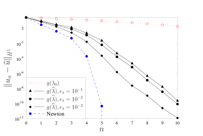
(b)

Figure 1: (a) (Shifted) energy $e(u_{n})-e({\widehat{u}})$ and (b) the $H^{1}$ approximation error $\|u_{n}-{\widehat{u}}\|_{H^{1}}$ as functions of the iteration count $n$ where the optimal gradients $g({\widehat{\lambda}})$ are obtained using Algorithm 3 with $N=50$ and different tolerances $\epsilon_{\lambda}=10^{-1},10^{-2},10^{-3}$. For comparison, the results obtained using standard Sobolev gradients $g(\lambda_{0})$ with a constant weight $\lambda_{0}=10$ and with Newton’s method, cf. Algorithm 2, are also presented.

5.2 Analysis of the effect of the dimension $N$ of the approximation space $\Lambda$

The results concerning the effect of $N$ on the performance of approach (b) are compared with the data for approaches (a) and (c) in Figures 3a and 3b for the (shifted) energy $e(u_{n})-e(\widehat{u})$ and the $H^{1}$ approximation error $\|u_{n}-{\widehat{u}}\|_{H^{1}}$, respectively. We observe that, when optimal gradients $g({\widehat{\lambda}})$ are used, both $e(u_{n})-e({\widehat{u}})$ and $\|u_{n}-{\widehat{u}}\|_{H^{1}}$ initially reveal a quadratic convergence, similar to the behavior of these quantities in Newton’s method, followed at later iterations by a linear convergence, typical of the standard gradient method. In the light of Theorem 3.4, cf. estimate (32), this observation can be explained by the fact that at early iterations dominant components of the error $(u_{n}-{\widehat{u}})$ are contained in the subspaces $T_{u_{n}}$ where the optimal gradients $g({\widehat{\lambda}})$ are consistent with Newton’s steps $h$, cf. Remark 2.2. Then, once these error components are eliminated, at later iterations the error $(u_{n}-{\widehat{u}})$ is dominated by components in directions orthogonal to $T_{u_{n}}$ where the optimal gradients $g({\widehat{\lambda}})$ do not well reproduce the Newton steps $h$. In Figures 3a and 3b we also see that the convergence improves as the dimension $N$ is increased until it saturates for $N$ large enough (here $N\gtrapprox 25)$. This could be explained by the conjecture that increasing $N$ above a certain limit (approximately $25$ in this case) does not increase the “effective” dimension of $T_{u_{n}}$ in $H$ anymore (such a possibility is allowed by the error analysis presented in Section 3.1).

In this context it is also interesting to investigate the evolution of the spatial structure of the optimal weights ${\widehat{\lambda}}(x)$ and these results are shown for different values of $N$ at an early ($n=2$) and a later ($n=8$) iteration in Figures 3a and 3b, respectively. In the first case ($n=2$ corresponding to the quadratic convergence) we see that the optimal weights ${\widehat{\lambda}}(x)$ converge to a well-defined profile as $N$ increases, which features a number of distinct “spikes”. On the other hand, at later iterations ($n=8$ corresponding to the linear regime) the convergence of the optimal weights ${\widehat{\lambda}}(x)$ with $N$ is less evident and the resulting profiles tend to be more uniform.

   

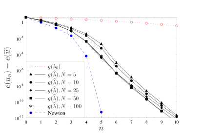
(a)

(b)

Figure 2: (a) (Shifted) energy $e(u_{n})-e({\widehat{u}})$ and (b) the $H^{1}$ approximation error $\|u_{n}-{\widehat{u}}\|_{H^{1}}$ as functions of the iteration count $n$ for different dimensions $N$ where the optimal gradients $g({\widehat{\lambda}})$ are obtained with Algorithm 3. For comparison, the results obtained using standard Sobolev gradients $g(\lambda_{0})$ with a constant weight $\lambda_{0}=10$ and with Newton’s method, cf. Algorithm 2, are also presented.

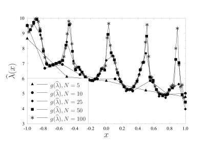
(a)

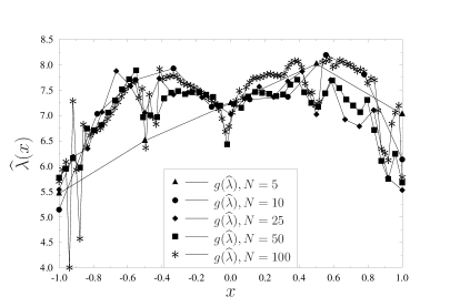
(b)

Figure 3: Optimal weights ${\widehat{\lambda}}(x)$ as functions of $x$ obtained for different $N$: (a) an early ($n=2$) iteration and (b) a late ($n=8$) iteration of Algorithm 3, cf. Figure 3.

We want to highlight the case when $N=1$ and space $H$ is endowed with the inner product redefined as in (25). As shown in Remark 2.5, in such circumstances the optimal $\lambda$ can be found analytically, cf. relation (26), at essentially no cost and the iterations produced by Algorithm 1 do not depend on the step size $\kappa$. The results obtained with this approach and using the optimal gradients $g({\widehat{\lambda}})$ defined in terms of the inner product (9) are compared in Figures 4a and 4b for the (shifted) energy $e(u_{n})-e(\widehat{u})$ and the $H^{1}$ approximation error $\|u_{n}-{\widehat{u}}\|_{H^{1}}$, respectively. As is evident from these figures, the performance of the approaches corresponding to the two definitions of the inner product, (9) and (25), is comparable and in both cases much better than when a fixed weight $\lambda_{0}$ is used. We stress that in the case corresponding to the inner product (25) determination of the optimal $\lambda$ does not require an iterative solution.

 

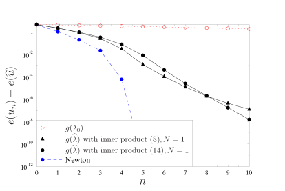
(a)

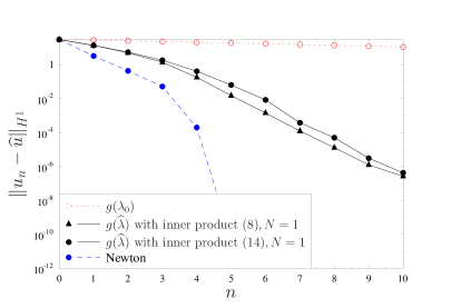
(b)

Figure 4: (a) (Shifted) energy $e(u_{n})-e({\widehat{u}})$ and (b) the $H^{1}$ approximation error $\|u_{n}-{\widehat{u}}\|_{H^{1}}$ as functions of the iteration count $n$ for the case when $N=1$ and the optimal gradients $g({\widehat{\lambda}})$ are obtained using the inner product definitions (9) combined with Algorithm 3 and (25) combined with the explicit relation (26). For comparison, the results obtained using standard Sobolev gradients $g(\lambda_{0})$ with a constant weight $\lambda_{0}=10$ and with Newton’s method, cf. Algorithm 2, are also presented. The step size used in these calculations is $\kappa=25$.

5.3 Analysis of the robustness of approach (b) with respect to variations of the basis functions defining $\eta$

This analysis is performed by constructing basis functions $\{\ell^{i}\}_{i=1}^{N}$ based on grid points distributed randomly with an uniform probability distribution over the interval $(-1,1)$, except for the leftmost and the rightmost grid points which are always at $x=\pm 1$. The results obtained in several realizations with $N=5$ are compared to the reference case of basis functions constructed based on equispaced grid points as well as with the results obtained with approaches (a) and (c) in Figures 5a and 5b for the (shifted) energy $e(u_{n})-e(\widehat{u})$ and the $H^{1}$ approximation error $\|u_{n}-{\widehat{u}}\|_{H^{1}}$, respectively. One can see in these figures that, expect for one realization corresponding to a very special distribution of the grid points, the convergence is little affected by the choice of the basis $\{\ell^{i}\}_{i=1}^{N}$.

 

(a)

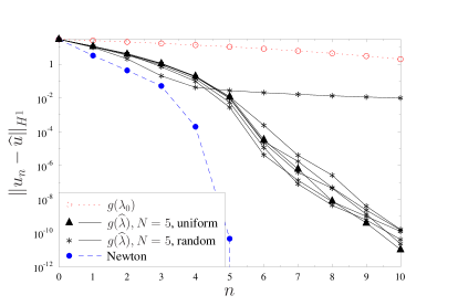
(b)

Figure 5: (a) (Shifted) energy $e(u_{n})-e({\widehat{u}})$ and (b) the $H^{1}$ approximation error $\|u_{n}-{\widehat{u}}\|_{H^{1}}$ as functions of the iteration count $n$ for the case when $N=5$ and the optimal gradients $g({\widehat{\lambda}})$ are obtained with Algorithm 3 using uniform and random distributions of grid points defining the basis functions $\{\ell^{i}\}_{i=1}^{N}$. For comparison, the results obtained using standard Sobolev gradients $g(\lambda_{0})$ with a constant weight $\lambda_{0}=10$ and with Newton’s method, cf. Algorithm 2, are also presented.

5.4 Analysis of the performance of a simplified version of Algorithm 4

Finally, we consider approach (d) where the optimal weights ${\widehat{\lambda}}(x)$ and the corresponding optimal gradients $g({\widehat{\lambda}})$ are determined with Algorithm 4 simplified as follows. The complexity analysis presented in Section 4.3 shows that Algorithm 4 may be quite costly from the computational point of view when $N\gg 1$. To alleviate this difficulty, we consider its simplified version where only one iteration ($N_{n}=1$) is performed on system (53) in which the “test” functions $g^{\prime}_{i}$, $i=1,\dots,N$, are assumed not to depend on $\lambda$ (or $\eta$). In other words, since instead of $g^{\prime}_{i}(\eta)$, $i=1,\dots,N$, the functions $g^{\prime}_{i}(\eta_{0})$ are used to obtain expressions for $[F(\eta)]_{i}$, $i=1,\dots,N$, in (53), the second derivatives $g^{\prime\prime}_{ij}$ are eliminated from the Hessian $[DF(\eta)]_{ij}$, $i,j=1,\dots,N$ in (55), which very significantly reduces the computational cost. The results obtained with this simplified approach are shown in Figures 6a and 6b, respectively, for the decrease of the (shifted) energy $e(u_{n})-e({\widehat{u}})$ and for the decrease of the $H^{1}$ approximation error $\|u_{n}-{\widehat{u}}\|_{H^{1}}$. In these figures we observe general trends qualitatively similar to those evident in Figures 3a and 3b, except that the convergence is slower and the transition from the quadratic to linear convergence tends to occur at earlier iterations.

 

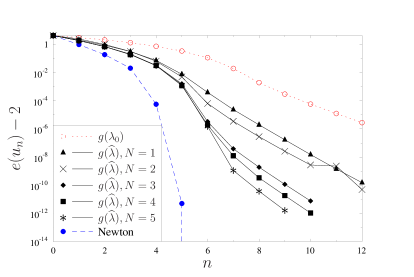
(a)

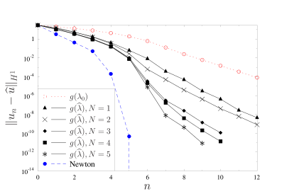
(b)

Figure 6: (a) (Shifted) energy $e(u_{n})-e({\widehat{u}})$ and (b) the $H^{1}$ approximation error $\|u_{n}-{\widehat{u}}\|_{H^{1}}$ as functions of the iteration count $n$ for different dimensions $N$ where the optimal gradients $g({\widehat{\lambda}})$ are obtained with the simplified version of Algorithm 4 described above. For comparison, the results obtained using standard Sobolev gradients $g(\lambda_{0})$ with a constant weight $\lambda_{0}=10$ and with Newton’s method, cf. Algorithm 2, are also presented.

6 Conclusions

We have developed a gradient-type numerical approach for unconstrained optimization problems in infinite-dimensional Hilbert spaces. Our method consists in finding an optimal inner product among a family of equivalent inner products parameterized by a space-dependent weight $\lambda$ function. The optimal weight ${\widehat{\lambda}}$ solves a nonlinear optimization problem in a finite dimensional subspace. Rigorous analysis demonstrates that, in addition to the linear convergence characterizing the standard gradient method, the proposed approach also attains quadratic convergence in the sense that the projection error in a finite-dimensional subspace generated in the process decreases quadratically. Or, equivalently, in this finite dimensional subspace, the optimal gradients and Newton’s steps are equivalent. The dimension of these subspaces is determined by the number $N$ of discrete degrees of freedom parameterizing the inner products through the weight $\lambda$.

This analysis is confirmed by numerical experiments, performed based on a simple optimization problem in a setting mimicking high spatial resolution. More specifically, at early iterations both the minimized energy and the error with respect to the exact solution exhibit quadratic convergence followed by the linear convergence at later iterations. The behavior of the proposed method also reveals expected trends with variations of the numerical parameters, namely, the dimension of the space in which the optimal weights ${\widehat{\lambda}}$ are constructed, properties of the basis in this space and the accuracy with which the inner optimization problems are solved. In all cases the convergence of the proposed approach is much faster than obtained using Sobolev gradients with fixed weights. For the ease of analysis and comparisons we focused on a gradient-descent method with a fixed step size $\kappa$, but it can be expected that a similar behavior will also occur when the step size is determined adaptively through suitable line minimization.

The complexity analysis performed in Section 4.3 indicates that the per-iteration cost of the proposed approach and of the standard Sobolev gradient method have the same order if, for example, the energy depends on a elliptic PDE. When the dimension of weight space is $N=1$ and the inner product does not have the $L^{2}$ term, cf. (25), then the optimal weight is given explicitly, eliminating the need for its numerical determination. In this particular case the proposed approach has some similarity to the Barzilai-Borwein algorithm [3] and produces iterates which do not depend on the step size in the gradient method. The computational cost of the proposed approach is also significantly reduced when Algorithm 4 is used in a simplified form, as described in Section 5. We thus conclude that the gradient-descent method from Algorithm 1 combined with Algorithms 3 and 4 used to find optimal gradients are promising approaches suitable for large-scale optimization problems and applications to some such problems will be investigated in the near future.

Our approach based on optimal gradients differs from the family of quasi-Newton methods in that instead of approximating the full Hessian using gradients from earlier iterations, see for example [11], it relies on computing the action of the exact Hessian and gradients, but only on a few judiciously selected directions, and then matching them by appropriately choosing the inner product. Consequently, the resulting algebraic problem is of a much smaller dimension thereby avoiding complications related to poor conditioning and computational cost.

Finally, we believe that the analysis and results presented here explain the acceleration of gradient minimization reported for a range of different problems in [13, 14, 16, 15, 12, 7] when Sobolev gradients with suitable (constant) weights were used. Moreover, our work also provides a rational and constructive answer to the open problem of finding an optimal form of the inner product defining the Sobolev gradients.

References

- [1] R. A. Adams and J. F. Fournier, “Sobolev Spaces”, Elsevier, (2005).
- [2] D. Ayala and B. Protas, “Extreme vortex states and the growth of enstrophy in three-dimensional incompressible flows”, Journal of Fluid Mechanics 818, 772–806, 2017.
- [3] J. Barzilai, J. M. Borwein, Two-Point Step Size Gradient Methods, IMA Journal of Numerical Analysis, Volume 8, Issue 1, 1 January 1988, Pages 141-148,
- [4] H. Brezis, Functional Analysis, Sobolev Spaces and Partial Differential Equations, Springer
- [5] Ph. G. Ciarlet, Introduction à l’analyse matricielle et à l’optimisation, Dunod, Paris, 1998
- [6] Driscoll, T. A., Hale, N. & Trefethen, L. N. 2014 Chebfun Guide, Pafnuty Publications edn. Oxford.
- [7] I. Danaila and P. Kazemi “A new Sobolev gradient method for direct minimization of the Gross-Pitaevskii energy with rotation”, SIAM Journal on Scientific Computing 32, 2447–2467 (2010).
- [8] P. Kazemi and I. Danaila, “Sobolev gradients and image interpolation”, SIAM Journal on Imaging Sciences 5, 601–624 (2012).
- [9] C. T. Kelley, “Solving nonlinear equations with Newton’s method: Fundamentals of algorithms”, SIAM, Philadelphia. (2003).
- [10] J. W. Neuberger, Sobolev Gradients and Differential Equations, Springer, (2010).
- [11] J. Nocedal and S. Wright, “Numerical Optimization”, Springer, (2002).
- [12] A. Majid and S. Sial, “Application of Sobolev gradient method to Poisson-Boltzmann system ”, Journal of Computational Physics 229, 5742-5754, 2010.
- [13] B. Protas, T. R. Bewley and G. Hagen, “A comprehensive framework for the regularization of adjoint analysis in multiscale PDE systems”, Journal of Computational Physics 195(1), 49-89, 2004.
- [14] B. Protas “Adjoint–Based Optimization of PDE Systems with Alternative Gradients” Journal of Computational Physics 227, 6490–6510, 2008.
- [15] R. J. Renka, “Geometric curve modeling with Sobolev gradients”, in J. W. Neuberger (Ed.), Sobolev Gradients and Differential Equations, Springer Lecture Notes in Mathematics 1670, 199–208, 2010.
- [16] N. Raza, S. Sial, S. S. Siddiqi and T. Lookman, “Energy minimization related to the nonlinear Schrödinger equation”, Journal of Computational Physics 228, 2572-2577, 2009.
- [17] I. Farago and J. Karátson, “Numerical Solution of Nonlinear Elliptic Problems Via Preconditioning Operators: Theory and Applications”, Nova Science, (2002).
- [18] J. Karátson and J. W. Neuberger, “Newton’s method in the context of gradients”, Electronic Journal of Differential Equations 124, 1–13, (2007).
- [19] R. Temam, Navier-Stokes Equations, AMS Chelsea Publishing, AMS, 2000