Abstract:

High temperature gases, for instance in hypersonic reentry flows, show complex phenomena like excitation of rotational and vibrational energy modes, and even chemical reactions. For flows in the continuous regime, simulation codes use analytic or tabulated constitutive laws for pressure and temperature. In this paper, we propose a BGK model which is consistent with any arbitrary constitutive laws, and which is designed to make high temperature gas flow simulations in the rarefied regime. A Chapman-Enskog analysis gives the corresponding transport coefficients. Our approach is illustrated by a numerical comparison with a compressible Navier-Stokes solver with rotational and vibrational non equilibrium. The BGK approach gives a deterministic solver with a computational cost which is close to that of a simple monoatomic gas.

Keywords:

rarefied gas dynamics, polyatomic gas, BGK model, real gas effect, second principle

Contents

1. 1 Introduction
2. 2 Polyatomic BGK model
3. 3 High temperature gases
   1. 3.1 Vibrations
      1. 3.1.1 Example 1: dioxygen
      2. 3.1.2 Example 2: air
   2. 3.2 Chemical reactions
4. 4 BGK models for high temperature gases
   1. 4.1 A polyatomic BGK model for a variable number of degrees of freedom
   2. 4.2 A more general BGK model for arbitrary constitutive laws
   3. 4.3 Compressible Navier-Stokes asymptotics
      1. 4.3.1 Comments on this model
      2. 4.3.2 Non-dimensional form
      3. 4.3.3 Conservation laws
      4. 4.3.4 Euler equations
      5. 4.3.5 Navier-Stokes equation
   4. 4.4 Entropy
   5. 4.5 Reduced model
5. 5 Numerical results
   1. 5.1 Moderate temperature flow: vibrating molecules
   2. 5.2 High temperature flow: reacting gas
6. 6 Conclusion
7. A Gaussian integrals

1 Introduction

For atmospheric reentry of space vehicles, it is important to estimate the heat flux at the solid wall of the vehicle. In such hypersonic flows, the temperature is very large, and the air flow, which is a mixture of monoatomic and polyatomic gases, is modified by chemical reactions. The characteristics of the mixture (viscosity and specific heats) then depend on its temperature (see [25]).

One way to take into account this variability is to use appropriate constitutive laws for the air. For instance, quantum mechanics allows to derive a relation between internal energy and temperature that accounts for activation of vibrational modes of the molecules (see [1]). When the temperature is larger, chemical reactions occur, and if the flow is in chemical equilibrium, empirically tabulated laws can be used to compute all the thermodynamical quantities (pressure, entropy, temperature, specific heats) in terms of density and internal energy, like the one given in [1, 16]. These laws give a closure of the compressible Navier-Stokes equations, that are used for simulations in the continuous regime, at moderate to low altitudes (see, for example, [24]).

In high altitude, the flow is in the rarefied or transitional regime, and it is described by the Boltzmann equation of Rarefied Gas Dynamics, also called the Wang-Chang-Uhlenbeck equation in case of a reacting mixture. This equation is much too complex to be solved by deterministic methods, and such flows are generally simulated by the DSMC method [12]. However, it is attractive to derive simplified kinetic models that account for high temperature effects, in order to obtain alternative and deterministic solvers: for such computations, it is necessary to capture dense zones with high temperatures and very rarefied zones with low temperatures. Up to our knowledge, the first attempt to introduce non ideal constitutive laws into a kinetic model has recently been published in [26]. In this article, the authors define the constant volume specific heat $c_{v}$ as a third-order polynomial function of the temperature of the gas, and derive a mesoscopic model based on the moment approach. A similar approach is proposed in [18] that gives a correct Prandtl number. Simplified Boltzmann models for mixtures of polyatomic gases have also been proposed in [2, 8, 14], however, high temperature effects are not addressed in these references.

In this paper, our goal is to construct models that are able to capture macroscopic effects as well as kinetic effects at a reasonable numerical cost, for an application to reentry flows. We propose two ways to include high temperature effects (vibrational modes, chemical reactions) in a generalized BGK model.

First, we show that vibrational modes can be taken into account by using a temperature dependent number of degrees of freedom. This can be used in a BGK model for polyatomic gases, but we show that the choice of the variable used to describe the internal energy of the molecules is fundamental here. This model allows us to simulate a mixture of rarefied polyatomic gases (like the air) with rotational and vibrational non equilibrium, with a single distribution function for the mixture. As a consequence, we are able to simulate a polyatomic gas flow with a non-constant specific heat.

Then we propose a more general BGK model that can be used to describe a rarefied flow with both vibrational excitation and chemical reactions, at chemical equilibrium, based on arbitrary constitutive laws for pressure and temperature. Our BGK model is shown to be consistent with the corresponding Navier-Stokes model in the small Knudsen number limit. Finally, the internal energy variable of our BGK model can be eliminated by the standard reduced distribution technique [17]: this gives a kinetic model for high temperature polyatomic gases with a computational complexity which is close to that of a simple monoatomic model.

Up to our knowledge, the model proposed in this work is the first Boltzmann model equation that allows for realistic equations of state and includes concentration effects in the thermal flux. We point out that this article is a first step towards a correct computation of the parietal heat flux: since we use a BGK model, it is clear that our model does not have a correct Prandtl number, as usual. This might be solved by using the ES-BGK approach [3, 22, 23] to capture the correct relaxation times for energy and fluxes [19].

The outline of our paper is the following. First we remind a standard BGK model for polyatomic gases in section 2. Then, in section 3, we explain how high temperature effects are taken into account to define the internal number of degrees of freedom of molecules and generalized constitutive laws. A first BGK model is proposed to allow for vibrational mode excitation with a temperature dependent number of degrees of freedom in section 4.1. This model is extended to allow for arbitrary constitutive laws for pressure and temperature in section 4.2, and this model is also analyzed by the Chapman-Enskog expansion. Some features of our new model are illustrated by a few numerical simulations in section 5.

2 Polyatomic BGK model

For standard temperatures, a polyatomic perfect gas can be described by the mass distribution function $F(t,x,v,\varepsilon)$ that depends on time $t$, position $x$, velocity $v$, and internal energy $\varepsilon$. The internal energy is described with a continuous variable, and takes into account rotational modes. The corresponding number of degrees of freedom for rotational modes is $\delta$ (see [10]).

Corresponding macroscopic quantities mass density $\rho$, velocity $u$, and specific internal energy $e$, are defined through the first 5 moments of $F$ with respect to $v$ and $\varepsilon$:

$$\rho(t,x) =\langle\langle F\rangle\rangle,$$ (1)

$$\rho u(t,x) =\langle\langle vF\rangle\rangle,$$ (2)

$$\rho e(t,x) =\langle\langle(\frac{1}{2}|v-u|^{2}+\varepsilon)F\rangle\rangle,$$ (3)

where $\langle\langle\phi\rangle\rangle=\int_{{\mathbb{R}}^{3}}\int_{0}^{+\infty}\phi(v,\varepsilon)\,dvd\varepsilon$ denotes the integral of any scalar or vector-valued function $\phi$ with respect to $v$ and $\varepsilon$. The specific internal energy take into account translational and rotational modes. Other macroscopic quantities can be derived from these definitions. The temperature is $T$ is such that $e=\frac{3+\delta}{2}RT$, where $R$ is the gas constant. The pressure is given by the perfect gas equation of state (EOS) $p=\rho RT$.

For a gas in thermodynamic equilibrium, the distribution function reaches a Maxwellian state, defined by

$$M[F]=\frac{\rho}{(2\pi RT)^{\frac{3}{2}}}\exp\left(-\frac{|v-u|^{2}}{2RT}\right)\Lambda(\delta)\left(\frac{\varepsilon}{RT}\right)^{\frac{\delta}{2}-1}\frac{1}{RT}\exp\left(-\frac{\varepsilon}{RT}\right),$$ (4)

where $\rho$, $u$, and $T$ are defined above. The constant $\Lambda(\delta)$ is a normalization factor defined by $\Lambda(\delta)=1/\Gamma(\frac{\delta}{2})$, so that $M[F]$ has the same 5 moments as $F$ (see above).

The simplest BGK model that can be derived from this description is the following

$$\partial_{t}F+v\cdot\nabla_{x}F=\frac{1}{\tau}(M[F]-F),$$ (5)

where $\tau$ is a relaxation time (see below).

The standard Chapman-Enskog expansion shows that this model is consistent, with an error which is of second order with respect to the Knudsen number, to the following compressible Navier-Stokes equations

$$\partial_{t}\rho+\nabla\cdot\rho u=0$$

$$\partial_{t}\rho u+\nabla\cdot(\rho u\otimes u)+\nabla p=-\nabla\cdot\sigma$$

$$\partial_{t}E+\nabla\cdot((E+p)u)=-\nabla\cdot q-\nabla\cdot(\sigma u),$$

where $\sigma=-\mu(\nabla u+(\nabla u)^{T}-\frac{2}{3+\delta}\nabla\cdot u\,Id)$ is the shear stress tensor and $q=-\kappa\nabla T$ is the heat flux. The transport coefficients $\mu$ and $\kappa$ are linked to the relaxation time by the relations $\mu=\tau p$ and $\kappa=\mu c_{p}$, where the specific heat at constant pressure is $c_{p}=\frac{5+\delta}{2}R$. Actually, these relations define the correct value that has to be given to the relaxation time $\tau$ of (5), which is

$$\tau=\frac{\mu}{p},$$ (6)

where the viscosity is given by a standard temperature dependent law like $\mu(T)=\mu_{ref}(\frac{T}{T_{ref}})^{\omega}$ (see [7]). This implies that the Prandtl number ${\rm Pr}=\frac{\mu c_{p}}{\kappa}$ is equal to $1$. This incorrect result (it should be close to $\frac{5}{7}$ for a diatomic gas, for instance) is due to the fact that the BGK model contains only one relaxation time. Instead it would be more relevant to include at least three relaxation times in the model to allow for various different time scales (viscous versus thermal diffusion time scale, translational versus rotational energy relaxation rates). It is possible to take these different time scales into account by using the ESBGK polyatomic model (see [3]), or the Rykov model (see [20] and the references therein). See also multiple relaxation time BGK models developed for polyatomic gases in [4, 5]. However, in this work, the derivation of a model for high temperature gases is based on this simple polyatomic BGK model (with a single relaxation time).

Note that this model is generally simplified by using the variable $I$ such that the internal energy of a molecule is $\varepsilon=I^{\frac{2}{\delta}}$ (see [3]). Then the corresponding distribution ${\cal F}(t,x,v,I)$ is defined such that ${\cal F}dxdvdI=Fdxdvd\varepsilon$, which gives ${\cal F}=I^{\frac{2}{\delta}-1}F$. The macroscopic quantities are defined by

$$\rho(t,x)=\langle\langle{\cal F}\rangle\rangle,\qquad\rho u(t,x)=\langle\langle v{\cal F}\rangle\rangle,\qquad\rho e(t,x)=\langle\langle(\frac{1}{2}|v-u|^{2}+I^{\frac{2}{\delta}}){\cal F}\rangle\rangle,$$

where now $\langle\langle\phi\rangle\rangle=\int_{{\mathbb{R}}^{3}}\int_{0}^{+\infty}\phi(v,I)\,dxdI$. The corresponding Maxwellian, which is simpler, is

$${\cal M}[{\cal F}]=\frac{\rho}{(2\pi RT)^{\frac{3}{2}}}\exp\left(-\frac{|v-u|^{2}}{2RT}\right)\frac{2}{\delta}\Lambda(\delta)\frac{1}{(RT)^{\frac{\delta}{2}}}\exp\left(-\frac{I^{\frac{2}{\delta}}}{RT}\right).$$ (7)

The corresponding BGK equation is

$$\partial_{t}{\cal F}+v\cdot\nabla_{x}{\cal F}=\frac{1}{\tau}({\cal M}[{\cal F}]-{\cal F}),$$ (8)

which is equivalent to (5).

Moreover, note that these models can be derived from [11]: in that paper, the authors first give a Boltzmann collision operator for polyatomic gases deduced from the Borgnakke-Larsen model. In this model, the internal energy variable $\varepsilon$ is described by a variable $I$ such that $I=\sqrt{\varepsilon}$. By using the corresponding Maxwellian, it is easy to derive a single relaxation time BGK model. When this model is written with $\varepsilon$, we exactly get model (5).

In the same paper [11], the authors propose a second Boltzmann collision operator based on a model for a monoatomic gas in higher dimension, with an internal variable $w$ that lives in a $\delta$-dimension space, where $\delta$ is the number of internal degrees of freedom. The internal energy of the model is $\varepsilon=|w|^{2}$. This model is written in polar coordinates $w=I\theta$, where $I$ is the norm of $w$ (and hence again the square root of $\varepsilon$), and $\theta$ is the polar angle, and then it is reduced by integration with respect to $\theta$. The authors get a Boltzmann collision operator in which the distribution function is multiplied by a weight function $\phi(I)=I^{\delta-1}$. Again, a BGK model can be derived from this formulation, but it is different from models (5) and (7). The resulting model has been extended by several authors to get BGK models for non polytropic gases (see section 3). However, in the case of polytropic gases (i.e. constant $\delta$), this model can easily be shown to be equivalent to our model (5).

3 High temperature gases

When the temperature of the gas is larger, new phenomena appear (vibration, chemical reactions, ionization). For instance, for dioxygen, at $800$K, the molecules begin to vibrate, and chemical reactions occur for much larger temperatures (for instance, dissociation of $O_{2}$ into $O$ starts at $2500$K).

The next sections explain how some of these effects (vibrations and chemical reactions) can be taken into accounts in terms of EOS and number of internal degrees of freedom.

3.1 Vibrations

Of course, the definition of the specific internal energy must account for vibrational energy. A possible way to do so is to increase the number of internal degrees of freedom $\delta$, that now accounts for rotational and vibrational modes. However, a result of quantum mechanics implies that this number of degrees of freedom is not an integer anymore, and that it is even not a constant (it is temperature dependent), see the examples below. Vibrating gases have other properties that make them quite different to what is described by the standard kinetic theory of monoatomic gases. For instance, the specific heat at constant pressure $c_{p}$ becomes temperature dependent. However, vibrating gases can still be considered as perfect gases, so that the perfect EOS $p=\rho RT$ still holds (in fact, such gases are called thermally perfect gases, see [1]).

Now we give two examples of gases with vibrational excitation, and we explain how their number of internal degrees of freedom is defined.

3.1.1 Example 1: dioxygen

At equilibrium, translational $e_{tr}$ and rotational $e_{rot}$ specific energies can be defined by

$$e_{tr}=\frac{3}{2}RT\quad\text{ and }\quad e_{rot}=RT.$$

This shows that a molecule of dioxygen has $3$ degrees of freedom for translation, and $2$ for rotation. By using quantum mechanics [1], vibrational specific energy $e_{vib}$ is found to be

$$e_{vib}=\frac{T^{vib}_{O_{2}}/T}{\exp(T^{vib}_{O_{2}}/T)-1}RT,$$

where $T^{vib}_{O_{2}}=2256$K is a reference temperature.

The number of “internal” degrees of freedom $\delta$, related to rotation and vibration modes only, is defined such that the total specific internal energy $e$ is

$$e=e_{tr}+e_{rot}+e_{vib}=\frac{3+\delta}{2}RT.$$

By combining this relation with the relations above, we find that $\delta$ is actually temperature dependent, and defined by

$$\delta(T)=2+2\frac{T^{vib}_{O_{2}}/T}{\exp(T^{vib}_{O_{2}}/T)-1}.$$

Accordingly, the specific heat at constant pressure $c_{p}$, which is defined by $dh=c_{p}dT$, where the enthalpy is $h=e+\frac{p}{\rho}$, can be computed as follows. Since $p=\rho RT$, we find $h=\frac{5+\delta(T)}{2}RT$, and hence the enthalpy depends on $T$ only, through a nonlinear relation. This means that $c_{p}=h^{\prime}(T)$ is not a constant anymore, while we have $c_{p}=\frac{5+\delta}{2}R$ without vibrations. Finally, note that the relation that defines the temperature $T$ through the internal specific energy $e=\frac{3+\delta(T)}{2}RT$ now is nonlinear (it has to be inverted numerically to find $T$).

3.1.2 Example 2: air

The air at moderately high temperatures ($T<2500$K) is a non-reacting mixture of nitrogen $N_{2}$ and dioxygen $O_{2}$. To simplify, assume that their mass concentrations are $c_{N_{2}}=75\%$ and $c_{O_{2}}=25\%$. These two species are perfect gases with their own gas constants $R_{N_{2}}$ and $R_{O_{2}}$. The gas constant $R$ of the mixture can be defined by $R=c_{N_{2}}R_{N_{2}}+c_{O_{2}}R_{O_{2}}$ (see [1]).

The specific internal energy is defined by $e=c_{O_{2}}e_{O_{2}}+c_{N_{2}}e_{N_{2}}$. The energy of each species can be computed like in our first example (see section 3.1.1), and we find:

$$e_{N_{2}}=\frac{3+\delta_{N_{2}}(T)}{2}R_{N_{2}}T\qquad\text{and}\qquad e_{O_{2}}=\frac{3+\delta_{O_{2}}(T)}{2}R_{O_{2}}T,$$

where the number of internal degrees of freedom of each species are

$$\delta_{N_{2}}(T)=2+2\frac{T^{vib}_{N_{2}}/T}{\exp(T^{vib}_{N_{2}}/T)-1}\qquad\text{and}\qquad\delta_{O_{2}}(T)=2+2\frac{T^{vib}_{O_{2}}/T}{\exp(T^{vib}_{O_{2}}/T)-1},$$ (9)

with $T^{vib}_{N_{2}}=3373$K and $T^{vib}_{O_{2}}=2256$K. Then the specific internal energy of the mixture is

$$\begin{split}e&=c_{O_{2}}\frac{3+\delta_{O_{2}}(T)}{2}R_{O_{2}}T+c_{N_{2}}\frac{3+\delta_{N_{2}}(T)}{2}R_{N_{2}}T\\ &=\frac{3}{2}RT+\frac{1}{2}(c_{O_{2}}\delta_{O_{2}}(T)R_{O_{2}}+c_{N_{2}}\delta_{N_{2}}(T)R_{N_{2}})T\\ &=\frac{3+\delta(T)}{2}RT\end{split}$$

with the number of internal degrees of freedom given by

$$\begin{split}\delta(T)&=\frac{c_{O_{2}}\delta_{O_{2}}(T)R_{O_{2}}+c_{N_{2}}\delta_{N_{2}}(T)R_{N_{2}}}{R}\\ &=2+\frac{2}{R}\left(c_{O_{2}}R_{O_{2}}\frac{T^{vib}_{O_{2}}/T}{\exp(T^{vib}_{O_{2}}/T)-1}+c_{N_{2}}R_{N_{2}}\frac{T^{vib}_{N_{2}}/T}{\exp(T^{vib}_{N_{2}}/T)-1}\right).\end{split}$$ (10)

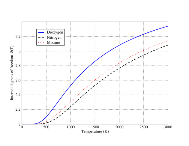
Figure 1: Internal degrees of freedom as a function of the temperature

We show in figure 1 the number of internal degrees of freedom for each species and for the whole mixture. For all gases, $\delta$ is equal to $2$ below $500$K, which means that only the rotational modes are excited: each species is a diatomic gas with 2 degrees of freedom of rotation, and the mixture behaves like a diatomic gas too. Then the number of degrees of freedom increases with the temperature, and is greater than $3$ for $T=3000$K. At this temperature, the number of degrees of freedom for vibrations is around $1$. Note that in addition to this graphical analysis, it can be analytically proved that all the $\delta$ computed here are increasing functions of $T$.

3.2 Chemical reactions

When chemical reactions have to be taken into account (for the air, this starts at $2500$K), the perfect gas EOS still holds for each species, but the EOS for the reacting mixture is less simple. To avoid the numerical solving of the Navier-Stokes equations for all the species, in the case of an equilibrium chemically reacting gas, it is convenient to use instead a Navier-Stokes model for the mixture (considered as a single species), for which tabulated EOS $p=p(\rho,e)$ and even a tabulated temperature law $T=T(\rho,e)$ are used (see [1], chapter 11).

More precisely, it can be proved that for a mixture of thermally perfect gases in chemical equilibrium, with a constant atomic nuclei composition, two state variables, like $\rho$ and $e$, are sufficient to uniquely define the chemical composition of the mixture. Let us precise what this means, with notations that will be useful in the paper. For each species of the mixture, numbered with index $i$:

• its concentration $c_{i}$ depends on $\rho$ and $e$ only: $c_{i}=c_{i}(\rho,e)$ ;

• its pressure $p_{i}$ satisfies the usual perfect gas law: $p_{i}=\rho_{i}R_{i}T$, where $R_{i}$ is the gas constant of the species and $\rho_{i}=c_{i}(\rho,e)\rho$, so that $p_{i}=p_{i}(\rho,e)$ ;

• its specific energy $e_{i}$ and enthalpy $h_{i}$ depend on $T$ only: $e_{i}=e_{i}(T)$ and $h_{i}=h_{i}(T)$, where $e_{i}(T)=\frac{3+\delta_{i}(T)}{2}R_{i}T+e_{i}^{f,0}$, with $e_{i}^{f,0}$ is the energy of formation of the $i$th molecule and $\delta_{i}(T)$ is the number of activated internal degrees of freedom of the molecule that might depend on the temperature, see the previous sections ($\delta_{i}=0$ for monoatomic molecules).

For compressible Navier-Stokes equations for an equilibrium chemically reacting mixture, these quantities are not necessary. Instead, it is sufficient to define (with analytic formulas or tables):

• the total pressure $p=\sum_{i}p_{i}(\rho,e)$ so that $p=p(\rho,e)=\rho R(\rho,e)T$, with $R(\rho,e)=\sum_{i}c_{i}(\rho,e)R_{i}$ ;

• the temperature $T$, through the relation $e=\sum_{i}c_{i}(\rho,e)e_{i}(T)$, so that $T=T(\rho,e)$ ;

• the total specific enthalpy $h=\sum_{i}c_{i}h_{i}$, so that $h=h(\rho,e)=e+\frac{p(\rho,e)}{\rho}$.

We refer to [1] for details on this subject.

4 BGK models for high temperature gases

4.1 A polyatomic BGK model for a variable number of degrees of freedom

In this section, we propose an extension of the polyatomic BGK model (5) to take into account temperature dependent number of internal degrees of freedom, like in examples of sections 3.1.1 and 3.1.2.

This extension (already obtained in [21]) is quite obvious, since we just replace the constant $\delta$ in (4) by the temperature dependent $\delta(T)$. For completeness, this model is given below:

$$\partial_{t}F+v\cdot\nabla_{x}F=\frac{1}{\tau}(M[F]-F),$$ (11)

with

$$M[F]=\frac{\rho}{(2\pi RT)^{\frac{3}{2}}}\exp\left(-\frac{|v-u|^{2}}{2RT}\right)\Lambda(\delta(T))\left(\frac{\varepsilon}{RT}\right)^{\frac{\delta(T)}{2}-1}\frac{1}{RT}\exp\left(-\frac{\varepsilon}{RT}\right).$$ (12)

The macroscopic quantities are defined by (1)–(3), while the temperature $T$ is defined by

$$e=\frac{3+\delta(T)}{2}RT.$$ (13)

Indeed, this implicit relation is invertible if, for instance, $\delta(T)$ is an increasing function of $T$. This is true, at least for the examples shown in section 3.1.2: it can easily be shown that equations (9) and (10) define increasing functions of $T$. Finally, the relaxation time $\tau$ is given by (6) with $p=\rho RT$.

The same model has been proposed independently in [18], and extended to an ES-BGK version to have correct transport coefficients. Note that in [18], the temperature dependent number of degrees of freedom $\delta(T)$ is constructed through a given law for $c_{v}$ (the specific heat at constant volume), which is different from our approach.

Note that model (7)–(8) cannot be used here. Indeed, the change of variables $I=\varepsilon^{\frac{\delta(T)}{2}}$ now depends on time and space through $T$, and the corresponding model written with variable $I$ contains many more terms than (7)–(8).

Finally, we mention the alternate approach derived from the second polyatomic Boltzmann operator of [11]: in [4, 9], a weight function is used to fit any given non polytropic gas law. This requires to invert a Laplace transform, and is different from the approach presented here.

4.2 A more general BGK model for arbitrary constitutive laws

In this section, we now want to extend the polyatomic BGK model (5) so as to be consistent with arbitrary constitutive laws $p=p(\rho,e)$ and $T=T(\rho,e)$ that can be used for an equilibrium chemically reacting gas (see section 3.2).

We define the gas constant of the mixture by

$$R(\rho,e)=\frac{p(\rho,e)}{\rho T(\rho,e)}$$ (14)

so that the EOS of perfect gases $p(\rho,e)=\rho R(\rho,e)T(\rho,e)$ holds (note that a definition of $R$ from the concentrations and the gas constant of each species can also be used, see section 3.2). We also note $\delta(\rho,e)$ the number of internal degrees of freedom defined such that $e=\frac{3+\delta(\rho,e)}{2}R(\rho,e)T(\rho,e)$.

Our BGK model is obtained by using the same approach as in section 4.1: we replace $R$ and $\delta$ in (4)–(5) by their non constant values $R(\rho,e)$ and $\delta(\rho,e)$, so that our model is

$$\partial_{t}F+v\cdot\nabla_{x}F=\frac{1}{\tau(\rho,e)}(M[F]-F),$$ (15)

with

$$M[F]=\frac{\rho}{(2\pi\theta(\rho,e))^{\frac{3}{2}}}\exp\left(-\frac{|v-u|^{2}}{2\theta(\rho,e)}\right)\Lambda(\delta(\rho,e))\left(\frac{\varepsilon}{\theta(\rho,e)}\right)^{\frac{\delta(\rho,e)}{2}-1}\frac{1}{\theta(\rho,e)}\exp\left(-\frac{\varepsilon}{\theta(\rho,e)}\right),$$ (16)

where the macroscopic quantities are defined by

$$\rho(t,x)=\langle\langle F\rangle\rangle,\qquad\rho u(t,x)=\langle\langle vF\rangle\rangle,\qquad\rho e(t,x)=\langle\langle(\frac{1}{2}|v-u|^{2}+\varepsilon)F\rangle\rangle,$$ (17)

the variable $\theta(\rho,e)$ is

$$\theta(\rho,e)=R(\rho,e)T(\rho,e),$$ (18)

the number of internal degrees of freedom is

$$\delta(\rho,e)=\frac{2e}{R(\rho,e)T(\rho,e)}-3.$$ (19)

and the relaxation time is

$$\tau(\rho,e)=\frac{\mu(T(\rho,e))}{p(\rho,e)},$$ (20)

while, $p(\rho,e)$ and $T(\rho,e)$ are given by analytic formulas or numerical tables.

Remark 4.1.

This model is more general than our previous model (11)–(12) defined to account for vibrations. In other words, model (11)–(12) can be written under the previous form. This is explained below.

First, relation (13) defines the temperature $T$ as a function of $e$, which can be written $T=T(\rho,e)$. Then, the perfect gas EOS $p=\rho RT(\rho,e)$ gives $p=p(\rho,e)$. Then, by definition of $T$, the number of internal degrees of freedom, given by analytic laws (9) or (10) for instance, satisfies (13), and hence can be written $\delta(T)=2\frac{e}{RT}-3$, which is exactly (19). Moreover, the relaxation time $\tau$ given by (6) is compatible with definition (20). Finally, the Maxwellian defined by (12) is clearly compatible with definition (16).

Consequently, the analysis given in the next sections will be made with this more general model (15)–(20) only.

4.3 Compressible Navier-Stokes asymptotics

In this section, we prove the following formal result.

Proposition 4.1.

The moments of $F$, solution of the BGK model (15)–(20), satisfy the following Navier-Stokes equations, up to $O({\rm Kn}^{2})$:

$$\begin{split}&\partial_{t}\rho+\nabla\cdot\rho u=0,\\ &\partial_{t}\rho u+\nabla\cdot(\rho u\otimes u)+\nabla p=-\nabla\cdot\sigma,\\ &\partial_{t}E+\nabla\cdot(E+p)u=-\nabla\cdot q-\nabla\cdot(\sigma u),\end{split}$$ (21)

where ${\rm Kn}$ is the Knudsen number (defined below), $E$ is the total energy density defined by $E=\frac{1}{2}\rho|u|^{2}+\rho e$, and $\sigma$ and $q$ are the shear stress tensor and heat flux vector defined by

$$\begin{split}&\sigma=-\mu\left(\nabla u+(\nabla u)^{T}-{\cal C}\nabla\cdot u\,{\it Id}\right),\\ &q=-\mu\nabla h,\end{split}$$ (22)

with $h=e+\frac{p(\rho,e)}{\rho}$ is the enthalpy, and ${\cal C}=\frac{\rho^{2}}{p(\rho,e)}\partial_{\rho}(\frac{p(\rho,e)}{\rho})+\partial_{e}(\frac{p(\rho,e)}{\rho})$.

Note that this result is consistent with the Navier-Stokes equations obtained for non reacting gases. For instance, in case of a thermally perfect gas, i.e when the enthalpy depends only on the temperature (see [1]), we find that the heat flux is $q=-\kappa\nabla T(\rho,e)$, where the heat transfer coefficient is $\kappa=\mu c_{p}$, with the heat capacity at constant pressure is $c_{p}=h^{\prime}(T)$. In such case, the Prandtl number, defined by ${\rm Pr}=\frac{\mu c_{p}}{\kappa}$, is 1, like in usual BGK models.

Moreover, this result gives a volume viscosity (also called second coefficient of viscosity or bulk viscosity) which is $\omega=\mu(\frac{2}{3}-{\cal C})$. In the case of a gas with a constant $\delta$, like in a non vibrating gas, this gives ${\cal C}=\frac{2}{3+\delta}$, and hence $\omega=\frac{2\delta}{3(\delta+3)}\mu$. For a monoatomic gas, $\delta=0$, and we find the usual result $\omega=0$.

This result is proved by using the standard Chapman-Enskog expansion. The main steps of this proof are given in sections 4.3.2 to 4.3.5, while some technical details are given in appendix A.

4.3.1 Comments on this model

For reacting gases, our model is consistent with the fact that the energy flux accounts for energy transfer by diffusion of chemical species. Indeed, if we assume that our constitutive laws satisfy the relations given in section 3.2, then the enthalpy $h$ that appears in the heat flux in (22) is also $h=\sum_{i}c_{i}h_{i}$. Since $h_{i}$ is a function of $T$ only, we have

$$q =-\mu\nabla h=-\mu\sum_{i}c_{i}\nabla h_{i}-\mu\sum_{i}h_{i}\nabla c_{i}$$

$$=-\mu c_{p}\nabla T-\mu\sum_{i}h_{i}\nabla c_{i},$$

where $c_{p}=\sum_{i}c_{i}h^{\prime}_{i}(T)$.

Some standard compressible Navier-Stokes solvers for reacting gases in chemical equilibrium use the following heat flux

$$q=-\kappa\nabla T+\sum_{i}\rho c_{i}U_{i}h_{i},$$

in which the diffusion velocity $U_{i}$ can be modeled by the Fick law $\rho c_{i}U_{i}=-\rho D_{i}\nabla c_{i}$ (see [1]), where $D_{i}$ is the diffusion coefficient of the $ith$ species.

Our heat flux can indeed be written under the same form, with $\kappa=\mu c_{p}$, and $D_{i}=\mu/\rho$. Consequently, the Prandtl number ${\rm Pr}=\mu c_{p}/\kappa$ and Schmidt numbers $S_{i}=\mu/\rho D_{i}$ are all equal to 1, which is the consequence of our single time relaxation in our model. Usually Schmidt and Prandtl numbers are very close, and hence recovering a correct Prandtl number with an ESBGK-like approach should also give more correct the Schmidt numbers.

However, note that the compressible Navier-Stokes model with heat flux given by the formula above leads to a violation of the second law of thermodynamics. Indeed, classical theory of non equilibrium thermodynamics states that the heat flux can only be given by a temperature gradient, so that the physical entropy production due to the heat flux ($-\frac{q}{T^{2}}\cdot\nabla T$) is non negative (see [27]). Here, the heat flux depends on $c_{i}$, and hence on $\rho$. This implies that $q$ contains a $\nabla\rho$ term that will induce a $\nabla\rho\cdot\nabla T$ term, which has an undefined sign in the entropy production. This is clearly in contradiction with the second law.

This drawback is consistent with the fact that we are not able to prove a H-theorem for our model. But we believe our model is still interesting, since in its hydrodynamic limit, it is consistent with compressible Navier-Stokes models that are used for atmospheric reentry. These models are also probably not compatible with the second principle too, due to some terms in the thermal flux that are usually neglected.

Another drawback of this model is its physical inconsistency at equilibrium, as it can be seen with the following example. Consider a mixture of two inert gases and suppose they are at collisional equilibrium with each other: then the equilibrium distribution is the sum of two Maxwellian distributions with different molar masses so that it cannot be reduced to a single Maxwellian distribution. At the contrary, our model, which describes the mixture by a single distribution, will necessarily give a single Maxwellian at equilibrium. In case of an air flow, the difference in molar mass of nitrogen and dioxygen is small (around 12%), and our single Maxwellian should not be very different from the exact equilibrium. Of course, the same problem occurs with reacting gases at equilibrium, except if the concentration of the product of chemical reactions (like O, NO, etc.) is small enough.

4.3.2 Non-dimensional form

Now we start the proof of the result given in proposition 4.1. We choose a characteristic length $x_{*}$, mass density $\rho_{*}$, and energy $e_{*}$. This induces characteristic values for pressure $p_{*}=\rho_{*}e_{*}$, temperature $T_{*}=T(\rho_{*},e_{*})$, molecular and bulk velocities $v_{*}=u_{*}=\sqrt{e_{*}}$, time $t_{*}=x_{*}/v_{*}$, internal energy $\varepsilon_{*}=e_{*}$, viscosity $\mu_{*}=\mu(T_{*})$, relaxation time $\tau_{*}=\mu_{*}/p_{*}$, and distribution $F_{*}=\rho_{*}/e_{*}^{5/2}$.

By using the non-dimensional variables $w^{\prime}=w/w_{*}$ (where $w$ stands for any variables of the problem), model (15)–(20) can be written

$$\partial_{t^{\prime}}F^{\prime}+v^{\prime}\cdot\nabla_{x^{\prime}}F^{\prime}=\frac{1}{{\rm Kn}\,\tau^{\prime}(\rho^{\prime},e^{\prime})}(M^{\prime}[F^{\prime}]-F^{\prime}),$$ (23)

with

$$M^{\prime}[F^{\prime}]=\frac{\rho^{\prime}}{(2\pi\theta^{\prime})^{\frac{3}{2}}}\exp\left(-\frac{|v^{\prime}-u^{\prime}|^{2}}{2\theta^{\prime}}\right)\Lambda(\delta^{\prime})\left(\frac{\varepsilon^{\prime}}{\theta^{\prime}}\right)^{\frac{\delta^{\prime}}{2}-1}\frac{1}{\theta^{\prime}}\exp\left(-\frac{\varepsilon^{\prime}}{\theta^{\prime}}\right),$$ (24)

where the macroscopic quantities are defined by

$$\rho^{\prime}(t^{\prime},x^{\prime})=\langle\langle F^{\prime}\rangle\rangle,\qquad\rho^{\prime}u^{\prime}(t^{\prime},x^{\prime})=\langle\langle v^{\prime}F^{\prime}\rangle\rangle,\qquad\rho^{\prime}e^{\prime}(t^{\prime},x^{\prime})=\langle\langle(\frac{1}{2}|v^{\prime}-u^{\prime}|^{2}+\varepsilon^{\prime})F^{\prime}\rangle\rangle,$$ (25)

the variable $\theta^{\prime}$ is

$$\theta^{\prime}=R^{\prime}T^{\prime}$$ (26)

the number of internal degrees of freedom is

$$\delta^{\prime}=\delta=\frac{2e^{\prime}}{R^{\prime}T^{\prime}}-3,$$ (27)

and the relaxation time is

$$\tau^{\prime}=\frac{\mu^{\prime}}{p^{\prime}},$$ (28)

while $p^{\prime}=p(\rho_{*}\rho^{\prime},e_{*}e^{\prime})/\rho_{*}e_{*}$, $T^{\prime}=T(\rho_{*}\rho^{\prime},e_{*}e^{\prime})/T_{*}$, $R^{\prime}=p^{\prime}/\rho^{\prime}T^{\prime}$, and $\mu^{\prime}=\mu(T(\rho,e))/\mu_{*}$. Finally, the Knudsen number ${\rm Kn}$ that appears in (23) is defined by

$${\rm Kn}=\frac{\tau_{*}}{t_{*}}=\frac{\lambda_{*}}{x_{*}},$$ (29)

where $\lambda_{*}=\tau_{*}v_{*}$ can be viewed as the mean free path.

Note that, to simplify the notations, the dependence of ($p^{\prime}$, $\theta^{\prime}$, $R^{\prime}$, $\delta^{\prime}$, $\tau^{\prime}$, $p^{\prime}$, $T^{\prime}$) on $\rho^{\prime}$ and $e^{\prime}$ is not made explicit any more in the previous expressions. Moreover, in the sequel, the primes will be removed too.

4.3.3 Conservation laws

The conservation laws induced by the non-dimensional BGK model (23) are obtained by multiplying (23) by $1$, $v$, and $(\frac{1}{2}|v|^{2}+\varepsilon)$, and then by integrating it with respect to $v$ and $\varepsilon$. By using the Gaussian integrals given in appendix A, we get

$$\begin{split}&\partial_{t}\rho+\nabla\cdot\rho u=0,\\ &\partial_{t}\rho u+\nabla\cdot(\rho u\otimes u+\Sigma(F))=0,\\ &\partial_{t}E+\nabla\cdot(Eu+\Sigma(F)u+q(F)\cdot u)=0,\end{split}$$ (30)

where the stress tensor $\Sigma(F)$ and the heat flux vector $q(F)$ are defined by

$$\Sigma(F)=\langle\langle(v-u)\otimes(v-u)F\rangle\rangle,$$ (31)

$$q(F)=\langle\langle(\frac{1}{2}|v-u|^{2}+\varepsilon)(v-u)F\rangle\rangle.$$ (32)

4.3.4 Euler equations

The Euler equations of compressible gas dynamics can be obtained as follows. Equation (23) implies the first order expansion $F=M[F]+O({\rm Kn})$, and hence $\Sigma(F)=\Sigma(M[F])+O({\rm Kn})$ and $q(F)=q(M[F])+O({\rm Kn})$. Using Gaussian integrals given in appendix A gives

$$\Sigma(M[F])=p{\it Id},\quad\text{ and }\quad q(M[F])=0.$$

Consequently, the conservation laws (30) yields

$$\begin{split}&\partial_{t}\rho+\nabla\cdot\rho u=0,\\ &\partial_{t}\rho u+\nabla\cdot(\rho u\otimes u)+\nabla p=O({\rm Kn}),\\ &\partial_{t}E+\nabla\cdot((E+p)u)=O({\rm Kn}),\end{split}$$

that are the Euler equations of compressible gas dynamics, up to $O({\rm Kn})$ terms, with the given EOS $p=p(\rho,e)$.

For the following, it is useful to rewrite these equations as evolution equations for non-conservatives variables $\rho$, $u$, and $\theta$. After some algebra, we get

$$\begin{split}&\partial_{t}\rho+u\cdot\nabla\rho=-\rho\nabla\cdot u,\\ &\partial_{t}u+(u\cdot\nabla)u=-\frac{1}{\rho}\nabla p+O({\rm Kn}),\\ &\partial_{t}\theta+u\cdot\nabla\theta=-\theta{\cal C}\nabla\cdot u+O({\rm Kn}),\end{split}$$ (33)

where ${\cal C}$ is given by

$${\cal C}=\frac{\rho}{\theta}\partial_{\rho}\theta+\partial_{e}\theta.$$ (34)

4.3.5 Navier-Stokes equation

Navier-Stokes equations are obtained by using the higher order expansion $F=M[F]+{\rm Kn}\,G$. Introducing this expansion in (31) and (32) gives

$$\Sigma(F)=p{\it Id}+{\rm Kn}\,\Sigma(G),\quad\text{ and }\quad q(F)={\rm Kn}\,q(G).$$

Then we have to approximate $\Sigma(G)$ and $q(G)$ up to $O({\rm Kn})$. This is done by using the expansion of $F$ and (23) to get

$$G=-\tau(\partial_{t}M[F]+v\cdot\nabla_{x}M[F])+O({\rm Kn}).$$

This gives the following approximations

$$\begin{split}&\Sigma(G)=-\tau\langle\langle(v-u)\otimes(v-u)(\partial_{t}M[F]+v\cdot\nabla_{x}M[F])\rangle\rangle+O({\rm Kn}),\\ &q(G)=-\tau\langle\langle(\frac{1}{2}|v-u|^{2}+\varepsilon)(v-u)(\partial_{t}M[F]+v\cdot\nabla_{x}M[F])\rangle\rangle+O({\rm Kn}).\end{split}$$ (35)

Now, we have to make some long computations to reduce these expressions to those given in (22). We start with the stress tensor $\Sigma(G)$. First, note that the Maxwellian $M[F]$ given by (24) can be separated into $M[F]=M_{tr}[F]M_{int}[F]$, with

$$M_{tr}[F]=\frac{\rho}{(2\pi\theta)^{\frac{3}{2}}}\exp\left(-\frac{|v-u|^{2}}{2\theta}\right),\quad\text{ and }\quad M_{int}[F]=\Lambda(\delta)\left(\frac{\varepsilon}{\theta}\right)^{\frac{\delta}{2}-1}\frac{1}{\theta}\exp\left(-\frac{\varepsilon}{\theta}\right).$$

It is useful to introduce the notations $\langle\phi\rangle_{v}=\int_{{\mathbb{R}}^{3}}\phi(v)\,dv$ and $\langle\psi\rangle_{\varepsilon}=\int_{0}^{+\infty}\psi(\varepsilon)\,d\varepsilon$ for any velocity (resp. energy) dependent function $\phi$ (resp. $\psi$). Then it can easily be seen that

$$\begin{split}\langle M_{int}[F]\rangle_{\varepsilon}=1,\quad\langle\partial_{t}M_{int}[F]\rangle_{\varepsilon}=0,\quad\langle\nabla_{x}M_{int}[F]\rangle_{\varepsilon}=0.\end{split}$$

This implies that $\Sigma(G)$ reduces to

$$\Sigma(G)=-\tau\langle(v-u)\otimes(v-u)(\partial_{t}M_{tr}[F]+v\cdot\nabla_{x}M_{tr}[F])\rangle_{v}+O({\rm Kn}).$$ (36)

Now it is standard to write $\partial_{t}M_{tr}[F]$ and $\nabla_{x}M_{tr}[F]$ as functions of derivatives of $\rho$, $u$, and $\theta$, and then to use Euler equations (33) to write time derivatives as functions of the space derivatives only. After some algebra, we get

$$\partial_{t}M_{tr}[F]+v\cdot\nabla_{x}M_{tr}[F]=\frac{\rho}{\theta^{\frac{3}{2}}}M_{0}(V)\left(A(V)\cdot\frac{\nabla_{x}\theta}{\sqrt{\theta}}+B(V):\nabla_{x}u\right)+O({\rm Kn}),$$

where

$$\begin{split}&V=\frac{v-u}{\sqrt{\theta}},\qquad M_{0}(V)=\frac{1}{(2\pi)^{\frac{3}{2}}}\exp(-\frac{|V|^{2}}{2}),\\ &A(V)=\left(\frac{|V|^{2}}{2}-\frac{5}{2}\right)V,\qquad B(V)=V\otimes V-\left(\left(\frac{|V|^{2}}{2}-\frac{3}{2}\right){\cal C}+1\right){\it Id}.\end{split}$$

Then, we introduce the previous relations in (36) to get

$$\Sigma_{ij}(G)=-\tau\rho\theta\langle V_{i}V_{j}B(V)M_{0}\rangle_{V}\nabla_{x_{j}}u_{i}+O({\rm Kn}),$$

where we have used the change of variables $v\mapsto V$ in the integral (the term with $A(V)$ vanishes due to the parity of $M_{0}$). Then standard Gaussian integrals (see appendix A) give

$$\Sigma(G)=-\tau\rho\theta\left(\nabla u+(\nabla u)^{T}-{\cal C}\nabla\cdot u\,Id\right)+O({\rm Kn}),$$

which is the announced result, in a non-dimensional form.

For the heat flux, we use the same technique to reduce $q(G)$ as given in (35) to

$$\begin{split}q_{i}(G)&=-\tau\langle(\frac{1}{2}|v-u|^{2})(v_{i}-u_{i})(\partial_{t}M_{tr}[F]+v_{j}\partial_{x_{j}}M_{tr}[F])\rangle_{v}\langle M_{int}[F]\rangle_{\varepsilon}\\ &\quad-\tau\langle(v_{i}-u_{i})(\partial_{t}M_{tr}[F]+v_{j}\partial_{x_{j}}M_{tr}[F])\rangle_{v}\langle\varepsilon M_{int}[F]\rangle_{\varepsilon}\\ &\quad-\tau\langle(v_{i}-u_{i})M_{tr}[F]v_{j}\rangle_{v}\langle\varepsilon\partial_{x_{j}}M_{int}\rangle_{\varepsilon}\\ &=-\tau\langle\frac{1}{2}|V|^{2}V_{i}A_{j}M_{0}\rangle_{V}\partial_{x_{j}}\theta-\tau\langle V_{i}A_{j}M_{0}\rangle_{V}\frac{\delta}{2}\partial_{x_{j}}\theta-\tau\rho\theta\langle V_{i}V_{j}M_{0}\rangle_{V}\partial_{x_{j}}(\frac{\delta}{2}\theta),\end{split}$$

where we have used the relation $\langle\varepsilon M_{int}[F]\rangle_{\varepsilon}=\frac{\delta}{2}\theta$. Using again Gaussian integrals, we get

$$q(G)=-\tau\rho\theta\nabla h+O({\rm Kn}),$$

where $h=\frac{5+\delta}{2}\theta$ is indeed the enthalpy, since definitions (26) and (27) imply $h=e+p/\rho$.

To summarize, we have shown that the stress tensor and heat flux in conservation laws (30) are

$$\begin{split}&\Sigma(F)=p{\it Id}-{\rm Kn}\tau\rho\theta\left(\nabla u+(\nabla u)^{T}-{\cal C}\nabla\cdot u\,Id\right)+O({\rm Kn}^{2})\\ &q(F)=-{\rm Kn}\tau\rho\theta\nabla h+O({\rm Kn}^{2}).\end{split}$$

Now, we can go back to the dimensional variables, and we find

$$\begin{split}&\Sigma(F)=p(\rho,e){\it Id}-\mu(T(\rho,e))\left(\nabla u+(\nabla u)^{T}-{\cal C}\nabla\cdot u\,Id\right)+O({\rm Kn}^{2})\\ &q(F)=-\mu(T(\rho,e))\nabla h(\rho,e)+O({\rm Kn}^{2}),\end{split}$$

where $h(\rho,e)=e+\frac{p(\rho,e)}{\rho}$ is the enthalpy, and ${\cal C}=\frac{\rho^{2}}{p(\rho,e)}\partial_{\rho}(p(\rho,e)/\rho)+\partial_{e}(p(\rho,e)/\rho)$. This concludes the proof of the result given at the beginning of this section.

4.4 Entropy

Here, we prove that our model (15) satisfies a local entropy dissipation property.

Proposition 4.2.

Let $F$ be the solution of equation (15)–(16). Then the following inequality is satisfied:

$$\langle\langle(M[F]-F)\ln\left(\frac{2}{\delta}\varepsilon^{1-\frac{\delta}{2}}F\right)\rangle\rangle\leq 0\,.$$ (37)

Proof.

The left-hand side can be decomposed into

$$\langle\langle(M[F]-F)\ln\left(\frac{2}{\delta}\varepsilon^{1-\frac{\delta}{2}}F\right)\rangle\rangle=\langle\langle(M[F]-F)\ln\left(\frac{F}{M[F]}\right)\rangle\rangle+\langle\langle(M[F]-F)\ln\left(\frac{2}{\delta}\varepsilon^{1-\frac{\delta}{2}}M[F]\right)\rangle\rangle\,.\\$$

The first term in the right-hand side is non-positive because the logarithm is a non-decreasing function. The second term vanishes since $M[F]$ and $F$ have the same first 5 moments:

$$\langle\langle(M[F]-F)\ln\left(\frac{2}{\delta}\varepsilon^{1-\frac{\delta}{2}}M[F]\right)\rangle\rangle =\langle\langle(M[F]-F)\rangle\rangle\ln(c(\delta,\rho,\theta))$$

$$\quad-\frac{1}{\theta}\langle\langle(M[F]-F)\left(\frac{|v-u|^{2}}{2}+\varepsilon\right)\rangle\rangle$$

$$=0,$$

with $c(\delta,\rho,\theta)=\frac{2}{\delta}\frac{\rho\Lambda(\delta)}{\sqrt{2\pi\theta}^{3}\theta^{\delta/2}}$, which does not depend on $v$ nor on $\varepsilon$. ∎

Remark 4.2.

This result does not imply the dissipation of a global entropy, except, for example, if $\delta$ is constant. In such a case, we can define the entropy $H(f)=\langle\langle h(F)\rangle\rangle$, where $h(F)=F\ln\left(\frac{2}{\delta}\varepsilon^{1-\frac{\delta}{2}}F\right)-F$, and we have

$$\begin{split}\partial_{t}H(F)+\nabla\cdot\langle\langle vh(F)\rangle\rangle&=\langle\langle\partial_{t}h(F)+v\cdot\nabla_{x}h(F)\rangle\rangle\\ &=\langle\langle(\partial_{t}F+v\cdot\nabla_{x}F)h^{\prime}(F)\rangle\rangle\\ &=\frac{1}{\tau}\langle\langle(M[F]-F)h^{\prime}(F)\rangle\rangle\leq 0,\end{split}$$

from (37), since $h^{\prime}(F)=\ln\left(\frac{2}{\delta}\varepsilon^{1-\frac{\delta}{2}}F\right)$.

In the general case, $\delta$ depends on $t$ and $x$: therefore, the relation $\partial_{t}h(F)=\ln\left(\frac{2}{\delta}\varepsilon^{1-\frac{\delta}{2}}F\right)\partial_{t}F$ is not correct. Consequently, the local property (37) cannot be used. It is not clear so far that our model satisfies a global dissipation property. This problem was also noticed in [18].

4.5 Reduced model

For computational reasons, it is interesting to reduce the complexity of model (15) by using the usual reduced distribution technique [17]. We define reduced distributions $f(t,x,v)=\int_{0}^{+\infty}F(t,x,v,\varepsilon)\,d\varepsilon$ and $g(t,x,v)=\int_{0}^{+\infty}\varepsilon F(t,x,v,\varepsilon)\,d\varepsilon$, and by integration of (15) w.r.t $\varepsilon$, we can easily obtain the following closed system of two BGK equations

$$\begin{split}&\partial_{t}f+v\cdot\nabla_{x}f=\frac{1}{\tau}(M[f,g]-f),\\ &\partial_{t}g+v\cdot\nabla_{x}g=\frac{1}{\tau}(\frac{\delta}{2}RTM[f,g]-g),\end{split}$$ (38)

where $M[f,g]$ is the translational part of $M[F]$ defined by

$$M[f,g]=\frac{\rho}{(2\pi RT)^{\frac{3}{2}}}\exp\left(-\frac{|v-u|^{2}}{2RT}\right),$$

and the macroscopic quantities are defined by

$$\rho(t,x)=\int_{{\mathbb{R}}^{3}}f\,dv,\qquad\rho u(t,x)=\int_{{\mathbb{R}}^{3}}vf\,dv,\qquad\rho e(t,x)=\int_{{\mathbb{R}}^{3}}(\frac{1}{2}|v-u|^{2}f+g)\,dv,$$ (39)

while $\delta$, $R$ and $\tau$ are still defined by (19), (14) and (20). This reduced system is equivalent to (15), that is to say $F$ and $(f,g)$ have the same moments. Moreover, the compressible Navier-Stokes asymptotics obtained in section 4.3 can also be derived from this reduced system. Consequently, this system is the one we use for our numerical tests presented in the following section.

5 Numerical results

5.1 Moderate temperature flow: vibrating molecules

A numerical scheme for model (38) has been implemented in the code of CEA-CESTA. This code is a deterministic code based on the works presented in [15, 6] which solves the BGK equation in 3 dimensions of space and 3 dimensions in velocity with a second order finite volume scheme on structured meshes. It is remarkable that the original code (for non reacting gases, with no high temperature effects), presented in [6], can be very easily adapted to this new model. Only a few modifications are necessary.

The goal of this section is to illustrate the capacity of our model to account for some high temperature gas effects. We only consider the case of a mixture of two vibrating, but non reacting, gases. A validation of our model for reacting gases will be given in a further work.

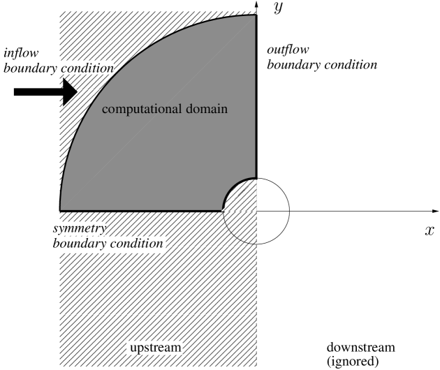
Figure 2: Plane flow around a cylinder: geometry and computational domain. By symmetry with respect to the horizontal axis, the computational domain is defined for the upper part only. The downstream flow is not simulated.

Our test is a 2D hypersonic plane flow of air–considered as a mixture of two vibrating gases, nitrogen and dioxygen–over a quarter of a cylinder which is supposed to be isothermal (see figure 2). Gas-solid wall interactions are modeled by the usual diffuse reflection. At the inlet, the flow is defined by the data given in table 1.

Mass concentration of $N_{2}$ ($c_{N_{2}}$)	$0.75$
Mass concentration of $O_{2}$ ($c_{O_{2}}$)	$0.25$
Mach number of the mixture	$10$
Velocity of the mixture	$2267m.s^{-1}$
Density of the mixture	$3.059\times 10^{-4}kg.m^{-3}$
Pressure of the mixture	$11.22Pa$
Temperature of the mixture	$127.6K$
Temperature of the cylinder	$293K$
Radius of the cylinder	$0.1m$

Table 1: Hypersonic flow around a cylinder: initial data

In this case, the vibrational energy is taken into account as described in section 3.1.2. The corresponding constitutive relations are obtained as explained in remark 4.1.

The flow conditions are such that molecules vibrate, but no chemical reactions are active (temperatures go up to $3000$K whereas chemical reactions occur at $5000$K at pressure $P=1$atm): our thermodynamical approach is reasonable. Since the test case is dense enough (the Knudsen number is around $0.01$) we can compare the new model with a Navier-Stokes code (a 2D finite volume code with structured meshes), in which are enforced the same viscosity and conductivity as in compressible Navier-Stokes asymptotics derived from the BGK model (see section 4.3). To validate the new model we have made four different simulations:

• a Navier-Stokes simulation without taking into account vibrations (called $NS1$),

• a Navier-Stokes simulation that takes into account vibrations (called $NS2$),

• a BGK simulation without taking into account vibrations (called $BGK1$),

• a BGK simulation that takes into account vibrations (called $BGK2$).

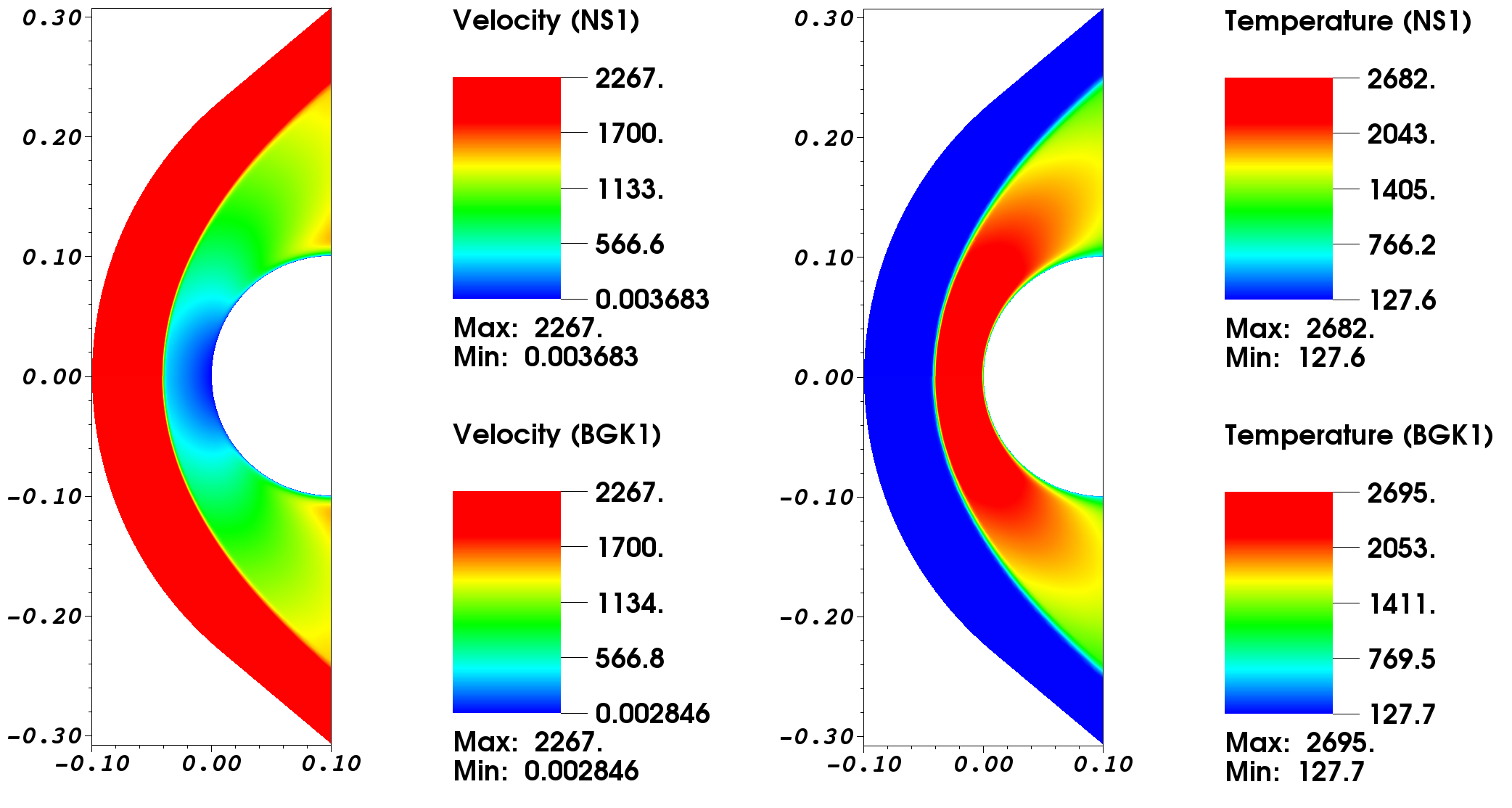
Figure 3: Non vibrating air: velocity and temperature fields (Top: NS1, bottom: BGK1)

The first comparison is between $NS1$ and $BGK1$, in order to show that the two model are consistent in this dense regimes, when there are no vibration energy. As it can be seen in figure 3, the results agree very well.

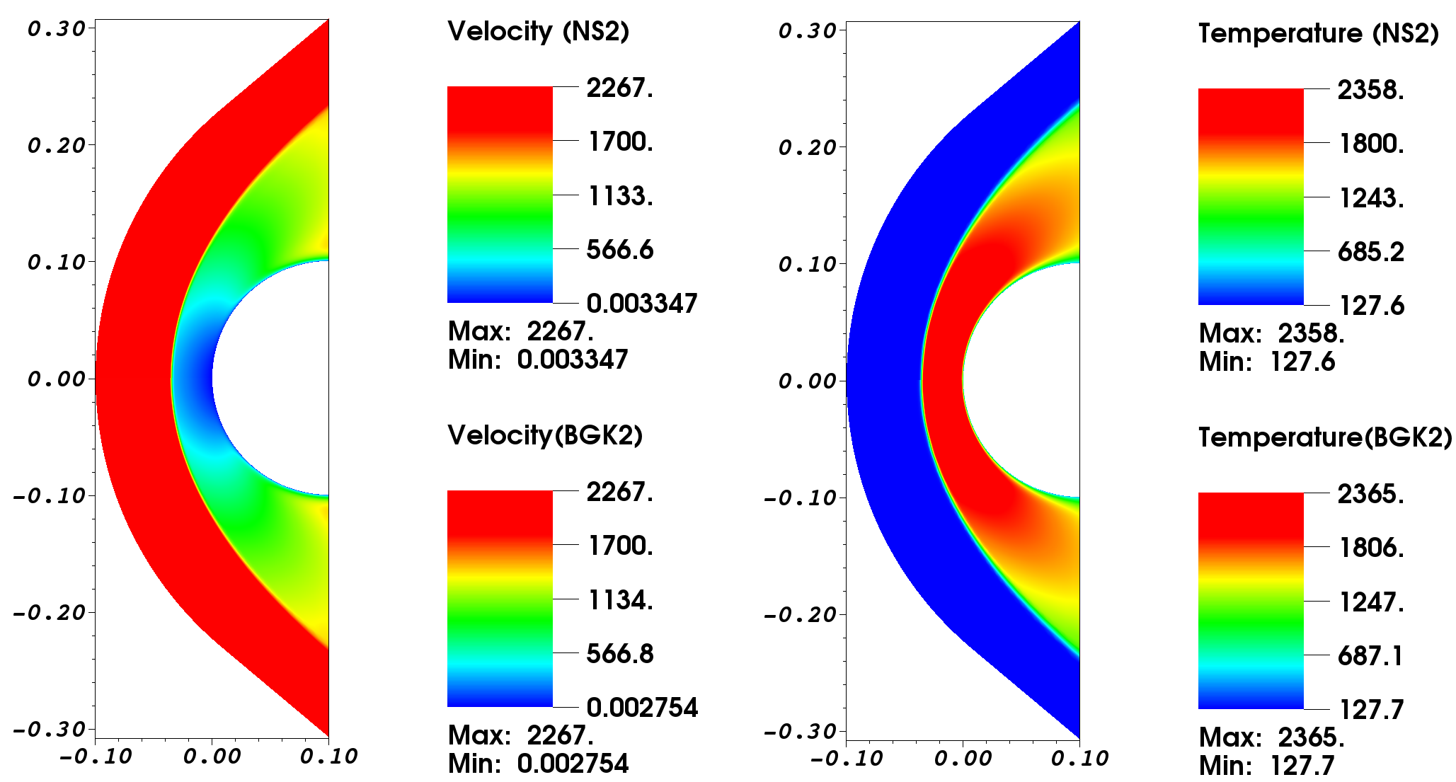
Figure 4: Vibrating air: velocity and temperature fields (Top: NS2, bottom: BGK2)

The second comparison is between $NS2$ and $BGK2$ to show we still have a good agreement when vibrations are taken into account. This is what we observe in figure 4. One can also observe that, due to vibrations, the temperature decreased from $2682K$ to $2358K$ for Navier-Stokes and from $2695K$ to $2365K$ for BGK.

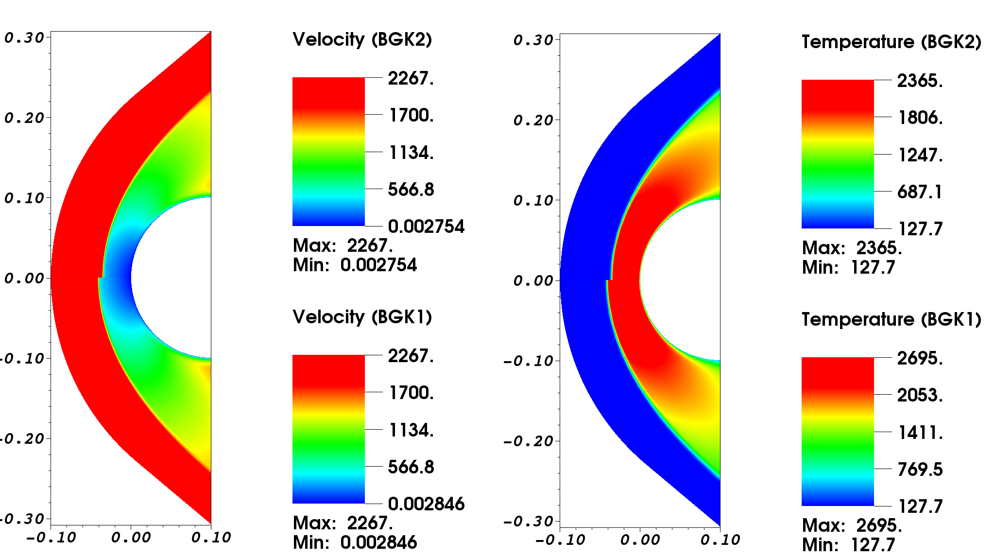
Figure 5: Vibrating and non-vibrating air: velocity field and temperature field (Top: BGK2, bottom: BGK1)

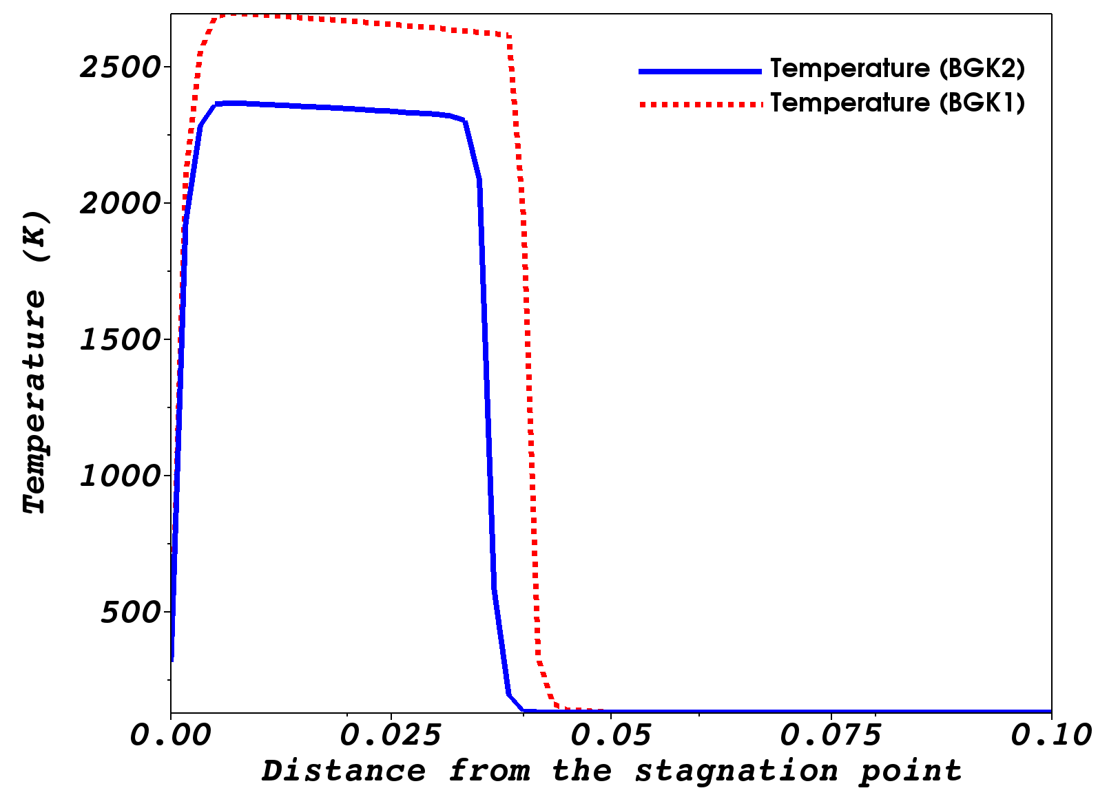
Figure 6: Vibrating and non-vibrating air: temperature profile along the stagnation line.

The last comparison is to show the influence of vibrational energy on the results. We compare $BGK1$ and $BGK2$, and we observe that the shock is not at the same position. Since there is a transfer of energy from translational and rotational modes to vibrational modes, the maximum temperature is lower and the shock is slightly close to the cylinder with BGK2 (see figure 5). We clearly see this difference with the temperature profile along the stagnation line, see figure 6.

To conclude this section, it can be said that when Navier-Stokes and BGK are set with the same viscosity and Prandtl number, results agree very well: but of course for more realistic test cases when the Prandtl number is not equal to one, there will be a discrepancy in the results that might be corrected with an ES-BGK extension of our model. This will be presented in a further work.

5.2 High temperature flow: reacting gas

In this section, we illustrate the ability of our model to account for chemical reactions in a high temperature flow. In order to simplify the analysis of our results, we consider here a single species flow of dioxygen. The geometry of the test case is the same as in the previous section, and the parameters of the upstream flow are the followings: the Mach number is $12$, the density is $10^{-3}$ kg.m^-3, so that the flow is in the near continuous regime (Kn$=4.29\times 10^{-4}$), the pressure is $33.15$ Pa, the temperature is $127.6$ K, and the temperature of the cylinder is still $283$ K.

In this case, the chemical reactions are taken into account with pressure and temperature laws as given by Hansen [16], both in our Navier-Stokes and BGK solvers. We obtain the comparison shown in figure 7 for the temperature field. The results given by both codes are very close. A closer look at the temperature profile along the stagnation line is also shown in figure 8: this profile shows that BGK results are excellent.

We are also able to obtain the concentration $c_{O}$ of monoatomic oxygen (see section 3.2), and this concentration is plotted in figure 9. Again both codes are in very good agreement, and these results show that there is dissociation of $O_{2}$ molecules in the largest temperature zones, since the concentration rises up to 12% there.

Finally, the importance of chemical reactions (dissociation) in this test case can be seen as follows. In figure 10, we compare the previous BGK results to a simulation made when vibrations are taken into account but the chemical reactions are not. This figure clearly shows that the non reacting BGK results are incorrect: the location of the shock is wrong, and the temperature is too high.

6 Conclusion

In this paper, we have proposed several generalized BGK models to account for high temperature effects (vibrations and chemical reactions). The first model is able to account for the fact that, for polyatomic gases, some internal degrees of freedom are partially excited with a level of excitation that depends on the temperature. In other words, we have derived a model for a polyatomic gas with a non-constant specific heat $c_{p}=c_{p}(T)$.

This model has been extended to take into account general constitutive laws for pressure and temperature, like in equilibrium chemically reacting gases in high temperature flows. By using a Chapman-Enskog analysis, we have derived compressible Navier-Stokes equations from this model that are consistent with these constitutive laws. This consistency has been illustrated on preliminary numerical tests, in which the importance to take vibration modes into account is clearly seen.

We point out that this new model can be reduced to a BGK system in which the molecular velocity is the only kinetic variable. This makes it possible to simulate a high temperature polyatomic gas for the cost of a simple monoatomic rarefied gas flow simulation.

The model for chemically reacting gases has been tested with a single species flow that shows its ability to account for dissociation, at least in the near continuum regime. Our model has still to be validated with comparisons to a full Boltzmann (DSMC) solver in the rarefied regime. It should also be extended to allow for various different time scales (viscous versus thermal diffusion time scale, translational versus rotational energy relaxation rates). This might be possible with the same approach as the one used to derive the ES-BGK model for polyatomic gases (see [3]).

Appendix A Gaussian integrals

We remind the definition of the absolute Maxwellian $M_{0}(V)=\frac{1}{(2\pi)^{\frac{3}{2}}}\exp(-\frac{|V|^{2}}{2})$. It is standard to derive the following integral relations (see [13], for instance), written with the Einstein notation:

$$\langle M_{0}\rangle_{V}=1,$$

$$\langle V_{i}V_{j}M_{0}\rangle_{V}=\delta_{ij},\qquad\langle V_{i}^{2}M_{0}\rangle_{V}=1,\qquad\langle|V|^{2}M_{0}\rangle_{V}=3,$$

$$\langle V_{i}^{2}V_{j}^{2}M_{0}\rangle_{V}=1+2\,\delta_{ij},\qquad\langle V_{i}V_{j}V_{k}V_{l}M_{0}\rangle_{V}=\delta_{ij}\delta_{kl}+\delta_{ik}\delta_{jl}+\delta_{il}\delta_{jk}$$

$$\langle V_{i}V_{j}|V|^{2}M_{0}\rangle_{V}=5\,\delta_{ij},\qquad\langle|V|^{4}M_{0}\rangle_{V}=15,$$

$$\langle V_{i}V_{j}|V|^{4}M_{0}\rangle_{V}=35\,\delta_{ij},\qquad\langle|V|^{6}M_{0}\rangle_{V}=105,$$

while all the integrals of odd power of $V$ are zero.

From the previous Gaussian integrals, it can be shown that for any $3\times 3$ matrix $C$, we have

$$\langle V_{i}V_{j}C_{kl}V_{k}V_{l}M_{0}\rangle_{V}=C_{ij}+C_{ji}+C_{ii}\delta_{ij}.$$

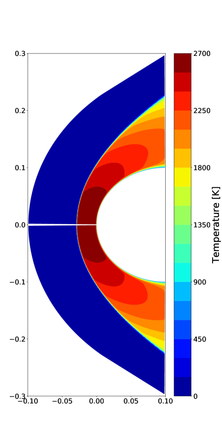
Figure 7: Dioxygen flow: temperature field obtained with a chemical equilibrium Navier-Stokes solver (top) and our chemical equilibrium BGK solver (bottom).

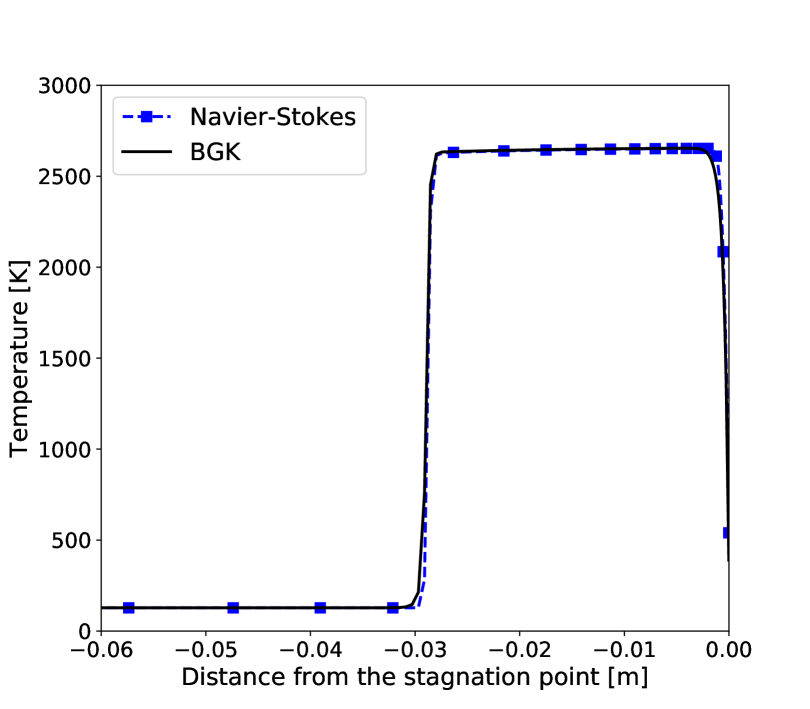
Figure 8: Dioxygen flow: temperature along the stagnation line.

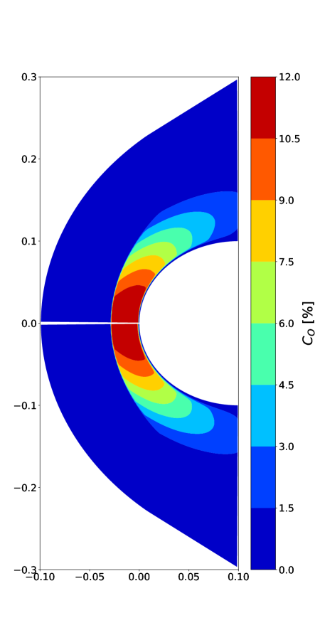
Figure 9: Dioxygen flow: concentration of monoatomic oxygen obtained with a chemical equilibrium Navier-Stokes solver (top) and our chemical equilibrium BGK solver (bottom).

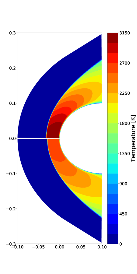
Figure 10: Dioxygen flow: temperature field obtained with our BGK solver with only vibrational energy (top), and our chemical equilibrium BGK solver (bottom).

References

- [1] J. Anderson. Hypersonic and High-Temperature Gas Dynamics, Second Edition. AIAA Education Series. American Institute of Aeronautics and Astronautics, 2006.
- [2] P. Andries, K. Aoki, and B. Perthame. A consistent BGK-type model for gas mixtures. Journal of Statistical Physics, 106(5):993–1018, Mar 2002.
- [3] P. Andries, P. Le Tallec, J.-P. Perlat, and B. Perthame. The Gaussian-BGK model of Boltzmann equation with small Prandtl number. Eur. J. Mech. B-Fluids, pages 813–830, 2000.
- [4] T. Arima, T. Ruggeri, and M. Sugiyama. Rational extended thermodynamics of a rarefied polyatomic gas with molecular relaxation processes. Phys. Rev. E, 96:042143, Oct 2017.
- [5] T. Arima, T. Ruggeri, and M. Sugiyama. Extended thermodynamics of rarefied polyatomic gases: 15-field theory incorporating relaxation processes of molecular rotation and vibration. Entropy, 20(4), 2018.
- [6] C. Baranger, J. Claudel, N. Hérouard, and L. Mieussens. Locally Refined Discrete Velocity Grids for Stationary Rarefied Flow Simulations. Journal of Computational Physics, 257:572–593, October 2013.
- [7] G. A. Bird. Molecular Gas Dynamics and the Direct Simulation of Gas Flows. Oxford Engineering Science Series, 2003.
- [8] M. Bisi and M. J. Cáceres. A BGK relaxation model for polyatomic gas mixtures. Commun. Math. Sci., 14(2):297–325, October 2016.
- [9] M. Bisi, T. Ruggeri, and G. Spiga. Dynamical pressure in a polyatomic gas: Interplay between kinetic theory and extended thermodynamics. Kinetic & Related Models, 11(1):71, 2018.
- [10] C. Borgnakke and P. S. Larsen. Statistical collision model for monte carlo simulation of polyatomic gas mixture. Journal of Computational Physics, 18(4):405 – 420, 1975.
- [11] J.-F. Bourgat, L. Desvillettes, P. Le Tallec, and B. Perthame. Microreversible collisions for polyatomic gases and Boltzmann’s theorem. European J. Mech. B Fluids, 13(2):237–254, 1994.
- [12] I. D. Boyd and T. E. Schwartzentruber. Nonequilibrium Gas Dynamics and Molecular Simulation. Cambridge Aerospace Series. Cambridge University Press, 2017.
- [13] S. Chapman and T. G. Cowling. The mathematical theory of non-uniform gases. Cambridge University Press, 1970.
- [14] L. Desvillettes, R. Monaco, and F. Salvarani. A kinetic model allowing to obtain the energy law of polytropic gases in the presence of chemical reactions. European Journal of Mechanics - B/Fluids, 24(2):219 – 236, 2005.
- [15] B. Dubroca and L. Mieussens. A conservative and entropic discrete-velocity model for rarefied polyatomic gases. ESAIM Proceedings, 10:127–139, CEMRACS 1999.
- [16] C. F. Hansen. Approximations for the thermodynamic and transport properties of high-temperature air. Nasa, 1960.
- [17] A. B. Huang and D. L. Hartley. Nonlinear rarefied couette flow with heat transfer. Phys. Fluids, 11(6):1321, 1968.
- [18] S. Kosuge, H.-W. Kuo, and K. Aoki. A kinetic model for a polyatomic gas with temperature-dependent specific heats and its application to shock-wave structure. Journal of Statistical Physics, 177(2):209–251, Oct 2019.
- [19] E. V. Kustova and G. P. Oblapenko. Reaction and internal energy relaxation rates in viscous thermochemically non-equilibrium gas flows. Physics of Fluids, 27(1):016102, 2015.
- [20] S. Liu, P. Yu, K. Xu, and C. Zhong. Unified gas-kinetic scheme for diatomic molecular simulations in all flow regimes. Journal of Computational Physics, 259:96 – 113, 2014.
- [21] J. Mathiaud. Models and methods for complex flows: application to atmospheric reentry and particle / fluid interactions. Habilitation à diriger des recherches, University of Bordeaux, June 2018.
- [22] J. Mathiaud and L. Mieussens. A Fokker–Planck model of the Boltzmann Equation with Correct Prandtl Number. Journal of Statistical Physics, 162(2):397–414, Jan 2016.
- [23] J. Mathiaud and L. Mieussens. A Fokker–Planck model of the Boltzmann Equation with Correct Prandtl Number for polyatomic gases. Journal of Statistical Physics, 168(5):1031–1055, Sep 2017.
- [24] J.L. Montagné, H.C. Yee, G.H. Klopfer, and M. Vinokur. Hypersonic Blunt Body Computations Including Real Gas Effects. NASA Technical Memorandum, 100074, march 1988.
- [25] W.-F. Ng, T.J. Benson, and W.G. Kunik. Real gas effects on the numerical simulation of a hypersonic inlet. Journal of Propulsion and Power, 2(4):381–382, 1986.
- [26] B. Rahimi and H. Struchtrup. Macroscopic and kinetic modelling of rarefied polyatomic gases. Journal of Fluid Mechanics, 806:437–505, 2016.
- [27] Henning Struchtrup. Macroscopic transport equations for rarefied gas flows. Interaction of Mechanics and Mathematics. Springer, Berlin, 2005. Approximation methods in kinetic theory.