Fluctuations of gravitational waves in Eddington inspired Born-Infeld theory

Abstract

In this paper we review the EiBI gravity in the presence of a cosmological constant and its tensor perturbations analysis. We show the existence of gravitational waves in the past-time, seeing as a result the smooth transition between high-energy densities (where the EBI dynamics plays its role) and low-energy densities (GR). We obtain the fluctuation spectrum for the graviton in this theory, where for small values of $k$ the fluctuations are strongly suppressed and for large values of $k$ these fluctuations vanish during the De Sitter expansion.

I Introduction

One of the greatest jigsaws in the current physics research is to understand the nature of dark energy and dark matter Zhao:2017cud ; Copeland:2006wr ; Bird:2016dcv ; Clowe:2006eq . Currently, dark energy is one of the main classes of models to describe the cosmic late-time acceleration, which has been confirmed by a large number of observations such as measurements SNIa Riess:1998cb-Perlmutter:1998np , BAO Eisenstein:2005su , CMBR anisotropies Spergel:2003cb , LSS Tegmark:2003ud and WL Jain:2003tba . Future projects and surveys surveys are underway to discover the underlying cause of this phenomena. Recently, the first multimessenger gravitational-wave (GW) observation of a binary neutron star made by LIGO-Virgo detector network set a way to infer cosmological parameters independently of the cosmic distance ladder TheLIGOScientific:2017qsa , getting a better value for the Hubble constant – and by extension, a better understanding of dark energy – could be right on the horizon.

In the light of rich observed data, either we just know some properties of each component of the dark sector or one might have a new proposal of the gravitational theory without the need of these dark components instead. Some attempts has been done in order to achieve these issues, e.g in Banados:2008fi was presented a class of bigravity with solutions that can be interpolate between matter and acceleration epochs. In Banados:2008fj ; Banados:2010ix was presented a non-conventional formulation in terms of the affine connection $\Gamma^{\mu}_{\alpha\beta}$ and a space-time metric $g_{\alpha\beta}$ such that the gravitational action is given by:

$$S_{EiBI}[g,\Gamma,\Psi] = \frac{2}{\kappa}\int{d^{4}x\left[\sqrt{\left|g_{\mu\nu}+\kappa R_{\mu\nu}(\Gamma)\right|}-\lambda\sqrt{g}\right]}$$ (1)

$$+S_{m}[g,\Psi],$$

where $\kappa=8\pi G$, $\Psi$ denotes any additional matter fields, $R_{\mu\nu}$ is the symmetric Ricci tensor constructed with $\Gamma$. The term insight the root denote the determinant. Here the matter is added in the usual way. The connection between (1) and cosmological observations has been done in Scargill:2012kg . Despite its preliminaries success, in bouncing cosmological solutions cases it has already been observed that EiBI suffers from instabilities associated with the growth of tensor perturbations EscamillaRivera:2012vz . In latest works, further considerations about the tensor perturbations in EiBI were made Avelino:2012ue ; BeltranJimenez:2017uwv ; BeltranJimenez:2017doy ; Jana:2017ost . Moreover, the aim of this paper is to take a step forward in order to calculate the fluctuations of the EiBI tensor perturbations and compute the graviton mass at two limits: for low-energy densities (General Relativity -GR-) and high-energy densities (Eddington limit).

This paper is organised as follows: In Sec. II we will review the field equations for the EiBI theory. In Sec. III we summarise the limits in this theory. In Sec. IV we calculate the GW equation for the EiBI theory and it will be thoroughly discussed. Also, as a main goal of this paper, we compute the evolution of the graviton mass at both, high and low densities. In Sec. V we explore the fluctuation spectrum in this theory.

II EiBI field equations

From (1) we can calculate the Einstein field equations by varying with respect to the metric $g_{\mu\nu}$ and the variation with respect to the connection fixes the affine connection to be $\Gamma$:

$$\sqrt{\left|\frac{q}{g}\right|}(q^{-1})^{\mu\nu}-\lambda g^{\mu\nu}=-\kappa T^{\mu\nu},$$ (2)

$$\nabla_{\alpha}\left[\sqrt{q}(q^{-1})^{\mu\nu}\right]-\nabla_{\beta}\left\{\sqrt{q}\left[\delta^{\mu}_{\alpha}(q^{-1})^{\beta\nu}+\delta^{\nu}_{\alpha}(q^{-1})^{\beta\mu}\right]\right\}=0,$$

$$q_{\mu\nu}=g_{\mu\nu}+\kappa R_{\mu\nu},$$ (3)

where $\lambda=1+\kappa\Lambda$, and $\kappa$ is a constant with the inverse dimensions of $\Lambda$. Notice that these field equations are obtained from independent variation of the metric and $\Gamma$. The auxiliary tensor $q_{\mu\nu}$ is not the space-time metric and $\lambda$ can be related to the cosmological constant term from a GR point of view.

III Limits in the EiBI theory

Focusing on the dynamics of homogeneous and isotropic metric in (2)-(3), we consider a line element with time and spatial components for each metric:

$$g^{00} = 1,\hskip 22.76228ptg^{ij}=a^{-2}\delta^{ij},$$

$$q^{00} = X^{-2},\quad q^{ij}=(aY)^{-2}\delta^{ij},$$ (4)

Eqs. (2)-(II) can be solved analytically using (III) to derive the conventional Friedmann cosmology at late-times. The zero-component evolution equation with $\sqrt{|q/g|}=|XY^{3}|$ is:

$$3\kappa\left(H+\frac{\dot{Y}}{Y}\right)^{2}=X^{2}\left(1-\frac{3}{2Y^{2}}\right)+\frac{1}{2},$$ (5)

where

$$|X| = \frac{(1+\kappa P_{T})^{2}}{[(1+\kappa\rho_{T})(1-\kappa P_{T})^{1/4}]},$$ (6)

$$|Y| = [(1+\kappa\rho_{T})(1-\kappa P_{T})^{1/4}],$$ (7)

with $\rho_{T}=\rho+\Lambda$ and $P_{T}=P-\Lambda$. Let us assume radiation domination as: $\rho_{T}=\rho$ and $P_{T}=P=\rho/3$, we find that $X$ and $Y$ at late times behaves as:

$$|X| \simeq 1-\frac{5}{6}\kappa\rho+O(\kappa^{2}),$$ (8)

$$|Y| \simeq a+\frac{a}{6}\kappa\rho+O(\kappa^{2}).$$ (9)

If $X=Y=1$ the latter reduces to the low-energy densities limit (GR limit). Now, considering high energy densities (Eddington limit) $\rho\rightarrow\rho_{B}$, where the subindex $B$ indicates the existence of a minimum value for the scale factor Banados:2010ix then the approximation for the variables $X$ and $Y$ are

$$|X| = \frac{\left(1-\frac{\bar{\rho}}{3}\right)^{2}}{[(1+\bar{\rho})\left(1-\frac{\bar{\rho}}{3}\right)]^{1/4}},$$ (10)

$$|Y| = [(1+\bar{\rho})\left(1-\frac{\bar{\rho}}{3}\right)]^{1/4},$$ (11)

where we introduce $\bar{\rho}=\kappa\rho$. We see a critical point at $\bar{\rho}=\rho_{B}=3$. Rewriting (5) we obtain

$$3H^{2} = \frac{1}{\kappa}\left[\bar{\rho}-1+\frac{1}{3\sqrt{3}}\sqrt{(\bar{\rho}+1)(3-\bar{\rho})^{3}}\right]$$ (12)

$$\times\left[\frac{(1+\bar{\rho})(3-\bar{\rho})^{2}}{(3+\bar{\rho}^{2})^{2}}\right],$$

where for $\bar{\rho}\ll 1$ we have $H^{2}\simeq\rho/3$. Eq.(12) has critical points for $H(\rho_{B})=0$ in a maximum density $\rho_{B}=0,-1,3$. Each critical point appear when $Y^{2}=3X^{2}/(2X^{2}+1)$. Notice that each critical density has an analytical solution that corresponds to an expansion of the scale factor depending of the sign of $\kappa$ (see Figure 1):

• When $\bar{\rho}$ ($\kappa\approx 1$), $X=Y=1$, then we have a minimum scale factor at $\dot{a}=0$ and the universe its stationary and has a minimum size $a=a_{B}\approx 10^{-32}(\kappa)^{1/4}a_{0}$, where $a_{0}$ is the scale factor today. This replace the usual Big Bang singularity of Einstein’s model by a cosmic bounce.

• When $\bar{\rho}=3(\kappa>0)$, $X=Y=0$ and the solution is exponential-like $(a/a_{B})-1\propto e^{t-t_{B}}$, which corresponds to a loitering solution.

• When $\bar{\rho}=1$ ($\kappa<0$), $X=(3\cdot 4^{3})^{1/4}/9$ and $Y=(4^{3})^{1/4}$, with solution $(a-a_{B})\propto|t-t_{B}|^{2}$, which corresponds to a bouncing solution.

Given that the solution for the radiation is $\rho=\rho_{0}/a^{4}=\rho_{0}/(a_{B}+\delta a)^{4}$, we can expand the density around the small variation of $a$ ($\delta a$),

$$\rho \propto \frac{\rho}{a^{4}_{B}}+4\rho_{0}\frac{\delta a}{a^{5}_{B}}+O(\delta a^{2}),$$ (13)

$$\rho \propto \rho_{B}+4\rho_{B}\frac{\delta a}{a_{B}}+O(\delta a^{2}),$$ (14)

where $\rho_{B}=\rho_{0}a^{-4}_{B}$ is the maximum density. As $a=a_{B}+\delta a$ then $(a/a_{B})-1=\delta a/a_{B}$,

$$\rho \propto \rho_{B}+4\rho_{B}\left(\frac{a}{a_{B}}-1\right)+O\left[a^{2}_{B}\left(\frac{a}{a_{B}}-1\right)^{2}\right],$$

$$a \propto 1+(t-t_{B})+O[(t-t_{B})^{2}].$$ (15)

At early times (III) shows a universe with a maximum density and constant scale factor.

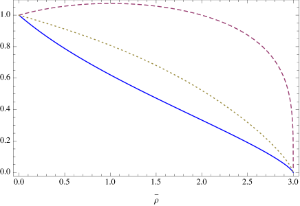
Figure 1: The evolution of $X$ (blue solid line) and $Y$ (purple dashed line) from the low-energy to high-energy density limit. We observe two critical points for each limit at $\rho\rightarrow\rho_{B}=0$ and $\rho\rightarrow\rho_{B}=3/\kappa$, respectively. The yellow-dotted curve represents the evolution of $Y^{2}=\frac{3X^{2}}{2X^{2}+1}$ that gives $H^{2}=0$.

IV EiBI tensor perturbations

We can consider a perturbed homogeneous and isotropic spacetime by choosing the two metrics to be of the form:

$$g^{00} = 1,\hskip 22.76228ptg^{ij}=a^{-2}(\delta^{ij}-h^{ij}),$$

$$q^{00} = X^{-2},\quad q^{ij}=(aY)^{-2}(\delta^{ij}-\gamma^{ij}),$$ (16)

where $h_{ij}$ and $\gamma_{ij}$ are traceless and transverse, i.e $\partial_{i}h^{ij}=\partial_{i}\gamma^{ij}=0$, $h_{ii}=\gamma_{ii}=0$, respectively. To construct the perturbed field equations we compute the quantities:

$$(q^{-1})^{ij} = (aY)^{-2}(\delta^{ij}-\gamma^{ij}),$$ (17)

$$(g)^{ij} = a^{2}(\delta^{ij}-h^{ij}),$$ (18)

$$\delta T^{ij} = -Pa^{-2}h^{ij},$$ (19)

where we take $T_{\mu\nu}=(\rho+P)u_{\mu}u_{\nu}+Pg_{\mu\nu}$ with $u^{\mu}=(1,0,0,0)$.

An interesting results derived from the field equations is that $\gamma_{ij}=h_{ij}$, i.e it was found in EscamillaRivera:2012vz that $\gamma_{ij}$ is completely locked to the behaviour of $h_{ij}$. After following this consideration we can write the evolution equation for $h_{ij}$ as

$$h^{\prime\prime}_{ij}+\left(4\frac{(aY)^{\prime}}{(aY)}-2\frac{a^{\prime}}{a}\right)h^{\prime}_{ij}+\left[\frac{X^{\prime\prime}}{X}+2\frac{X^{\prime}}{X}\frac{(aY)^{\prime}}{(aY)}+\frac{(aY)^{\prime\prime}}{(aY)}\right.$$

$$\left.-4\frac{X^{\prime}}{X^{2}}\frac{(aY)^{\prime}}{(aY)}\frac{a^{\prime}}{a}+2\frac{a^{\prime 2}}{a^{2}}-\frac{a^{\prime\prime}}{a}-2\frac{(aY)^{\prime 2}}{(aY)^{2}}-2\frac{X^{\prime 2}}{X^{2}}\right.$$

$$\left.-2k^{2}\frac{X^{\prime}}{X}\frac{(aY)^{\prime}}{(aY)}+k^{2}+\frac{X(aY)^{3}+a^{3}\lambda}{\kappa\lambda aX^{2}(aY)^{2}}\right]h_{ij}=0.$$ (20)

where the prime denotes derivatives w.r.t the conformal time $\eta$. This graviton equation can be rewriten by using $|aY|$ and the component $R_{00}$ to obtain

$$\left[\kappa\sqrt{-(\kappa\rho+1)(\kappa\rho-3)^{3}}(\kappa\rho+1)(\kappa^{2}\rho^{2}+3)\right]h^{\prime\prime}_{ij}$$

$$+\left[-\frac{2}{9}\sqrt{3}\kappa a(\kappa\rho-1)(\kappa\rho-3)\sqrt{-(\kappa\rho)(\kappa\rho-3)^{3}}\right.$$

$$\left.\sqrt{(9\kappa\rho+\sqrt{3}\sqrt{(\kappa\rho+1)(\kappa\rho-3)^{3}}-9)(\kappa\rho+1)}\right]h^{\prime}_{ij}$$

$$+\{(\kappa^{2}\rho^{2}+3)\sqrt{-(\kappa\rho+1)(\kappa\rho-3)^{3}}\left[\frac{2}{3}a^{2}\right.$$

$$\left.\sqrt{-(\kappa\rho+1)(\kappa\rho-3)^{3}}+k^{2}\kappa(\kappa\rho-3)\right]$$

$$+\frac{2\sqrt{3}}{3}(\kappa\rho+1)(\kappa\rho-3)^{3}\}h_{ij}=0.$$ (21)

At low-energy densities, if we expand the r.h.s of (IV) we obtain

$$\frac{1}{\sqrt{3}}\left(2\sqrt{\rho}h^{\prime}_{ij}+\sqrt{3}k^{2}h_{ij}\right)+4\left(\sqrt{3}\rho^{3/2}h^{\prime}_{ij}+\frac{k^{2}}{3}\rho h_{ij}\right)\kappa$$

$$+O(\kappa^{2})\approx 0,$$ (22)

where at late times $(\kappa\ll 1)$ and using $3H^{2}=\rho$ we recover the Helmholtz equation.

At high-energy densities, (IV) has a critical point $\rho_{B}=3/\kappa$, therefore

$$h^{\prime\prime}_{ij}=0\quad\rightarrow\quad h_{ij}\approx h_{0}\eta,$$ (23)

then $h_{ij}$ grows linearly at early times for

$${\lim_{\bar{\rho}\to 3}}\left[\kappa\sqrt{-(\kappa\rho+1)(\kappa\rho-3)^{3}}(\kappa\rho+1)(\kappa^{2}\rho^{2}+3)\right]=0.$$ (24)

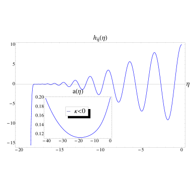
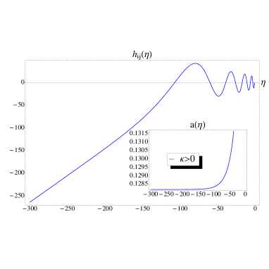
Figure 2: Numerical solutions for (IV) in conformal time. The footnote plots (inside) show the evolution of the scale factor for both values of $\kappa$.

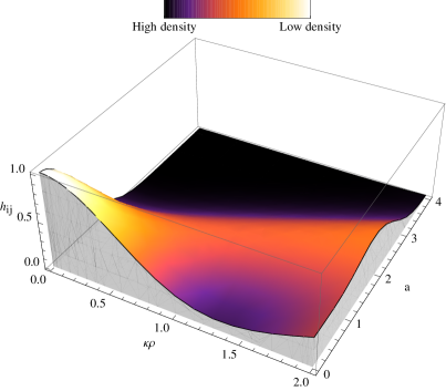
Figure 3: Numerical solution for (IV). We notice the transition between low-energy and high energy densities.

Performing the numerical integration of (IV)-(IV) we see the predicted behaviour (Figure 2): From the evolution of the scale factor we notice the smooth transition between high-energy densities (where the EBI dynamics plays its role) and low-energy densities (GR) (Figure 3). From the solution $h_{ij}$, we notice the linear grow of the GW (23) and as time evolves we have the damped oscillations in the GR limit.

IV.1 Graviton mass

Consider the field equations

$$R^{\mu\nu}-\frac{1}{2}g^{\mu\nu}R=-\kappa(T^{\mu\nu}+T^{\mu\nu}_{\text{mass}}),$$ (25)

where usually the extra term $T^{\mu\nu}_{\text{mass}}$ depends of the graviton mass $m_{g}$ and the background metric

$$T^{\mu\nu}_{\text{mass}} = -m_{g}\left\{(g^{-1}_{0})^{\mu\sigma}\left[(g-g_{0})_{\sigma\rho}-\frac{1}{2}(g_{0})_{\sigma\rho}(g_{0})^{\alpha\beta}\right.\right.$$ (26)

$$\left.\left.(g-g_{0})_{\alpha\beta}\right]((g_{0})^{-1})^{\rho\nu}\right\},$$

where if $m_{g}\rightarrow 0$ we recover the usual Einstein field equations. If we consider the background metric with a small perturbation to obtain for this mass term:

$$T^{\mu\nu}_{\text{mass}}=-m_{g}\left\{h_{\mu\nu}-\frac{1}{2}\left[((g_{0})^{-1})^{\alpha\beta}h_{\alpha\beta}\right](g_{0})_{\mu\nu}\right\},$$ (27)

where, for $\delta T_{\mu\nu}=0$, $\delta G_{\mu\nu}=-\kappa\delta T^{\text{mass}}_{\mu\nu}$, we can rewrite the perturbed equation as:

$$h^{\prime\prime}_{ij}+2Hh^{\prime}_{ij}+(k^{2}+m^{2}_{g})h_{ij}=0.$$ (28)

This equation is similar to the equation for a free massive scalar field in a flat FRW background. Now, from the perturbation of (3) $\kappa\delta R_{ij}=\delta q_{ij}-\delta g_{ij}$ we obtain:

$$\delta R_{ij}+\frac{a^{2}}{\kappa}\left(\frac{XY^{3}}{\lambda}+1\right)h_{ij}=0.$$ (29)

If we compare the latter with (28) we obtain

$$m^{2}_{g}=\frac{1}{\kappa}\left[\frac{(1+\kappa\rho_{T})(1-\kappa P_{T})^{3}}{1+\kappa\Lambda}+1\right],$$ (30)

which is the graviton mass that takes the following values:

• $\frac{XY^{3}}{\lambda}<-1$ gives a large tachyonic mass $m^{2}_{g}<0$ implying the unstable evolution of tensor perturbations,

• $\frac{XY^{3}}{\lambda}>-1$, the growth of the tensor perturbations is suppressed.

Eq. (28) reduces to

$$h^{\prime\prime}_{ij}+2Hh^{\prime}_{ij}+k^{2}h_{ij}=0,\quad\text{for}\quad p^{2}\gg m^{2}_{g},$$ (31)

and

$$h^{\prime\prime}_{ij}+2Hh^{\prime}_{ij}+m^{2}_{g}=0,\quad p^{2}\ll m^{2}_{g},\rightarrow\lambda\left(\frac{\kappa k^{2}}{a^{2}}-1\right)\ll XY^{3},$$ (32)

where $p^{2}\equiv a^{-2}k^{2}$ is the physical momentum.

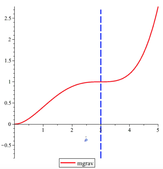
Figure 4: Evolution of the graviton mass in terms of $\bar{\rho}$. The dashed-blue line divide the high-energy density limit (right side) and low-energy density limit (left side). The critical point is located at $\bar{\rho}=3/\kappa$ for $|\kappa|=1$.

At high-energy densities ($\kappa\rho\rightarrow 3$) and in radiation regime (Figure 4)

$$m^{2}_{g_{\text{rad}}}\propto\frac{1}{\kappa}\left[(1+\bar{\rho})\left(1-\frac{1}{3}\bar{\rho}\right)+1\right]=\frac{1}{\kappa}.$$ (33)

When $m_{g}>1$ there is a growth of the tensor perturbations, after the graviton crosses the critical point $\bar{\rho}=3/\kappa$ at low-energy density ($0<m_{g}<1$) the growth is suppressed.

V Fluctuations in GW EiBI

We rewrite the graviton equation (IV) as:

$$h^{\prime\prime}_{ij}+Fh^{\prime}_{ij}+(G+Jk^{2})h_{ij}=0,$$ (34)

where

$$F=2\left[2\frac{(aY)^{\prime}}{(aY)}-\frac{a^{\prime}}{a}\right],$$ (35)

$$G = \frac{X^{\prime\prime}}{X}+2\left(\frac{X^{\prime}}{X}\right)\left[\frac{(aY)^{\prime}}{(aY)}\right]+\frac{(aY)^{\prime\prime}}{(aY)}$$ (36)

$$-4\left(\frac{X^{\prime}}{X^{2}}\right)\left[\frac{(aY)^{\prime}}{(aY)}\right]\left(\frac{a^{\prime}}{a}\right)+2\left(\frac{a^{\prime}}{a}\right)^{2}$$

$$-\frac{a^{\prime\prime}}{a}-2\left(\frac{X^{\prime}}{X}\right)^{2}-2\left[\frac{(aY)^{\prime}}{(aY)}\right]^{2}+\xi,$$

$$J=1-2\left(\frac{X^{\prime}}{X}\right)\left[\frac{(aY)^{\prime}}{(aY)}\right],$$ (37)

$$\xi=\frac{X(aY)^{3}+a^{3}\lambda}{\kappa\lambda aX^{2}(aY)^{2}}.$$ (38)

We use the change of variable $u=zh$ to avoid the friction-type term. We have at low-energy densities:

$$u^{\prime\prime}+\left(-\frac{z^{\prime\prime}}{z}+k^{2}\right)u=0,$$ (39)

and at high-energy densities:

$$u^{\prime\prime}+\left(-\frac{z^{\prime\prime}}{z}+G+Jk^{2}\right)u=0,$$ (40)

For each Fourier mode $k$ the above equations are the harmonic oscillator with time-dependent frequency

$$\omega_{k} := \sqrt{k^{2}-\frac{z^{\prime\prime}}{z}},$$ (41)

$$\omega_{k} := \sqrt{G+Jk^{2}-\frac{z^{\prime\prime}}{z}}.$$ (42)

If the expansion is rapid enough, $\omega_{k}$ becomes imaginary.

Will use the following definition for the quantum fluctuations where $g_{B}$ is an observable with mean value

$$g_{B}=<\Omega|g_{B}|\Omega>=<0|Aa+Ba^{{\dagger}}|0>=0,$$ (43)

and the variance is

$$[\delta g_{B}]^{2}=<\Omega|{g_{B}}^{2}|\Omega>\approx a^{-2}k^{3}|u_{k}|^{2}.$$ (44)

We define the fluctuation spectrum as the standard deviation as a function of $k$

$$\delta g_{k}:=a^{-1}k^{3/2}|u_{k}|.$$ (45)

V.1 Solutions of Eq.(39)

• Case 1. Minkowski spacetime $z=1$. Solving (39) and using (41)-(45), the solutions for the mode function and the fluctuation spectrum are

  $$u_{k,\eta} = (1/\sqrt{k})e^{i\eta k},$$

  $$\delta g_{k} = k^{3/2}/\sqrt{k}=k^{3}.$$ (46)

  We observed that at small $k$ (large scale), the fluctuations are strongly suppressed. Analogous to the numerical solutions, when the scale factor is constant we observed a fast growing of the graviton mode $h_{ij}$.

• Case 2. De Sitter spacetime. We consider $z=e^{\alpha t}=-(\alpha\eta)^{-1},$ with $\eta(t)=\int{z(t^{\prime})^{-1}dt^{\prime}}$. The frequency is

  $$\omega_{k,\eta}=k^{2}-\frac{2}{\eta^{2}}.$$ (47)

  The modes $k$ oscillate if $|\eta|\gg\sqrt{2}/k$ and the $\omega$ is an imaginary quantity when $|\eta|\ll\sqrt{2}/k$. The solutions are

  $$u_{k,\eta} = -\sqrt{\frac{2}{\pi k^{3}}}\left[(C_{1}k\eta+C_{2})\cos{(k\eta)}\right.$$ (48)

  $$\left.-(-C_{1}+C_{2}k\eta)\sin{(k\eta)}\right],$$

  and

  $$\delta g_{k,\eta} = -\alpha\eta\sqrt{\frac{2}{\pi}}\left[(C_{1}k\eta+C_{2})\cos{(k\eta)}\right.$$ (49)

  $$\left.-(-C_{1}+C_{2}k\eta)\sin{(k\eta)}\right],$$

  with $C_{1}$ and $C_{2}$ constants of integration. Notice that as $t\rightarrow-\infty$ we have $\eta\rightarrow-\infty$, but as $t\rightarrow\infty$ we have $\eta\rightarrow 0$. At large $k$ we have the usual fluctuation spectrum for Minkowski spacetime. As $t\rightarrow\infty$, the fluctuations vanishes during the De Sitter expansion.

V.2 Solutions for Eq.(40)

For (40) is not so simple to consider the same assumptions as the latter case since there is a dependence of $X$ and $aY$ in $G$ and $J$. Therefore, let us consider an expansion over $1/\eta$. We can rewrite the expressions for $X$ and $Y$ as:

$$|Y| = [(1+\kappa\rho_{T})(1-\kappa P_{T})^{1/4}],$$ (50)

$$|X| = \frac{(1+\kappa P_{T})^{2}}{|Y|},$$ (51)

where with $\rho=r_{0}-\frac{\lambda}{\kappa}$. The expressions for the total density and pressure are

$$P_{T} = \frac{1}{\kappa}(1-\lambda\pi_{0})-\pi_{0}\rho=-\frac{1}{\kappa}\pi_{0}r_{0},$$ (52)

$$\rho_{T} = r_{0}-\frac{1}{\kappa},$$ (53)

and now

$$|X| = \frac{1-\pi_{0}r_{0}}{\kappa r_{0}(1+\pi_{0}r_{0})^{1/4}},$$ (54)

$$|Y| = \kappa r_{0}(1+\pi_{0}r_{0})^{1/4}.$$ (55)

In the asymptotic past these expansions are reduced to $p_{1}=\pi_{0}$ and $\rho_{1}=r_{0}$. We rewrite (40) for the ER as:

$$u^{\prime\prime}+\left(-\frac{z^{\prime\prime}}{z}+\xi_{0}+k^{2}\right)u=0,$$ (56)

where

$$\xi_{0}=\frac{(1-\pi_{0}r_{0})(1+\pi_{0}r_{0})^{1/2}-\lambda\kappa r_{0}}{\kappa r_{0}\left[\kappa\lambda(1-\pi_{0}r_{0})(1+\pi_{0}r_{0})^{1/4}\right]}.$$ (57)

For the Minkowski case, we obtain similar solutions as in (• ‣ V.1) but with an extra constant term $\xi_{0}$ in the exponential. For the DeSitter case also we obtain oscillating solution, but the harmonic functions will be weighted by a $(\sqrt{\xi_{0}}+k)$ term. When $\pi_{0},r_{0}\ll 1$ there is an increase on the amplitude of the fluctuation spectrum. In Figure 5 we show the power spectrum of the graviton equation ($P_{g}\propto|\delta g_{k}|^{2}$).

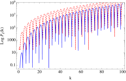
Figure 5: Power spectrum for the GW (40) using the fluctuations (49). The blue-solid curve represent a value of $\xi_{0}=99$ and the red-dashed curve for $\xi_{0}=0.003$.

VI Conclusions

The EiBI theory has been a successful proposal for modify gravity theories, in which it is replaced the usual Big Bang singularity of Einstein’s model by a cosmic bounce. Also, it was observed that this proposal suffers from a tensor instability. In regards to this, here we have discussed the evolution of the EiBI-GW equation. Furthermore, we obtain the value for the graviton mass in EiBI gravity at high and low energy densities, where for $k\ll 1$ the fluctuations are strongly suppressed and for $k\gg 1$ these ones vanish during the De Sitter expansion.

Work still needs to be done before compare with current observations. Although within this paper, we review the importance of use the EiBI theory in future test of GW.

- (1) G. B. Zhao et al., Nat. Astron. 1 (2017) 627 doi:10.1038/s41550-017-0216-z [arXiv:1701.08165 [astro-ph.CO]].
- (2) E. J. Copeland, M. Sami and S. Tsujikawa, Int. J. Mod. Phys. D 15, 1753 (2006) [arXiv:hep-th/0603057].
- (3) S. Bird, I. Cholis, J. B. Mu oz, Y. Ali-Ha moud, M. Kamionkowski, E. D. Kovetz, A. Raccanelli and A. G. Riess, Phys. Rev. Lett. 116 (2016) no.20, 201301 doi:10.1103/PhysRevLett.116.201301
- (4) D. Clowe, M. Bradac, A. H. Gonzalez, M. Markevitch, S. W. Randall, C. Jones and D. Zaritsky, Astrophys. J. 648, L109 (2006) [arXiv:astro-ph/0608407].
- (5) A. G. Riess et al. [Supernova Search Team Collaboration], Astron. J. 116, 1009 1998 [astro-ph/9805201]. S. Perlmutter et al. [Supernova Cosmology Project Collaboration], Astrophys. J. 517, 565 1999 Available online: [astro-ph/9812133].
- (6) D. J. Eisenstein et al. [SDSS Collaboration], Astrophys. J. 633, 560 2005 Available online: [astro-ph/0501171].
- (7) D. N. Spergel et al. [WMAP Collaboration], Astrophys. J. Suppl. 148, 175 2003 Available online: [astro-ph/0302209].
- (8) M. Tegmark et al. [SDSS Collaboration], Phys. Rev. D 69, 103501 2004 Available online: [astro-ph/0310723].
- (9) B. Jain and A. Taylor, Phys. Rev. Lett. 91, 141302 2003 Available online: [astro-ph/0306046].
- (10) R. Laureijs et al. [EUCLID Collaboration], ESA/SRE 201112 Available online: arXiv:1110.3193 [astro-ph.CO]. L. Amendola et al. [Euclid Theory Working Group Collaboration], Living Rev. Rel. 16, 6 2013 Available online: [arXiv:1206.1225 [astro-ph.CO]]. L. Samushia et al., Mon. Not. Roy. Astron. Soc. 439, no. 4, 3504 2014 Available online: [arXiv:1312.4899 [astro-ph.CO]]. F. Abdalla et al., FERMILAB-TM-2547-AE 2012 Available online: arXiv:1209.2451 [astro-ph.CO]. Myers, S. T., Abdalla, F. B., Blake, C., Koopmans, L., Lazio, J., and Rawling, S. 2009, Vol. 2010, Astro2010: The Astronomy and Astrophysics Decadal Survey, 219, Available online: [arXiv:0903.0615].
- (11) B. P. Abbott et al. [LIGO Scientific and Virgo Collaborations], Phys. Rev. Lett. 119, no. 16, 161101 (2017) doi:10.1103/PhysRevLett.119.161101 [arXiv:1710.05832 [gr-qc]].
- (12) M. Banados, A. Gomberoff, D. C. Rodrigues and C. Skordis, Phys. Rev. D 79, 063515 (2009) [arXiv:0811.1270 [gr-qc]].
- (13) M. Banados, P. G. Ferreira and C. Skordis, Phys. Rev. D 79, 063511 (2009) [arXiv:0811.1272 [astro-ph]].
- (14) M. Banados, P. G. Ferreira, Phys. Rev. Lett. 105, 011101 (2010). [arXiv:1006.1769 [astro-ph.CO]].
- (15) J. H. C. Scargill, M. Banados and P. G. Ferreira, Phys. Rev. D 86, 103533 (2012) doi:10.1103/PhysRevD.86.103533 [arXiv:1210.1521 [astro-ph.CO]]. A. De Felice, B. Gumjudpai and S. Jhingan, Phys. Rev. D 86, 043525 (2012) doi:10.1103/PhysRevD.86.043525 P. P. Avelino, Phys. Rev. D 85, 104053 (2012) doi:10.1103/PhysRevD.85.104053 [arXiv:1201.2544 [astro-ph.CO]].
- (16) C. Escamilla-Rivera, M. Banados and P. G. Ferreira, Phys. Rev. D 85, 087302 (2012) doi:10.1103/PhysRevD.85.087302 [arXiv:1204.1691 [gr-qc]].
- (17) P. P. Avelino and R. Z. Ferreira, Phys. Rev. D 86, 041501 (2012) doi:10.1103/PhysRevD.86.041501 [arXiv:1205.6676 [astro-ph.CO]].
- (18) J. Beltran Jimenez, L. Heisenberg, G. J. Olmo and D. Rubiera-Garcia, JCAP 1710, no. 10, 029 (2017) doi:10.1088/1475-7516/2017/10/029 [arXiv:1707.08953 [hep-th]].
- (19) J. Beltran Jimenez, L. Heisenberg, G. J. Olmo and D. Rubiera-Garcia, Phys. Rept. 727, 1 (2018) doi:10.1016/j.physrep.2017.11.001 [arXiv:1704.03351 [gr-qc]].
- (20) S. Jana, G. K. Chakravarty and S. Mohanty, arXiv:1711.04137 [gr-qc].