On the round-trip efficiency of an HVAC-based virtual battery

Abstract

Flexible loads, especially heating, ventilation, and air-conditioning (HVAC) systems can be used to provide a battery-like service to the power grid by varying their demand up and down over a baseline. Recent work has reported that providing virtual energy storage with HVAC systems lead to a net loss of energy, akin to a low round-trip efficiency (RTE) of a battery. In this work we rigorously analyze the RTE of a virtual battery through a simplified physics-based model. We show that the low RTEs reported in recent experimental and simulation work are an artifact of the experimental/simulation setup. When the HVAC system is repeatedly used as a virtual battery, the asymptotic RTE is 1. Robustness of the result to assumptions made in the analysis is illustrated through a simulation case study.

I Introduction

There is a growing recognition that the power demand of most electric loads is flexible, and this flexibility can be exploited to provide ancillary services to the grid by varying the demand up and down over a baseline [1, 2]. To the grid they appear to be providing the same service as a battery [3]. Such a load, or collection of loads, can therefore be called Virtual Energy Storage (VES) systems or virtual batteries.

Consumers’ quality of service (QoS) must be maintained by these virtual batteries. When heating, ventilation, and air-conditioning (HVAC) systems are used for VES, a key QoS measure is indoor temperature. Another important QoS measure is the total energy consumption. Continuously varying the power consumption of loads around a baseline may lead to a net reduction in the efficiency of energy use, causing the load to consume more energy in the long run. If so, that will be analogous to the virtual battery having a round-trip efficiency (RTE) less than unity. Electrochemical batteries also have a less-than-unity round-trip efficiency due to various losses [4].

The aim of this paper is to analyze the RTE of VES system comprised of HVAC equipment in commercial buildings. The inspiration for this paper comes from [5] and its follow-on work [6]. To the best of our knowledge, the article [5] is the first to provide experimental data on the round-trip efficiency of buildings providing virtual energy storage from an experiment carried out at a building in the Los Alamos National Laboratory (LANL) campus. The average RTE (over many tests) reported in [5] was less than $0.5$. These values are quite low compared to that for electrochemical batteries, which vary from 0.75 to 0.97 depending on the electrochemistry [4]. If the RTE estimates in [5] are representative, that bodes ill for the use of building HVAC systems to be virtual batteries.

This paper provides an analysis of the RTE of an HVAC based VES system using a simple physics-based model. We establish that the RTE in fact approaches 1 when the HVAC system is repeatedly used as a virtual battery for many cycles. The low RTE values seen in the LANL experiments was due to the fact that the experiment was run for one cycle.

I-A Literature review and statement of contribution

In the experiments reported in [5], fan power was varied in an approximately square wave fashion with a time period of 30 minutes in a $\sim 30,000$ m² building in the LANL campus. After one cycle of the square wave, the climate control system was re-activated to bring the building temperature back to its baseline value. It was observed that the control system had to expend a considerable amount of additional energy in the recovery phase in almost all the tests performed. This loss was expressed as a round-trip efficiency less than unity. In a small number of tests, the RTE was observed to be greater than unity. The mean RTE observed from all the tests was in the order of $0.5$.

In the experiments reported in the article [2], fan power in a $\sim 3700$ m² building at the University of Florida (UF) campus was varied to track Pennsylvania-New Jersey-Maryland’s (PJM) RegD signal [7]. When the VES controller was turned off at the end of the experiment, no large transient was observed in either power or temperature; see Figure 8 of [8]. A more recent paper that also presented results from experiments in a test building at Lawrence Berkeley National Laboratory (LBNL) in which HVAC fan power was varied to track RegD, observed similar behavior [9]. In fact [9] reported a slight decrease in energy use compared to the baseline. Unlike the LANL experiments, the UF and LBNL experiments involved higher frequency variation in the HVAC power, of time scales shorter than 10 minutes.

The paper [6] attempted to explain the experimental observations in [5] by conducting simulations. They also examined the effect of several model parameters and sources of experimental uncertainty such as imprecise knowledge of baseline power consumption. They were able to replicate several trends observed in the LANL experiments, but there were also significant differences.

The purpose of this paper is to rigorously analyze the RTE of a VES system that is based on commercial-building HVAC equipment and to determine factors that affect the RTE. In that sense, our goal is similar to that of [6]. In contrast to [6], which explored the effect of many factors on the RTE by simulation alone, we focus on deriving results for a limited set of conditions for which provable results can be provided. Following [6], we also use a simplified physics-based model of a building’s temperature dynamics and power consumption instead of using a simulation software so that rigorous analysis is possible.

This paper makes two main contributions to the nascent literature on the RTE of HVAC-based virtual batteries. The first contribution is to show that the RTE values much smaller than unity that were reported in prior work were an artifact of the experimental/simulation set up. In particular, the HVAC system underwent only “one demand-response event” in [5], i.e., one period of a square-wave power variation. The simulation study [6] also focused on that situation and observed similar values of the RTE. It did explore multiple demand-response events, in which the RTE was found to be close to 1. These events, however, were chosen in a particular manner that are unlikely to occur in practice. We focus on a general case in which an HVAC-based virtual battery undergoes $n$ repeated cycles of a square-wave power variation. We show through rigorous analysis that the RTE approaches $1$ as $n\to\infty$. When $n$ is small, especially when $n=1$, we show that the RTE can indeed be larger or smaller than 1 depending on the time period of the reference signal.

Second, we explicitly define terms and concepts that are standard for electrochemical batteries, such as “state of charge”, but not yet for HVAC-based virtual batteries. Some of these terms were used—even implicitly defined—in prior work [5, 6]. We believe future studies on RTE of virtual batteries will benefit from the definitions proposed here.

The rest of the paper is organized as follows. Section II describes the terminology and definitions needed for the sequel. Section III describes the HVAC system model used. Section IV provides analysis of RTE, and Section V provides a numerical case study that demonstrates robustness of the analysis to the assumptions. Section VI summarizes the conclusions.

II Definitions and other preliminaries

II-A Round-trip efficiency of an electrochemical battery

The state of charge (SoC) of a battery, which we denote by $S_{B}(t)$, is defined as [10]

$$S_{B}(t)=S_{B}(0)+\frac{1}{Q_{0}}\int_{0}^{t}I_{B}(t)dt,$$ (1)

where $I_{B}(t)$ is the current drawn by the battery (positive during charging and negative during discharging) and $Q_{0}$ is its maximum charge (in Coulomb). The SoC is a number between 0 and 1. It is more convenient to use power drawn (or discharged) instead of current in (1). For simplicity, we assume the voltage across the battery is constant, $V_{0}$, so the power drawn by the battery from the grid is $P_{B}(t)\mathrel{\mathop{\mathchar 58\relax}}=V_{0}I_{B}(t)$. Eq. (1) then becomes $S_{B}(t)=S_{B}(0)+\frac{1}{Q_{0}V_{0}}\int_{0}^{t}P_{B}(t)dt$. Differentiating, we get

$$C_{0}\dot{S}_{B}(t)=P_{B}(t)$$ (2)

where $C_{0}=Q_{0}V_{0}$.

Definition 1 (Complete charge-discharge).

We say a battery has undergone a complete charge-discharge during a time interval $[t_{i},\;t_{f}]$ if $SoC(t_{i})=SoC(t_{f})$. The time interval $[t_{i},\;t_{f}]$ is called a complete charge-discharge interval.

The qualifier “complete” does not mean the SoC reaches 1 or 0. It only means the SoC comes back to where it started from.

Definition 2 (RTE).

Suppose a battery undergoes a complete charge-discharge over a time interval $[0,t_{cd}]$. Let $t_{c}$ be the length of time during which the battery is charging and $t_{d}$ be the length of time during which the battery is discharging so that $t_{c}+t_{d}=t_{cd}$. The round-trip efficiency (RTE) of the battery, denoted by $\eta_{\textsc{rt}}$, during this interval is

$$\eta_{\textsc{rt}}\triangleq\frac{E_{d}}{E_{c}}=\frac{-\int_{t_{d}}P_{B}(t)dt}{\int_{t_{c}}P_{B}(t)dt},$$ (3)

where $E_{d}$ is the energy released by the battery to the grid during discharging, $E_{c}$ is the energy consumed by the battery from the grid during charging, and $\int_{t_{c}}$ (resp., $\int_{t_{d}}$) denotes integration performed over the charging times (resp., discharging times).

Notice that by convention $P_{B}(t)<0$ means the battery is releasing power to the grid at time instant $t$. In general, the RTE depend on many factors including how a particular SoC was achieved [11]. For simplicity, we ignore those effects and use (3) to define the RTE of the battery.

II-B Round-trip efficiency of an HVAC-based VES system

We now consider an HVAC system whose power demand is artificially varied from its baseline demand to provide virtual energy storage. The power consumption of the virtual battery, $\tilde{P}$, is defined as the deviation of the electrical power consumption of the HVAC system from the baseline power consumption:

$$\tilde{P}(t)\mathrel{\mathop{\mathchar 58\relax}}=P_{\textsc{hvac}}(t)-P_{\textsc{hvac}}^{(b)}(t),$$ (4)

where $P_{\textsc{hvac}}^{(b)}$ is the baseline power consumption of the HVAC system, defined as the power the HVAC system needs to consume to maintain a baseline indoor temperature $T^{(b)}$.

To make a connection between a real battery and a virtual battery, consider the simple dynamic model of a building’s temperature:

$$C\dot{T}(t)=q(t),$$ (5)

where $C$ is the heat capacity of the building (J/K) and $q$ is the net heat influx rate (J/s), which is the combined effect of heat gain of the building from solar, outdoor weather, occupants, and the HVAC system. Comparing (5) and (2), we see that indoor temperature, $T(t)$, and the SoC of an electrochemical battery, $S_{B}$, are analogous. Just as the SoC of a real battery must be kept between 0 and 1, the temperature of a building must be kept between a minimum value, denoted by $T_{L}$ (low), and a maximum value, denoted by $T_{H}$ (high), to ensure QoS. We therefore define the SoC of an HVAC-based virtual battery as follows.

Definition 3 (SoC of a VES system).

The SoC of an HVAC-based VES system with indoor temperature $T$ is the ratio $\dfrac{T_{H}-T}{T_{H}-T_{L}}$ where $[T_{L},\;T_{H}]$ is the allowable range of indoor temperature.

The definition of a complete charge-discharge interval of a virtual battery is the same as that for a battery: Definition 1, with SoC as defined in Definition 3. The round-trip efficiency of the virtual battery, denoted as $\eta_{\textsc{rt}}$, is also the same as that of a battery (Definition 2), with power consumption of the battery, $P_{B}(t)$, replaced by power consumption of the virtual battery, $\tilde{P}(t)$. Thus,

$$\eta_{\textsc{rt}}=\frac{-\int_{t_{d}}\tilde{P}(t)dt}{\int_{t_{c}}\tilde{P}(t)dt}=\frac{-\int_{t_{d}}(P_{\textsc{hvac}}(t)-P_{\textsc{hvac}}^{(b)}(t))dt}{\int_{t_{c}}(P_{\textsc{hvac}}(t)-P_{\textsc{hvac}}^{(b)}(t))dt}$$ (6)

II-C Charging vs. change in SoC

A comment on the implication of Definition 3 is in order. Whether an increase in SoC is accompanied by an increase in the VES system’s power consumption depends on the baseline condition. Imagine the scenario when the HVAC system provides net cooling. When the VES system charges, i.e., $\tilde{P}>0$, additional cooling is provided to the building (see (4)), and the temperature decreases over baseline, thereby increasing the SoC according to the definition above. Similarly, when it discharges, i.e., $\tilde{P}<0$, less cooling is provided and temperature increases over baseline, thereby lowering the SoC. If the HVAC system is in the heating mode, the opposite occurs. Charging ($\tilde{P}>0$) means more heating, increase in temperature and therefore lowering of the SoC, and vice versa for discharging. Although that may appear contrary to intuition based on electrochemical batteries, we believe it is sensible since charging (resp., discharging) of a battery, real or virtual, should correspond to positive (resp., negative) power draw from the grid since the grid operator needs to use the same language in communicating with all batteries. SoC, on the other hand, is a local concern that only affects the battery operator, and distinct notions of SoC for distinct types of batteries are not unreasonable.

III Model of an HVAC-based VES system

Figure 1 shows the idealized variable-air-volume (VAV) HVAC system under study. The only devices that consume significant amount of electricity are the supply air fan and the chiller. The energy consumed by the chilled water pump motors is assumed to be negligible.

Figure 1: Simplified schematic of a commercial variable-air-volume HVAC system.

In the sequel, $m_{a}$ denotes the air flow rate. Under baseline conditions, a climate control system determines the set point for the airflow rate, and the fan speed is varied to maintain that set point.

The HVAC system is converted to a VES system with the help of an additional control system, which we denote by “VES controller”. The VES controller modifies the set point of the air flow rate (that is otherwise decided by the climate control system) so that the power consumption of the virtual battery, $\tilde{P}(t)$, tracks an exogenous reference signal, $\tilde{P}^{r}(t)$. We assume that the VES controller is perfect; it can determine the variation in airflow required to track a power deviation reference exactly. Figure 2 illustrates the action of the VES controller. When the HVAC system is not providing VES service, the VES controller is turned off: $\tilde{P}(t)\equiv 0$. In other words, the building is under baseline operation.

Figure 2: VES system; we assume that the VES controller provides perfect tracking so that $\tilde{P}(t)$ tracks $\tilde{P}^{r}(t)$.

III-A Thermal dynamics of HVAC-based VES

A commonly used modeling paradigm for dynamics of temperature is resistor-capacitor (RC) networks [12]. The following simple RC network model is used to model the temperature of the zone serviced by the HVAC system:

$$C\dot{T}(t) =\frac{1}{R}(T_{oa}(t)-T(t))+q_{x}(t)+q_{\textsc{hvac}}(t),$$ (7)

where $R$ is the building structure’s resistance to heat exchange between indoors and outdoors, $C$ is the thermal capacitance of the building, $T_{oa}$ is the outdoor air temperature, $q_{x}$ is the exogenous heat influx into the building, and $q_{\textsc{hvac}}$ is the heat influx due to the HVAC system, which is due to the temperature of the air supplied to the building and the air removed from the zone:

$$q_{\textsc{hvac}}(t) =m_{a}(t)C_{pa}[T_{sa}(t)-T(t)],$$ (8)

where $m_{a}$ is the supply air flow rate, $C_{pa}$ is the specific heat capacity of air at constant pressure, $T_{sa}$ is the temperature of the supply air, and $T$ is the temperature of the air leaving the zone. Some of the air leaving the zone is recirculated while some exit the building; see Figure 1. Although much more complex models are possible, the simplified model (7) aids analysis. Furthermore, it is argued in [13] that a first-order RC network model—such as (7)—is adequate for prediction up to a few days.

III-B HVAC power consumption model

The power consumption of the HVAC system is a sum of the fan power and chiller power: $P_{\textsc{hvac}}(t)=P_{fan}(t)+P_{ch}(t)$.

We model the fan power consumption as:

$$P_{f}(t)=\alpha_{1f}m_{a}^{2}(t)+\alpha_{2f}m_{a}(t),$$ (9)

where $\alpha_{1f}(>0)$ and $\alpha_{2f}$ are coefficients that depend on the fan. Variable speed air supply fan power models reported in the literature are typically cubic [14]. We use a quadratic model for two main reasons. One is ease of analysis, which will be utilized in Section IV. The other is that a quadratic model is adequate to fit measured data, which we will show in Section IV-A. Note that $\alpha_{2f}$ is allowed to be negative to better fit measurements, though $P_{f}$ is always non-negative for the range of airflows in which we consider the VES system to be operating.

Electrical power consumption by the chiller, $P_{ch}$, is modeled as being proportional to the heat it extracts from the mixed air stream that passes through the evaporator (or the cooling coil in a chilled water system):

$$P_{ch}(t)=\frac{m_{a}(t)[h_{ma}(t)-h_{sa}(t)]}{COP},$$ (10)

where $COP$ is the coefficient of performance of the chiller, $h(\cdot)$ is specific enthalpy of air, and the subscripts $ma$ and $sa$ stand for “mixed air” and “supply air”; see Figure 1. Since a part of the return air is mixed with the outside air, the specific enthalpy of the mixed air is:

$$h_{ma}(t)=r_{oa}(t)h_{oa}(t)+(1-r_{oa}(t))h(t),$$ (11)

where $r_{oa}$ is the so-called outside air ratio: $r_{oa}\mathrel{\mathop{\mathchar 58\relax}}=\frac{m_{oa}}{m_{a}}$, $h_{oa}$ is the specific enthalpy of outdoor air, and $h$ is the specific enthalpy of the air leaving the zone. The specific enthalpy of moist air with temperature $T$ and humidity ratio $W$ is given by: $h(T,W)=C_{pa}T+W(g_{H_{2}0}+C_{pw}T)$, where $g_{H_{2}0}$ is the heat of evaporation of water at 0°C, and $C_{pa},C_{pw}$ are specific heat of air and water at constant pressure. We assume the following throughout the paper to simplify the analysis:

Assumption 1.

(i) The ambient temperature ($T_{oa}$), the exogenous heat gain ($q_{x}$), and the coefficient of performance of the chiller (COP) are constants. (ii) The ambient is warmer than the maximum allowable indoor temperature: $T_{oa}>T_{H}$, so the HVAC system only provides cooling. (iii) Effect of humidity change is ignored so that the specific enthalpy of an air stream, $h$, with (dry-bulb) temperature $T$ is $h=C_{pa}T$, where $C_{pa}$ is the specific heat capacity of dry air. (iv) The supply air temperature, $T_{sa}$, is constant, and $T_{sa}<T^{(b)}$.

The first three are taken for the ease of analysis. The fourth usually holds in practice because the cooling coil control loop maintains $T_{sa}$ at a constant set point, which is lower than indoor temperature in cooling applications.

With Assumption 1, (9), (10), and (11) yield

$$P_{\textsc{hvac}}(m_{a},T) =\alpha_{1f}(m_{a})^{2}+\alpha_{2f}m_{a}$$

$$+\frac{m_{a}C_{pa}[r_{oa}T_{oa}+(1-r_{oa})T-T_{sa}]}{COP}.$$ (12)

Similarly, the temperature dynamics (7) and (8) become

$$\dot{T}=\frac{1}{RC}(T_{oa}-T)+\frac{1}{C}q_{x}+\frac{1}{C}m_{a}C_{pa}(T_{sa}-T).$$ (13)

Definition 4 (Baseline).

Baseline corresponds to an equilibrium condition in which zone temperature and air flow rate are held at constant values, denoted by $T^{(b)}$ and $m_{a}^{(b)}$.

It follows from Definition 4 and (13) that the baseline variables $T^{(b)}$ and $m_{a}^{(b)}$ must satisfy

$$0=\frac{1}{R}(T_{oa}-T^{(b)})+q_{x}+m_{a}^{(b)}C_{pa}(T_{sa}-T^{(b)}).$$ (14)

The baseline power consumption, $P_{\textsc{hvac}}^{(b)}$, is obtained by plugging in $T^{(b)}$ and $m_{a}^{(b)}$ into the expression for $P_{\textsc{hvac}}$ in (12).

The baseline temperature is best thought of as the setpoint that the climate controller uses, and can be any temperature that is strictly inside the allowable interval, meaning $T_{L}<T^{(b)}<T_{H}$. Since some variation of the temperature around the setpoint is inevitable due to imperfect reference tracking by a climate controller, the setpoint is always chosen to be inside the allowable limits. The requirement $T_{L}<T^{(b)}<T_{H}$ is consistent with this practice.

III-C VES system dynamics and power consumption

Now we will derive the expressions for the VES system dynamics and power consumption which will be used in the subsequent analysis presented in Section IV. Let $\tilde{m}_{a}(t)$ be the airflow rate deviation (from the baseline) commanded by the VES controller. Note that $m_{a}(t)=m_{a}^{(b)}+\tilde{m}_{a}(t)$. Let the resulting deviation in the zone temperature be

$$\tilde{T}(t)\mathrel{\mathop{\mathchar 58\relax}}=T(t)-T^{(b)}.$$ (15)

The power consumption by the virtual battery is:

$$\tilde{P}(t)\mathrel{\mathop{\mathchar 58\relax}}= P_{\textsc{hvac}}(m_{a}(t),T(t))-P_{\textsc{hvac}}^{(b)}(m_{a}^{(b)},T^{(b)}),$$ (16)

where $P_{\textsc{hvac}}(\cdot,\cdot)$ is given by (12).

By expanding (16), we obtain:

$$\tilde{P}=a\tilde{m}_{a}+b\tilde{T}+c\tilde{m}_{a}\tilde{T}+d\tilde{m}_{a}^{2},$$ (17)

where the constants $a,b,c,$ and $d$ are:

$$a \mathrel{\mathop{\mathchar 58\relax}}=2\alpha_{1f}m_{a}^{(b)}+\alpha_{2f}+\frac{C_{pa}[r_{oa}T_{oa}+(1-r_{oa})T^{(b)}-T_{sa}]}{COP},$$ (18)

$$b \mathrel{\mathop{\mathchar 58\relax}}=\frac{C_{pa}m_{a}^{(b)}(1-r_{oa})}{COP},c\mathrel{\mathop{\mathchar 58\relax}}=\frac{C_{pa}(1-r_{oa})}{COP},d\mathrel{\mathop{\mathchar 58\relax}}=\alpha_{1f}.$$ (19)

Differentiating (15), and using (13) and (14) we obtain:

$$\dot{\tilde{T}} =-\alpha\tilde{T}-\beta\tilde{m}_{a}-\gamma\tilde{T}\tilde{m}_{a},\quad\text{ where }$$ (20)

$$\alpha \mathrel{\mathop{\mathchar 58\relax}}=\frac{RC_{pa}m_{a}^{(b)}+1}{RC},\beta\mathrel{\mathop{\mathchar 58\relax}}=\frac{C_{pa}(T^{(b)}-T_{sa})}{C},\gamma\mathrel{\mathop{\mathchar 58\relax}}=\frac{C_{pa}}{C}.$$ (21)

The dynamics of the temperature deviation (and therefore of the SoC of the virtual battery, cf. Definition 3) are thus a differential algebraic equation (DAE): $\dot{\tilde{T}}=f(\tilde{T},\tilde{m}_{a})$ , $\tilde{P}=g(\tilde{T},\tilde{m}_{a})$, where the first (differential) equation is given by (20) and the second (algebraic) equation is given by (17).

IV Analysis

In this paper we restrict the power consumption of the virtual battery to a square-wave signal. There are three reasons for this choice. One, it enables comparison with prior work [5, 6]. Two, it aids the analysis of temperature dynamics. Three, an arbitrary square-integrable signal can be approximated by a combination of square waves using the Haar wavelet transform [15].

Let the amplitude of the power consumption $\tilde{P}(t)$ be $\Delta P$ and the half-period be $t_{p}$ (so that the period is $2t_{p}$). For half of the period, $\tilde{P}(t)=\Delta P$, and for the other half, $\tilde{P}(t)=-\Delta P$. Consider a complete charge-discharge interval of the VES system, $[0,\tau]$, so that $SoC(0)=SoC(\tau)$; cf. Definition 1. Let $t_{c}$ be the total length of the time intervals during which the VES was charging, i.e., the value of $\tilde{P}(t)$ is $\Delta P$ at any $t$ in those intervals. Similarly, let $t_{d}$ be the total length of the time intervals during which the VES was discharging, i.e., the value of $\tilde{P}(t)$ is $-\Delta P$ at any $t$ in those intervals. Note that $t_{c}+t_{d}=\tau$. It follows from (6) that

$$\eta_{\textsc{rt}}=\frac{-\int_{t_{d}}[-\Delta{P}]dt}{\int_{t_{c}}[\Delta{P}]dt}=\frac{t_{d}}{t_{c}}.$$ (22)

The RTE will therefore be either larger or smaller than one depending on whether $t_{d}\geq t_{c}$ or vice versa. The formula (22) will be used in the subsequent analysis.

Since [5] reported differences in observed RTE depending on whether the power consumption is first increased and then decreased from the baseline (“up/down” scenario), or vice versa (“down/up” scenario), we treat them separately.

IV-A A single period of square-wave power consumption

In this section we consider a single period of square-wave power deviation signal. In the “up/down” scenario, there are two possibilities for the temperature deviation. The first possibility, which is shown in Figure 3, is that the temperature deviation $\tilde{T}$ is above 0 at the end of one period of the square wave. This means additional charging is needed to bring $\tilde{T}$ to 0 or alternatively to bring the SoC back to its starting value, which makes the time interval $[0,2t_{p}+t_{recov1}]$ a complete charge-discharge interval according to Definition 1. The RTE computed over this interval using Definition 2 or equivalently (22) is called the RTE for one cycle. So for the first possibility $t_{c}=t_{p}+t_{recov1}$ and $t_{d}=t_{p}$, and (22) tells us that $\eta_{\textsc{rt}}<1$. The second possibility is that the temperature deviation $\tilde{T}$ is below 0 at the end of one period of the square wave. This means additional discharging is needed to bring $\tilde{T}$ to 0, which makes the time interval $[0,2t_{p}+t_{recov2}]$ a complete charge-discharge interval. Therefore, $t_{c}=t_{p}$ and $t_{d}=t_{p}+t_{recov2}$, and (22) tells us that $\eta_{\textsc{rt}}>1$.

Figure 3: Up/down scenario, possibility 1: since $\tilde{T}(2t_{p})>0$ additional charging is needed to bring back $\tilde{T}$ to its initial value(=0). Possibility 2: since $\tilde{T}(2t_{p})<0$ additional discharging is needed to bring back $\tilde{T}$ to its initial value(=0).

The situation in the “down/up” scenario is similar. The RTE will be smaller or larger than 1 depending on whether the temperature deviation in the first half period is larger or smaller (in magnitude) than that in the second half period. These two possibilities are shown in Figure 4.

Figure 4: Down/up scenario, possibility 1: since $\tilde{T}(2t_{p})>0$ additional charging is needed to bring back $\tilde{T}$ to its initial value (=0). Possibility 2: since $\tilde{T}(2t_{p})<0$ additional discharging is needed to bring back $\tilde{T}$ to its initial value (=0).

Lemma 1 answers the question of which of the possibilities will occur in each scenario. The proof of the lemma is included in the Appendix. We first state a technical result—Proposition 1—that is needed for both stating and proving the lemma. The proof of the proposition is also included in the Appendix.

Proposition 1.

If $r_{oa}=1$ and $\Delta P<P_{\textsc{hvac}}^{(b)}$, the following statements hold.

1. The airflow rate deviation during charging and discharging are

   $$\tilde{m}_{a}=\begin{cases}\dfrac{-a+\sqrt{a^{2}+4d\Delta P}}{2d}=\mathrel{\mathop{\mathchar 58\relax}}\Delta m_{c}\;\text{(charging)},\\ \\ \dfrac{-a+\sqrt{a^{2}-4d\Delta P}}{2d}=\mathrel{\mathop{\mathchar 58\relax}}-\Delta m_{d}\;\text{(discharging)},\end{cases}$$ (23)

   which satisfy $\Delta m_{d}>\Delta m_{c}>0$.

2. $\alpha>\gamma\Delta m_{d}>\gamma\Delta m_{c}$.

3. Suppose charging or discharging occurs for infinite time, i.e., either $\tilde{P}(t)=\Delta P$ for all $t$ or $\tilde{P}(t)=-\Delta P$ for all $t$, and let $\tilde{T}_{c}^{ss}$, $\tilde{T}_{d}^{ss}$ denote the corresponding steady-state values of the temperature deviation $\tilde{T}(t)$. Then $\tilde{T}_{c}^{ss}\mathrel{\mathop{\mathchar 58\relax}}=\frac{-\beta\Delta m_{c}}{(\alpha+\gamma\Delta m_{c})}<0$ and $\tilde{T}_{d}^{ss}\mathrel{\mathop{\mathchar 58\relax}}=\frac{\beta\Delta m_{d}}{(\alpha-\gamma\Delta m_{d})}>0$ irrespective of the initial condition $\tilde{T}(0)$, and $\mathinner{\!\left\lvert\tilde{T}_{c}^{ss}\right\rvert}<\mathinner{\!\left\lvert\tilde{T}_{d}^{ss}\right\rvert}$.

Now we are ready to state the lemma.

Lemma 1.

Suppose $r_{oa}=1$ (i.e., 100% outside air) and the time period $2t_{p}$ is small enough so that $(\alpha+\gamma\Delta m_{c})t_{p}\ll 1$ ($\alpha$, $\gamma$ are defined in (21) and $\Delta m_{c}$ is defined in Proposition 1(a)), which implies that the approximation $e^{x}\approx 1+x$ is accurate with $x$ replaced by $(\alpha+\gamma\Delta m_{c})t_{p}$. Then, in the up/down scenario, the RTE for one cycle is $\eta_{\textsc{rt}}<1$ (possibility 1 shown in Figure 3). In down/up scenario, there is a critical value $t_{p}^{*}$:

$$t_{p}^{*}\mathrel{\mathop{\mathchar 58\relax}}=\frac{-1}{\alpha+\gamma\Delta m_{c}}\log\frac{\Delta m_{c}}{\Delta m_{d}},$$ (24)

such that if $t_{p}<t_{p}^{*}$, then $\eta_{\textsc{rt}}<1$ for one cycle (possibility 1 shown in Figure 4); otherwise $\eta_{\textsc{rt}}>1$ (possibility 2 shown in Figure 4).

Comment 1.

The RTE values obtained in the LANL experiments are almost always less than 1, in both up/down and down/up scenarios, but in a small fraction of up/down and down/up experiments the RTE was observed to be larger than one; see Figure 5 of [5]. While Lemma 1 shows that it is possible for the RTE to be either larger or smaller than 1 as observed in the experiments, its prediction that $\eta_{\textsc{rt}}$ cannot be greater than 1 for the up/down scenario is inconsistent with the observation in [5]. Interestingly, the simulation study [6] also observed that the RTE is smaller than 1 for the up/down scenario and greater than 1 for down/up scenario. This is consistent with our results but inconsistent with LANL experiments. In [6], they did not test for small enough values for the time period to notice the existence of a critical time period in the down/up scenario.

The assumptions made in the lemma are for ease of analysis; its predictions still hold when they are violated. Figure 6 shows the numerically computed $\eta_{\textsc{rt}}$ for various values of $t_{p}$ using the parameter values listed in the next paragraph. We see from the Figure 6 that the predictions regarding $\eta_{\textsc{rt}}$ from Lemma 1 hold even when $(\alpha+\gamma\Delta m_{c})t_{p}$ is not small and $r_{oa}$ is not 1. For instance, when $t_{p}=300$ minutes, $(\alpha+\gamma\Delta m_{c})t_{p}=1.8$, which is not tiny; yet numerically computed values are consistent with the lemma’s prediction.

The following parameters were chosen for the numerical computations: $T_{sa}=55$°F, $T^{(b)}=72$°F, $T_{L}=70$°F, and $T_{H}=74$°F.

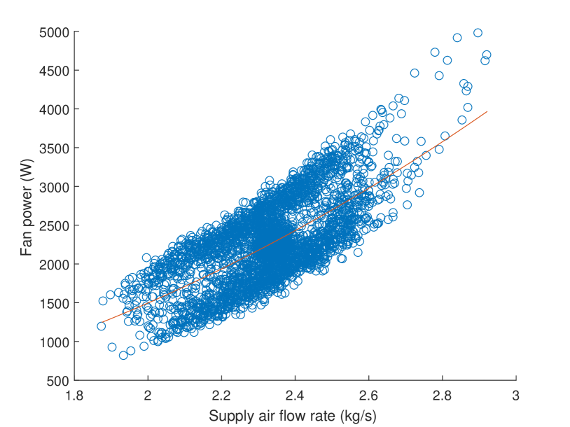
Figure 5: Fan power vs. airflow rate; measurements from AHU-2 of Pugh Hall at UF (circles), and predictions from the best fit model (9) to the measurements (curve).

The building in this paper is based on a large auditorium ($\sim 6$ m high, floor area of $\sim 465$ m²) in Pugh Hall located in the University of Florida campus, which is served by a dedicated air handling unit. We choose $m_{a}^{(b)}=2.27$ kg/s since that is representative of the airflow rate to this zone. We choose the following parameters, guided by [16]: $C=3.4\times 10^{7}$ J/K and $R=1.3\times 10^{-3}$ K/W. We also choose $T_{oa}=80^{\circ}$F and $COP=3.5$, somewhat arbitrarily. The fan power coefficients were chosen to be $\alpha_{1f}=662$ W/(kg/s)² and $\alpha_{2f}=-576$ W/(kg/s), based on fitting a quadratic model to measured fan power from the zone in question; see Figure 5.

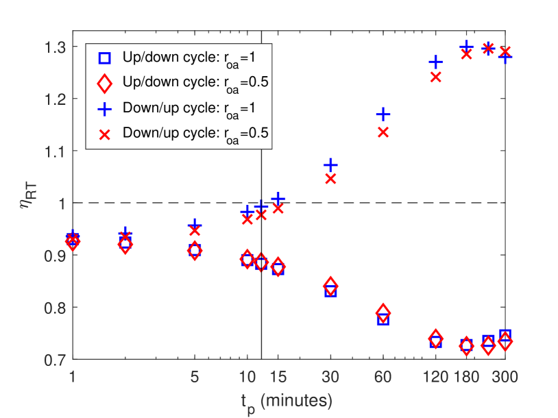
Figure 6: $\eta_{\textsc{rt}}$ vs. $t_{p}$, for $r_{oa}=1$ and $r_{oa}=0.5$; $\Delta P=0.2P^{(b)}_{\textsc{hvac}}$. The vertical line shown is $t_{p}^{*}$ ($\approx$12 minutes) computed from (24) for $r_{oa}=1$.

IV-B Multiple periods of square-wave power consumption

We now consider $n$ periods of the square-wave, $n>1$. At the end of $n$ periods, the temperature deviation may not be exactly 0 (i.e., $\tilde{T}(n2t_{p})\neq 0$), even though its initial value was $0$ (i.e., $\tilde{T}(0)=0$). Charging or discharging might be needed for an additional amount of time $t_{recov}$ to bring the temperature deviation back to $0$. Whether recovery to the initial SoC requires additional charging or additional discharging depends on whether $\tilde{T}(n2t_{p})$ is positive or negative. In either case, since $\tilde{T}(0)=\tilde{T}(n2t_{p}+t_{recov})=0$, according to Definition 1, the time interval $[0,\;n2t_{p}+t_{recov}]$ constitutes a complete charge-discharge interval of the virtual battery. The RTE computed over this interval using Definition 2 or equivalently (22) is called the RTE for n cycles or $\eta_{\textsc{rt}}(n)$.

Figure 7 shows an illustration of the two possible scenarios for the possible values of $\tilde{T}(n2t_{p})$. For the sake of concreteness, we have assumed the VES service starts with a down/up cycle in the figure.

Figure 7: Additional charging or discharging needed to bring $\tilde{T}$ to its initial value (=0) after $n$ periods of down/up cycle.

In the first possibility, denoted by the solid lines, $\tilde{T}(n2t_{p})\geq 0$, and therefore additional charging is performed for $t_{recov1}\geq 0$ amount of time in order to bring the temperature deviation to 0. If this possibility were to occur, within the complete charge-discharge interval of $[0,n2t_{p}+t_{recov1}]$, the charging time is $nt_{p}+t_{recov1}$, while the discharging time is $nt_{p}$. It now follows from (22) that for possibility 1

$$\eta_{\textsc{rt}}(n)=\frac{t_{d}}{t_{c}}=\frac{nt_{p}}{nt_{p}+t_{recov1}(n)}\leq 1.$$ (25)

In the second possibility, denoted by the dashed lines, $\tilde{T}(n2t_{p})\leq 0$ and therefore additional discharging is needed for $t_{recov2}\geq 0$ amount of time. For this possibility,

$$\eta_{\textsc{rt}}(n)=\frac{t_{d}}{t_{c}}=\frac{nt_{p}+t_{recov2}(n)}{nt_{p}}\geq 1.$$ (26)

If the VES service were to start with an up/down cycle, the same two possibilities exist in principle, so again the RTE can be smaller or larger than one depending on whether the temperature deviation at the end of the $n$ periods is positive or negative.

The proof of the main result of the paper, Theorem 1, needs a key intermediate result which is presented in the next lemma.

Lemma 2.

For $r_{oa}=1$ and $\tilde{T}(0)=0$, the magnitude of the temperature deviation $|\tilde{T}(t)|$ is bounded by $max\Big{\{}\lvert\tilde{T}_{c}^{ss}\rvert,|\tilde{T}_{d}^{ss}|\Big{\}},\,\forall t$ ($\tilde{T}_{c}^{ss}$ and $\tilde{T}_{d}^{ss}$ are defined in Proposition 1(c)).

The proof of Lemma 2 is presented in the Appendix.

Theorem 1.

If $r_{oa}=1$, $\lim_{n\to\infty}\eta_{\textsc{rt}}(n)=1$.

Proof of Theorem 1.

Consider the first possibility: $\tilde{T}(n2t_{p})\geq 0$ so that additional charging is needed for some time, and call that time $t_{recov}(n)\geq 0$. From (25), we have

$$\lim_{n\to\infty}\eta_{\textsc{rt}}(n)=\lim_{n\to\infty}\frac{nt_{p}}{nt_{p}+t_{recov}(n)}=\lim_{n\to\infty}\frac{t_{p}}{t_{p}+\frac{1}{n}t_{recov}(n)}.$$

Since the building is undergoing charging for $t>n2t_{p}$, it follows from Proposition 1(c) that the temperature deviation monotonically decays toward the value $\tilde{T}_{c}^{ss}$ from the “initial value” $\tilde{T}(n2t_{p})$. Since $\tilde{T}(n2t_{p})$ is bounded by a constant that is independent of $n$, which follows from Lemma 2, the time it takes for $\tilde{T}(t)$ to reach 0 from its “initial value” $\tilde{T}(n2t_{p})$ is upper bounded by a constant independent of $n$, which we denote by $\overline{t}_{recov}$. Thus, $t_{recov}(n)\leq\bar{t}_{recov}$, and $\bar{t}_{recov}$ is a constant independent of $n$. Therefore, $\lim_{n\to\infty}\frac{1}{n}t_{recov}(n)=0$, and therefore, $\lim_{n\to\infty}\eta_{\textsc{rt}}(n)=1$. A similar analysis holds for the  second possibility: $\tilde{T}(n2t_{p})\leq 0$. In this case additional discharging is needed for $t>n2t_{p}$. Again, the time it takes for the temperature deviation to get back to $0$ is upper bounded by a constant independent of $n$ since the “initial condition” $\tilde{T}(n2t_{p})$ is upper bounded (in magnitude) by a constant independent of $n$. Thus, again $\frac{1}{n}t_{recov}(n)\to 0$ as $n\to\infty$, and therefore $\lim_{n\to\infty}\eta_{\textsc{rt}}(n)$ = $\lim_{n\to\infty}\frac{nt_{p}+t_{recov}(n)}{nt_{p}}=1$. ∎

Comment 2.

1. Theorem 1 indicates that it is better for an HVAC-based virtual battery to provide VES services for an extended period of time, so that $n$ is large and hence RTE is close to 1. If VES service is stopped after a small number of cycles, RTE can be significantly lower than 1. This will entail a loss of efficiency and thus an increase in the energy cost for the building owner/operator.

2. Theorem 1 holds as long as the temperature deviation $\tilde{T}(t)$ is bounded by a constant independent of $t$, since that alone is sufficient to guarantee that $\frac{1}{n}t_{recov}(n)\to 0$ as $n\to\infty$. Therefore, the Theorem is robust to the kinds of model (and parameter values in the model) used in the analysis; the asymptotic RTE is 1 as long as the temperature deviation is bounded by a constant.

V Numerical verification

In order to show that the main result—Theorem 1—is robust to modeling assumptions made during analysis, we test the prediction using a more sophisticated model in simulations that includes humidity. The temperature dynamics are modeled as follows:

$$C_{z}\dot{T}(t) =\frac{1}{R_{w}}(T_{w}(t)-T(t))+q_{x}(t)+q_{\textsc{hvac}}(t)$$

$$C_{w}\dot{T}_{w}(t) =\frac{1}{R_{z}}(T_{oa}(t)-T_{w}(t))+\frac{1}{R_{w}}(T(t)-T_{w}(t))$$

where $T_{w}$ is the wall temperature, $C_{z}$ and $C_{w}$ are the thermal capacitance of the zone and the wall respectively, $R_{z}$ is the resistance to heat exchange between the outdoors and wall, and $R_{w}$ is the resistance to heat exchange between the wall and indoors. $q_{\textsc{hvac}}$ is the heat influx due to the HVAC system which is given by (8). The dynamics of zone humidity ratio $W$ is modeled as [17]:

$$\dot{W}(t)=\frac{R_{g}T(t)}{VP^{da}}\Bigg{[}\omega_{x}(t)+m_{a}(t)\frac{W_{sa}(t)-W(t)}{1+W_{sa}(t)}\Bigg{]}$$

where $V$ is the volume of dry air (which is same as the zone volume), $R_{g}$ is the specific gas constant of dry air, $P^{da}$ is the partial pressure of dry air, $W_{sa}$ is the supply air humidity ratio, and $\omega_{x}$ is the rate of internal water vapor generation. Models (9) and (10) are used to compute the fan and the chiller power respectively. Chiller $COP$ is modeled as a linear function of $T_{oa}$: $COP(t)=5.5-0.025T_{oa}(t)$, with $COP$ saturating at 4 for $T_{oa}\leq 60\degree F$ and 3 for $T_{oa}\geq 100\degree F$. This model is an approximation of the single-speed electric DX (direct expansion) air cooling coil model from [18].

The baseline power consumption is computed by performing a simulation with the climate control system. Then we perform the VES simulation with the square-wave power deviation reference added to the baseline power computed, which is provided as a power reference to the VES controller, as described in Section  III. At the end of the ancillary service event the VES controller is turned off and the zone climate controller is turned on to bring the zone temperature to its set point. Figure 8(a) shows numerically computed values of $\eta_{\textsc{rt}}(n)$ as a function of $n$. The RTE was computed using (6). The result presented in the figure is consistent with the prediction of Theorem 1 that the RTE tends to $1$ as $n\to\infty$.

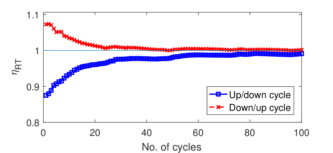
(a) $\eta_{\textsc{rt}}(n)$ vs. $n$, when the virtual battery tracks a square wave power reference ($\Delta P=4500$W, time period $=1$ hour).

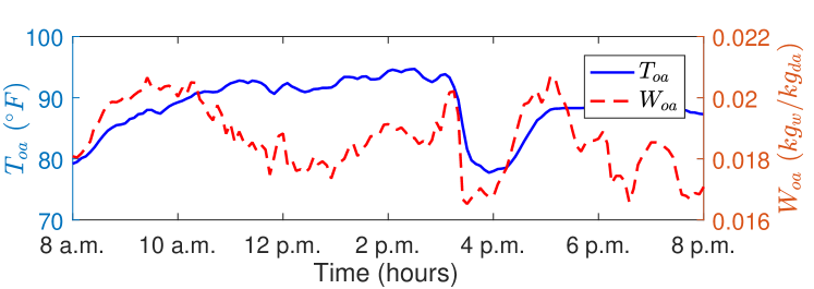
(b) Outside air temperature and humidity ratio used in simulations.

Figure 8: Robustness to modeling assumptions.

VI Conclusion

The main result of the paper is that the asymptotic RTE is unity. It is therefore better for an HVAC-based VES system to be used continuously for a long time than occasionally. The latter can cause low round trip efficiency, while the former has an efficiency close to $1$.

There are several additional avenues for further exploration. The discrepancy between our predictions and results in [5] for the “single demand-response event” calls for further studies; cf. Comment 1. Although the indoor temperature deviation is small (in the sub-1°F range) for the range of power deviations examined in our numerical simulations (5%-30%), the deviation is not zero mean. This can be interpreted as a slight warming—or cooling—of the building due to VES operation. Examination of the RTE, when the average temperature variation from the baseline is constrained to be 0, is ongoing and some preliminary progress in this direction has been reported in [19].

We start with a technical result first.

Proposition 2.

1. The parameter $a$ defined in (18) is positive for every positive $m_{a}$.

2. If $r_{oa}=1$, then $a^{2}>4d\Delta{P}$ for any feasible $\Delta P$.

3. If $r_{oa}=1$, then $\frac{a}{d}>m_{a}^{(b)}$.

4. If $r_{oa}=1$ and $\Delta P\leq P_{\textsc{hvac}}^{(b)}$, then $m_{a}^{(b)}\leq\dfrac{1}{2d}(a+\sqrt{a^{2}-4d\Delta P})$, with equality only if $\Delta P=P_{\textsc{hvac}}^{(b)}$.

Proof of Proposition 2.

1. It follows from  (18) that

   $$am_{a}^{(b)}=\alpha_{1f}(m_{a}^{(b)})^{2}+P_{\textsc{hvac}}^{(b)}.$$

   Since the right hand side is positive and $m_{a}^{(b)}>0$, we have that $a>0$.

2. For $r_{oa}=1$ it follows from (18) that:

   $$a=2\alpha_{1f}m_{a}^{(b)}+\alpha_{2f}+\frac{C_{pa}[T_{oa}-T_{sa}]}{COP}.$$

   The maximum value that $4d\Delta P$ can take is when $\Delta P=P_{\textsc{hvac}}^{(b)}$. Substituting for $\Delta P=P_{\textsc{hvac}}^{(b)}$ and from (19) we get:

   $$4\alpha_{1f}P_{\textsc{hvac}}^{(b)}=4\alpha_{1f}\Bigg{[}\alpha_{1f} (m_{a}^{(b)})^{2}+\alpha_{2f}m_{a}^{(b)}$$

   $$+\frac{m_{a}^{(b)}C_{pa}[T_{oa}-T_{sa}]}{COP}\Bigg{]}.$$

   So we need to prove that:

   $$\Bigg{[}2\alpha_{1f}m_{a}^{(b)}+\alpha_{2f}+\frac{C_{pa}[T_{oa}-T_{sa}]}{COP}\Bigg{]}^{2}>$$

   $$~{}~{}4\alpha_{1f}\Bigg{[}\alpha_{1f}(m_{a}^{(b)})^{2}+\alpha_{2f}m_{a}^{(b)}+\frac{m_{a}^{(b)}C_{pa}[T_{oa}-T_{sa}]}{COP}\Bigg{]}.$$

   This simplifies to

   $$\Bigg{[}\alpha_{2f}+\frac{C_{pa}[T_{oa}-T_{s}]}{COP}\Bigg{]}^{2}>0$$

   which is always true, and therefore $a^{2}>4d\Delta P$.

3. It follows from (18) and (19) that when $r_{oa}=1$

   $$\frac{a}{d}=\frac{2\alpha_{1f}m_{a}^{(b)}+\alpha_{2f}+\frac{C_{pa}[T_{oa}-T_{sa}]}{COP}}{\alpha_{1f}}.$$

   With further algebraic manipulation it reduces to $m_{a}^{(b)}+P_{\textsc{hvac}}^{(b)}/(\alpha_{1f}m_{a}^{(b)})$. Since $\alpha_{1f}$, $m_{a}^{(b)}$, and $P_{\textsc{hvac}}^{(b)}$ are positive, we have $a/d>m_{a}^{(b)}$.

4. Let us look at the following expression:

   $$\frac{a+\sqrt{a^{2}-4d\Delta P}}{2d}.$$ (27)

   Substituting for $\Delta P=P_{\textsc{hvac}}^{(b)}$ in the above expression and using the expressions for $a$ and $d$ from  (18) and (19) respectively, we get:

   $$\frac{2\alpha_{1f}m_{a}^{(b)}+\alpha_{2f}+\frac{C_{pa}[T_{oa}-T_{sa}]}{COP}+\mathinner{\!\left\lvert\alpha_{2f}+\frac{C_{pa}[T_{oa}-T_{sa}]}{COP}\right\rvert}}{2\alpha_{1f}}.$$ (28)

   If $\alpha_{2f}+\frac{C_{pa}[T_{oa}-T_{sa}]}{COP}>0$ then (28) becomes:

   $$m_{a}^{(b)}+\frac{\alpha_{2f}+\frac{C_{pa}[T_{oa}-T_{sa}]}{COP}}{\alpha_{1f}},$$

   which is greater than $m_{a}^{(b)}$ since $\alpha_{1f}>0$. If $\alpha_{2f}+\frac{C_{pa}[T_{oa}-T_{sa}]}{COP}<0$, then (28) becomes equal to $m_{a}^{(b)}$. In (27) for any $\Delta P<P_{\textsc{hvac}}^{(b)}$ the value of (27) increases and therefore is greater than $m_{a}^{(b)}$. This completes the proof.

∎

Proof of Proposition 1.

1. Since $r_{oa}=1$ from (19), $b=0$ and $c=0$. Therefore the solution for $\tilde{m}_{a}$ as a function of $\tilde{P}$ from (17) reduces to:

   $$\tilde{m}_{a}=\frac{-a\pm\sqrt{a^{2}+4d\tilde{P}}}{2d}.$$

   During charging $\tilde{P}=\Delta P$, so the the two roots in the equation above are $\frac{-a+\sqrt{a^{2}+4d\Delta P}}{2d}$ and $\frac{-a-\sqrt{a^{2}+4d\Delta P}}{2d}$. The second root is not possible, since it is negative with a minimum magnitude $\frac{+a+\sqrt{a^{2}}}{2d}=\frac{a}{d}$, which is larger than $m_{a}^{(b)}$ by Proposition 2(c), making the total airflow rate negative. Therefore during charging, the airflow rate is $\frac{-a+\sqrt{a^{2}+4d\Delta P}}{2d}$. This proves the first statement, regarding $\Delta m_{c}$. During discharging, $\tilde{P}=-\Delta P$, so the two possible roots are $\frac{-a+\sqrt{a^{2}-4d\Delta P}}{2d}$ and $\frac{-a-\sqrt{a^{2}-4d\Delta P}}{2d}$. The second root is not possible, since it is negative with a minimum magnitude larger than $m_{a}^{(b)}$ for $\Delta P<P_{\textsc{hvac}}^{(b)}$ from Proposition 2(d), which will make the total air flow rate negative. Therefore during charging, the airflow rate is $\frac{-a+\sqrt{a^{2}-4d\Delta P}}{2d}$. This proves the second statement, regarding $\Delta m_{d}$.

   To prove the inequality $\Delta m_{d}>\Delta m_{c}$, let $\nu\triangleq 4d\Delta P$ for simplifying the notation. The inequality $\Delta m_{d}>\Delta m_{c}$ is equivalent to:

   $$\frac{-a+\sqrt{a^{2}+\nu}}{2d}<\frac{a-\sqrt{a^{2}-\nu}}{2d}$$

   $$\Rightarrow-a+\sqrt{a^{2}+\nu}<a-\sqrt{a^{2}-\nu}\text{, as }d>0.$$

   Further algebraic manipulation gives,

   $$\sqrt{a^{2}+\nu}-\sqrt{a^{2}-\nu}>\frac{\nu}{a}.$$ (29)

   Since $a^{2}>\nu$ from Proposition 2(b), let us define $a^{2}=\nu+\epsilon$ where $\epsilon>0$. Therefore, (29) becomes:

   $$\sqrt{2\nu+\epsilon}-\sqrt{\epsilon}>\frac{\nu}{\sqrt{\nu+\epsilon}}$$

   $$\Rightarrow\sqrt{(2\nu+\epsilon)(\nu+\epsilon)}>\nu+\sqrt{\epsilon(\nu+\epsilon)}.$$

   Squaring on both sides yields:

   $$\Rightarrow\nu^{2}+2\nu\epsilon>2\nu\sqrt{\epsilon(\nu+\epsilon)},$$

   squaring again on both sides and simplifying, we get: $\nu^{4}>0$, which is true, and therefore $\Delta m_{c}<\Delta m_{d}$.

2. Note that the maximum value that $\Delta m_{d}$ can take is $m_{a}^{(b)}$; otherwise, the total airflow rate will be negative. For that value of $\Delta m_{d}$, $\gamma\Delta m_{d}=\frac{C_{pa}m_{a}^{(b)}}{C}$ (as $\gamma=C_{pa}/C$). Substituting for $\alpha$ from (21) and since $R,C>0$, we have $\frac{C_{pa}m_{a}^{(b)}}{C}+\frac{1}{RC}>\frac{C_{pa}m_{a}^{(b)}}{C}$ so that $\alpha>\gamma\Delta m_{d}$. For the second inequality, note that from Proposition1(a) $\Delta m_{c}<\Delta m_{d}$. Since $\gamma$ is positive, $\gamma\Delta m_{c}<\gamma\Delta m_{d}$. Therefore, $\alpha>\gamma\Delta m_{d}>\gamma\Delta m_{c}$.

3. We have already proved above that, $\tilde{m}_{a}(t)\equiv\Delta m_{c}$ when charging and $\tilde{m}_{a}(t)\equiv-\Delta m_{d}$ when discharging. It follows from (20) that the temperature dynamics reduce in the charging scenario to

   $$\dot{\tilde{T}}(t)=-(\alpha+\gamma\Delta m_{c})\tilde{T}-\beta\Delta m_{c},$$ (30)

   and in the discharging scenario to

   $$\dot{\tilde{T}}(t)=-(\alpha-\gamma\Delta m_{d})\tilde{T}+\beta\Delta m_{d}.$$ (31)

   Both of these are linear time invariant systems driven by constant inputs that are asymptotically stable; stability follows from $\alpha>\gamma\Delta m_{d}$, which was proved above and $\alpha$, $\gamma$, and $\Delta m_{c}$ being positive. It follows from elementary linear systems analysis [20] that $\tilde{T}(t)$ converges to a constant steady-state value irrespective of the initial condition, which is, in the charging scenario: $\tilde{T}_{c}^{ss}=\frac{\beta\Delta m_{c}}{-(\alpha+\gamma\Delta m_{c})}$, and in the discharging scenario: $\tilde{T}_{d}^{ss}=\frac{\beta\Delta m_{d}}{(\alpha-\gamma\Delta m_{d})}$. Since $\alpha$, $\beta$, $\gamma$, $\Delta m_{c}$ and $\Delta m_{d}$ are all positive, $\tilde{T}_{c}^{ss}<0$, and the fact that $\tilde{T}_{d}^{ss}>0$ follows from Proposition 1(b), proved above.  
   For the second part of the statement, we need to prove that

   $$\frac{\beta\Delta m_{c}}{(\alpha+\gamma\Delta m_{c})}<\frac{\beta\Delta m_{d}}{(\alpha-\gamma\Delta m_{d})}.$$ (32)

   It follows from Proposition 1(b) that $\alpha+\gamma\Delta m_{c}>\alpha-\gamma\Delta m_{c}>0$. Therefore, and since all relevant parameters are positive,

   $$\frac{\beta\Delta m_{c}}{\alpha+\gamma\Delta m_{c}} <\frac{\beta\Delta m_{c}}{\alpha-\gamma\Delta m_{c}}.$$ (33)

   Again from Proposition 1(b), we get

   $$\frac{\beta\Delta m_{c}}{\alpha+\gamma\Delta m_{c}} <\frac{\beta\Delta m_{c}}{\alpha-\gamma\Delta m_{c}}<\frac{\beta\Delta m_{d}}{\alpha-\gamma\Delta m_{d}},$$ (34)

   where the second inequality follows from $\Delta m_{c}<\Delta m_{d}$. Thus from (34) we get the desired inequality (32), which proves the second statement.

∎

Now we are ready to prove Lemma 1.

Proof of Lemma 1.

Since $r_{oa}=1$, recall that we established in the proof of Proposition 1(c) that $\tilde{T}(t)$ is governed by two asymptotically stable linear time invariant systems, with step inputs, (30) and (31), during the charging and discharging half-periods respectively. Consider first the up/down scenario, with initial condition $\tilde{T}(0)=0$. By solving the two differential equations (30)-(31), we obtain the temperature deviation at the end of one period of the square wave:

$$\tilde{T}(2t_{p}) =\frac{-\beta\Delta m_{c}e^{-(\alpha-\gamma\Delta m_{d})t_{p}}(1-e^{-(\alpha+\gamma\Delta m_{c})t_{p}})}{\alpha+\gamma\Delta m_{c}}$$

$$\quad+\frac{\beta\Delta m_{d}(1-e^{-(\alpha-\gamma\Delta m_{d})t_{p}})}{\alpha-\gamma\Delta m_{d}}.$$

By hypothesis, $(\alpha-\gamma\Delta m_{d})t_{p}<(\alpha+\gamma\Delta m_{c})t_{p}\ll 1$, so we can use a first order Taylor expansion to get the following approximation:

$$\tilde{T}(2t_{p})\approx t_{p}\beta\left(\Delta m_{d}-\Delta m_{c}e^{-(\alpha-\gamma\Delta m_{d})t_{p}}\right).$$ (35)

Since $\Delta m_{c}<\Delta m_{d}$ and $(\alpha-\gamma\Delta m_{d})>0$, we get $\tilde{T}(2t_{p})>0$. This is possibility 1 shown in Figure 3: $t_{d}=t_{p}$, while $t_{c}=t_{p}+t_{recov}$ for some $t_{recov}>0$. It follows from (22) that $\eta_{\textsc{rt}}<1$. Consider second the down/up scenario, with initial condition $\tilde{T}(0)=0$. The corresponding expression becomes:

$$\tilde{T}(2t_{p}) =\frac{\beta\Delta m_{d}e^{-(\alpha+\gamma\Delta m_{c})t_{p}}(1-e^{-(\alpha-\gamma\Delta m_{d})t_{p}})}{\alpha-\gamma\Delta m_{d}}$$

$$\quad-\frac{\beta\Delta m_{c}(1-e^{-(\alpha+\gamma\Delta m_{c})t_{p}})}{\alpha+\gamma\Delta m_{c}}.$$

A similar approximation gives:

$$\tilde{T}(2t_{p})\approx t_{p}\beta\left(e^{-(\alpha+\gamma\Delta m_{c})t_{p}}\Delta m_{d}-\Delta m_{c}\right).$$ (36)

As long as $t_{p}>t_{p}^{*}$, we have $e^{-(\alpha+\gamma\Delta m_{c})t_{p}}<\Delta m_{c}/\Delta m_{d}$, and thus $\tilde{T}(2t_{p})<0$. This is possibility 2 shown in Figure 4: $t_{c}=t_{p}$, while $t_{d}=t_{p}+t_{recov}$ for some $t_{recov}>0$. It now follows from (22) that $\eta_{\textsc{rt}}>1$. However, if $t_{p}<t_{p}^{*}$, then $e^{-(\alpha+\gamma\Delta m_{c})t_{p}}>\Delta m_{c}/\Delta m_{d}$, and we have $\tilde{T}(2t_{p})>0$. This is possibility 1 shown in Figure 4: $t_{d}=t_{p}$, while $t_{c}=t_{p}+t_{recov}$ for some $t_{recov}>0$, and it follows from (22) that $\eta_{\textsc{rt}}<1$. ∎

Proof of Lemma 2.

Recall that we established in the proof of Proposition 1(c) that $\tilde{T}(t)$ is governed by two asymptotically stable, linear, time invariant systems, with step inputs, (30) and (31), during the charging and discharging half-periods respectively. It follows from elementary linear systems theory that the step response of a stable first-order LTI system monotonically increases (or decreases, depending on the initial condition) towards the steady-state value. Therefore, in the time interval $[0,t_{p}]$, the maximum value of $|\tilde{T}(t)|$ will be (depending on whether the system is charging or discharging)

$$\lvert\tilde{T}(t)\rvert \leq max\Big{\{}\lvert\tilde{T}(0)\rvert,|\tilde{T}_{c}^{ss}|,|\tilde{T}_{d}^{ss}|\Big{\}},\quad\forall t\in[0,t_{p}].$$ (37)

The value of $\tilde{T}(t_{p})$ will serve as the initial condition to the LTI dynamics that govern $\tilde{T}(t)$ during the interval $[t_{p},2t_{p}]$, which is either (30) or (31). Using the same argument, we see that the maximum value of $|\tilde{T}(t)|$ in this time interval will satisfy

$$\lvert\tilde{T}(t)\rvert \leq max\Big{\{}\lvert\tilde{T}(t_{p})\rvert,\lvert\tilde{T}_{c}^{ss}\rvert,|\tilde{T}_{d}^{ss}|\Big{\}},\quad\forall t\in[t_{p},2t_{p}],$$

$$\leq max\Big{\{}\lvert\tilde{T}(0)\rvert,\lvert\tilde{T}_{c}^{ss}\rvert,|\tilde{T}_{d}^{ss}|\Big{\}},\quad\forall t\in[0,t_{p}],$$

where the second inequality follows from combining the first inequality with (37). Since $\tilde{T}(2t_{p})$ serves as the initial condition for the second period $[2t_{p},4t_{p}]$ and so on, we can repeat this argument ad infinitum, and arrive at the conclusion that $|\tilde{T}(t)|$, for any $t\geq 0$, is bounded by the constants $\lvert\tilde{T}(0)\rvert,\lvert\tilde{T}_{c}^{ss}\rvert,\text{ and }|\tilde{T}_{d}^{ss}|$. Since $\tilde{T}(0)=0$, $max\Big{\{}\lvert\tilde{T}(0)\rvert,|\tilde{T}_{c}^{ss}|,|\tilde{T}_{d}^{ss}|\Big{\}}=max\Big{\{}|\tilde{T}_{c}^{ss}|,|\tilde{T}_{d}^{ss}|\Big{\}}$. Therefore, $|\tilde{T}(t)|$, for any $t\geq 0$, is bounded by the constants $\lvert\tilde{T}_{c}^{ss}\rvert,|\tilde{T}_{d}^{ss}|$, which proves the statement. ∎

References

- [1] Y. Makarov, J. Ma, S. Lu, and T. Nguyen, “Assessing the value of regulation resources based on their time response characteristics,” Pacific Northwest National Laboratory, 2008.
- [2] Y. Lin, P. Barooah, S. Meyn, and T. Middelkoop, “Experimental evaluation of frequency regulation from commercial building HVAC systems,” IEEE Transactions on Smart Grid, vol. 6, pp. 776 – 783, 2015.
- [3] M. Cheng, S. S. Sami, and J. Wu, “Benefits of using virtual energy storage system for power system frequency response,” Applied Energy, vol. 194, no. Supplement C, pp. 376 – 385, 2017.
- [4] X. Luo, J. Wang, M. Dooner, and J. Clarke, “Overview of current development in electrical energy storage technologies and the application potential in power system operation,” Applied Energy, vol. 137, pp. 511 – 536, 2015.
- [5] I. Beil, I. Hiskens, and S. Backhaus, “Round-trip efficiency of fast demand response in a large commercial air conditioner,” Energy and Buildings, vol. 97, no. 0, pp. 47 – 55, 2015.
- [6] Y. Lin, J. L. Mathieu, J. X. Johnson, I. A. Hiskens, and S. Backhaus, “Explaining inefficiencies in commercial buildings providing power system ancillary services,” Energy and Buildings, vol. 152, pp. 216 – 226, 2017.
- [7] PJM, “PJM manual 12: Balancing operations, rev. 27,” December 2012.
- [8] Y. Lin, P. Barooah, S. Meyn, and T. Middelkoop, “Demand side frequency regulation from commercial building HVAC systems: An experimental study,” in American Control Conference, 2015, pp. 3019 – 3024.
- [9] E. Vrettos, E. C. Kara, J. MacDonald, G. Andersson, and D. S. Callaway, “Experimental demonstration of frequency regulation by commercial buildings; part ii: Results and performance evaluation,” IEEE Transactions on Smart Grid, vol. PP, no. 99, pp. 1–1, 2017.
- [10] K. S. Ng, C.-S. Moo, Y.-P. Chen, and Y.-C. Hsieh, “Enhanced coulomb counting method for estimating state-of-charge and state-of-health of lithium-ion batteries,” Applied Energy, vol. 86, no. 9, pp. 1506 – 1511, 2009.
- [11] V. Sprenkle, D. Choi, A. Crawford, and V. Viswanathan, “(invited) Life-cycle comparison of EV Li-ion battery chemistries under grid duty cycles,” Meeting Abstracts, vol. MA2017-02, no. 4, p. 218, 2017.
- [12] R. Kramer, J. van Schijndel, and H. Schellen, “Simplified thermal and hygric building models: A literature review,” Frontiers of Architectural Research, vol. 1, no. 4, pp. 318 – 325, 2012.
- [13] S. F. Fux, A. Ashouri, M. J. Benz, and L. Guzzella, “EKF based self-adaptive thermal model for a passive house,” Energy and Buildings, vol. 68, Part C, pp. 811 – 817, 2014.
- [14] C.-A. Roulet, F. Heidt, F. Foradini, and M.-C. Pibiri, “Real heat recovery with air handling units,” Energy and Buildings, vol. 33, no. 5, pp. 495 – 502, 2001.
- [15] S. Mallat, A wavelet tour of signal processing: the sparse way. Academic press, 2008.
- [16] Y. Lin, “Control of commercial building HVAC systems for power grid ancillary services,” Ph.D. dissertation, University of Florida, August 2014.
- [17] S. Goyal and P. Barooah, “A method for model-reduction of non-linear thermal dynamics of multi-zone buildings,” Energy and Buildings, vol. 47, pp. 332–340, April 2012.
- [18] U.S. DOE, “EnergyPlus engineering reference: The reference to EnergyPlus calculations,” Lawrence Berkeley National Laboratory, 2018.
- [19] N. Raman and P. Barooah, “Analysis of round-trip efficiency of an HVAC-based virtual battery,” in 5th International Conference on High Performance Buildings, July 2018, pp. 1–10.
- [20] H. Kwakernaak and R. Sivan, Linear Optimal Control Systems. Wiley-Interscience, 1972.