Stochastic Games for Fuel Followers Problem: $N$ versus MFG

Abstract

In this paper we formulate and analyze an $N$-player stochastic game of the classical fuel follower problem and its Mean Field Game (MFG) counterpart. For the $N$-player game, we obtain the Nash Equilibrium (NE) explicitly by deriving and analyzing a system of Hamilton–Jacobi–Bellman (HJB) equations, and by establishing the existence of a unique strong solution to the associated Skorokhod problem on an unbounded polyhedron with an oblique reflection. For the MFG, we derive a bang-bang type NE under some mild technical conditions and by the viscosity solution approach. We also show that this solution is an $\epsilon$-NE to the $N$-player game, with $\epsilon=O(\frac{1}{\sqrt{N}})$. The $N$-player game and the MFG differ in that the NE for the former is state dependent while the NE for the latter is threshold-type bang-bang policy where the threshold is state independent . Our analysis shows that the NE for a stationary MFG may not be the NE for the corresponding MFG.

1 Introduction

The classic fuel follower problem concerns controlling a single moving object on a real line whose movement is modeled by a standard Brownian motion. The controller controls the position of her object in a possibly non-continuous way, i.e., with singular controls. Her objective is to minimize over an infinite-time horizon, the total amount of control and the total $L^{2}$ distance of the object to the origin, with a discount factor. The optimal control derived by Beneš, Shepp, and Witsenhausen [4] is shown to be of a “bang-bang” type. That is, there exists a threshold $c$ such that when the object is within $[-c,c]$, it will be idling; and when it is outside $[-c,c]$, the controller will apply the minimal push needed to bring it back within $[-c,c]$. The controlled dynamics is thus a reflected Brownian motion, with local times at $c$ and $-c$ as a result of the minimal push. This problem has a number of generalizations; see, for example, Karatzas [29], Karatzas and Shreve [31], and Shreve and Soner [39]. In particular, Karatzas [29] derives a similar bang-bang type optimal control when the $L^{2}$ distance is relaxed to a class of convex and symmetric functions; see Figure 1. Due to its simplicity, the fuel follower problem has many applications and has inspired a number of research topics, including reflected stochastic differential equations and semimartingales, Skorokhod problems, and regularities of fully nonlinear PDEs with gradient constraints. See, for instance, Harrison and Williams [23], Soner and Shreve [41], Varadhan and Williams [42], Williams [43], Dai and Williams [14], Kruk [33], Atar and Budhiraja [1], Budhiraja and Ross [7], Evans [18], and Hynd [28].

Our work.

In this paper we formulate and analyze an $N$-player stochastic game of the fuel follower problem and its Mean Field Game (MFG) counterpart. In the $N$-player game, there are $N$ controllers and $N$ objects with each controller controlling one object. Each controller minimizes her total amount of control and the total distance of her object to the center of the $N$ objects. The interaction among the $N$ controllers in the game is to ensure that their own objects closely follow each other’s movement. We derive the Nash Equilibrium (NE) explicitly (Theorem 5). This result is established in two main steps. The first step is to derive and analyze a system of Hamilton–Jacobi–Bellman (HJB) equations for the value functions and to establish a verification theorem (Theorem 3) for the game. After finding the solution to the HJB system, the second step is to construct a feedback control via proving the existence of a (unique strong) solution to an associated Skorokhod problem on an unbounded polyhedron with an oblique reflection (Theorem 4). For the special case of $N=2$, we exploit the symmetric structure to obtain multiple NEs; see Figure 4.

We then consider the corresponding MFG with $N\to\infty$, where each controller minimizes her total amount of control and the total distance of her object to the mean position of all objects. Our approach to analyze this MFG is to study directly the two coupled PDEs, the backward parabolic type HJB equation and the forward Kolmogorov equation. By further exploiting the problem structure, we derive an NE which is of a bang-bang type (Theorem 7). The threshold of this bang-bang type NE is state-independent as in the classical fuel follower problem. We finally discuss the relation between the $N$-player game and the MFG, and show that this NE to the MFG game is an $\epsilon$-NE to the $N$-player game (Theorem 14).

Our contribution.

In general, there are essential technical difficulties in analyzing $N$-player stochastic games. The underlying HJB system is high dimensional, the existence of its solution is usually hard to analyze, and deriving explicit solutions is even more challenging. Therefore it is in general infeasible to characterize the equilibrium. In the case of the singular control, the HJB equation is even more complex, with additional gradient constraints coming from possible jumps in the control. For MFGs with singular controls, the Hamiltonian for the underlying stochastic control problem diverges and the classical stochastic maximal principle fails. Moreover, due to the possible non-stationarity of the mean information process, the associated HJB equation is parabolic despite the infinite-time horizon setting, making it even more difficult to analyze the regularity of the value functions or to derive explicit solutions.

To the best of our knowledge, our work is the first to provide a complete characterization of the NEs for both the $N$-player stochastic game and the MFG in a singular control setting. Our explicit solutions are derived for a class of convex and symmetric functions, without the usual linear-quadratic structure for MFGs with regular controls in Bardi [2], Bardi and Priuli [3], Bensoussan, Sung, Yam, and Yung [6].

Moreover, explicit solutions derived in this paper make it possible to directly compare the structural differences between the MFG and the $N$-player game. It provides useful insights not only for analyzing general $N$-player games but also for proper formulations of MFGs. Indeed, MFGs may be very different in nature from $N$-player games: in the fuel follower problem, the MFG degenerates to a single-player game in the sense that its NE is threshold-type bang-bang policy where the threshold is state independent (Proposition 11 and Proposition 12), while the NEs for the $N$-player game are state dependent (Theorem 5). The collapse of the MFG to the single player problem (Proposition 11) is a side effect by the aggregation in the MFG formulation: players become more anticipative when they are assumed to be identical. Our analysis also shows that the NE for a stationary MFG may not be the NE for the corresponding MFG (Remark 10.1).

There are also some noteworthy economic insights from our analysis. For instance, in the $N$-player game, we show that when the number of players increases, it is more costly for each player to keep track of other players before making decisions, as players will intervene more frequently due to the increasing complexity of the game. Moreover, the bigger the discount factor $\alpha$, the less frequent players will intervene. (See Remarks 15.1 and 12.1).

Related work on stochastic games.

There are a number of papers on non-zero-sum two-player games with singular controls. By treating one as a controller and the other as a stopper, where the controller minimizes the finite variation process and the stopper decides the optimal time to terminate the game, Karatzas and Li [30] prove the existence of an NE for the game via a BSDE approach. Hernandez-Hernandez, Simon, and Zervos [24] provide an in-depth analysis of the smoothness of the value function and show that the optimal strategy may not be unique when the controller enjoys a first-move advantage. Kwon and Zhang [34] investigate a game of irreversible investment with singular controls and strategic exit. They characterize a class of market perfect equilibria and identify a set of conditions under which the outcome of the game may be unique despite the multiplicity of the equilibria. De Angelis and Ferrari [15] establish the connection between singular controls and optimal stopping times for a non-zero-sum two-player game. Bensoussan and Frehse [5] consider an $N$-player game with regular controls and obtain the NE via the maximum principle approach. The closest to our problem setting are those of Mannucci [37] and Hamadene and Mu [22]. They consider the fuel follower problem in a finite-time horizon with a bounded velocity, and establish the existence of an NE of a two-player game. The former analyzes a strongly coupled parabolic system and the latter uses the BSDE technique.

Related work on MFGs.

The theory of MFGs has enjoyed tremendous growth since the pioneering works of Huang, Malhamé, and Caines [27] and Lasry and Lions [36]. The MFG provides a tractable approach to the otherwise challenging $N$-player stochastic games. However, except for the general result that the NE of an MFG is an $\epsilon$-Nash equilibrium to the $N$-player game (see, for instance [27] and Cardaliaguet, Delarue, Lasry, and Lions [10] for regular controls and Guo and Joon [20] for singular controls), there are very limited results on comparing the NE of $N$-player games and MFGs. The exceptions are Carmona, Fouque, and Sun [12] for systemic risks, Nutz and Zhang [38] for competition, Lacker and Zariphopoulou [35] for portfolio management, and [2]. All these results, however, are with regular controls. For MFGs with singular controls, notions of relaxed stochastic maximal principle or relaxed admissible controls have been introduced to establish the existence of optimal controls; see, for instance, Fu and Horst [19], Hu, Øksendal, and Sulem [25], and Zhang [44].

2 $N$-Player Fuel Follower Game

2.1 Preliminary: Single Player

The classic fuel follower problem is as follows. Consider a probability space $(\Omega,\mathcal{F},$ $\{\mathcal{F}_{t}\}_{t\geq 0},\mathbb{P})$ with a standard Brownian motion $\{B_{t}\}_{t\geq 0}$. The position of the object $X_{t}$ is assumed to be

$$X_{t}=x+B_{t}+\xi_{t}^{+}-\xi_{t}^{-},\quad X_{0-}=x,$$ (2.1)

where the pair of control $(\xi^{+},\xi^{-})$ is a non-decreasing, càdlàg process. The goal of the controller is to solve for the value function $v(x)$ of the following optimization problem,

$$v(x)=\inf_{(\xi^{+},\xi^{-})\in\mathcal{U}}\mathbb{E}\int_{0}^{\infty}e^{-\alpha t}\left[h(X_{t})dt+d\check{\xi}_{t}\right],$$ (2.2)

where the admissible control set $\cal U$ is

$$\mathcal{U} :=\left\{(\xi_{t}^{+},\xi_{t}^{-})\>\lvert\>\xi_{t}^{+}\mbox{ and }\xi_{t}^{-}\mbox{ are }\textrm{$\mathcal{F}^{X_{t-}}$-progressively measurable, c\`{a}dl\`{a}g, non-decreasing},\right.$$

$$\left.\hskip 63.0pt\textrm{ with }\mathbb{E}\left[\int_{0}^{\infty}e^{-\alpha t}d\xi_{t}^{+}\right]<\infty,\mathbb{E}\left[\int_{0}^{\infty}e^{-\alpha t}d\xi_{t}^{-}\right]<\infty,\textrm{and }\xi_{0-}^{+}=\xi_{0-}^{-}=0\right\}.$$

Here $\alpha>0$ is a discount factor, $\{\mathcal{F}^{X_{t}}\}_{t\geq 0}$ is the natural filtration of $\{X_{t}\}_{t\geq 0}$, and $\check{\xi_{t}}=\xi_{t}^{+}+\xi_{t}^{-}$ is the total accumulative amount of controls up to time t, called “fuel usage”, hence the term fuel follower problem. In addition, under the assumption

• The function $h:\mathbb{R}\rightarrow\mathbb{R}$ is assumed to be convex, symmetric, twice differentiable, with $h(0)\geq 0$, $h^{\prime\prime}(x)$ decreasing on $\mathbb{R}^{+}$, and $0<k<h^{\prime\prime}(x)\leq K$ for some constants $K>k>0$,

Problem (2.2) is solved (see [4] and [29]) by analyzing the associated HJB equation

$$\min\left\{\frac{1}{2}v_{xx}(x)+h(x)-\alpha v(x),1-v_{x}(x),1+v_{x}(x)\right\}=0,$$ (2.3)

where $v_{x}$ and $v_{xx}$ are the first and second order derivatives of $v$ with respect to $x$, respectively. The optimal control $\{\xi_{t}^{*+},\xi_{t}^{*-}\}_{t\geq 0}$ is shown to be of a bang-bang type given by

$$\xi_{t}^{*+} = \max\left\{0,\max_{0\leq u\leq t}\left\{-x-{B}_{u}+\xi_{u}^{*-}-c\right\}\right\},$$

$$\xi_{t}^{*-} = \max\left\{0,\max_{0\leq u\leq t}\left\{x+{B}_{u}+\xi_{u}^{*+}-c\right\}\right\},$$

where the threshold $c>0$ is the unique positive solution to

$$\frac{1}{\sqrt{2\alpha}}\tanh\left(c\sqrt{2\alpha}\right)=\frac{p_{1}^{{}^{\prime}}(c)-1}{p_{1}^{{}^{\prime\prime}}(c)},$$ (2.4)

with

$$p_{1}(x) = \mathbb{E}\left[\int_{0}^{\infty}e^{-\alpha t}h(x+B_{t})dt\right]$$

$$= \frac{1}{\sqrt{2\alpha}}\left(e^{-x\sqrt{2\alpha}}\int_{-\infty}^{x}h(z)e^{z\sqrt{2\alpha}}dz+e^{x\sqrt{2\alpha}}\int_{x}^{\infty}h(z)e^{-z\sqrt{2\alpha}}dz\right).$$

The corresponding value function $v(x)\in\mathcal{C}^{2}(\mathbb{R})$ is given by

$$v(x)=\left\{\begin{array}[]{ll}-\frac{p_{1}^{\prime\prime}(c)\cosh\left(x\sqrt{2\alpha}\right)}{2\alpha\cosh\left(c\sqrt{2\alpha}\right)}+p_{1}(x),\qquad\ \ 0\leq&x\leq c,\\ v(c)+(x-c),&x\geq c,\\ v(-x),&x<0.\end{array}\right.$$ (2.8)

In other words, it is optimal for the controller to apply a “minimal” push to keep the object within $[-c,c]$. Mathematically, the controlled process is a Brownian motion reflected at the boundaries $c$ and $-c$. The minimal push corresponds to the local time of the Brownian motion at $c$ and $-c$. See Figure 1.

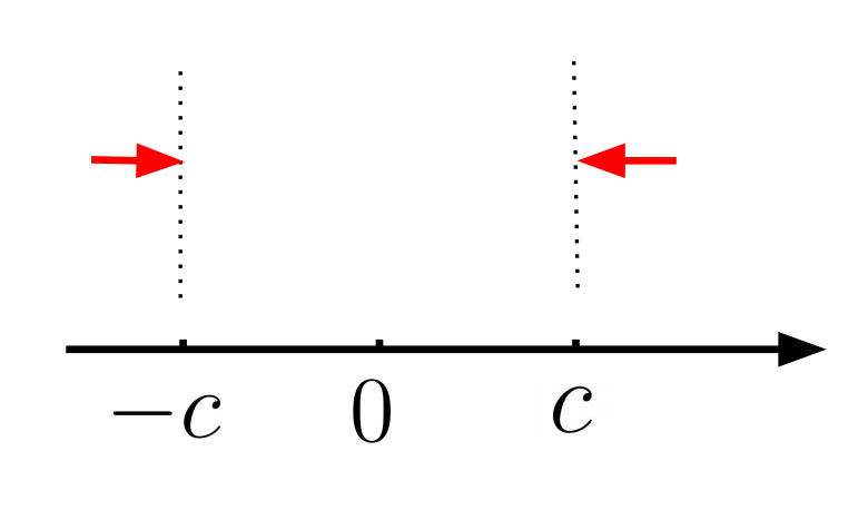
Figure 1: Optimal control of the single player problem

2.2 $N$-Player Fuel Follower Game

Now suppose there are $N$ controllers, with each controller controlling one object. For simplicity, let us call such a pair of controller and object a “player”. The game is for each player to stay as close as possible to other players.

This $N$-player game can be formulated as follows. Let $\left(X_{t}^{1},\ldots,X_{t}^{N}\right)\in\mathbb{R}^{N}$ be the positions of players such that for $i=1,\ldots,N$,

$$X_{t}^{i}=x^{i}+B_{t}^{i}+\xi_{t}^{i,+}-\xi_{t}^{i,-},$$ (2.9)

with $(X_{0-}^{1},\cdots,X_{0-}^{N})=(x^{1},\cdots,x^{N})=:\boldsymbol{x}$, where $(B_{t}^{1},\ldots,B_{t}^{N})$ is an $N$-dimensional standard Brownian motion on $\mathbb{R}^{N}$. Let $m_{t}^{(N)}=\frac{\sum_{i=1}^{N}X_{t}^{i}}{N}$ be the center of these $N$ players at time $t$, with $m_{0-}^{(N)}=\frac{\sum_{i=1}^{N}x^{i}}{N}$. Let $h(X_{t}^{i}-m_{t}^{(N)})$ be the distance between player $i$ and the center $m_{t}^{(N)}$ at time $t$. The goal of each player $i$ is to minimize, over all admissible controls $\left(\xi^{1},\ldots,\xi^{N}\right)\in\mathcal{S}_{N}$, the following payoff function

$$J^{i}(x^{1},\ldots,x^{N};\xi^{1},\ldots,\xi^{N})=\mathbb{E}\int_{0}^{\infty}e^{-\alpha_{i}t}\left[h\left(X^{i}_{t}-\rho m_{t}^{(N)}\right)dt+d\check{\xi}_{t}^{i}\right],$$

where $\check{\xi}^{i}={\xi}^{i,+}+{\xi}^{i,-}$. Here the admissible control set $\mathcal{S}_{N}$ is defined as

$$\begin{aligned} \mathcal{S}_{N}:=&\left\{(\xi^{1},\ldots,\xi^{N})\ \left|\ \xi^{j}=(\xi^{j,+},\xi^{j,-})\in\mathcal{U}^{j}_{N},\mathbb{P}\left(d\xi_{t}^{j}(\boldsymbol{x})d\xi_{t}^{i}(\boldsymbol{x})>0\right)=0,\right.\right.\\ &\hskip 70.0pt\left.\mbox{ for any }t>0,\boldsymbol{x}\in\mathbb{R}^{N},i,j\in\{1,\ldots,N\}\mbox{ and }i\neq j\right\},\end{aligned}$$ (2.9)

with

$$\begin{aligned} \mathcal{U}^{j}_{N}=&\left\{(\xi_{t}^{j,+},\xi_{t}^{j,-})\ \left|\ \xi_{t}^{j,+}\mbox{ and }\xi_{t}^{j,-}\mbox{ are }\mathcal{F}^{(X^{1}_{t-},\ldots,X^{N}_{t-})}\mbox{-progressively measurable, c\`{a}dl\`{a}g, non-decreasing,}\right.\right.\\ &\hskip 50.0pt\left.{}\mbox{ with }\mathbb{E}\left[\int_{0}^{\infty}e^{-\alpha_{j}t}d\xi_{t}^{j,+}\right]<\infty,\enspace\mathbb{E}\left[\int_{0}^{\infty}e^{-\alpha_{j}t}d\xi_{t}^{j,-}\right]<\infty,\enspace\xi_{0-}^{j,+}=0,\enspace\xi_{0-}^{j,-}=0\right\},\end{aligned}$$

where $\alpha_{j}>0$ is the discount factor for player $j$ and $\{\mathcal{F}^{(X_{t}^{1},\ldots,X_{t}^{N})}\}_{t\geq 0}$ is the natural filtration of $\{(X_{t}^{1},\ldots,X_{t}^{N})\}_{t\geq 0}$. The condition in Eqn. (2.9)

$$\mathbb{P}\left(d\xi_{t}^{i}(\boldsymbol{x})d\xi_{t}^{j}(\boldsymbol{x})>0\right)=0,\ \ \ \ \mbox{ for any }\boldsymbol{x}\in\mathbb{R}^{N},t\geq 0,i\neq j$$ (2.10)

is to facilitate designing feasible control policies when controls involve jumps.

Remark 0.1.

Mathematically, one may replace the running cost function $h(X_{t}^{i}-m_{t}^{N})$ by $h(X_{t}^{i}-\rho m_{t}^{N}+\eta)$, with $\rho\geq 0$ indicating the strength of interactions among players as in [26] and [27]. We choose to fix $\rho=1$ and $\eta=0$ for clearer model interpretations for the fuel follower problem. Indeed, adding a scaling factor $\rho$ and a constant $\eta$ will not change the derivation of solutions except for minor notational changes. In fact, as will be shown in Section 2.6 and Appendix A, the construction of NEs will be simpler when $\rho\neq 1$.

Throughout the paper, unless otherwise specified, we will for simplicity and without loss of generality $\alpha_{1}=\cdots=\alpha_{N}=\alpha$. (See Section 5 for further sensitivity analysis with respect to $\alpha$.)

2.3 Solution to the $N$-Player Game

There are various criteria to measure the performance of strategies in stochastic games. For instance, Pareto Optimality (PO) and Nash Equilibrium (NE) provide two distinct views, with NE focusing on stability and PO on efficiency. An NE framework can be further defined depending on the admissible strategies, resulting in open-loop NEs, closed-loop NEs, and the Markovian NEs. See Carmona [11] for more discussions on these concepts.

In this paper, we will focus on the Markovian NE, also known as the closed-loop NE with a feedback form, specified below.

Definition 1.

A tuple of admissible controls $\boldsymbol{\xi}^{*}=({\xi}^{1*},\ldots,{\xi}^{N*})\in\mathcal{S}_{N}$ is a Markovian NE of the stochastic game (2.2), if for any $i=1,\ldots,N$, $\boldsymbol{X}_{0-}=\boldsymbol{x}$, and any $(\boldsymbol{\xi}^{-i*},{\xi}^{i})\in\mathcal{S}_{N}$, the following inequality holds,

$$J^{i}\left(\boldsymbol{x};\boldsymbol{\xi}^{*}\right)\leq J^{i}\left(\boldsymbol{x};(\boldsymbol{\xi}^{-i*},{\xi}^{i})\right).$$

Here strategies ${\xi}^{i*}$ and ${\xi}^{i}$ are deterministic functions of time $t$ and $\boldsymbol{X}_{t}=(X_{t}^{1},\ldots,X_{t}^{N})$, with the notation $(\boldsymbol{x}^{-i},y^{i}):=(x^{1},\cdots,x^{i-1},y^{i},x^{i+1},\cdots,x^{N})$ for any $\boldsymbol{x}\in\mathbb{R}^{N}$. $J^{i}\left(\boldsymbol{x};\boldsymbol{\xi}^{*}\right)$ is called the NE value associated with $\boldsymbol{\xi}^{*}$.

2.4 NE Solutions

The NE solution will be derived in two steps. The first is to derive and analyze the associated HJB system. A verification theorem which provides sufficient conditions for the NE values will be presented, along with a solution to the HJB system. The second step is to construct the corresponding NEs, by solving an associated Skorokhod problem.

2.5 NE and the HJB System

First,

Definition 2 (Action and waiting regions).

Player $i$’s action region $\mathcal{A}_{i}$ is defined as

$$\mathcal{A}_{i}:=\left\{\left.\boldsymbol{x}\in\mathbb{R}^{N}\right|d\xi^{i}(\boldsymbol{x})\neq 0\right\},$$

and her waiting region is $\mathcal{W}_{i}=\mathbb{R}^{N}\setminus\mathcal{A}_{i}$. Denote $\mathcal{A}^{-i}=\cup_{j\neq i}\mathcal{A}_{j}$ and $\mathcal{W}_{-i}=\cap_{j\neq i}\mathcal{W}_{j}$.

Next, a simple heuristic conditional argument via the Dynamic Programming Principle leads to the following HJB system.

Given $\mathcal{A}_{i}\cap\mathcal{A}_{j}=\emptyset$, for any $i\neq j$,

$$\mbox{(HJB-N)}\left\{\begin{array}[]{ll}&\min\left\{-\alpha w^{i}+h\left(\frac{N-1}{N}\left(x^{i}-\frac{\sum_{j\neq i}x^{j}}{N-1}\right)\right)+\frac{1}{2}\left(\sum_{j=1}^{N}w^{i}_{x^{j}x^{j}}\right),1-w^{i}_{x^{i}},1+w^{i}_{x^{i}}\right\}=0,\\ &\hskip 216.0pt\mbox{ for any }\boldsymbol{x}\in\mathcal{W}_{-i},\\ &{w^{i}_{x^{j}}=0,\hskip 173.0pt\mbox{ for any }\boldsymbol{x}\in\mathcal{A}_{j},\mbox{ for any }j\neq i}.\par\end{array}\right.$$

The derivation of (HJB-N) can be illustrated with the case of $N=2$. In this case, if $(x^{1},x^{2})\in\mathcal{A}_{2}$, $\Delta\xi^{2*}\neq 0$. By the definition of NE, player one is not expected to suffer a loss as otherwise she will have incentives to take actions. Therefore, $w^{1}(x^{1},x^{2})=w^{1}(x^{1},x^{2}+\Delta\xi^{2*,+}-\Delta\xi^{2*,-})$, letting $\Delta\xi^{2*,\pm}\rightarrow 0$, we have $w_{x^{2}}^{1}=0$ in $\mathcal{A}_{2}$. If $(x^{1},x^{2})\in\mathcal{W}_{2}$, $\Delta\xi^{2*}=0$, then the control problem for player one becomes a classical single player control problem. Therefore, $w^{1}(x^{1},x^{2})$ satisfies

$$\min\left\{-\alpha w^{1}+h\left(\frac{x^{1}-x^{2}}{2}\right)+\frac{1}{2}\left(w^{1}_{x^{1}x^{1}}+w^{1}_{x^{2}x^{2}}\right),1-w^{1}_{x^{1}},1+w^{1}_{x^{1}}\right\}=0\mbox{ in }\mathcal{W}_{2}.$$

Here $-\alpha w^{1}+h\left(\frac{x^{1}-x^{2}}{2}\right)+\frac{1}{2}\left(w^{1}_{x^{1}x^{1}}+w^{1}_{x^{2}x^{2}}\right)=0$ corresponds to $\Delta\xi^{1*}=0$, $1-w^{1}_{x^{1}}=0$ corresponds to $\Delta\xi^{1*,+}>0$, and $1+w^{1}_{x^{1}}=0$ corresponds to $\Delta\xi^{1*,-}>0$. Finally, $\mathcal{A}_{1}\cap\mathcal{A}_{2}=\emptyset$ ensures Eqn. (2.10).

Based on the above HJB system, the following sufficient conditions for an NE can be established.

Theorem 3 (Verification theorem).

For any $i=1,\ldots,N$, suppose ${\xi}^{i*}\in\mathcal{U}^{i}_{N}$ and the corresponding $w^{i}(.)=J^{i}(.;\boldsymbol{\xi}^{*})$ satisfies the following

1. $\boldsymbol{\xi}^{*}:=({\xi}^{1*},\ldots,{\xi}^{N*})\in\mathcal{S}_{N}$,

2. $$\min\left\{-\alpha w^{i}+h\left(\frac{N-1}{N}\left(x^{i}-\frac{\sum_{j\neq i}x^{j}}{N-1}\right)\right)+\frac{1}{2}\sum_{j=1}^{N}w^{i}_{x^{j}x^{j}},1-w^{i}_{x^{i}},1+w^{i}_{x^{i}}\right\}=0,$$ (2.12)

   for any $\boldsymbol{x}\in\overline{\mathcal{W}_{-i}}$, and

   $$w^{i}_{x^{j}}(\boldsymbol{x})=0,$$

   for any $\boldsymbol{x}\in\mathcal{A}_{j}$.

3. (Transversality Condition.)    $\limsup_{T\rightarrow\infty}\mathbb{E}[e^{-\alpha T}w^{i}(\boldsymbol{X}_{T})]=0,$

4. $w^{i}(\boldsymbol{x})\in\mathcal{C}^{2}(\overline{\mathcal{W}_{-i}})$,

5. $w_{x^{j}}^{i}(\boldsymbol{x})$ is bounded in $\overline{\mathcal{W}_{-i}}$, for any $j=1,2,\cdots,N$,

6. there exists a convex function $u^{i}(\boldsymbol{x})\in\mathcal{C}^{2}(\mathbb{R}^{N})$ such that $u^{i}(\boldsymbol{x})=w^{i}(\boldsymbol{x})$ on $\overline{\mathcal{W}_{-i}}$,

7. $\mbox{ for any }\xi^{i}\in\mathcal{U}_{N}$ such that $(\boldsymbol{\xi}^{-i*},\xi^{i})\in\mathcal{S}_{N}$, the controlled dynamic $(\boldsymbol{X}_{t}^{-i*},X_{t}^{i})$ is in ${\mathcal{W}_{-i}}$ $\mathbb{P}$-a.s. at any time $t$.

Then $\boldsymbol{\xi}^{*}$ is an NE with value $w^{i}$.

Proof.

Given any $\xi^{i}\in\mathcal{U}^{i}_{N}$ such that $(\boldsymbol{\xi}^{-i*},\xi^{i})\in\mathcal{S}_{N}$, fixing the control $(\xi_{t}^{i,+},\xi_{t}^{i,-})$ such that

$$X_{t}^{i} = x^{i}+B_{t}^{i}+\xi_{t}^{i,+}-\xi_{t}^{i,-},$$

$$X_{t}^{j*} = x^{j}+B_{t}^{j}+\xi_{t}^{j*,+}-\xi_{t}^{j*,-},\ \ j\neq i.$$

Applying the Itô-Tanaka-Meyers formula (Theorem 14.3.2 in [13]) to $e^{-\alpha t}u^{i}(\boldsymbol{X}_{t}^{-i*},X_{t}^{i})$ yields

$$\mathbb{E}\left[e^{-\alpha T}u^{i}(\boldsymbol{X}_{T}^{-i*},X_{T}^{i})\right]-u^{i}(x^{1},x^{2},\ldots,x^{N})$$

$$= \mathbb{E}\left[\int_{0}^{T}e^{-\alpha t}\left(\frac{1}{2}\sum_{j=1}^{N}u^{i}_{x^{j}x^{j}}(\boldsymbol{X}_{t}^{-i*},X_{t}^{i})-\alpha u^{i}(\boldsymbol{X}_{t}^{-i*},X_{t}^{i})\right)dt\right]$$

$$+ \mathbb{E}\left[\int_{[0,T)}e^{-\alpha t}\left((u^{i}_{x^{i}}(\boldsymbol{X}_{t}^{-i*},X_{t}^{i})d\xi_{t}^{i,+}-u^{i}_{x^{i}}(\boldsymbol{X}_{t}^{-i*},X_{t}^{i})d\xi_{t}^{i,-})\right)\right]$$

$$+ \mathbb{E}\left[\sum_{0\leq t<T}e^{-\alpha t}\left(\Delta u^{i}\left(\boldsymbol{X}_{t}^{-i*},X_{t}^{i}\right)-\nabla u^{i}\left(\boldsymbol{X}_{t}^{-i*},X_{t}^{i}\right)\cdot\Delta(\boldsymbol{X}^{-i*}_{t},X_{t}^{i})\right)\right]$$

$$+ \mathbb{E}\int_{0}^{T}e^{{-\alpha}t}\left(\sum_{j=1}^{N}u^{i}_{x^{j}}(\boldsymbol{X}_{t}^{-i*},X_{t}^{i})dB_{t}^{j}\right).$$

Note that (vii) implies that with control $(\boldsymbol{\xi}^{-i*},\xi^{i})\in\mathcal{S}_{N}$, $(\boldsymbol{X}_{t}^{-i*},X_{t}^{i})\in{\mathcal{W}_{-i}}$, $\mathbb{P}$-a.s.. By conditions (v) and (vi), $u^{i}_{x^{j}}$ is bounded on $\overline{\mathcal{W}_{-i}}$ for any $1\leq j\leq N$, therefore $\int_{0}^{T}e^{{-\alpha}t}\left(\sum_{j=1}^{N}u^{i}_{x^{j}}(\boldsymbol{X}_{t}^{-i*},X_{t}^{i})dB_{t}^{j}\right)$ is square integrable, hence a uniformly integrable martingale. Now conditions (ii), (iv), (v), and (vi) suggest

$$e^{-\alpha T}\mathbb{E}[w^{i}(\boldsymbol{X}_{T}^{-i*},X_{T}^{i})]+\mathbb{E}\int_{0}^{T}e^{-\alpha t}\left[h\left(\frac{N-1}{N}\left(X_{t}^{i}-\frac{\sum_{j\neq i}X_{t}^{j*}}{N-1}\right)\right)dt+d\check{\xi}_{t}^{i}\right]\geq w^{i}(x^{1},\ldots,x^{N}).$$

Taking $T\rightarrow\infty$, the transversality condition (iii) implies

$$w^{i}\left(x^{1},\ldots,x^{N}\right)\leq J^{i}\left(x^{1},\ldots,x^{N};\boldsymbol{\xi}_{t}^{-i*},\xi_{t}^{i}\right),$$ (2.13)

for any ${\xi}^{i}$ such that $\left(\boldsymbol{\xi}_{t}^{-i*},\xi_{t}^{i}\right)\in\mathcal{S}_{N}$. ∎

The next step is to solve the HJB system, with a focus on a threshold-type solution. That is, there exists a constant $c_{N}>0$ (to be determined) such that the action region $\mathcal{A}_{i}$ and the waiting $\mathcal{W}_{i}$ of player $i$ can be decomposed into

$$\begin{aligned} \mathcal{A}_{i}=\left\{E_{i}^{-}\cup E_{i}^{+}\right\}\cap Q_{i},\quad\mathcal{W}_{i}=\mathbb{R}^{N}/\mathcal{A}_{i},\end{aligned}$$ (2.14)

where

$$\begin{aligned} E_{i}^{-}&=\left\{\left(x^{1},\cdots,x^{N}\right)\in\mathbb{R}^{N}\middle|\enspace x^{i}-\frac{\sum_{j\neq i}x^{j}}{N-1}\leq-c_{N}\right\},\\ E_{i}^{+}&=\left\{\left(x^{1},\cdots,x^{N}\right)\in\mathbb{R}^{N}\middle|\enspace x^{i}-\frac{\sum_{j\neq i}x^{j}}{N-1}\geq c_{N}\right\},\end{aligned}$$ (2.15)

with the partition

$$Q_{i} = \left\{\boldsymbol{x}\in\mathbb{R}^{N}\middle|\quad\left|x^{i}-\frac{\sum_{j\neq i}x^{j}}{N-1}\right|\geq\left|x^{k}-\frac{\sum_{j\neq k}x^{j}}{N-1}\right|,\mbox{ for any }k<i;\right.$$

$$\hskip 56.0pt\left.{}\left|x^{i}-\frac{\sum_{j\neq i}x^{j}}{N-1}\right|>\left|x^{k}-\frac{\sum_{j\neq k}x^{j}}{N-1}\right|,\mbox{ for any }k>i\right\}.$$

Note the modification of the action region $\mathcal{A}_{i}$ by $Q_{i}$ is to avoid simultaneous jumps by multiple players. By definition of $Q_{i}$, in the event of multiple players in the “action region”, the player who is the farthest away from the center intervenes first; in the event that multiple players have the same largest distance to the center, the player with the biggest index intervenes.

Now it is easy to check that

• $\cup_{i=1}^{N}Q_{i}=\mathbb{R}^{N}$, $Q_{i}$ is a convex cone for any $i=1,\ldots,N$,

• $\mathcal{W}_{i}\neq\emptyset$, for any $i=1,\ldots,N$,

• $\mathcal{A}_{i}\cap\mathcal{A}_{j}=0$, for all $i\neq j$.

Now, a candidate function $w^{i}(\boldsymbol{x})\in\mathcal{C}^{2}(\overline{\mathcal{W}_{-i}})$ should satisfy the following three properties: First, $w^{i}(\boldsymbol{x})$ is symmetric on $x^{i}=\frac{\sum_{j\neq i}x^{j}}{N-1}$ such that

$$w^{i}_{x^{i}}\left(\boldsymbol{x}^{-i},\frac{\sum_{j\neq i}x^{j}}{N-1}\right)=0.$$ (2.16)

Second, if $0\leq x^{i}-\frac{\sum_{j\neq i}x^{j}}{N-1}<c_{N}$, then $w^{i}(\boldsymbol{x})$ solves

$$\alpha w^{i}(\boldsymbol{x})=h\left(\frac{N-1}{N}\left(x^{i}-\frac{\sum_{j\neq i}x^{j}}{N-1}\right)\right)+\frac{1}{2}\sum_{j=1}^{N}w^{i}_{x^{j},x^{j}}(\boldsymbol{x}).$$ (2.17)

Third, if $x^{i}-\frac{\sum_{j\neq i}x^{j}}{N-1}\geq c_{N}$, then player $i$ jumps by a distance of $x^{i}-\frac{\sum_{j\neq i}x^{j}}{N-1}-c_{N}$. Combined,

$$w^{i}(\boldsymbol{x})=x^{i}-\frac{\sum_{j\neq i}x^{j}}{N-1}-c_{N}+w^{i}\left(\boldsymbol{x}^{-i},\frac{\sum_{j\neq i}x^{j}}{N-1}+c_{N}\right).$$ (2.18)

The general solution satisfying both (2.17) and (2.16) is given by

$$w^{i}(\boldsymbol{x})=B\cdot\cosh\left(\sqrt{\frac{2(N-1)\alpha}{N}}\left(x^{i}-\frac{\sum_{j\neq i}x^{j}}{N-1}\right)\right)+p_{N}\left(x^{i}-\frac{\sum_{j\neq i}x^{j}}{N-1}\right),$$

with

$$p_{N}(x)=\mathbb{E}\left[\int_{0}^{\infty}e^{-\alpha t}h\left(\frac{N-1}{N}\left(x+\sqrt{\frac{N}{N-1}}B_{t}\right)\right)dt\right].$$ (2.19)

Here $p_{N}(x)$ is a particular solution to (2.17) and derived from the cost of “doing nothing”, and $B$ is constant yet to be determined.

Now matching the values of $w_{x^{i}}(\boldsymbol{x})$ and $w_{x^{i},x^{i}}(\boldsymbol{x})$ along $x^{i}=\frac{\sum_{j\neq i}x^{j}}{N-1}+c_{N}$ determines $c_{N}$ and $B$: $c_{N}$ is the unique positive solution to

$$\frac{1}{\sqrt{\frac{2(N-1)\alpha}{N}}}\tanh\left(c\sqrt{\frac{2(N-1)\alpha}{N}}\right)=\frac{p^{\prime}_{N}(c)-1}{p^{\prime\prime}_{N}(c)},$$ (2.20)

and

$$B=-\frac{p_{N}^{\prime\prime}(c_{N})}{\frac{2(N-1)\alpha}{N}\cosh\left(c_{N}\sqrt{\frac{2(N-1)\alpha}{N}}\right)}.$$

Finally, define

$$u^{i}(x^{1},\ldots,x^{N})=\left\{\begin{array}[]{ll}u^{i}\left(x^{1},\ldots,\frac{\sum_{j\neq i}x^{j}}{N-1}-c_{N},\ldots,x^{N}\right)-c_{N}-x^{i}+\frac{\sum_{j\neq i}x^{j}}{N-1},\hskip 20.0pt\boldsymbol{x}\in E_{i}^{-},\\ -\frac{p_{N}^{\prime\prime}\left(c_{N}\right)\cosh\left(\sqrt{\frac{2(N-1)\alpha}{N}}\left(x^{i}-\frac{\sum_{j\neq i}x^{j}}{N-1}\right)\right)}{\frac{2(N-1)\alpha}{N}\cosh\left(c_{N}\sqrt{\frac{2(N-1)\alpha}{N}}\right)}+p_{N}\left(x^{i}-\frac{\sum_{j\neq i}x^{j}}{N-1}\right),\\ \hskip 240.0pt\boldsymbol{x}\in\{E_{i}^{+}\cup E_{i}^{-}\}^{c},\\ x^{i}-\frac{\sum_{j\neq i}x^{j}}{N-1}-c_{N}+u^{i}\left(x^{1},\ldots,\frac{\sum_{j\neq i}x^{j}}{N-1}+c_{N},\ldots,x^{N}\right),\hskip 20.0pt\boldsymbol{x}\in E_{i}^{+}.\end{array}\right.$$

Then it is easy to check that $u^{i}\in\mathcal{C}^{2}(\mathbb{R}^{N})$ and the candidate solution $w^{i}$ satisfies (HJB-N) and Theorem 3.

2.6 NE and the Skorokhod Problem (SP)

Given the NE solution to the $N$-player game, the corresponding NE can be constructed by finding a solution to an associated SP on an unbounded polyhedron and with a constant oblique reflection on each face.

First, define $\mathcal{CW}$ the common waiting regions of all players as

$$\mathcal{CW} := \left\{\boldsymbol{x}\in\mathbb{R}^{N}\enspace\middle|\enspace\left|x^{i}-\frac{\sum_{j\neq i}x^{j}}{N-1}\right|<c_{N},\mbox{ for any }i=1,\ldots,N\right\}$$

$$= \left\{\boldsymbol{x}\in\mathbb{R}^{N}\enspace\middle|\enspace\boldsymbol{n}_{j}\cdot\boldsymbol{x}>-c_{N}\sqrt{\frac{N}{N-1}},\mbox{ for }j=1,\ldots,2N\right\}$$

$$= \cap_{i=1}^{N}({E}_{i}^{-}\cup{E}_{i}^{+})^{c},$$

with the normal direction of each face given by

$$\begin{aligned} \boldsymbol{n}_{i}&=\frac{\sqrt{N-1}}{\sqrt{N}}\left(-\frac{1}{N-1},\cdots,-\frac{1}{N-1},1,-\frac{1}{N-1},\cdots,-\frac{1}{N-1}\right),\\ \boldsymbol{n}_{i+N}&=-\boldsymbol{n}_{i}.\end{aligned}$$ (2.23)

where 1 is in the $i^{th}$ position of $\sqrt{\frac{N}{N-1}}\boldsymbol{n}_{i}$. Note that $\mathcal{CW}$ is an unbounded polyhedron with all of its $2N$ boundaries parallel to the direction $(1,1,\cdots,1).$

For $j=1,\cdots,2N$, define the $2N$ faces of ${\mathcal{CW}}$

$$F_{j}=\{\boldsymbol{x}\in\partial\mathcal{CW}\ |\ \boldsymbol{n}_{j}\cdot\boldsymbol{x}=-c_{N}\},$$ (2.24)

and

$$\boldsymbol{d}_{i}=(0,\cdots,1,\cdots,0),\ \ \boldsymbol{d}_{i+N}=-\boldsymbol{d}_{i},\quad i=1,\ldots,N,$$ (2.25)

such that $\boldsymbol{d}_{j}\cdot\boldsymbol{n}_{j}=\frac{\sqrt{N-1}}{\sqrt{N}},$ where $1$ is in the $i^{th}$ position of $\boldsymbol{d}_{i}$.

Now, the NE of (2.2) can be fully characterized by the solution to the SP with the data $(\boldsymbol{x},\mathcal{CW},(\boldsymbol{d}_{1},\cdots,\boldsymbol{d}_{2N}),\{\boldsymbol{B}_{t}\}_{t\geq 0})$. (See Appendix A for more background materials.)

Theorem 4.

There exits a unique strong solution to SP with the data $(\boldsymbol{x},\mathcal{CW},(\boldsymbol{d}_{1},\cdots,\boldsymbol{d}_{2N}),\{\boldsymbol{B}_{t}\}_{t\geq 0})$ defined in (2.6) and (2.25). More precisely, the reflected process $\boldsymbol{X}^{*}_{t}$ with $\boldsymbol{X}^{*}_{0}=\boldsymbol{x}\in\overline{\mathcal{CW}}$ is defined as

$$X_{t}^{i*}=x^{i}+B_{t}^{i}+\int_{0}^{t}1_{\{\boldsymbol{X}_{s}^{*}\in F_{i}\}}d\eta^{i}(s)-\int_{0}^{t}1_{\{\boldsymbol{X}_{s}^{*}\in F_{i+N}\}}d\eta^{i}(s),\quad i=1,2,\cdots,N,$$

where $\eta^{j}(t)$ is a non-decreasing process with $\eta^{j}(0)=0$. Moreover, if $\boldsymbol{x}\notin F_{k}\cap F_{j}$ for any $k\neq j,k,j=1,2,\cdots,2N,$

$$\mathbb{P}(\boldsymbol{X}^{*}_{t}\notin F_{k}\cap F_{j}\mbox{ for any }k\neq j,t\geq 0)=1.$$ (2.26)

The idea to prove Theorem 4 is to show first the existence of a weak solution to the SP and next the uniqueness of the strong solution to the SP. Then according to Corollary 3.23 in Karatzas and Shreve [32] and Proposition 1 in Engelbert [17], there exists a unique strong solution to the SP. The existence of a weak solution to the SP is straightforward, following  [14]. The uniqueness of a strong solution is established by extending the result of Dupuis and Ishii [16] on a bounded polyhedron to an unbounded one, via the localization technique. Moreover, the reflection vectors $(\boldsymbol{d}_{1},\cdots,\boldsymbol{d}_{2N})$ satisfy the skew symmetry condition for the polyhedron $\mathcal{CW}$ according to [43], hence an additional localization argument shows that (2.26) holds. The detailed proof is provided in Appendix A.

2.7 Extended Mapping to $\mathbb{R}^{N}\setminus\overline{\mathcal{CW}}$

Up to now the NE is derived when $\boldsymbol{x}\in\overline{\mathcal{CW}}$. When $\boldsymbol{x}\in\mathbb{R}^{N}\setminus\overline{\mathcal{CW}}$, the NE would be to jump sequentially to some point $\hat{\boldsymbol{x}}\in\partial\overline{\mathcal{CW}}$, and afterwards continues according to the SP with data $(\hat{\boldsymbol{x}},\mathcal{CW},(\boldsymbol{d}_{1},\cdots,\boldsymbol{d}_{2N}),\{\boldsymbol{B}_{t}\}_{t\geq 0})$ where $\hat{\boldsymbol{x}}\in\overline{\mathcal{CW}}$.

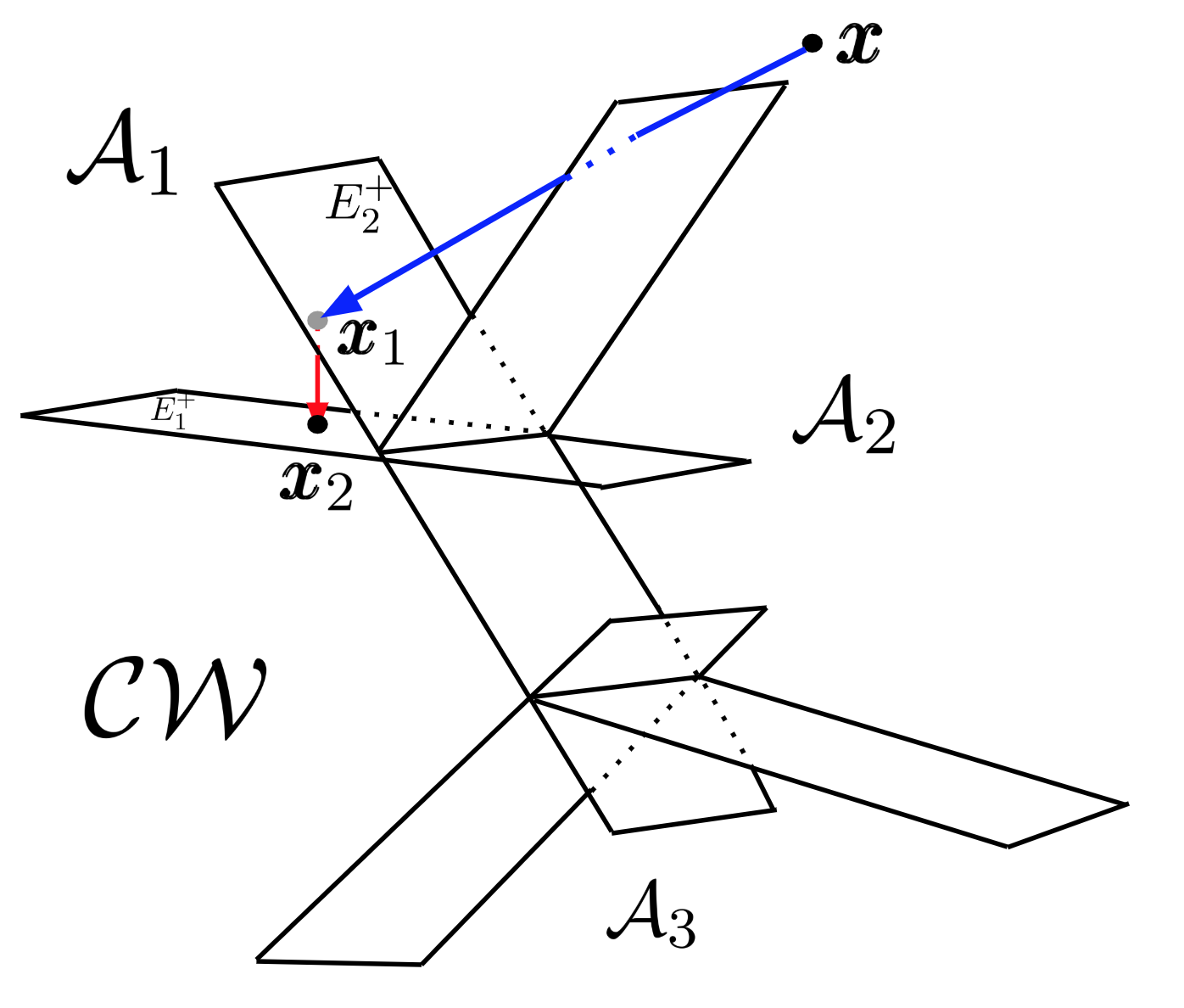
Figure 7: Sequential jumps at time $0$

Algorithm $\bf 1$ describes how players sequentially jump to $\overline{\mathcal{CW}}$. In order to show that this algorithm is well defined, one needs to make sure that such jumps stop in finite steps or converge to a limit point on $\hat{\boldsymbol{x}}\in\partial\overline{\mathcal{CW}}$, and that the total distance of such sequential jumps is bounded. The detailed argument is given in Appendix B, with the illustration of Figure 7.

Algorithm 1 Policy: Sequential jumps when $\boldsymbol{x}\notin\overline{\mathcal{CW}}$.

1:procedure Sequential($\boldsymbol{x}$)

2:     Define mapping,

$$\begin{aligned} i&=\pi(\boldsymbol{y})\quad\mbox{when}\quad\boldsymbol{y}\in\mathcal{A}_{i},\\ \emptyset&=\pi(\boldsymbol{y})\quad\mbox{when}\quad\boldsymbol{y}\in\overline{\mathcal{CW}}.\end{aligned}$$ (2.27)

3:     $\hat{\boldsymbol{x}}\leftarrow\boldsymbol{x}$, $k\leftarrow 0$

4:     while $\pi(\hat{\boldsymbol{x}})\not=\emptyset$ do

5:         $\lambda^{*}\leftarrow\arg\min\left\{\lambda>0\ \left|\ \hat{\boldsymbol{x}}+\lambda\boldsymbol{e}_{\pi(\hat{\boldsymbol{x}})}\in\partial E^{-}_{\pi(\hat{\boldsymbol{x}})}\mbox{ or }\hat{\boldsymbol{x}}-\lambda\boldsymbol{e}_{\pi(\hat{\boldsymbol{x}})}\in\partial E^{+}_{\pi(\hat{\boldsymbol{x}})}\right.\right\}$ $\triangleright$ $e_{j}$ is a unit vector in $\mathbb{R}^{N}$ with $j$th component to be 1

6:         if $\hat{\boldsymbol{x}}+{\lambda^{*}}\boldsymbol{e}_{\pi(\hat{\boldsymbol{x}})}\in\partial E^{-}_{\pi(\hat{\boldsymbol{x}})}$ then

7:              $\boldsymbol{\nu}_{0}\leftarrow\boldsymbol{e}_{\pi(\hat{\boldsymbol{x}})}$

8:         else

9:              $\boldsymbol{\nu}_{0}\leftarrow-\boldsymbol{e}_{\pi(\hat{\boldsymbol{x}})}$          

10:         $\hat{\boldsymbol{x}}\leftarrow\hat{\boldsymbol{x}}+\lambda^{*}\boldsymbol{\nu_{0}}$ $\triangleright$ Control of player $\pi(\hat{\boldsymbol{x}})$

11:         $\boldsymbol{x}_{k}\leftarrow\hat{\boldsymbol{x}}$

12:         $k\leftarrow k+1$      

13:     return $\hat{\boldsymbol{x}},\{\boldsymbol{x}_{k}\}$$\triangleright$ $\hat{\boldsymbol{x}}\in\partial{\mathcal{CW}}$

Note that this algorithm gives an $\epsilon$-NE in finite steps. In the case that the starting point is in the intersection of faces, a small perturbation in the algorithm and in the NE value will recover the case of $\boldsymbol{x}\in\mathcal{CW}$. In summary,

Theorem 5 (NE for the $N$-player game).

Under Assumption A1, a Markovian NE for game (2.2) is given by

$$\begin{aligned} \xi_{t}^{i*,+}&=\Delta_{0}^{i*,+}+\int_{0}^{t}\textbf{1}_{\left\{\boldsymbol{X}_{s}^{*}\in F_{i}\right\}}d\eta^{i}(s),\\ \xi_{t}^{i*,-}&=\Delta_{0}^{i*,-}+\int_{0}^{t}\textbf{1}_{\left\{\boldsymbol{X}_{s}^{*}\in F_{i+N}\right\}}d\eta^{i+N}(s),\end{aligned}$$ (2.28)

where $\mathcal{CW}$ is given in (2.6), $\boldsymbol{X}_{t}^{*}$ is the controlled dynamic with $\boldsymbol{X}_{0}^{*}=\hat{\boldsymbol{x}}=\boldsymbol{x}+\boldsymbol{\Delta_{0}}^{*,+}-\boldsymbol{\Delta_{0}}^{*,-}\in\overline{\mathcal{CW}},$ with $\eta^{j}(t)=\int_{0}^{t}\textbf{1}_{\{\boldsymbol{X}_{s}^{*}\in F_{j}\}}d\eta^{j}(s)$ and $\eta^{j}(0)=0$ $(j=1,2,\cdots,2N)$, the jumps at time $0$ are

$$\begin{aligned} \Delta_{0}^{i*,+}&=&\sum_{k}\textbf{1}_{\left\{\boldsymbol{x}_{k}\in\mathcal{A}_{i}\right\}}\left(x_{k+1}^{i}-x_{k}^{i}\right)_{+},\\ \Delta_{0}^{i*,-}&=&\sum_{k}\textbf{1}_{\left\{\boldsymbol{x}_{k}\in\mathcal{A}_{i}\right\}}\left(x^{i}_{k}-x^{i}_{k+1}\right)_{+},\end{aligned}$$ (2.29)

with $\{\boldsymbol{x}_{k}\}$ the sequence of jumps prescribed by Algorithm 1.

The corresponding NE value $v^{i}(x^{1},\ldots,x^{N}):=J^{i}(x^{1},\ldots,x^{N};\boldsymbol{\xi}^{*})$ is given by

$$v^{i}(x^{1},\ldots,x^{N})=\left\{\begin{array}[]{ll}v^{i}\left(x^{1},\ldots,x^{j-1},\frac{\sum_{k\neq j}x^{k}}{N-1}-c_{N},x^{j+1},\ldots,x^{N}\right),\\ \hskip 160.0pt\boldsymbol{x}\in E_{j}^{-}\cap\mathcal{A}_{j},\mbox{ for any }j\neq i,\\ v^{i}\left(x^{1},\ldots,\frac{\sum_{j\neq i}x^{j}}{N-1}-c_{N},\ldots,x^{N}\right)-c_{N}-x^{i}+\frac{\sum_{j\neq i}x^{j}}{N-1},\\ \hskip 230.0pt\boldsymbol{x}\in E_{i}^{-}\cap\overline{\mathcal{W}}_{-i},\\ -\frac{p_{N}^{\prime\prime}(c_{N})\cosh\left(\sqrt{\frac{2(N-1)\alpha}{N}}\left(x^{i}-\frac{\sum_{j\neq i}x^{j}}{N-1}\right)\right)}{\frac{2(N-1)\alpha}{N}\cosh\left(c_{N}\sqrt{\frac{2(N-1)\alpha}{N}}\right)}+p_{N}\left(x^{i}-\frac{\sum_{j\neq i}x^{j}}{N-1}\right),\\ \hskip 190.0pt\boldsymbol{x}\in(E_{i}^{-}\cup E_{i}^{+})^{c}\cap\overline{\mathcal{W}}_{-i},\\ x^{i}-\frac{\sum_{j\neq i}x^{j}}{N-1}-c_{N}+v^{i}\left(x^{1},\ldots,\frac{\sum_{j\neq i}x^{j}}{N-1}+c_{N},\ldots,x^{N}\right),\\ \hskip 230.0pt\boldsymbol{x}\in E_{i}^{+}\cap\overline{\mathcal{W}}_{-i},\\ v^{i}\left(x^{1},\ldots,x^{j-1},\frac{\sum_{k\neq j}x^{k}}{N-1}+c_{N},x^{j+1},\ldots,x^{N}\right),\\ \hskip 160.0pt\boldsymbol{x}\in E_{j}^{+}\cap\mathcal{A}_{j},\mbox{ for any }j\neq i.\end{array}\right.$$ (2.40)

Here $E_{i}^{+}$, $E_{i}^{-}$ are given in (2.15), and $\mathcal{A}_{i}$ and $\mathcal{W}_{i}$ defined in (2.14).

Figure (2(a)) shows the region partition when $N=3$. $\mathcal{CW}$, the unbounded polytope, is surrounded by the action regions $\mathcal{A}_{i}$, $i=1,2,3$. Figure (2(b)) shows the action region $\mathcal{A}_{1}$ of player one and the common waiting region $\mathcal{CW}$ of all players.

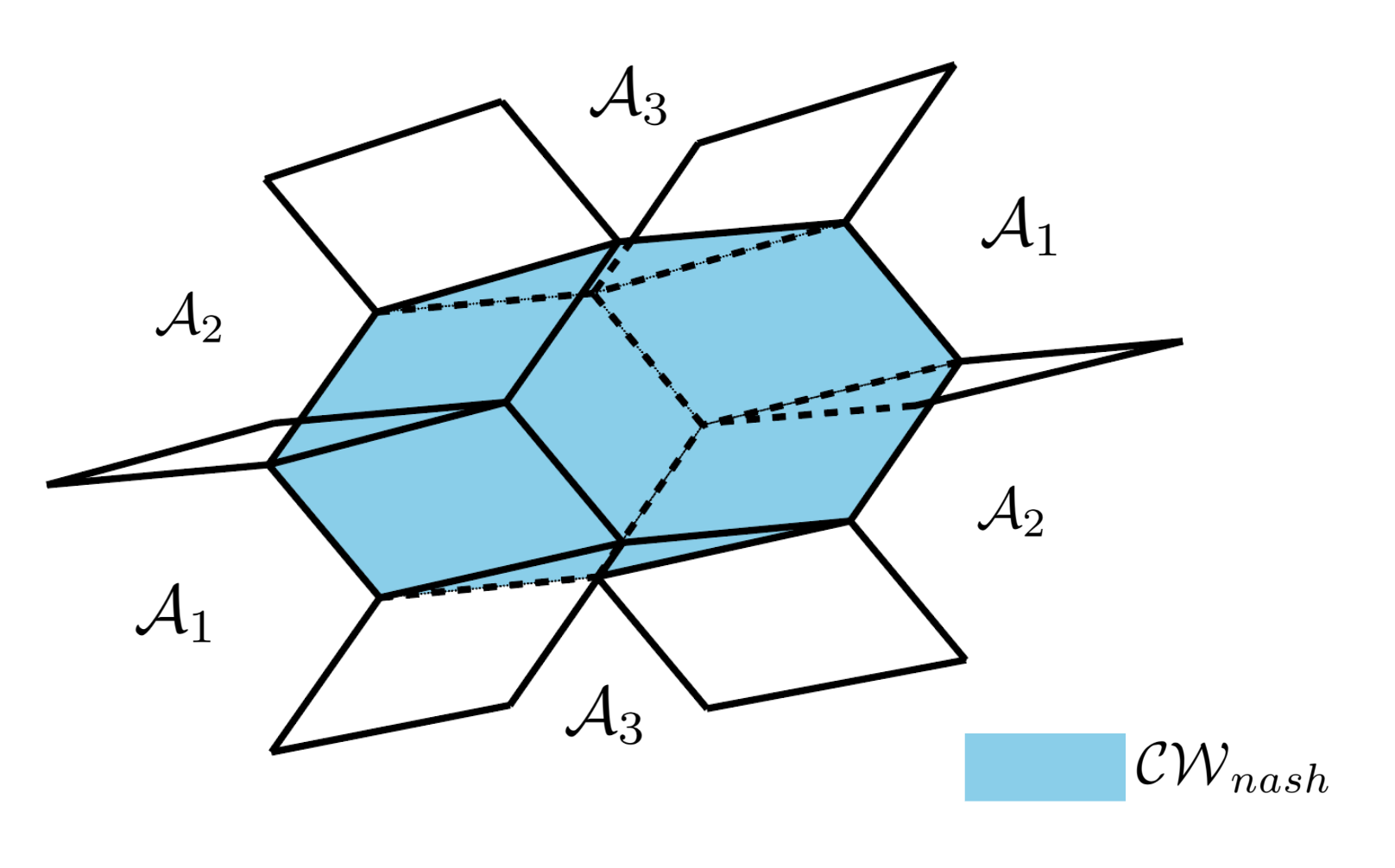
(a) $\mathcal{CW}$ and $\mathcal{A}_{i}$ ($i=1,2,3$)

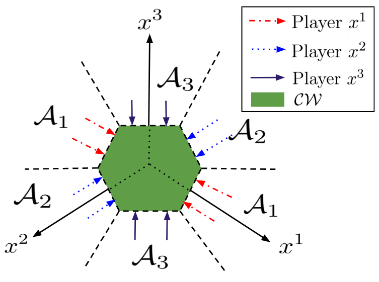
(b) $\mathcal{A}_{1}$ and $\mathcal{W}_{1}$,
a bird’s-eye view from $(1,1,1)$
to $(0,0,0)$

Figure 2: Region partition when $N=3$

3 MFG for the Fuel Follower Problem

Take $N$ identical, rational, and interchangeable players, whose initial positions are random in $\mathbb{R}^{N}$. Let $N\rightarrow\infty$, the MFG for the fuel follower problem is to find a closed-loop control in feedback form of

$$\begin{aligned} v(x)=&\inf_{(\xi^{+},\xi^{-})\in\mathcal{U}_{\infty}}J_{(\infty)}(x;\xi_{t}^{+},\xi_{t}^{-})\\ =&\inf_{(\xi^{+},\xi^{-})\in\mathcal{U}_{\infty}}\mathbb{E}\int_{0}^{\infty}e^{-\alpha t}\left[h(X_{t}-m_{t})dt+d\check{\xi_{t}}|X_{0-}=x\right],\\ \mbox{such that}&\qquad dX_{t}=dB_{t}+d\xi_{t}^{+}-d\xi_{t}^{-},\\ &\hskip 20.0pt\ \ X_{0-}\sim\mu_{0-},\,\,m_{0-}=\int x\mu_{0-}(dx),\end{aligned}$$ (3.1)

where $\mu_{t}=\lim_{N\rightarrow\infty}\frac{\sum_{i=1}^{N}\textbf{1}_{\{X^{i}_{t}\}}}{N}$ is the distribution of $X_{t}$ and $m_{t}=\lim_{N\rightarrow\infty}\frac{\sum_{i=1}^{N}X^{i}_{t}}{N}=\int x\mu_{t}(dx)$ is the mean position of the population at time $t$, with $\mu_{0-}$ symmetric around $m_{0-}$.

Note that one could write an alternative MFG formulation with

$$\tilde{v}(\mu_{0-}):=\inf_{(\xi^{+},\xi^{-})\in\mathcal{U}_{\infty}}\mathbb{E}\int_{0}^{\infty}e^{-\alpha t}\left[h(X_{t}-m_{t})dt+d\check{\xi_{t}}\right].$$

$v(x)$ defined in (3.1) can be viewed as $\tilde{v}(\mu_{0-}|X_{0-}=x)$ with $X_{0-}=x$ as some sample drawn from $\mu_{0-}$. Clearly $\tilde{v}(\mu_{0-})$ can be solved by analyzing $v(x)$ as $\tilde{v}(\mu_{0-})=\mathbb{E}_{\mu_{0-}}[v(X_{0-})]$. This connection is also explored in Section 2.2.2 of [35].

The admissible control set for MFG is

$$\begin{aligned} \mathcal{U}_{\infty}=&\left\{(\xi_{t}^{+},\xi_{t}^{-})\>\lvert\>\xi_{t}^{+}\mbox{ and }\xi_{t}^{-}\mbox{ are }\mathcal{F}_{t}^{(X_{t-},m_{t-})}\mbox{-progressively measurable, c\`{a}dl\`{a}g, non-decreasing,}\right.\\ &\hskip 50.0pt\left.{}\mbox{ with }\mathbb{E}\left[\int_{0}^{\infty}e^{-\alpha t}d\xi_{t}^{+}\right]<\infty,\enspace\mathbb{E}\left[\int_{0}^{\infty}e^{-\alpha t}d\xi_{t}^{-}\right]<\infty,\enspace\xi_{0-}^{+}=0,\enspace\xi_{0-}^{-}=0\right\}.\end{aligned}$$

3.1 NE Solution to the MFG

Definition 6 (NE to MFG (3.1)).

An NE to the MFG (3.1) is a pair of Markovian control $(\xi_{t}^{*,+},\xi_{t}^{*,-})_{t\geq 0}$ and a mean function $\{m^{*}_{t}\}_{t\geq 0}$ such that

• ${v}^{*}(x)=J_{(\infty)}\left(x;\xi^{*,+},\xi^{*,-}|\{\mu^{*}_{t}\}_{t\geq 0}\right)=\min_{\xi\in\mathcal{U}_{\infty}}J_{(\infty)}\left(x;\xi^{+},\xi^{-}|\{\mu^{*}_{t}\}_{t\geq 0}\right)$,

• $P_{X^{*}_{t}}=\mu_{t}^{*}$, and $m_{t}^{*}=\int xP_{X^{*}_{t}}(dx)$ is the mean function of $X_{t}^{*}$ where $X_{t}^{*}$ is the controlled dynamic under $(\xi_{t}^{*,+},\xi_{t}^{*,-})_{t\geq 0}$.

${v}^{*}(x)$ is called the NE value of the MFG associated with ${\xi}^{*}$.

Theorem 7 (NE to MFG (3.1)).

There exists an NE to the MFG (3.1),

$$\begin{aligned} \xi^{*,+}_{t}&=&\max\left\{0,\max_{0\leq u\leq t}\{{m_{0-}}-x-B_{u}+\xi_{u}^{*,-}-c\}\right\},\\ \xi^{*,-}_{t}&=&\max\left\{0,\max_{0\leq u\leq t}\{x-{m_{0-}}+B_{u}+\xi_{u}^{*,+}-c\}\right\},\end{aligned}$$ (3.2)

and the corresponding NE value is

$$v^{*}(x)=\left\{\begin{array}[]{ll}-\frac{p_{1}^{\prime\prime}(c\sqrt{2\alpha})\cosh\left(x\sqrt{2\alpha}\right)}{2\alpha\cosh\left(c\sqrt{2\alpha}\right)}+p_{1}(x-{m_{0-}}),&{m_{0-}}\leq x\leq{m_{0-}}+c,\\ v({m_{0-}}+c)+(x-{m_{0-}}-c),&x\geq{m_{0-}}+c,\\ v({m_{0-}}-x),&x<{m_{0-}},\end{array}\right.$$ (3.6)

where c is the solution to (2.4).

The proof consists of three steps.

Step 1: Stochastic control problem.

Take the $M_{1}$ topology for the Skorokhod space $\mathcal{D}([0,\infty))$ with a Wasserstein distance $W_{1}$([40, 19]). Fix a mean field measure $\{\mu_{t}\}_{t\geq 0}\in\mathcal{P}_{1}(\mathcal{D}([0,\infty)))$, with $m_{t}=\int x\mu_{t}(dx)$ and $\mathcal{P}_{1}$ the class of all probability measures with finite moment of first order. Then (3.1) becomes the following time-dependent and state-dependent singular control problem,

$$\begin{aligned} \hat{v}(s,x)&=\inf_{{\xi}\in\mathcal{U}_{\infty}}\mathbb{E}\int_{s}^{\infty}e^{-\alpha(t-s)}\left[h(X_{t}-m_{t})dt+d\xi_{t}^{+}+d\xi_{t}^{-}\right]\\ \mbox{ such that }&\hskip 20.0ptdX_{t}=dB_{t}+d\xi_{t}^{+}-d\xi_{t}^{-},\,X_{s-}=x,\,m_{s-}=m.\end{aligned}$$ (3.7)

The corresponding HJB equation for $\hat{v}(s,x)$ is

$$\begin{aligned} &&\max\left\{\alpha\hat{v}(s,x)-\hat{v}_{t}(s,x)-\frac{1}{2}\hat{v}_{xx}(s,x)-h(x-m),-1+\hat{v}_{x}(s,x),-1-\hat{v}_{x}(s,x)\right\}=0.\end{aligned}$$ (3.8)

Note that (3.8) is a parabolic equation because of $\mu_{t}$ despite the infinite horizon. This is different from the elliptic equation (2.3).

We will show that $\hat{v}(s,x)$ in (3.7) is a viscosity solution to HJB equation (3.8).

First, under a fixed $\{\mu_{t}\}_{t\geq 0}$, the following dynamic programming principle holds.

Dynamic programming principle (DPP).

For all $(s,x)\in\mathbb{R}^{+}\times\mathbb{R}$,

$$\hat{v}(s,x)=\inf_{\xi\in\mathcal{U}_{\infty}}\mathbb{E}\left[\int_{s}^{\theta}e^{-\alpha(t-s)}\left(h(X_{t}-m_{t})dt+d\check{\xi}_{t}\right)+{e}^{-\alpha(\theta-s)}v(\theta,X_{\theta})\right]$$ (3.9)

for any $\theta\in\mathcal{T}$ and $\theta\geq s$, with $\mathcal{T}$ the set of all $\{\mathcal{F}^{{(X_{t},m_{t})}}\}_{t\geq 0}$-stopping times. Here, we adopt the convention that $e^{-\alpha\theta(\omega)}=0$ when $\theta(\omega)=\infty$. The proof of DPP (3.9) follows Guo and Pham [21] by extending the state space from $\mathbb{R}$ to $\mathbb{R}^{+}\times\mathbb{R}$.

Definition 8 (Viscosity solution).

$\hat{v}(t,x)$ is a continuous viscosity solution to (3.8) on $[0,\infty)\times\mathbb{R}$ if

• Viscosity super-solution: for any $(t_{0},x_{0})\in[0,\infty)\times\mathbb{R}$ and for any function $\phi(t_{0},x_{0})$ such that $(t_{0},x_{0})$ is a local minimum of $(\hat{v}-\phi)(t,x)$ with $\hat{v}(t_{0},x_{0})=\phi(t_{0},x_{0})$,

  $$\max\left\{\alpha\phi(t_{0},x_{0})-\phi_{t}(t_{0},x_{0})-\frac{1}{2}\phi_{x,x}(t_{0},x_{0})-h(x_{0}-m),-1+\phi_{x}(t_{0},x_{0}),-1-\phi_{x}(t_{0},x_{0})\right\}\geq 0.$$

• Viscosity sub-solution: for any $(t_{0},x_{0})\in[0,\infty)\times\mathbb{R}$ and for any function $\phi(t_{0},x_{0})$ such that $(t_{0},x_{0})$ is a local maximum of $(\hat{v}-\phi)(t,x)$ with $\hat{v}(t_{0},x_{0})=\phi(t_{0},x_{0})$,

  $$\max\left\{\alpha\phi(t_{0},x_{0})-\phi_{t}(t_{0},x_{0})-\frac{1}{2}\phi_{x,x}(t_{0},x_{0})-h(x_{0}-m),-1+\phi_{x}(t_{0},x_{0}),-1-\phi_{x}(t_{0},x_{0})\right\}\leq 0.$$

Proposition 9.

Assume that the value function $\hat{v}(t,x)$ of (3.7) is continuous with respect to $t$. Then $\hat{v}(t,x)$ is a continuous viscosity solution of the HJB equation (3.8) on $[s,\infty)\times\mathbb{R}$. Moreover, $\hat{v}(t,x)$ is convex and differentiable in $x$, and for any $x,y\in\mathbb{R}$,

$$\hat{v}(s,x)\leq\hat{v}(s,y)+|x-y|.$$ (3.10)

Proof.

Since $h$ is convex and the pay-off function $\mathbb{E}\left[\int_{s}^{\infty}e^{-\alpha(t-s)}h(X_{t}-m_{t})dt+d\xi_{t}^{+}+d\xi_{t}^{-}\right]$ in problem (3.7) is linear in control $(\xi^{+},\xi^{-})$, the value function $\hat{v}(s,x)$ is convex in $x$. Since $\hat{v}(s,x)$ is finite and convex on $(-\infty,\infty)$, it is continuous in $x$. Moreover, consider a special control,

$$\xi_{t}^{+}-\xi_{t}^{-}=\left\{\begin{array}[]{ll}0,\quad t=s,\\ y-x,\quad t\geq s,\end{array}\right.$$ (3.13)

clearly $\hat{v}(s,x)\leq\hat{v}(s,y)+|y-x|$ .

We now prove that the value function is a viscosity solution of (3.8).

• Step A: Viscosity sub-solution.
  For some $(t_{0},x_{0})\in\mathbb{R}^{+}\times\mathbb{R}$ and $\phi\in\mathcal{C}^{1,2}(\mathbb{R}^{+}\times\mathbb{R})$ such that $\hat{v}(t_{0},x_{0})=\phi(t_{0},x_{0})$ and $\phi(t_{0},x_{0})\geq\hat{v}(t_{0},x_{0})$ for $(t,x)\in B_{\epsilon}(t_{0},x_{0})$. That is, $\hat{v}-\phi$ has local maximum at $(t_{0},x_{0})$. Consider the following admissible control

  $$\xi_{t}^{+}=\left\{\begin{array}[]{ll}0,\quad t=t_{0},\\ \eta_{1},\quad t\geq t_{0},\end{array}\right.$$ (3.16)

  $$\xi_{t}^{-}=\left\{\begin{array}[]{ll}0,\quad t=t_{0},\\ \eta_{2},\quad t\geq t_{0},\end{array}\right.$$ (3.19)

  where $0\leq\eta_{1},\eta_{2}\leq\epsilon$. Define the exit time

  $$\tau_{\epsilon}=\inf\left\{t\geq t_{0},X_{t}\notin\bar{B}_{\epsilon}(t_{0},x_{0})\right\}.$$ (3.20)

  Notice that $X$ has at most one jump at $t=t_{0}$ and is continuous on $[t_{0},t_{0}+\tau_{\epsilon})$. By the DPP,

  $$\begin{aligned} \phi(t_{0},x_{0})=\hat{v}(t_{0},x_{0})&\leq&\mathbb{E}\int_{t_{0}}^{t_{0}+\tau_{\epsilon}\wedge\delta}e^{-\alpha(t-t_{0})}\left[h(X_{t}-m_{t})dt+d\xi_{t}^{+}+d\xi_{t}^{-}\right]\\ &\enspace&+\enspace\mathbb{E}\left[e^{-\alpha(\tau_{\epsilon}\wedge\delta)}\phi(t_{0}+\tau_{\epsilon}\wedge\delta,X_{t_{0}+\tau_{\epsilon}\wedge\delta})\right].\end{aligned}$$ (3.21)

  By Itô’s lemma,

  $$\begin{aligned} &\mathbb{E}[e^{-\alpha(\tau_{\epsilon}\wedge\delta)}\phi(t_{0}+\tau_{\epsilon}\wedge\delta,X_{t_{0}+\tau_{\epsilon}\wedge\delta})]\\ =\phi(t_{0},x_{0})&+\mathbb{E}\left[\int_{t_{0}}^{t_{0}+\tau_{\epsilon}\wedge\delta}e^{-\alpha(t-t_{0})}(-\alpha\phi+\phi_{t}+\frac{1}{2}\phi_{x,x})(t,X_{t})dt\right]\\ \quad&+\enspace\mathbb{E}\left[\sum_{t_{0}\leq t\leq\tau_{\epsilon}\wedge\delta}e^{-\alpha t}(\phi(t,X_{t})-\phi(t,X_{t-}))\right].\end{aligned}$$ (3.22)

  Combining (3.21) and (3.22),

  $$\begin{aligned} &\mathbb{E}\left[\int_{t_{0}}^{t_{0}+\tau_{\epsilon}\wedge\delta}e^{-\alpha(t-t_{0})}(\alpha\phi-\phi_{t}-\frac{1}{2}\phi_{x,x}-h)(t,X_{t})dt\right]\\ -&\mathbb{E}\left[\int_{t_{0}}^{t_{0}+\tau_{\epsilon}\wedge\delta}e^{-\alpha(t-t_{0})}(d\xi_{t}^{+}+d\xi_{t}^{-})\right]\\ -&\mathbb{E}\left[\sum_{t_{0}\leq t\leq\tau_{\epsilon}\wedge\delta}e^{-\alpha t}(\phi(t,X_{t})-\phi(t,X_{t-}))\right]\leq 0.\end{aligned}$$ (3.23)

  Now, setting $\eta_{1}=\eta_{2}=0$ and letting $\delta\rightarrow 0$ leads to $\alpha\phi-\phi_{t}-\frac{1}{2}\phi_{x,x}-h\leq 0$.

  Next, let $\eta_{2}=0$, and note that $\xi^{+}_{t}$ and $X_{t}$ only jump at time $t_{0}$ with a size $\eta_{1}$, therefore

  $$\mathbb{E}\left[\int_{t_{0}}^{t_{0}+\tau_{\epsilon}\wedge\delta}e^{-\alpha(t-t_{0})}(\alpha\phi-\phi_{t}-\frac{1}{2}\phi_{x,x}-h)(t,X_{t})dt\right]-\eta_{1}-\phi(t_{0},x_{0}+\eta_{1})+\phi(t_{0},x_{0})\leq 0.$$

  Now, taking $\delta\rightarrow 0$, dividing by $\eta_{1}$, and letting $\eta_{1}\rightarrow 0$ yields $-1-\phi_{x}\leq 0$. Similarly, $-1+\phi_{x}\leq 0$. That is, $\phi$ is the sub-solution to (3.8), so that

  $$\max\left\{\alpha\phi(t_{0},x_{0})-\phi_{t}(t_{0},x_{0})-\frac{1}{2}\phi_{x,x}(t_{0},x_{0})-h(x_{0}-m),-1-\phi_{x}(t_{0},x_{0}),-1+\phi_{x}(t_{0},x_{0})\right\}\leq 0.$$

• Step B: Viscosity Super-solution.
  This is established by a contradiction argument. Suppose otherwise, then there exists $(t_{0},x_{0})$, $\epsilon,\delta>0$ $\phi\in C^{1,2}(\mathbb{R}^{+}\times\mathbb{R})$ such that for any $(t,x)\in\bar{B}_{\epsilon}(t_{0},x_{0})$,

  $$\begin{cases}\alpha\phi-\frac{1}{2}\phi_{x,x}-h(x-m)-\phi_{t}\leq-\delta,\\ -1+\delta\leq\phi_{x}\leq 1-\delta.\end{cases}$$ (3.24)

  Given any admissible control $(\xi^{+},\xi^{-})\in\mathcal{U_{\infty}}$, consider an exit time $\tau_{\epsilon}=\inf\{t\geq 0,X_{t+t_{0}}\notin\bar{B}_{\epsilon}(t_{0},x_{0})\}$, and apply Itô’s lemma to $e^{-\alpha t}\phi(t,X_{t})$,

  $$\begin{aligned} \mathbb{E}\left[e^{-\alpha\tau_{\epsilon}}\phi(t_{0}+\tau_{\epsilon},X_{t_{0}+\tau_{\epsilon}})\right]&=\phi(t_{0},x_{0})+\mathbb{E}\left[\int_{t_{0}}^{t_{0}+\tau_{\epsilon}}e^{-\alpha(t-t_{0})}(-\alpha\phi+\phi_{t}+\frac{1}{2}\phi_{x,x})(t,X_{t})dt\right]\\ &\enspace\enspace+\enspace\mathbb{E}\left[\sum_{t_{0}\leq t\leq\tau_{\epsilon}}e^{-\alpha t}(\phi(t,X_{t})-\phi(t,X_{t-}))\right]\\ &\enspace\enspace+\enspace\mathbb{E}\left[\int_{t_{0}}^{t_{0}+\tau_{\epsilon}}e^{-\alpha t}\phi^{\prime}(t,X_{t})\left(\left(d\xi_{t}^{+}\right)^{c}+\left(d\xi_{t}^{-}\right)^{c}\right)\right].\end{aligned}$$

  Notice that for any $t_{0}\leq t\leq t_{0}+\tau_{\epsilon}$, $(t,X_{t})\in\bar{B}_{\epsilon}(t_{0},x_{0})$. By the Taylor expansion and $\Delta X_{t}=\Delta\xi^{+}_{t}-\Delta\xi^{-}_{t}$, clearly for any $0\leq t<\tau_{\epsilon}$:

  $$\phi(t,X_{t})-\phi(t,X_{t-}) = \Delta X_{t}\int_{0}^{1}\phi_{x}(t,X_{t}+z\Delta X_{t})dz$$ (3.25)

  $$\geq (-1+\delta)(\Delta\xi_{t}^{+}+\Delta\xi_{t}^{-}).$$

  Thus,

  $$\begin{aligned} &\mathbb{E}[e^{-\alpha\tau_{\epsilon}}\phi(t_{0}+\tau_{\epsilon},X_{t_{0}+\tau_{\epsilon}-})]\\ \geq\phi(t_{0},x_{0})&+\mathbb{E}\left[\int_{t_{0}}^{t_{0}+\tau_{\epsilon}}e^{-\alpha(t-t_{0})}(-h+\delta)(t,X_{t})dt\right]\\ \quad&+(\delta-1)\mathbb{E}\left[\int_{t_{0}}^{t_{0}+\tau_{\epsilon}-}e^{-\alpha(t-t_{0})}(d\xi_{t}^{+}+d\xi_{t}^{-})\right]\\ =\phi(t_{0},x_{0})&+\mathbb{E}\left[\int_{t_{0}}^{t_{0}+\tau_{\epsilon}}e^{-\alpha(t-t_{0})}\left(-h(X_{t}-m_{t})dt-d\xi_{t}^{+}-d\xi_{t}^{-}\right)\right]\\ \quad&+\mathbb{E}\left[e^{-\alpha\tau_{\epsilon}}(\Delta\xi_{t_{0}+\tau_{\epsilon}}^{+}+\Delta\xi_{t_{0}+\tau_{\epsilon}}^{-})]+\delta\mathbb{E}[\int_{t_{0}}^{t_{0}+\tau_{\epsilon}}e^{-\alpha t}dt\right]\\ \quad&+\delta\mathbb{E}\left[\int_{t_{0}}^{t_{0}+\tau_{\epsilon}-}e^{-\alpha(t-t_{0})}(d\xi_{t}^{+}+d\xi_{t}^{-})\right].\end{aligned}$$ (3.26)

  By definition of $\tau_{\epsilon}$, $(t_{0}+\tau_{\epsilon}-,X_{t_{0}+\tau_{\epsilon}-})\in\bar{B}_{\epsilon}(t_{0},x_{0})$ and $(t_{0}+\tau_{\epsilon},X_{t_{0}+\tau_{\epsilon}})$ is either on the boundary $\partial{B}_{\epsilon}(t_{0},x_{0})$ or out of $\bar{B}_{\epsilon}(t_{0},x_{0})$. However, there exists some random variable $\alpha\in[0,1]$ such that,

  $$x_{\alpha} = X_{t_{0}+\tau_{\epsilon}-}+\alpha\Delta X_{t_{0}+\tau_{\epsilon}}$$

  $$= X_{t_{0}+\tau_{\epsilon}-}+\alpha(\Delta\xi^{+}_{t_{0}+\tau_{\epsilon}}-\Delta\xi^{-}_{t_{0}+\tau_{\epsilon}})\in\partial B_{\epsilon}(t_{0},x_{0}).$$

  Similar as in (3.25), we have

  $$\begin{aligned} \phi(t_{0}+\tau_{\epsilon},x_{\alpha})-\phi(t_{0}+\tau_{\epsilon},X_{t_{0}+\tau_{\epsilon}-})\geq\alpha(-1+\delta)(\Delta\xi_{t_{0}+\tau_{\epsilon}}^{+}+\Delta\xi_{t_{0}+\tau_{\epsilon}}^{-}).\end{aligned}$$ (3.27)

  Notice that $X_{t_{0}+\tau_{\epsilon}}=x_{\alpha}+(1-\alpha)(\Delta\xi_{t_{0}+\tau_{\epsilon}}^{+}-\Delta\xi_{t_{0}+\tau_{\epsilon}}^{-})$, and from (3.10),

  $$\hat{v}(t_{0}+\tau_{\epsilon},x_{\alpha})\leq\hat{v}(t_{0}+\tau_{\epsilon},X_{t_{0}+\tau_{\epsilon}})+(1-\alpha)(\Delta\xi_{t_{0}+\tau_{\epsilon}}^{+}+\Delta\xi_{t_{0}+\tau_{\epsilon}}^{-}).$$ (3.28)

  Recalling $\phi(t_{0}+\tau_{\epsilon},x_{\alpha})\leq\hat{v}(t_{0}+\tau_{\epsilon},x_{\alpha})$, inequalities (3.27) and (3.28) imply

  $$\phi(t_{0}+\tau_{\epsilon},X_{t_{0}+\tau_{\epsilon}-})\leq\hat{v}(t_{0}+\tau_{\epsilon},X_{t_{0}+\tau_{\epsilon}})+(1-\alpha\delta)(\Delta\xi_{t_{0}+\tau_{\epsilon}}^{+}+\Delta\xi_{t_{0}+\tau_{\epsilon}}^{-}).$$

  Plugging the above inequality into (3.26), by $\phi(t_{0},x_{0})=\hat{v}(t_{0},x_{0})$,

  $$\begin{aligned} \mathbb{E}e^{-\alpha\tau_{\epsilon}}&\left[\int_{t_{0}}^{t_{0}+\tau_{\epsilon}}\left(h(X_{t}-m_{t})dt+d\xi_{t}^{+}+d\xi_{t}^{-}\right)+\hat{v}(t_{0}+\tau_{\epsilon},X_{t_{0}+\tau_{\epsilon}})\right]\\ \geq\hat{v}(t_{0},x_{0})&+\alpha\delta\mathbb{E}\left[e^{-\alpha\tau_{\epsilon}}(\Delta\xi_{t_{0}+\tau_{\epsilon}}^{+}+\Delta\xi_{t_{0}+\tau_{\epsilon}}^{-})\right]\\ &+\delta\mathbb{E}\left[\int_{t_{0}}^{t_{0}+\tau_{\epsilon}}e^{-\alpha t}dt\right]+\delta\mathbb{E}\left[\int_{t_{0}}^{t_{0}+\tau_{\epsilon}-}e^{-\alpha(t-t_{0})}(d\xi_{t}^{+}+d\xi_{t}^{-})\right].\end{aligned}$$ (3.29)

  There exists a constant $g_{0}>0$ such that for any $(\xi^{+},\xi^{-})\in\mathcal{U}_{\infty}$,

  $$\alpha\mathbb{E}\left[e^{-\alpha\tau_{\epsilon}}(\Delta\xi_{t_{0}+\tau_{\epsilon}}^{+}+\Delta\xi_{t_{0}+\tau_{\epsilon}}^{-})\right]+\mathbb{E}\left[\int_{t_{0}}^{t_{0}+\tau_{\epsilon}}e^{-\alpha t}dt\right]+\mathbb{E}\left[\int_{t_{0}}^{t_{0}+\tau_{\epsilon}-}e^{-\alpha(t-t_{0})}(d\xi_{t}^{+}+d\xi_{t}^{-})\right]\geq g_{0}.$$

  Finally, taking the infimum over all admissible controls $(\xi^{+},\xi^{-})\in\mathcal{U}_{\infty}$ in (3.29) suggests

  $$\hat{v}(t_{0},x_{0})\geq\hat{v}(t_{0},x_{0})+\delta g_{0},$$ (3.30)

  which is a contradiction.

The differentiability with respect to $x$ can be proved using the convexity of the value function $\hat{v}(s,x)$ to (3.8). Since $\hat{v}(s,x)$ is convex, the left and right derivatives with respect to $x$, $\hat{v}_{x-}(t,x)$ and $\hat{v}_{x+}(t,x)$ exist for any $t\geq s$ and $x\in\mathbb{R}$. Also, $\hat{v}_{x-}(t,x)\leq\hat{v}_{x+}(t,x)$ by convexity. We argue by contradiction and suppose there exists $x_{0}\in\mathbb{R}$ and $t_{0}\geq 0$ such that $\hat{v}_{x-}(t_{0},x_{0})<\hat{v}_{x+}(t_{0},x_{0})$. Fix some $q$ in $(\hat{v}_{x-}(t_{0},x_{0}),\hat{v}_{x+}(t_{0},x_{0}))$ and consider the test function

$$\phi_{\epsilon}(t,x)=\hat{v}(t_{0},x_{0})+q(x-x_{0})-\frac{1}{2\epsilon}(x-x_{0})^{2}-\frac{1}{2\epsilon}(t-t_{0})^{2},$$

with $\epsilon>0$. Then $(t_{0},x_{0})$ is a local minimum of $(\hat{v}-\phi_{\epsilon})(t,x)$ since $\hat{v}_{x-}(t_{0},x_{0})<q=\phi_{x}(t_{0},x_{0})<\hat{v}_{x+}(t_{0},x_{0})$ and $\phi_{t}(t_{0},x_{0})=0$. Hence $\phi$ is a viscosity super-solution by definition. That is,

$$\max\left\{\alpha\phi-\phi_{t}-\frac{1}{2}\phi_{x,x}-h(x_{0}-m),-1-\phi_{x},-1+\phi_{x}\right\}\geq 0,$$

which leads to $-\frac{1}{2\epsilon}+h(x_{0}-m)-\alpha\phi(t_{0},x_{0})\geq 0$. Taking $\epsilon>0$ sufficiently small leads to a contradiction. ∎

Proposition 10 (Optimal Control).

Assume A1 and assume that $\hat{v}_{t}(t,x)$ is continuous with respect to $t$, the optimal control to (3.7) under a fixed $\{\mu_{t}\}_{t\geq 0}\in\mathcal{P}_{1}(\mathcal{D}([0,\infty)))$ is of the form

$$d\hat{\xi}_{t}=\left\{\begin{array}[]{ll}m_{t}+c_{t}-x,&\hat{v}_{x}(t,x)=1,\\ 0,&|\hat{v}_{x}(t,x)|<1,\\ m_{t}-c_{t}-x,&\hat{v}_{x}(t,x)=-1,\end{array}\right.$$ (3.34)

where $t\geq 0$, $m_{t}=\int x\mu_{t}(dx)$, and $c_{t}=\inf\{x\>\lvert\>\hat{v}_{x}(t,x)=1\}-m_{t}=-\sup\{x\>\lvert\>\hat{v}_{x}(t,x)=-1\}+m_{t}$.

Proof.

By Proposition 9, $\hat{v}(t,x)$ is convex and differentiable in $x$, hence for any fixed $t\in[0,\infty)$, $c^{1}_{t}:=\inf\{x\>\lvert\>\hat{v}_{x}(t,x)=1\}-m_{t}$ and $c^{2}_{t}:=-\sup\{x\>\lvert\>\hat{v}_{x}(t,x)=-1\}+m_{t}$ exist. By the symmetry of Problem (3.1) under a fixed $\{m_{t}\}_{t\geq 0}$, $\hat{v}(t,m_{t}+\delta)=\hat{v}(t,m_{t}-\delta)$ and $\hat{v}_{x}(t,m_{t}+\delta)=-\hat{v}_{x}(t,m_{t}-\delta)$ for any fixed $t$ and any $\delta>0$, hence $c_{t}^{1}=c_{t}^{2}$, denoted as $c_{t}$.

Because $\hat{v}(t,x)$ is convex in $x$ and continuously differentiable in $x$ and $t$, one can apply the generalized Itô’s formula to $\hat{v}(t,x)$ with (3.34) and use a similar argument as the verification theorem in [29] to obtain the optimality of (3.34). ∎

Given the optimal control (3.34), define a mapping $\Gamma_{1}:\mathcal{P}_{1}(\mathcal{D}([0,\infty)))\rightarrow\mathcal{D}([0,\infty))$ such that

$$\Gamma_{1}\left(\{\mu_{t}\}_{t\geq 0}\right)=\{\hat{\xi}\ |\ \{\mu_{t}\}_{t\geq 0}\}_{t\geq 0}.$$

Step 2: Consistency.

Given Proposition 10 and a fixed flow $\{\mu_{t}\}_{t\geq 0}$, the optimal control $(\hat{\xi}_{t}^{+},\hat{\xi}_{t}^{-})$ to (3.8) is a bang-bang type and the controlled process $\hat{{X}}_{t}$ is a reflected Brownian motion with two time-dependent reflected boundaries $m_{t}+c_{t}$ and $m_{t}-c_{t}$. $m_{t}+c_{t},m_{t}-c_{t}\in\mathcal{C}([0,\infty])$ since $\hat{v}(t,x)$ is continuous and differentiable. By Theorem 2.6 in Burdzy, Kang, and Ramanan [9], there exists a unique solution, $\hat{{X}}_{t}$, to the SP with time varying domain $\{(t,x)\>\lvert\>m_{t}-c_{t}\leq x\leq c_{t}+m_{t}\}$ such that $\hat{{X}}_{t}$ is a càdàg process. Furthermore, by Theorem 2.9 in Burdy, Chen, and Sylvester [8], the Kolmogorov forward equation for $\hat{\mu}_{t}$ can be described as

$$\left\{\begin{array}[]{ll}p_{t}(t,x)-\frac{1}{2}p_{x,x}(t,x)=0,&\quad\mbox{ when }|x-m_{t}|<c_{t},\\ p_{x}(t,x)+2(\frac{\partial{{m}_{t}}}{\partial{t}}+\frac{\partial{{c}_{t}}}{\partial{t}})p(t,x)=0,&\quad\mbox{ when }x=m_{t}+c_{t},\\ p_{x}(t,x)-2(\frac{\partial{{m}_{t}}}{\partial{t}}-\frac{\partial{{c}_{t}}}{\partial{t}})p(t,x)=0,&\quad\mbox{ when }x=m_{t}-c_{t},\end{array}\right.$$ (3.38)

with the initial distribution $p(0,x)=\hat{\mu}_{0}\in\mathcal{P}_{1}(\mathbb{R})$, where

$$\hat{\mu}_{0}(x)=\left\{\begin{array}[]{ll}0,&x<m_{0-}-c_{0}\mbox{ or }x>m_{0-}+c_{0},\\ {\mu}_{0-}(x),&|x-m_{0-}|<c_{0},\\ {\mu}_{0-}(x)+\int_{-\infty}^{m_{0-}-c_{0}-}{\mu}_{0-}(dx),&x=m_{0-}-c_{0},\\ {\mu}_{0-}(x)+\int_{m_{0-}+c_{0}+}^{\infty}{\mu}_{0-}(dx),&x=m_{0-}+c_{0}.\end{array}\right.$$ (3.43)

By Theorem 2.9 in [8], given $m_{t}+c_{t},m_{t}-c_{t}\in\mathcal{C}([0,\infty))$, the Kolmogorov forward equation (3.38) with the initial distribution $p(0,x):=\hat{\mu_{0}}(x)$ has a solution.

Step 3: Fixed point analysis.

Denote $\hat{\mu}_{t}$ as the distribution of $\hat{X}_{t}$, obviously $\hat{\mu}_{t}\in\mathcal{P}_{1}(\mathcal{D}([0,\infty))$. Consequently, define $\Gamma_{2}:\mathcal{D}([0,\infty))\rightarrow\mathcal{P}_{1}(\mathcal{D}([0,\infty))$ such that

$$\Gamma_{2}\left(\hat{\xi}(t,x|\{\mu_{t}\}_{t\geq 0})\right)=\{\hat{\mu}_{t}\}_{t\geq 0}.$$

Now, define a mapping $\Gamma:\mathcal{P}_{1}(\mathcal{D}([0,\infty))\rightarrow\mathcal{P}_{1}(\mathcal{D}([0,\infty))$ such that

$$\Gamma(\{\mu_{t}\}_{t\geq 0})=\Gamma_{2}\circ\Gamma_{1}(\{\mu_{t}\}_{t\geq 0})=\{\hat{\mu}\}_{t\geq 0}.$$

One can then update $m^{\prime}_{t}$, and have

$$dm^{\prime}_{t} = d\left(\int xp(t,dx)\right)$$ (3.44)

$$= \left[\frac{1}{2}\int xp_{x,x}(t,dx)\right]dt$$ (3.45)

$$= \frac{1}{2}[xp_{x}(t,x)|_{x=m_{t}+c_{t}}-xp_{x}(t,x)|_{x=m_{t}-c_{t}}-p(t,x)|_{x=m_{t}+c_{t}}+p(t,x)|_{x=m_{t}-c_{t}}]dt$$ (3.47)

$$= \frac{1}{2}\left.\left[\left(-2\left(\frac{d{m}_{t}}{dt}+\frac{d{c}_{t}}{dt}\right)x-1\right)p(t,x)\right|_{x=m_{t}+c_{t}}\right.$$

$$\left.\left.-\left(2\left(\frac{d{m}_{t}}{dt}-\frac{d{c}_{t}}{dt}\right)x-1\right)p(t,x)\right|_{x=m_{t}-c_{t}}\right]dt$$

(3.45) comes from (3.38), (3.47) is from integration by part, and (3.47) follows from the boundary conditions. Since $\mu_{0-}$ is symmetric around $m_{0-}$ and the optimal control (3.34) is an odd function around $m_{t}$ for any $t\geq 0$, the distribution $p(t,x)$ is symmetric around $m_{0-}$ for any $t\geq 0$.

$$(\ref{k4})=-2\left(\frac{d{m}_{t}}{dt}m_{t}+\frac{d{c}_{t}}{dt}c_{t}\right)p(t,m_{t}+c_{t})dt.$$ (3.48)

Clearly $m_{t}=m_{0-}$ is one solution to the fixed point equation (3.48). This fixed point to $\Gamma$ is an NE to the MFG (3.1) and the associated NE value is smooth in both $x,t$.

Remark 10.1.

Note that solution $m_{t}\ (=m_{0-})$ is time independent and distribution independent. Consequently $v(t,x)$ is time independent and $\frac{dc_{t}}{dt}=0$. In fact, this time independent property of the value function $v(t,x)$ reduces the HJB equation (3.8) from a parabolic form to an elliptic one. However, there might be time-dependent NE solution(s) with non-constant mean position $\{m_{t}\}_{t\geq 0}$ for Eqn. (3.48). We are unable to verify the existence/nonexistence of such solutions.

On a related note, if instead a stationary MFG (SMFG) is specified by replacing $h(X_{t}-m_{t})$ with $h(X_{t}-\lim_{t\rightarrow\infty}m_{t})$, the associated HJB equation (3.8) will also be elliptic. (See Appendix D for more precise definition of the SMFG formulation.) In this case, one can use the same approach to derive infinitely many NEs of the bang-bang type, with the controlled dynamics reflected at $m-c$ and $m+c$ for any constant $m$. Note however, the NE for the SMFG when $m\neq m_{0-}$ is not an NE for the MFG (3.1).

4 Relation between the $N$-player game and the MFG

4.1 Convergence of Game Values

First, from Theorem 5, one can see, with the detailed proof given in Appendix C,

Proposition 11.

Given $c_{N}$ the unique solution to (2.20) and $c>0$ the unique solution to (2.4),

$$\lim_{N\rightarrow\infty}c_{N}=c.$$

When $h(x)=x^{2}$, $c_{N}$ is a decreasing function of $N$.

Remark 11.1.

It is no surprise from our earlier analysis that MFGs are different in nature from $N$-player games. For instance, the MFG degenerates to a single-player game in the sense that its NE is threshold-type bang-bang policy where the threshold is state independent while the NEs for the $N$-player game are state dependent. Nevertheless, it is still somewhat unexpected to see the total collapse of the MFG to the single player problem from the above proposition. This could be a result of over aggregation in the MFG formulation: players become more anticipative when they are assumed to be identical.

Next, denote $v_{(N)}^{i}$ as the NE value of player $i$ in the $N$-player game. By (2.40), when $x_{1}=\cdots=x_{N}=x$,

$$v_{(N)}^{i}(x,x,\cdots,x)=\frac{-p^{\prime\prime}_{N}(c_{N})}{\frac{2(N-1)\alpha}{N}\cosh\left(c_{N}\sqrt{\frac{2(N-1)\alpha}{N}}\right)}+p_{N}(0).$$ (4.1)

In particular, $v_{(N)}^{i}(x,x,\cdots,x)$ is independent of $x$. Moreover, from Proposition 11 and the smoothness of $P_{N}(x)$, it is easy to verify that

$$\left\{\begin{array}[]{ll}&\lim_{N\rightarrow\infty}p^{\prime\prime}_{N}(c_{N})=p^{\prime\prime}_{N}(c),\\ &\lim_{N\rightarrow\infty}\frac{1}{\frac{2(N-1)\alpha}{N}\cosh\left(c_{N}\sqrt{\frac{2(N-1)\alpha}{N}}\right)}=\frac{1}{2\alpha\cosh\left(c\sqrt{2\alpha}\right)},\\ &\lim_{N\rightarrow\infty}p_{N}(0)=p_{1}(0).\end{array}\right.$$

That is,

Proposition 12.

For any $x\in\mathbb{R}$, $\lim_{N\rightarrow\infty}v_{(N)}^{i}(x,x,\cdots,x)=v^{*}(x)$, where $v^{*}$ is the NE value of player $i$ in MFG (3.1) with $\mu_{0-}=\delta(x)$.

Figure 3 shows the convergence of $v_{(N)}^{i}(x,x,\cdots,x)$ with $h=x^{2}$ and with different choices of $\alpha$. The MFG is illustrated by the dashed red horizontal line.

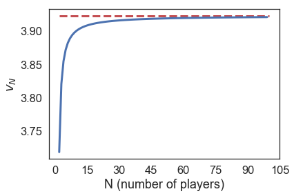
(a) $\alpha=0.2$

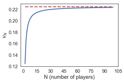
(b) $\alpha=2$

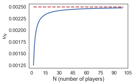
(c) $\alpha=20$

Figure 3: Convergence of $v_{N}$ with different discount factors

Remark 12.1.

Figure 3 indicates that $v_{N}$ is an increasing function of $N$ given any fixed decay parameter $\alpha$. This implies that when the number of players increases, it is more costly for players to keep track of other players before making decisions. Meanwhile, $v^{*}(x)$ being a decreasing function of $\alpha$ indicates that the bigger the $\alpha$, the less frequent players will intervene.

4.2 Approximating the $N$-player Game by the MFG

One can further show that the NE of MFG given in (3.2) is an $\epsilon$-NE for the game in (2.2).

Definition 13 ($\epsilon$-NE).

For the game (2.2) with an initial distribution $\mu_{0-}$, a control vector $\boldsymbol{\xi}=({\xi}^{1},\ldots,{\xi}^{N})$ is called its $\epsilon$-NE, if for any $i=1,\ldots,N$ and any control ${\xi}^{i^{\prime}}$ such that $\left(\boldsymbol{\xi}^{-i},{\xi}^{i^{\prime}}\right)=\left({\xi}^{1},\ldots,{\xi}^{i-1},{\xi}^{i^{\prime}},{\xi}^{i+1},\ldots,{\xi}^{N}\right)\in\mathcal{S}_{N}$,

$$\mathbb{E}\left[J^{i}_{(N)}\left(\boldsymbol{X}_{0-};\boldsymbol{\xi}\right)\right]\leq\mathbb{E}\left[J^{i}_{(N)}\left(\boldsymbol{X}_{0-};\left(\boldsymbol{\xi}^{-i},{\xi}^{i^{\prime}}\right)\right)\right]+\epsilon.$$ (4.3)

Here $X_{0-}^{i}$ $(i=1,2,\cdots,N)$ are independent samples from distribution $\mu_{0-}$, and $\mathcal{S}_{N}$ is defined in (2.9).

Theorem 14 ($\epsilon$-NE of the $N$-player game).

Let $\xi^{*}$ be the NE of MFG given in (3.2), then it is an $\epsilon$-NE of the game (2.2), with $\epsilon=O\left(\frac{1}{\sqrt{N}}\right)$.

Proof.

Given the game (2.2) with $m_{0-}=\int x\mu_{0-}(dx)\in\mathbb{R}$, assume that each player $i$ in the $N$-player game takes the control $(\xi^{i*,+}_{t},\xi^{i*,-}_{t})$ according to the NE of the MFG such that

$$\begin{aligned} \xi^{i*,+}_{t}&=&\max\left\{0,\max_{0\leq u\leq t}\left\{m_{0-}-X^{i}_{0-}-B_{u}^{i}+\xi_{u}^{i*,-}-c\right\}\right\},\\ \xi^{i*,-}_{t}&=&\max\left\{0,\max_{0\leq u\leq t}\left\{X^{i}_{0-}-m_{0-}+B_{u}^{i}+\xi_{u}^{i*,+}-c\right\}\right\}.\end{aligned}$$ (4.4)

To see that $\boldsymbol{\xi}^{*}=\left({\xi}^{1*},\ldots,{\xi}^{N*}\right)\in\mathcal{S}_{N}$, define

$$\mathcal{CW}_{mfg} = \left\{\left.\boldsymbol{x}\in\mathbb{R}^{N}\right|\ |x_{i}-m_{0-}|<c\mbox{ for }i=1,2,\cdots,N\right\},$$

$$E_{mfg,i}^{-} = \left\{\left.\boldsymbol{x}\in\mathbb{R}^{N}\right|\enspace x^{i}-m_{0-}\leq-c\right\},$$

$$E_{mfg,i}^{+} = \left\{\left.\boldsymbol{x}\in\mathbb{R}^{N}\right|\enspace x^{i}-m_{0-}\geq c\right\},$$

with the partition

$$Q_{{mfg},i} = \left\{\left.\boldsymbol{x}\in\mathbb{R}^{N}\right|\quad\left|x^{i}-m_{0-}\right|\geq\left|x^{k}-m_{0-}\right|,\mbox{ for any }k<i;\right.$$

$$\hskip 56.0pt\left.{}\left|x^{i}-m_{0-}\right|>\left|x^{k}-m_{0-}\right|,\mbox{ for any }k>i\right\}.$$

Then the control in (4.4) corresponds to the action region $\mathcal{A}_{mfg,i}=\left\{E_{mfg,i}^{-}\cup E_{mfg,i}^{+}\right\}\cap Q_{mfg,i}.$ The independence of $\{B_{t}^{1},\ldots,B_{t}^{N}\}$ and the continuity of $\{X_{t}^{1*},\ldots,X_{t}^{N*}\}_{t>0}$ imply that for any $t\geq 0$ $\mathbb{P}\left(\Pi_{i=1,\ldots,N}d\xi^{i*}_{t}=0\right)=1$.

Suppose that only one player, and without loss of generality, player one, deviates her control $\eta_{t}=(\eta_{t}^{+},\eta_{t}^{-})$ from all the other players such that $(\boldsymbol{\xi}^{-i*},{\eta})\in\mathcal{S}_{N}$. Let $\hat{X}_{t}^{1}$ be the new position of player one under control $(\eta_{t}^{+},\eta_{t}^{-})$ with initial value $X_{0-}^{1}$. Then

$$h\left(\hat{X}^{1}_{t}-\frac{1}{N}\left(\hat{X}_{t}^{1}+\sum_{j=2,\ldots,N}X_{t}^{j}\right)\right)$$

$$= h\left(\hat{X}^{1}_{t}-\frac{1}{N}\hat{X}_{t}^{1}-\frac{N-1}{N}m_{0-}\right)+h^{\prime}\left(\hat{X}^{1}_{t}-\frac{1}{N}\hat{X}_{t}^{1}-\frac{N-1}{N}m_{0-}\right)\left(\frac{\sum_{j=2,\ldots,N}X_{t}^{j}}{N}-\frac{N-1}{N}m_{0-}\right)$$

$$+\frac{h^{\prime\prime}(U_{t})}{2}\left(\frac{\sum_{j=2,\ldots,N}X_{t}^{j}}{N}-\frac{N-1}{N}m_{0-}\right)^{2},$$

where $U_{t}$ is a process between $\left(\hat{X}^{1}_{t}-\frac{1}{N}\hat{X}_{t}^{1}-\frac{N-1}{N}m_{0-}\right)$ and $\left(\hat{X}^{1}_{t}-\frac{1}{N}\left(\hat{X}_{t}^{1}+\sum_{j=2}^{N}X_{t}^{j}\right)\right)$. By Assumption A1,

$$h\left(\hat{X}^{1}_{t}-\frac{1}{N}\left(\hat{X}_{t}^{1}+\sum_{j=2,\ldots,N}X_{t}^{j}\right)\right)$$

$$\leq h\left(\hat{X}^{1}_{t}-\frac{1}{N}\hat{X}_{t}^{1}-\frac{N-1}{N}m_{0-}\right)+h^{\prime}\left(\hat{X}^{1}_{t}-\frac{1}{N}\hat{X}_{t}^{1}-\frac{N-1}{N}m_{0-}\right)\left(\frac{\sum_{j=2}^{N}X_{t}^{j}}{N}-\frac{N-1}{N}m_{0-}\right)$$

$$+\frac{K}{2}\left(\frac{\sum_{j=2}^{N}X_{t}^{j}}{N}-\frac{N-1}{N}m_{0-}\right)^{2}$$

$$\leq h\left(\hat{X}^{1}_{t}-\frac{1}{N}\hat{X}_{t}^{1}-\frac{N-1}{N}m_{0-}\right)+K\left|\hat{X}^{1}_{t}-\frac{1}{N}\hat{X}_{t}^{1}-\frac{N-1}{N}m_{0-}\right|\cdot\left|\frac{\sum_{j=2}^{N}X_{t}^{j}}{N}-\frac{N-1}{N}m_{0-}\right|$$

$$+\frac{K}{2}\left(\frac{\sum_{j=2}^{N}X_{t}^{j}}{N}-\frac{N-1}{N}m_{0-}\right)^{2}.$$

Similarly,

$$h\left(\hat{X}^{1}_{t}-\frac{1}{N}\left(\hat{X}_{t}^{1}+\sum_{j=2,\ldots,N}X_{t}^{j}\right)\right)$$

$$\geq h\left(\hat{X}^{1}_{t}-\frac{1}{N}\hat{X}_{t}^{1}-\frac{N-1}{N}m_{0-}\right)-K\left|\hat{X}^{1}_{t}-\frac{1}{N}\hat{X}_{t}^{1}-\frac{N-1}{N}m_{0-}\right|\cdot\left|\frac{\sum_{j=2}^{N}X_{t}^{j}}{N}-\frac{N-1}{N}m_{0-}\right|$$

$$-\frac{K}{2}\left(\frac{\sum_{j=2}^{N}X_{t}^{j}}{N}-\frac{N-1}{N}m_{0-}\right)^{2}.$$

Moreover, under the control (4.4), $X_{t}^{j}$ ($j=2,3,\cdots,N$) are independent and identically distributed and $|X_{t}^{j}-m_{0-}|\leq c$ a.s.. Therefore,

$$\mathbb{E}\left(\frac{\sum_{j=2}^{N}X_{t}^{j}}{N}-\frac{N-1}{N}m_{0-}\right)^{2}=\frac{\sum_{j=1}^{N}Var(X_{t}^{j})}{N^{2}}\leq\frac{c^{2}}{N}=O(\frac{1}{N}),$$

and

$$\mathbb{E}\left|\frac{\sum_{j=2}^{N}X_{t}^{j}}{N}-\frac{N-1}{N}m_{0-}\right|\leq\left(\mathbb{E}\left(\frac{\sum_{j=2}^{N}X_{t}^{j}}{N}-\frac{N-1}{N}m_{0-}\right)^{2}\right)^{1/2}=O(\frac{1}{\sqrt{N}}).$$

Therefore by the boundedness of $X_{t}^{j}$ ($j=2,3,\cdots,N$) and by the Fubini Theorem,

$$\mathbb{E}\int_{0}^{\infty}e^{-\alpha t}\left(\frac{\sum_{j=2}^{N}X_{t}^{j}}{N}-\frac{N-1}{N}m_{0-}\right)^{2}dt=\int_{0}^{\infty}e^{-\alpha t}\mathbb{E}\left(\frac{\sum_{j=2}^{N}X_{t}^{j}}{N}-\frac{N-1}{N}m_{0-}\right)^{2}dt=O\left(\frac{1}{N}\right).$$

Similarly, when $\hat{X}_{t}^{1}$ is under the threshold-type control,

$$\mathbb{E}\int_{0}^{\infty}e^{-\alpha t}\left|\hat{X}^{1}_{t}-\frac{1}{N}\hat{X}_{t}^{1}-\frac{N-1}{N}m_{0-}\right|\cdot\left|\frac{\sum_{j=2}^{N}X_{t}^{j}}{N}-\frac{N-1}{N}m_{0-}\right|dt=O(\frac{1}{\sqrt{N}}).$$ (4.5)

Now, to minimize the following payoff function

$$\mathbb{E}\int_{s}^{\infty}e^{-\alpha t}\left[h\left(\hat{X}_{t}^{1}-\frac{1}{N}\hat{X}_{t}^{1}-\frac{1}{N}\sum_{j=2}^{N}X_{t}^{j}\right)dt+d\eta_{t}^{+}+d\eta_{t}^{-}\right]$$ (4.6)

$$= \mathbb{E}\int_{s}^{\infty}e^{-\alpha t}\left[h\left(\frac{N-1}{N}\hat{X}^{1}_{t}-\frac{N-1}{N}m_{0-}\right)dt+d\eta_{t}^{+}+d\eta_{t}^{-}\right]+O\left(\frac{1}{\sqrt{N}}\right).$$

is equivalent to solving the original fuel follower problem (2.2) with a modified running cost $h(\frac{N-1}{N}(\cdot-m_{0-}))$. Since the value function for (2.2) is of a linear growth,

$$(\ref{slln}) \geq \mathbb{E}\int_{s}^{\infty}e^{-\alpha t}\left[h\left(\frac{N-1}{N}(\hat{X}^{1}_{t}-m_{0-})\right)dt+d\eta_{t}^{1*,+}+d\eta_{t}^{1*,-}\right]+O\left(\frac{1}{\sqrt{N}}\right)$$ (4.7)

$$= \mathbb{E}\left[{{v}}^{*}({X}^{1}_{0-})\right]+O\left(\frac{1}{{N}}\right)+O\left(\frac{1}{\sqrt{N}}\right)$$ (4.8)

where $v^{*}({x})$ is defined in (3.6) and the expectation in (4.8) is with respect to the initial distribution $\mu_{0-}$. The above analysis holds for any $(\eta_{t}^{+},\eta_{t}^{-})\in\mathcal{U}^{i}_{N}$ such that $(\boldsymbol{\xi}^{-i*},{\eta})\in\mathcal{S}_{N}$. Hence the conclusion. ∎

5 Discussions

5.1 Multiple Explicit NEs for $N=2$

When $N=2$, $h$ is symmetric with $h(X_{t}^{1}-m_{t}^{(2)})=h(X_{t}^{2}-m_{t}^{(2)})=h\left(\frac{X_{t}^{1}-X_{t}^{2}}{2}\right)$. This symmetry simplifies significantly the solution structure and allows for the construction of multiple NEs. Indeed, given the partition $Q_{i}$ in (2.5) for $N=2$, $Q_{1}=0$, $Q_{2}=\mathbb{R}^{2}$, one can write the NE and their corresponding values explicitly.

$$\begin{aligned} \xi^{2*}_{t}&=(\xi^{2*,+}_{t},\xi^{2*,-}_{t})\\ &=\left(\max\left\{0,\max_{0\leq u\leq t}\{-x^{2}+x^{1}-B_{u}^{2}+B_{u}^{1}+\xi_{u}^{2*,-}-c_{2}\}\right\},\right.\\ &\hskip 10.0pt\left.\max\left\{0,\max_{0\leq u\leq t}\{x^{2}-x^{1}+B_{u}^{2}-B_{u}^{1}+\xi_{u}^{2*,+}-c_{2}\}\right\}\right),\\ \xi^{1*}_{t}&=\left(\xi^{1*,+}_{t},\xi^{1*,-}_{t}\right)=(0,0),\end{aligned}$$ (5.1)

where $c_{2}>0$ is the unique positive solution of

$$\frac{1}{\sqrt{\alpha}}\tanh\left(\sqrt{\alpha}x\right)=\frac{p_{2}^{\prime}(x)-1}{p_{2}^{\prime\prime}(x)},$$ (5.2)

with

$$p_{2}(x)=\mathbb{E}\left[\int_{0}^{\infty}e^{-\alpha t}h\left(\frac{x}{2}+\frac{\sqrt{2}B_{t}}{2}\right)dt\right].$$

And the NE values are

$${v}^{2}(x^{1},x^{2})=\left\{\begin{array}[]{ll}v^{2}(x^{1},x^{1}-c_{2})-c_{2}-x^{2}+x^{1},&x^{2}-x^{1}\leq-c_{2},\\ -\frac{p_{2}^{\prime\prime}(c_{2})\cosh\left(\sqrt{\alpha}(x^{2}-x^{1})\right)}{\alpha\cosh\left(c_{2}\sqrt{\alpha}\right)}+p_{2}(x^{2}-x^{1}),&|x^{2}-x^{1}|<c_{2},\\ x^{2}-x^{1}-c_{2}+v^{2}(x^{1},x^{1}+c_{2}),&x^{2}-x^{1}\geq c_{2},\end{array}\right.$$ (5.6)

and

$$v^{1}(x^{1},x^{2})=\left\{\begin{array}[]{ll}v^{1}(x^{1},x^{1}+c_{2}),&x^{1}-x^{2}\leq-c_{2},\\ -\frac{p_{2}^{\prime\prime}(c_{2})\cosh\left(\sqrt{\alpha}(x^{1}-x^{2})\right)}{\alpha\cosh\left(c_{2}\sqrt{\alpha}\right)}+p_{2}(x^{1}-x^{2}),&|x^{2}-x^{1}|<c_{2},\\ v^{1}(x^{1},x^{1}-c_{2}),&x^{1}-x^{2}\geq c_{2}.\end{array}\right.$$ (5.10)

There is in fact more than one NE. For instance, in addition to the above constructed NE, labeled as Case 1, there are more NEs, including

1. $\mathcal{A}_{1}=\{(x^{1},x^{2})\>\lvert\>x^{1}-x^{2}>c_{2}\mbox{ or }x^{1}-x^{2}<-c_{2}\}$ and $\mathcal{A}_{2}=\emptyset$,

2. $\mathcal{A}_{1}=\{(x^{1},x^{2})\>\lvert\>x^{1}-x^{2}<-c_{2}\}$ and $\mathcal{A}_{2}=\{(x^{1},x^{2})\>\lvert\>x^{1}-x^{2}>c_{2}\}$,

3. $\mathcal{A}_{1}=\{(x^{1},x^{2})\>\lvert\>x^{1}-x^{2}>c_{2}\}$ and $\mathcal{A}_{2}=\{(x^{1},x^{2})\>\lvert\>x^{1}-x^{2}<-c_{2}\}$.

In Case 4, clearly

$$\xi_{t}^{1*} = -\max\left\{0,\max_{0\leq u\leq t}\left\{0,x^{1}-x^{2}+B_{u}^{1}-B_{u}^{2}-\xi_{u}^{2*}-c_{2}\right\}\right\},$$

$$\xi_{t}^{2*} = -\max\left\{0,\max_{0\leq u\leq t}\left\{0,x^{2}-x^{1}+B_{u}^{2}-B_{u}^{1}-\xi_{u}^{1*}-c_{2}\right\}\right\},$$

and the associated NE values are

$$v^{1}(x^{1},x^{2})=\left\{\begin{array}[]{ll}v^{1}(x^{1},x^{1}+c_{2}),&x^{1}-x^{2}\leq-c_{2},\\ -\frac{p_{2}^{{}^{\prime\prime}}(c_{2})\cosh\left(\sqrt{\alpha}(x^{1}-x^{2})\right)}{\alpha\cosh\left(c_{2}\sqrt{\alpha}\right)}+p_{2}(x^{1}-x^{2}),&|x^{1}-x^{2}|<c_{2},\\ x^{1}-x^{2}-c_{2}+v^{1}(x^{2}+c_{2},x^{2}),&x^{1}-x^{2}\geq c_{2},\end{array}\right.$$

and

$$v^{2}(x^{1},x^{2})=\left\{\begin{array}[]{ll}v^{2}(x^{2}+c_{2},x^{2}),&x^{2}-x^{1}\leq-c_{2},\\ -\frac{p_{2}^{{}^{\prime\prime}}(c_{2})\cosh\left(\sqrt{\alpha}(x^{2}-x^{1})\right)}{\alpha\cosh\left(c_{2}\sqrt{\alpha}\right)}+p_{2}(x^{2}-x^{1}),&|x^{2}-x^{1}|<c_{2},\\ x^{2}-x^{1}-c_{2}+v^{2}(x^{1},x^{1}+c_{2}),&x^{2}-x^{1}\geq c_{2}.\par\end{array}\right.$$

Figure 4 illustrates all four NEs.

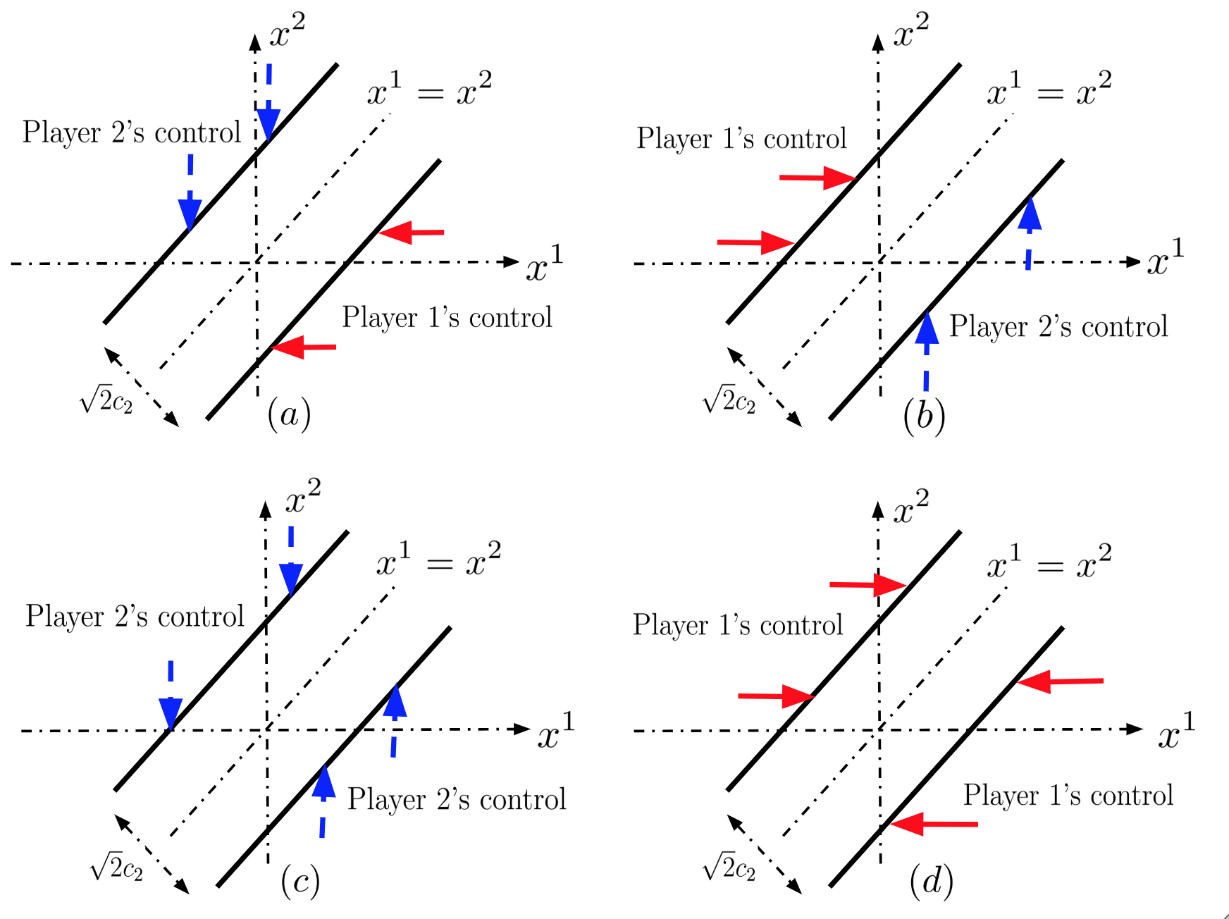
Figure 4: Four NEs when $N=2$

5.2 With Varying $\alpha$

Proposition 15.

When $h(x)=x^{2}$ and $\alpha\geq 2^{-\frac{1}{3}}\frac{N-1}{N}$, $c_{N}$ increases with respect to $\alpha$.

The proposition follows from simple calculations. Take $h(x)=x^{2}$, $\frac{p_{N}^{\prime}(x)-1}{p_{N}^{\prime\prime}(x)}=x-\frac{\alpha k_{N}^{2}}{2}$ with $k_{N}=\frac{N}{N-1}>1$. Rewrite $f_{N}$ as $f_{N}(x,\alpha)=\frac{\sqrt{k_{N}}}{\sqrt{2\alpha}}\tanh\left(\frac{\sqrt{2\alpha}}{\sqrt{k_{N}}}x\right)-x+\frac{k_{N}^{2}\alpha}{2}.$ Then $\frac{\partial f_{N}}{\partial x}=-\tanh^{2}\left(\frac{\sqrt{2\alpha}}{\sqrt{k_{N}}}x\right)$ and $\frac{\partial f_{N}}{\partial\alpha}=\frac{x}{2\alpha}\left(1-\tanh^{2}\left(\frac{\sqrt{2\alpha}}{\sqrt{k_{N}}}x\right)\right)-\frac{\sqrt{k_{N}}}{2\alpha\sqrt{2\alpha}}\tanh\left(\frac{\sqrt{2\alpha}}{\sqrt{k_{N}}}x\right)+\frac{k_{N}^{2}}{2}.$ One can verify that $\frac{\partial f_{N}}{\partial x}<0$ for any $\alpha$ and $\frac{\partial f_{N}}{\partial\alpha}>0$ when $\alpha>2^{-\frac{1}{3}}k_{N}^{-1}$. Hence $\frac{\partial c_{N}}{\partial\alpha}>0$ when $\alpha>2^{-\frac{1}{3}}k_{N}^{-1}$ follows from the chain rule and from $f(c_{N}(\alpha),\alpha)=0$ for any $N$.

Figure 5, illustrates the convergence of $c_{N}$ with different discount factor $\alpha$. The value of $c$ is shown in the red dash line.

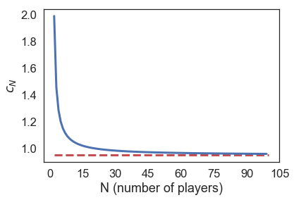
(a) $\alpha=0.2$

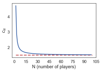
(b) $\alpha=2$

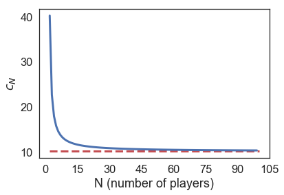
(c) $\alpha=20$

Figure 5: Convergence of $c_{N}$ with different discount factors

Remark 15.1.

Figure 5 indicates that $c_{N}$ is a decreasing function of $N$ for any given discount factor $\alpha$. This implies that players will intervene more frequently with more players in the game. Meanwhile, $c$ being a decreasing function of $\alpha$ indicates that the bigger the $\alpha$, the less frequent players will intervene. These are consistent with Figure 3.

It is worth noting that the analysis for $\alpha_{1}=\cdots=\alpha_{N}=\alpha$ can be easily extended to the cases when $\alpha_{i}$’s are different. The exact forms of the NEs, however, may be more complicated, as illustrated in the case of $N=2$ below.

When $N=2$, denote $\alpha_{i}$ as the discount parameter for player $i$ ($i=1,2$). Denote $c_{2}^{(i)}>0$ as the unique solution of

$$\frac{1}{\sqrt{\alpha_{i}}}\tanh\left(\sqrt{\alpha_{i}}x\right)=\frac{p_{2}^{\prime}(x,\alpha_{i})-1}{p_{2}^{\prime\prime}(x,\alpha_{i})},$$ (5.13)

with

$$p_{2}(x,\alpha_{i})=\mathbb{E}\left[\int_{0}^{\infty}e^{-\alpha_{i}t}h\left(\frac{x}{2}+\frac{\sqrt{2}B_{t}}{2}\right)dt\right].$$

Corollary 15.1 ($N=2$ with $\alpha_{1}\neq\alpha_{2}$).

Assume A1 for game (2.2). If $\alpha_{2}>\alpha_{1}>2^{-\frac{4}{3}}$, then $c_{2}^{(2)}>c_{2}^{(1)}$. The following controls

$$\xi_{t}^{2*,+} = \textbf{1}_{\left\{x^{2}-x^{1}<-c_{2}^{(2)}\right\}}\left(-c_{2}^{(2)}-x^{2}+x^{1}\right),$$

$$\xi_{t}^{2*,-} = \textbf{1}_{\left\{x^{2}-x^{1}>c_{2}^{(2)}\right\}}\left(c_{2}^{(2)}-x^{2}+x^{1}\right),$$

and

$$\xi_{t}^{1*,+} = \max\left\{0,\max_{0\leq u\leq t}\{x^{2}+B_{u}^{2}+\xi_{0}^{2*,+}-\xi_{0}^{2*,-}-x^{1}-{B}^{1}_{u}+\xi_{u}^{1*,-}-c_{2}^{(1)}\}\right\},$$

$$\xi_{t}^{1*,-} = \max\left\{0,\max_{0\leq u\leq t}\{-x^{2}-B_{u}^{2}-\xi_{0}^{2*,+}+\xi_{0}^{2*,-}+x^{1}+{B}^{1}_{u}+\xi_{u}^{1*,+}-c_{2}^{(1)}\}\right\}.$$

give a Markovian NE. The corresponding NE values are

$$v^{1}(x^{1},x^{2})=\left\{\begin{array}[]{ll}v^{1}({x^{1},x^{1}+c_{2}^{(2)}})&x^{1}-x^{2}\leq-c_{2}^{(2)},\\ v^{1}(x^{2}-c_{2}^{(1)},x^{2})+x^{2}-x^{1}-c_{2}^{(1)},&-c_{2}^{(2)}\leq x^{1}-x^{2}\leq-c_{2}^{(1)},\\ -\frac{p_{2}^{{}^{\prime\prime}}(c^{(1)}_{2})\cosh\left(\sqrt{\alpha}(x^{1}-x^{2})\right)}{\alpha\cosh\left(c^{(1)}_{2}\sqrt{\alpha}\right)}+p_{2}(x^{1}-x^{2}),&|x^{1}-x^{2}|\leq c^{(1)}_{2},\\ x^{1}-x^{2}-c^{(1)}_{2}+v^{1}(x^{2}+c^{(1)}_{2},x^{2}),&c^{(1)}_{2}\leq x^{1}-x^{2}\leq c^{(2)}_{2},\\ v^{1}({x^{1},x^{1}-c_{2}^{(2)}})&x^{1}-x^{2}\geq c^{(2)}_{2},\end{array}\right.$$ (5.19)

and

$$v^{2}(x^{1},x^{2})=\left\{\begin{array}[]{ll}v^{2}(x^{1},x^{1}-c^{(2)}_{2}){+x^{1}-x^{2}-c_{2}^{(2)}},&x^{2}-x^{1}\leq-c^{(2)}_{2},\\ {v^{2}(x^{2}+c_{2}^{(1)},x^{2})}&-c^{(2)}_{2}\leq x^{2}-x^{1}\leq-c^{(1)}_{2},\\ -\frac{p_{2}^{{}^{\prime\prime}}({c^{(1)}_{2}})\cosh\left(\sqrt{\alpha}(x^{2}-x^{1})\right)}{\alpha\cosh\left({c^{(1)}_{2}}\sqrt{\alpha}\right)}+p_{2}(x^{2}-x^{1}),&|x^{2}-x^{1}|\leq{c^{(1)}_{2}},\\ {v^{2}(x^{2}-c_{2}^{(1)},x^{2})}&c^{(1)}_{2}\leq x^{2}-x^{1}\leq c^{(2)}_{2},\\ x^{2}-x^{1}-c^{(2)}_{2}+v^{2}(x^{1},x^{1}+c_{2}^{(2)}),&x^{2}-x^{1}\geq c^{(2)}_{2}.\par\end{array}\right.$$ (5.25)

Figure 6 shows the NE defined in Corollary 15.1.

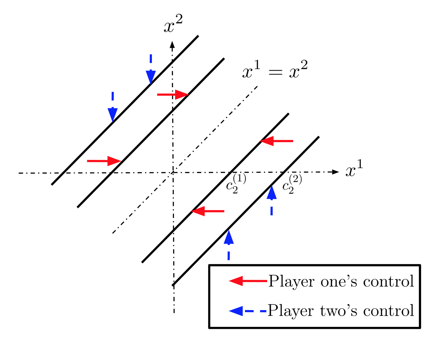
Figure 6: N=2 with different $\alpha$ values

Acknowledgments.

The authors are in debt to the referee and the AE for their invaluable suggestions and extremely insightful remarks.

Appendix A: the Skorokhod Problem (SP)

First, some notation for a general polyhedron G.

Take a fixed integer $l$ ($l\geq 1$), let $\boldsymbol{J}=\{1,2,\cdots,l\}$. Given an $l-$dimensional vector $\boldsymbol{b}=(b_{1},\cdots,b_{l})$ and $N$-dimensional unit vectors $\{\boldsymbol{n}_{j},j\in\boldsymbol{J}\}$, a polyhedron $G$ is defined by

$$G=\{\boldsymbol{x}\in\mathbb{R}^{N}\ |\ \boldsymbol{n}_{j}\cdot\boldsymbol{x}>b_{j}\mbox{ for any }j\in\boldsymbol{J}\}.$$

Assume the faces $F_{j}=\{\boldsymbol{x}\in\bar{G}\ |\ \boldsymbol{n}_{j}\cdot\boldsymbol{x}=b_{j}\}$ ($j\in\boldsymbol{J}$) are of dimension ${N}-1$.

Next, take another set of $N-$dimensional vectors $\{\boldsymbol{d}_{j},j\in\boldsymbol{J}\}$, we can define the SP problem on a polyhedron with oblique reflections $(\boldsymbol{d_{1}},\cdots,\boldsymbol{d_{l}})$, in both the strong sense and the weak sense.

Definition 16 (Strong solution to SP).

Given a polyhedron $G$, a vector field $(\boldsymbol{d_{1}},\cdots,\boldsymbol{d_{l}})$, and $\boldsymbol{x}\in\overline{G}$. Given an $N$-dimensional Brownian motion $\{\boldsymbol{B}_{t}\}_{t\geq 0}$ on the probability space $(\Omega,\mathcal{F},\mathbb{P}_{\boldsymbol{x}})$, a strong solution to the SP with the data $\left(\boldsymbol{x},G,(\boldsymbol{d_{1}},\cdots,\boldsymbol{d_{l}}),\{B_{t}\}_{t\geq 0}\right)$ is an $\mathcal{F}_{t}^{B}$-adapted process $\boldsymbol{X}_{t}$ such that

1. $\boldsymbol{X}_{t}=\boldsymbol{x}+\boldsymbol{B}_{t}+\boldsymbol{\eta}_{t}D$, with $D=\begin{bmatrix}\boldsymbol{d}^{1}\\ \cdots\\ \boldsymbol{d}^{l}\end{bmatrix}\in\mathbb{R}^{l\times N}$,

2. $\boldsymbol{X}_{t}$ has a continuous path in $\overline{G}$,

3. $\boldsymbol{X}_{t}\in\overline{G},\quad\mbox{ for any }t\geq 0\mbox{ a.s.}$,

4. $\eta^{j}_{0}=0$, $\eta^{j}_{t}$ is continuous and nondecreasing, $\eta^{j}_{t}$ increases only when $\boldsymbol{X}_{t}$ is on the face $F_{j}$. That is,

   $${\eta}^{j}_{t}=\int_{0}^{t}\textbf{1}_{\left\{\boldsymbol{X}_{s}\in\partial F_{j}\right\}}d{\eta}^{j}_{s},$$

5. the reflection direction $\gamma(\boldsymbol{x}):=\boldsymbol{d}_{j},\mbox{ if }\boldsymbol{x}\in F_{j}\mbox{ for }j\in\boldsymbol{J}.$

Definition 17 (Weak solution to SP).

Given a polyhedron $G$, a vector field $(\boldsymbol{d_{1}},\cdots,\boldsymbol{d_{l}})$, and $\boldsymbol{x}\in\bar{G}$. A weak solution to the SP with the data $\left(\boldsymbol{x},G,(\boldsymbol{d_{1}},\cdots,\boldsymbol{d_{l}})\right)$ is an adapted $N$-dimensional process $\boldsymbol{X}_{t}$ defined on some probability space $(\Omega,\mathcal{F},\mathbb{P}_{\boldsymbol{x}})$ such that

1. $\boldsymbol{X}_{t}=\boldsymbol{W}_{t}+\boldsymbol{\eta}_{t}D$, with $D=\begin{bmatrix}\boldsymbol{d}^{1}\\ \cdots\\ \boldsymbol{d}^{l}\end{bmatrix}\in\mathbb{R}^{l\times N}$ and $\boldsymbol{W}$ an $N$-dimensional Brownian motion under $\mathbb{P}_{\boldsymbol{x}}$, with $\boldsymbol{X}_{0}=\boldsymbol{x}$, $\mathbb{P}_{\boldsymbol{x}}$-a.s.,

2. $\boldsymbol{X}_{t}$ has a continuous path in $\overline{G}$, $\mathbb{P}_{\boldsymbol{x}}$-a.s.,

3. $\eta^{j}_{0}=0$, $\eta^{j}_{t}$ is continuous and nondecreasing, $\eta^{j}(t)$ can increase only when $\boldsymbol{X}_{t}$ is on the face $F_{j}$. That is,

   $${\eta}^{j}_{t}=\int_{0}^{t}\textbf{1}_{\left\{\boldsymbol{X}_{s}\in\partial F_{j}\right\}}d{\eta}^{j}_{s},$$

4. the reflection direction $\gamma(\boldsymbol{x}):=\boldsymbol{d}_{j},\mbox{ if }\boldsymbol{x}\in F_{j}\mbox{ for }j\in\boldsymbol{J}.$

Now the proof of Theorem 4 follows from the following two lemmas.

Lemma 18 (Existence of the weak solution to SP).

Fix $\boldsymbol{x}\in\overline{\mathcal{CW}}$. There exists a weak solution to the SP with the data $(\mathcal{CW},(\boldsymbol{d}_{1},\cdots,\boldsymbol{d}_{2N}),\boldsymbol{x})$ with $\boldsymbol{d}_{j}$ $(j=1,2,\cdots,2N)$ defined in (2.25) and $\mathcal{CW}$ defined in (2.6). It is a semimartingale reflected Brownian motion (SRBM) starting from $\boldsymbol{x}$.

In fact, this weak solution is unique in a weak sense, see [14].

Proof of Lemma 18.

Following the notation in [14], define the maximal set to characterize the points on $\partial\mathcal{CW}$ as follows. Take $\textbf{J}=\{1,2,\cdots,2N\}$ the index set of the $2N$ faces of $\mathcal{CW}$. For each $\varnothing\neq\boldsymbol{K}\subset\textbf{J}$, define $F_{\textbf{K}}=\cap_{j\in\textbf{K}}F_{j}$. Let $F_{\varnothing}=\mathcal{CW}$. A set $\boldsymbol{K}\subset\boldsymbol{J}$ is maximal if $\textbf{K}\neq\varnothing$, $F_{\textbf{K}}\neq\varnothing$, and $F_{\textbf{K}}\neq F_{\tilde{\textbf{K}}}$ for any $\tilde{\textbf{K}}\supset{\textbf{K}}$ such that $\tilde{\textbf{K}}\neq{\textbf{K}}$. Now, it suffices to show that for each maximal $\boldsymbol{K}\subset\boldsymbol{J}$,

• there is a positive linear combination $\boldsymbol{d}=\sum_{j\in\boldsymbol{K}}\ a_{j}\boldsymbol{d}_{j}$ ($a_{j}>0,\ \forall j\in\boldsymbol{K}$) of the $\{\boldsymbol{d}_{j},\ j\in\boldsymbol{K}\}$ such that $\boldsymbol{n}_{j}\cdot\boldsymbol{d}>0$ for any $j\in\boldsymbol{K}$;

• there is a positive linear combination $\boldsymbol{n}=\sum_{j\in\boldsymbol{K}}c_{j}\boldsymbol{n}_{j}$ ($c_{j}>0,\ \forall j\in\boldsymbol{K}$) of the $\{\boldsymbol{n}_{j},\ j\in\boldsymbol{K}\}$ such that $\boldsymbol{d}_{j}\cdot\boldsymbol{n}>0$ for any $j\in\boldsymbol{K}$.

Let us first show that for any maximal $\boldsymbol{K}$, $|\boldsymbol{K}|\leq N-1$. To see this claim, denote

$$N_{\mbox{mat}}:=\begin{bmatrix}\boldsymbol{n}_{1}\\ \boldsymbol{n}_{2}\\ \vdots\\ \boldsymbol{n}_{2N}\end{bmatrix}=\frac{\sqrt{N-1}}{\sqrt{N}}\begin{bmatrix}1&-\frac{1}{N-1}&-\frac{1}{N-1}&\dots&-\frac{1}{N-1}\\ -\frac{1}{N-1}&1&-\frac{1}{N-1}&\dots&-\frac{1}{N-1}\\ \vdots&\vdots&\vdots&\ddots&\vdots\\ -\frac{1}{N-1}&-\frac{1}{N-1}&-\frac{1}{N-1}&\dots&1\\ -1&\frac{1}{N-1}&\frac{1}{N-1}&\dots&\frac{1}{N-1}\\ \frac{1}{N-1}&-1&\frac{1}{N-1}&\dots&\frac{1}{N-1}\\ \vdots&\vdots&\vdots&\ddots&\vdots\\ \frac{1}{N-1}&\frac{1}{N-1}&\frac{1}{N-1}&\dots&-1\end{bmatrix}\in\mathbb{R}^{2N\times N}.$$

It follows from some calculations that $\det(N_{\mbox{mat}})=N-1$, implying that for any $\boldsymbol{K}\subset\boldsymbol{J}$ with $|\boldsymbol{K}|=N$, $\cap F_{j\in\boldsymbol{K}}=\varnothing$. Moreover, for any maximal K, $|\boldsymbol{K}|\leq N-1$. Now checking the conditions (S.a) and (S.b) for any maximal $\boldsymbol{K}$ reduces to checking these conditions for the maximal $\boldsymbol{K}$ with $|\boldsymbol{K}|=N-1$.

Note that for any $i=1,\cdots,N$, $F_{i}$ and $F_{N+i}$ are parallel faces such that $F_{i}\cap F_{N+i}=\varnothing$, there is no maximal $\boldsymbol{K}$ for which both $i\in\boldsymbol{K}$ and $N+i\in\boldsymbol{K}$. Thus, take any $\boldsymbol{K}=\{i_{1},\cdots,i_{N-1}\}$, where $i_{k}\in\{k,N+k\}$ for $k=1,2,\cdots,N-1$. Denote $m$ as the number of indexes in $\boldsymbol{K}$ which is strictly smaller than $N$, then $N-1-m$ is the number of indexes in $\boldsymbol{K}$ that are greater than $N$.

To check (S.a), define $\boldsymbol{n}=\sum_{k=1}^{N-1}\boldsymbol{n}_{i_{k}}$, then for any $k\in\{1,2,\cdots,N-1\}$,

$$\boldsymbol{n}\cdot\boldsymbol{d}_{i_{k}}=\frac{\sqrt{N-1}}{\sqrt{N}}\left[1+\frac{1}{N-1}\left[\boldsymbol{1}_{(i_{k}\leq N)}(N-2m)+\boldsymbol{1}_{(i_{k}>N)}(-N{+2m}+2)\right]\right]>0.$$

To check (S.b), define $d=\sum_{k=1}^{N-1}d_{i_{k}}$, then for any $k\in\{1,2,\cdots,N-1\}$,

$$\boldsymbol{d}\cdot\boldsymbol{n}_{i_{k}}=\frac{\sqrt{N-1}}{\sqrt{N}}\left[1+\frac{1}{N-1}\left[\boldsymbol{1}_{(i_{k}\leq N)}(N-2m)+\boldsymbol{1}_{(i_{k}>N)}(-N{+2m}+2)\right]\right]>0.$$

∎

Next, the uniqueness of solution in the strong sense is established by the localization technique. That is, construct a sequence of bounded region $\mathcal{W}_{k}$ ($k\in\mathbb{N}^{+}$) such that

$$\mathcal{W}_{1}\subset\mathcal{W}_{2}\subset\cdots\subset\mathcal{CW},$$

where $\mathcal{W}_{k}$ satisfies the condition in [16]. Then define a sequence of stopping times associated with $\mathcal{W}_{k}$ ($k\in\mathbb{N}^{+}$) and extend the strong uniqueness result on bounded regions in [16].

Lemma 19 (Uniqueness of the strong solution to SP).

Given a probability space $(\Omega,\mathcal{F},\mathbb{P})$, suppose there are two strong solutions $\boldsymbol{X}_{t}^{*}$ and $\boldsymbol{X}_{t}^{*\prime}$ to the SP with the data $\left(\boldsymbol{x},\mathcal{CW},(\boldsymbol{d}_{1},\cdots,\boldsymbol{d}_{2N}),\{\boldsymbol{B}_{t}\}_{t\geq 0}\right)$ with $\boldsymbol{d}_{i}$ $(i=1\cdots,2N)$ defined in (2.25). Then

$$\mathbb{P}_{\boldsymbol{x}}\left(\boldsymbol{X}_{t}^{*}=\boldsymbol{X}_{t}^{*\prime};\quad 0\leq t<\infty\right)=1.$$

Proof of Lemma 19..

First, the uniqueness on a bounded region. To this end, define the bounded region $\mathcal{W}_{k}=\mathcal{CW}\cap\left\{\boldsymbol{x}\ \left|\ \left|\sum_{i=1}^{N}x_{i}\right|<k\right.\right\}$ for $k\in\mathbb{N}_{+}$. Clearly, $\mathcal{W}_{k}\subseteq\mathcal{W}_{k+1}\subseteq\mathcal{CW}$ and $\mathcal{CW}=\cup_{k}\mathcal{W}_{k}$. Define the boundaries of $\mathcal{W}_{k}$ as

$$\partial\mathcal{W}_{k}=\cup_{i=1}^{2N}F_{i}^{(k)}\cup F_{2N+1}^{(k)}\cup F_{2N+2}^{(k)},$$

where $F_{i}^{(k)}=F_{i}\cap\overline{\mathcal{W}}_{k}$ for $i=1,\ldots,2N$, $F_{2N+1}^{(k)}=\overline{\mathcal{W}}_{k}\cap\{\boldsymbol{x}\>\lvert\>\sum_{i=1}^{N}x_{i}=k\}$, and $F_{2N+2}^{(k)}=\overline{\mathcal{W}}_{k}\cap\{\boldsymbol{x}\>\lvert\>\sum_{i=1}^{N}x_{i}=-k\}$. Define the reflection direction $\gamma^{(l)}(\cdot)$ on $\partial\mathcal{W}_{k}$ as

$$\gamma^{(k)}(\boldsymbol{x})=\left\{\begin{array}[]{ll}&\boldsymbol{d}_{2N+1}=\boldsymbol{n}_{2N+1}=\frac{1}{\sqrt{N}}(-1,-1,\ldots,-1),\,\,\boldsymbol{x}\in F_{2N+1}^{(k)},\\ &\boldsymbol{d}_{2N+2}=\boldsymbol{n}_{2N+2}=\frac{1}{\sqrt{N}}(1,1,\ldots,1),\,\,\boldsymbol{x}\in F_{2N+2}^{(k)},\\ &\boldsymbol{d}_{i},\,\,\boldsymbol{x}\in F_{i}^{(k)},\mbox{ for }i=1,2,\cdots,2N.\end{array}\right.$$ (5.29)

For $\boldsymbol{x}\in\partial\mathcal{W}_{k}$, define $I_{k}(\boldsymbol{x}):=\left\{i:\boldsymbol{x}\in F_{i}^{(k)}\right\}$ as the index set of $\boldsymbol{x}$. Following [16], we will show that, for each $\boldsymbol{x}\in\partial\mathcal{W}_{k}$, there exists $b_{i}\geq 0$, $i\in I_{k}(\boldsymbol{x})$, such that

$$b_{i}\boldsymbol{d}_{i}\cdot\boldsymbol{n}_{i}>\sum_{j\in I_{k}(\boldsymbol{x})\setminus\{i\}}b_{j}|\boldsymbol{d}_{j}\cdot\boldsymbol{n}_{i}|.\qquad\qquad\mbox{{(S.c)}}$$

Define $b_{i}=1$ for any $i=1,2,\cdots,2N+2$. It is sufficient to verify (S.c) for $\boldsymbol{x}\in\partial\mathcal{W}_{k}$ such that $|I_{k}(\boldsymbol{x})|=N$. In this case, either $2N+1\in I_{k}(\boldsymbol{x})$ or $2N+2\in I_{k}(\boldsymbol{x})$. Take any $i_{0}\in I_{k}(\boldsymbol{x})\setminus\{2N+1,2N+2\}$,

$$|\boldsymbol{n}_{i_{0}}\cdot\boldsymbol{d}_{i_{0}}| = \frac{\sqrt{N-1}}{\sqrt{N}},$$

$$|\boldsymbol{n}_{i_{0}}\cdot\boldsymbol{d}_{j}| = \frac{\sqrt{N-1}}{\sqrt{N}}\frac{1}{N-1},\quad\mbox{ for }j\in I_{k}(\boldsymbol{x})\setminus\{2N+1,2N+2,i_{0}\},$$

$$|\boldsymbol{n}_{i_{0}}\cdot\boldsymbol{d}_{j}| = 0,\quad\mbox{ for }j\in\{2N+1,2N+2\}.$$

Hence (S.c) holds with $\boldsymbol{d}_{i_{0}}\cdot\boldsymbol{n}_{i_{0}}=\frac{\sqrt{N-1}}{\sqrt{N}}$ and $\sum_{j\in I_{k}(\boldsymbol{x})\setminus\{i_{0}\}}|\boldsymbol{d}_{j}\cdot\boldsymbol{n}_{i_{0}}|=\frac{\sqrt{N-1}}{\sqrt{N}}\frac{N-2}{N-1}$. By [16], there exists a unique strong solution $(\boldsymbol{X}^{k}_{t},\boldsymbol{\eta}^{k})_{t\geq 0}$ to the SP with the data $\left(\boldsymbol{x},\mathcal{W}_{k},(\boldsymbol{d}_{1},\cdots,\boldsymbol{d}_{2N+2}),\{\boldsymbol{B}_{t}\}_{t\geq 0}\right)$ such that $\boldsymbol{x}\in\overline{\mathcal{W}}_{k}$.

Now, let $(\boldsymbol{X}_{t}^{k\prime},\boldsymbol{\eta}^{k\prime})$ be the strong solution to the SP with the data $\left(\boldsymbol{x}^{\prime},\mathcal{W}_{k},(\boldsymbol{d}_{1},\cdots,\boldsymbol{d}_{2N+2}),\{\boldsymbol{B}^{\prime}_{t}\}_{t\geq 0}\right)$. Then by [16], there exists a constant $C_{k}<\infty$ such that for any $0\leq t\leq T$,

$$\mathbb{E}\left(\sup_{0\leq s\leq t}\|\boldsymbol{X}_{s}^{k}-\boldsymbol{X}_{s}^{k\prime}|^{2}\right)\leq C_{k}\left\{\|\boldsymbol{x}-\boldsymbol{x}^{\prime}\|^{2}+\int_{0}^{t}\mathbb{E}\left(\sup_{0\leq u\leq s}\|\boldsymbol{B}_{s}-\boldsymbol{B}_{s}^{\prime}\|^{2}\right)ds\right\}.$$ (5.30)

To finish the proof, now suppose that there are two strong solutions $(\boldsymbol{X}_{t}^{*},\boldsymbol{\eta}^{*})_{t\geq 0}$ and $(\boldsymbol{X}_{t}^{*\prime},\boldsymbol{\eta}^{*\prime})_{t\geq 0}$ to the SP with the data $\left(\boldsymbol{x},\mathcal{CW},(\boldsymbol{d}_{1},\cdots,\boldsymbol{d}_{2N}),\{\boldsymbol{B}_{t}\}_{t\geq 0}\right)$, with $\boldsymbol{d}_{i}$ $(i=1,2,\cdots,2N)$ defined in (2.25) and $\boldsymbol{X}_{0}^{*}=\boldsymbol{X}_{0}^{*\prime}=\boldsymbol{x}\in\overline{\mathcal{CW}}$. Suppose there exists $M:=M(\boldsymbol{x})$ such that $\boldsymbol{x}\in\overline{\mathcal{W}}_{k}$ for $k\geq M$. Define $\tau_{k}=\inf\{t:\boldsymbol{X}_{t}^{*}\in F^{(k)}_{2N+1}\cup F^{(k)}_{2N+2}\}$ and $\tau_{k}^{\prime}=\inf\{t:\boldsymbol{X}_{t}^{*\prime}\in F^{(k)}_{2N+1}\cup F^{(k)}_{2N+2}\}$. Then the uniqueness of the strong solution to SP with the data $(\boldsymbol{x},\mathcal{W}_{k},\gamma^{(k)},\{\boldsymbol{B}_{t}\}_{t\geq 0})$ implies that for $k\geq M$,

$$\mathbb{P}_{\boldsymbol{x}}\left(\boldsymbol{X}_{t}^{*}=\boldsymbol{X}_{t}^{*\prime},\ t\leq\tau_{k}\right)=1,$$ (5.31)

$$\mathbb{P}_{\boldsymbol{x}}\left(\tau_{k}=\tau_{k}^{\prime}\right)=1.$$

By the continuity of the probability measure,

$$\mathbb{P}_{\boldsymbol{x}}\left(\boldsymbol{X}_{t}^{*}=\boldsymbol{X}_{t}^{*}{{}^{\prime}},\ t\leq\tau_{k},k\rightarrow\infty\right)=\lim_{k\rightarrow\infty}\mathbb{P}_{\boldsymbol{x}}\left(\boldsymbol{X}_{t}^{*}=\boldsymbol{X}_{t}^{*\prime},\ t\leq\tau_{k}\right)=1.$$ (5.32)

Now it remains to show $\lim_{k\rightarrow\infty}\tau_{k}=\infty$ a.s.. Suppose otherwise, then there exists $\tau^{*}=\tau^{*}(\omega)<\infty$ such that $\lim_{k\rightarrow\infty}\tau_{k}=\tau^{*}$ pathwise. Therefore,

$$\mathbb{P}_{\boldsymbol{x}}\left(\ \left|\sum_{i=1}^{N}{X}_{\tau^{*}}^{i*}\right|=\infty\ \right)=\mathbb{P}_{\boldsymbol{x}}\left(\ \left|\sum_{i=1}^{N}{x}^{i}+{B}_{\tau^{*}}^{i}+\eta_{\tau^{*}}^{i*}-\eta_{\tau^{*}}^{N+i*}\right|=\infty\ \right)=1,$$

which implies, from the bounded variation property of $\{\boldsymbol{\eta}^{*}\}_{t\geq 0}$, $\mathbb{P}_{\boldsymbol{x}}\left(\left|\sum_{i=1}^{N}B_{\tau^{*}}^{i}\right|=\infty\right)=1.$ This contradicts with the property of Brownian motion, thus $\lim_{k\rightarrow\infty}\tau_{k}=\infty$ a.s.. ∎

Appendix B: Well-posedness of Algorithm 1

If $\boldsymbol{x}=(x^{1},\cdots,x^{N})\notin\overline{\mathcal{CW}}$, then there exists an $i$ such that $\boldsymbol{x}\in\mathcal{A}_{i}$. For any $k>1$, denote the point after the $k$-th jump as $\boldsymbol{x}_{k}=(x^{1}_{k},\ldots,x^{N}_{k})$. In step $k+1$, if $\boldsymbol{x}_{k}\in\mathcal{A}_{i}$, player $i$ will apply a minimal push to reach the boundary $\partial E_{i}^{-}\cup\partial E_{i}^{+}$.

If the jumps do not stop in finite steps, an argument by contradiction will show that they converge to $\hat{\boldsymbol{x}}\in\partial{\mathcal{CW}}$. Let us first show that $\{\boldsymbol{x}_{k}\}_{k\geq 1}$ converges. At each step $k\geq 1$, denote $x^{(1)}_{k}\leq\cdots\leq x^{(N)}_{k}$ as the ordered points of $x^{1}_{k},\ldots,x^{N}_{k}$. At each step $k$, only the player with position ${x}^{(1)}_{k}$ or ${x}^{(N)}_{k}$ will jump. Therefore $\{x^{(1)}_{k}\}_{k\geq 1}$ is a non-decreasing sequence with an upper bound $\max_{i\leq N}x^{i}$. Hence the limit exists, denoted as $x^{(1)}_{*}$. Similarly, the bounded non-increasing sequence $x^{(N)}_{k}$ has a limit, denoted as $x_{*}^{(N)}$. Then by the sandwich argument, $\{\boldsymbol{x}_{k}\}_{k\geq 1}$ converges.

Next, denote the distance $d^{i}_{k}=|x^{i}_{k}-\frac{\sum_{i\neq j}{x^{j}_{k}}}{N-1}|$. By definition of $\mathcal{A}_{i}$, the player with the biggest $d^{i}_{k}$ will jump in step $k+1$. Suppose $\hat{\boldsymbol{x}}=\lim_{k\rightarrow\infty}\boldsymbol{x}_{k}\notin\partial{\mathcal{CW}}$, then there exists an $m\in\{1,\ldots,N\}$ such that $\hat{\boldsymbol{x}}\in\mathcal{A}_{m}$. Denote the distance $\Delta=|\hat{{x}}^{m}-\frac{\sum_{j\neq m}\hat{{x}}^{j}}{N-1}|-c_{N}=\max_{i=1,2,\cdots,N}\{|\hat{{x}}^{i}-\frac{\sum_{j\neq i}\hat{{x}}^{j}}{N-1}|\}-c_{N}>0$. Given $\epsilon>0$ so that $\epsilon<\frac{\Delta}{8N}$ and $\overline{\mathcal{CW}}\cap{B}_{\epsilon}(\hat{\boldsymbol{x}})=\emptyset$, there exists a sufficiently large $K>0$ such that for any $k^{\prime}>K$, $\boldsymbol{x}_{k{{}^{\prime}}}\in B_{\epsilon}(\hat{\boldsymbol{x}}).$ That is, $\sum_{i=1}^{N}|{x}^{i}_{k{{}^{\prime}}}-\hat{{x}}^{i}|^{2}\leq\epsilon^{2}$. By the triangle inequality,

$$\left|x^{m}_{k^{\prime}}-\frac{\sum_{j\neq m}x_{k^{\prime}}^{j}}{N-1}\right|-c_{N} \geq \left|\hat{{x}}^{m}-\frac{\sum_{j\neq m}\hat{{x}}^{j}}{N-1}\right|-c_{N}-\left|\left(x^{m}_{k^{\prime}}-\frac{\sum_{j\neq m}x_{k^{\prime}}^{j}}{N-1}\right)-\left(\hat{{x}}^{m}-\frac{\sum_{j\neq m}\hat{{x}}^{j}}{N-1}\right)\right|$$

$$\geq \left|\hat{{x}}^{m}-\frac{\sum_{j\neq m}\hat{{x}}^{j}}{N-1}\right|-c_{N}-\left|x^{m}_{k^{\prime}}-\hat{{x}}^{m}\right|-\frac{1}{N-1}\sum_{j\neq m}\left|x_{k^{\prime}}^{j}-\hat{{x}}^{j}\right|$$

$$\geq \Delta-2\epsilon\geq\frac{4N-1}{4N}\Delta>2\epsilon.$$

Thus in step $k^{\prime}+1$, the player should jump at a minimum distance of $\frac{4N-1}{4N}\Delta$, which is strictly greater than $2\epsilon$ when $N>1$. Therefore $\boldsymbol{x}_{k^{\prime}+1}\notin B_{\epsilon}(\hat{\boldsymbol{x}})$, which is a contradiction. Hence $\hat{\boldsymbol{x}}=\lim_{k\rightarrow\infty}\boldsymbol{x}_{k}\in\partial\overline{\mathcal{CW}}.$

To see that the total distance of sequential jumps is bounded, rewrite $d^{i}_{k}$ in the form of $d^{i}_{k}=\frac{N-1}{N}\left|x^{i}_{k}-\bar{x}_{k}\right|$, where $\bar{x}_{k}=\frac{\sum_{j=1}^{N}x^{j}_{k}}{N}$. Clearly, in step $k+1$, either the player with value $x^{(1)}_{k}$ or the player with value $x^{(N)}_{k}$ will jump. By the monotonicity property of $\{x^{(N)}_{k}\}_{k}$ and $\{x^{(1)}_{k}\}_{k}$, the total distance of jumps is bounded pointwise.

Appendix C: Proof of Proposition 11

Proof.

First, denote for $N\geq 2$,

$$f_{N}(x)=\frac{1}{\sqrt{\frac{2(N-1)\alpha}{N}}}\tanh\left(x\sqrt{\frac{2(N-1)\alpha}{N}}\right)-\frac{p^{\prime}_{N}(x)-1}{p^{\prime\prime}_{N}(x)},$$

and

$$f_{1}(x)=\frac{1}{\sqrt{{2\alpha}}}\tanh\left(x\sqrt{2\alpha}\right)-\frac{p^{\prime}_{1}(x)-1}{p^{\prime\prime}_{1}(x)}.$$

Then there exists a unique $c>0$ such that $f_{1}(c)=0$ and there exists a unique $c_{N}>0$ such that $f_{N}(c_{N})=0$ for $N\geq 2$. Denote $m_{1}(x)=\frac{p^{\prime}_{1}(x)-1}{p^{\prime\prime}_{1}(x)}$ and $m_{N}(x)=\frac{p^{\prime}_{N}(x)-1}{p^{\prime\prime}_{N}(x)}$. There exists $\tilde{c}_{N}>0$ such that $m^{\prime}_{N}(x)\geq 1$ on $(\tilde{c}_{N},\infty)$ with $0<\tilde{c}_{N}<c_{N}<\infty$ for $N\geq 2$. And there exists $\tilde{c}>0$ such that $m^{\prime}_{1}(x)\geq 1$ on $(\tilde{c},\infty)$ with $0<\tilde{c}<c<\infty$. Now $0<\tanh^{\prime}(x)=1-\tanh^{2}(x)<1$ for any $x\in(0,\infty)$, therefore $f^{\prime}_{N}(x)<0$ on $(c_{N},\infty)$ for $N\geq 2$ and $f^{\prime}_{1}(x)<0$ on $(c,\infty)$. Since $f_{N}$ converges to $f_{1}$ pointwise, for any $\epsilon>0$, there exists an $N_{\epsilon}$ such that for any $n\geq N_{\epsilon}$, $|f_{n}(c)|=|f_{n}(c)-f_{1}(c)|\leq\epsilon$. By the uniqueness of the zeros for each function $f_{N}$, $c_{N}\rightarrow c$ as $N\rightarrow\infty$.

Secondly, when $h=x^{2}$, $f_{N}$ reduces to

$$f_{N}(x)=\frac{1}{\sqrt{\frac{2(N-1)\alpha}{N}}}\tanh\left(\sqrt{\frac{2(N-1)\alpha}{N}}x\right)-x+\frac{\alpha}{2\left(\frac{N-1}{N}\right)^{2}},$$

with $f_{N}(c_{N})=0$. Therefore, $\frac{\partial c_{N}}{\partial N}=-\frac{\partial f_{N}}{\partial N}\cdot\frac{1}{\frac{\partial f_{N}}{\partial c_{N}}}$ with $\frac{\partial f_{N}}{\partial c_{N}}=-\tanh^{2}\left(\sqrt{\frac{2(N-1)\alpha}{N}}x\right)<0,$ the conclusion follows after simple computations.

∎

Appendix D: Stationary Mean Field Games (SMFGs)

SMFG for (3.1).

An SMFG version of (3.1) can be formulated as the follows.

$$\begin{aligned} v_{\infty}(x)=&\inf_{(\xi^{+},\xi^{-})\in\mathcal{U}_{\infty}}J_{(\infty)}(x;\xi_{t}^{+},\xi_{t}^{-})\\ =&\inf_{(\xi^{+},\xi^{-})\in\mathcal{U}_{\infty}}\mathbb{E}\int_{0}^{\infty}e^{-\alpha t}\left[\left.{h}(X_{t}-m_{\infty})dt+d{\xi_{t}^{i,+}}+d{\xi_{t}^{i,-}}\right|X_{0-}=x\right],\\ \mbox{such that}&\qquad X_{t}=B_{t}+\xi_{t}^{+}-\xi_{t}^{-}+x,\\ &\hskip 20.0pt\mu_{0-}=\mu,\ \ X_{0-}\sim\mu,\ \ m_{0-}=m=\int x\mu_{0-}(dx),\end{aligned}$$ (5.33)

where

• $\mu_{t}=\lim_{N\rightarrow\infty}\frac{\sum_{i=1}^{N}\delta_{X_{t}^{i}}}{N}$ is the distribution of $X_{t}$,

• $m_{t}=\lim_{N\rightarrow\infty}\frac{\sum_{i=1}^{N}X_{t}^{i}}{N}$ is the mean position of the population at time $t$,

• $m_{\infty}=\lim_{t\rightarrow\infty}m_{t}$ is the limiting mean position if it exists.

The admissible control set for SMFG is $\mathcal{U}_{\infty}$ as defined in Section 3. SMFG is a game with the long-term mean-field aggregation.

Definition 20 (NE to SMFG (5.33)).

An NE to the SMFG (5.33) is a pair of Markovian control $(\xi_{t}^{*,+},\xi_{t}^{*,-})_{t\geq 0}$ and a limiting mean position $m^{*}$ such that

• ${v}^{*}(x)=J_{(\infty)}\left(x;\xi^{*,+},\xi^{*,-}|\,m^{*}\right)=\min_{\xi\in\mathcal{U}_{\infty}}J_{(\infty)}\left(x;\xi^{+},\xi^{-}|m^{*}\right)$,

• $m^{*}=\lim_{t\rightarrow\infty}\mathbb{E}[X_{t}^{*}]$ where $X_{t}^{*}$ is the controlled dynamic under $(\xi_{t}^{*,+},\xi_{t}^{*,-})_{t\geq 0}$.

${v}^{*}(x)$ is called the NE value of the SMFG associated with ${\xi}^{*}$.

References

- Atar and Budhiraja [2006] Atar, R. and Budhiraja, A. (2006). Singular control with state constraints on unbounded domain. The Annals of Probability, 34(5):1864–1909.
- Bardi [2012] Bardi, M. (2012). Explicit solutions of some linear-quadratic mean field games. Networks and Heterogeneous Media, 7(2):243–261.
- Bardi and Priuli [2014] Bardi, M. and Priuli, F. (2014). Linear-quadratic N-person and mean-field games with ergodic cost. SIAM Journal on Control and Optimization, 52(5):3022–3052.
- Beneš et al. [1980] Beneš, V., Shepp, L., and Witsenhausen, H. (1980). Some solvable stochastic control problemst. Stochastics: An International Journal of Probability and Stochastic Processes, 4(1):39–83.
- Bensoussan and Frehse [2000] Bensoussan, A. and Frehse, J. (2000). Stochastic games for N players. Journal of Optimization Theory and Applications, 105(3):543–565.
- Bensoussan et al. [2016] Bensoussan, A., Sung, K., Yam, S., and Yung, S. (2016). Linear-quadratic mean field games. Journal of Optimization Theory and Applications, 169(2):496–529.
- Budhiraja and Ross [2006] Budhiraja, A. and Ross, K. (2006). Existence of optimal controls for singular control problems with state constraints. The Annals of Applied Probability, 16(4):2235–2255.
- Burdzy et al. [2004] Burdzy, K., Chen, Z.-Q., and Sylvester, J. (2004). The heat equation and reflected Brownian motion in time-dependent domains. The Annals of Probability, 32(1B):775–804.
- Burdzy et al. [2009] Burdzy, K., Kang, W., and Ramanan, K. (2009). The Skorokhod problem in a time-dependent interval. Stochastic Processes and their Applications, 119(2):428–452.
- Cardaliaguet et al. [2015] Cardaliaguet, P., Delarue, F., Lasry, J.-M., and Lions, P.-L. (2015). The master equation and the convergence problem in mean field games. ArXiv Preprint: 1509.02505.
- Carmona [2016] Carmona, R. (2016). Lectures on BSDEs, Stochastic Control, and Stochastic Differential Games with Financial Applications, volume 1. SIAM.
- Carmona et al. [2015] Carmona, R., Fouque, J., and Sun, L. (2015). Mean field games and systemic risk. Communications in Mathematical Sciences, 13(4):911–933.
- Cohen and Elliott [2015] Cohen, S. and Elliott, R. (2015). Stochastic Calculus and Applications. Birkhäuser.
- Dai and Williams [1996] Dai, J. and Williams, R. (1996). Existence and uniqueness of semimartingale reflecting Brownian motions in convex polyhedrons. Theory of Probability and its Applications, 40(1):1–40.
- De Angelis and Ferrari [2016] De Angelis, T. and Ferrari, G. (2016). Stochastic non-zero-sum games: a new connection between singular control and optimal stopping. ArXiv Preprint: 1601.05709.
- Dupuis and Ishii [1993] Dupuis, P. and Ishii, H. (1993). SDEs with oblique reflection on nonsmooth domains. The Annals of Probability, 21(1):554–580.
- Engelbert [1991] Engelbert, H. (1991). On the theorem of t. yamada and s. watanabe. Stochastics: An International Journal of Probability and Stochastic Processes, 36(3-4):205–216.
- Evans [1979] Evans, L. (1979). A second order elliptic equation with gradient constraint. Communications in Partial Differential Equations, 4(5):555–572.
- Fu and Horst [2017] Fu, G. and Horst, U. (2017). Mean field games with singular controls. SIAM Journal on Control and Optimization, 55(6):3833–3868.
- Guo and Lee [2018] Guo, X. and Lee, J. S. (2018). Stochastic games and mean field games with singular controls. Preprint.
- Guo and Pham [2005] Guo, X. and Pham, H. (2005). Optimal partially reversible investment with entry decision and general production function. Stochastic Processes and their Applications, 115(5):705–736.
- Hamadène and Mu [2014] Hamadène, S. and Mu, R. (2014). Bang–bang-type Nash equilibrium point for Markovian non-zero-sum stochastic differential game. Comptes Rendus Mathematique, 352(9):699–706.
- Harrison and Williams [1987] Harrison, J. and Williams, R. (1987). Multidimensional reflected Brownian motions having exponential stationary distributions. The Annals of Probability, 15(1):115–137.
- Hernandez-Hernandez et al. [2015] Hernandez-Hernandez, D., Simon, R., and Zervos, M. (2015). A zero-sum game between a singular stochastic controller and a discretionary stopper. The Annals of Applied Probability, 25(1):46–80.
- Hu et al. [2014] Hu, Y., Øksendal, B., and Sulem, A. (2014). Singular mean-field control games with applications to optimal harvesting and investment problems. ArXiv Preprint: 1406.1863.
- Huang et al. [2007] Huang, M., Caines, P., and Malhamé, R. (2007). Large-population cost-coupled LQG problems with nonuniform agents: individual-mass behavior and decentralized epsilon-nash equilibria. IEEE transactions on automatic control, 52(9):1560–1571.
- Huang et al. [2006] Huang, M., Malhamé, R. P., and Caines, P. E. (2006). Large population stochastic dynamic games: closed-loop mckean-vlasov systems and the Nash certainty equivalence principle. Communications in Information and Systems, 6(3):221–252.
- Hynd [2010] Hynd, R. (2010). Partial Differential Equations with Gradient Constraints Arising in the Optimal Control of Singular Stochastic Processes. Ph.D. dissertation, University of California, Berkeley.
- Karatzas [1983] Karatzas, I. (1983). A class of singular stochastic control problems. Advances in Applied Probability, 15(2):225–254.
- Karatzas and Li [2011] Karatzas, I. and Li, Q. (2011). BSDE approach to non-zero-sum stochastic differential games of control and stopping. Stochastic Processes, Finance and Control, 1:105–153.
- Karatzas and Shreve [1985] Karatzas, I. and Shreve, S. (1985). Connections between optimal stopping and singular stochastic control II. Reflected follower problems. SIAM Journal on Control and Optimization, 23(3):433–451.
- Karatzas and Shreve [2012] Karatzas, I. and Shreve, S. (2012). Brownian Motion and Stochastic Calculus, volume 113. Springer Science and Business Media.
- Kruk [2000] Kruk, L. (2000). Optimal policies for N-dimensional singular stochastic control problems part I: The Skorokhod problem. SIAM Journal on Control and Optimization, 38(5):1603–1622.
- Kwon and Zhang [2015] Kwon, H. and Zhang, H. (2015). Game of singular stochastic control and strategic exit. Mathematics of Operations Research, 40(4):869–887.
- Lacker and Zariphopoulou [2017] Lacker, D. and Zariphopoulou, T. (2017). Mean field and N-agent games for optimal investment under relative performance criteria. ArXiv Preprint: 1703.07685.
- Lasry and Lions [2007] Lasry, J. and Lions, P. (2007). Mean field games. Japanese Journal of Mathematics, 2(1):229–260.
- Mannucci [2004] Mannucci, P. (2004). Non-zero-sum stochastic differential games with discontinuous feedback. SIAM journal on Control and Optimization, 43(4):1222–1233.
- Nutz and Zhang [2017] Nutz, M. and Zhang, Y. (2017). A mean field competition. ArXiv Preprint: 1708.01308.
- Shreve and Soner [1991] Shreve, S. and Soner, H. (1991). A free boundary problem related to singular stochastic control. Applied Stochastic Analysis (London, 1989), 16(2 and 3):265–301.
- Skorokhod [1956] Skorokhod, A. V. (1956). Limit theorems for stochastic processes. Theory of Probability and its Applications, 1(3):261–290.
- Soner and Shreve [1989] Soner, H. and Shreve, S. (1989). Regularity of the value function for a two-dimensional singular stochastic control problem. SIAM Journal on Control and Optimization, 27(4):876–907.
- Varadhan and Williams [1985] Varadhan, S. and Williams, R. (1985). Brownian motion in a wedge with oblique reflection. Communications on Pure and Applied Mathematics, 38(4):405–443.
- Williams [1987] Williams, R. (1987). Reflected Brownian motion with skew symmetric data in a polyhedral domain. Probability Theory and Related Fields, 75(4):459–485.
- Zhang [2012] Zhang, L. (2012). The relaxed stochastic maximum principle in the mean-field singular controls. ArXiv Preprint: 1202.4129.