Pathwise moderate deviations for option pricing
Abstract.
We provide a unifying treatment of pathwise moderate deviations for models commonly used in financial applications, and for related integrated functionals. Suitable scaling allows us to transfer these results into small-time, large-time and tail asymptotics for diffusions, as well as for option prices and realised variances. In passing, we highlight some intuitive relationships between moderate deviations rate functions and their large deviations counterparts; these turn out to be useful for numerical purposes, as large deviations rate functions are often difficult to compute.
1. Introduction
We develop a unifying framework for pathwise moderate deviations of (multiscale) Itô diffusions, with applications to small-time, large-time and tail asymptotics for the diffusions and related integrated functionals. The original motivation is a pathwise extension of the moderate deviations proved in [17] in the context of small-time option pricing only. More specifically, we consider a generic two-dimensional stochastic volatility model of the form
| (1) |
with starting point . For , the rescaled process defined by
| (2) |
is a solution of the multiscale system
| (3) |
starting from , again with . One reasonably expects that if , then small asymptotics for (3) correspond to small-time asymptotics for (1). Equivalently, if we allow both and to tend to zero such that , then small asymptotics for (3) correspond to scaled large-time asymptotics for (1). Hence, one can describe small- and large-time asymptotics for (1) via small asymptotics for (3) by appropriately choosing . Such asymptotic results can then by translated to corresponding estimates for option pricing, a quantity of interest in mathematical finance. In addition, one more quantity of interest in financial applications is related to asymptotics of integrated functionals of the form for appropriate functions . In particular, corresponds to the so-called realised variance. The focus of this paper is to quantify such approximations via the lens of moderate deviations (MD), and we shall analyse three situations.
First, considering (in some appropriate sense) and a positive function such that with , we are interested in the large deviations properties of
or equivalently moderate deviations properties for , and, as a corollary, for , and their consequences on estimates for option prices on . Moderate deviations for have been developed in the literature both in the case [1, 14], and in the case [1, 14, 20, 28]; we make here precise the connection of those results to small- and large-time moderate deviations results respectively for (1), and provide exact consequences for option pricing. The mathematical finance literature has seen an explosion of applications of large deviations over the past decade [8, 9, 12, 13, 16, 24, 31], but moderate deviations have only recently been introduced by [17]. However, [17] only considers small-time behaviours, which are not pathwise and are based on assuming that admits a continuous density expansion at all times with a specific behaviour for small times. Our methodology here allows us to derive pathwise results without the need for such assumptions.
Second, we obtain moderate deviations principle for some integrated functionals, more precisely large deviations for quantities of the form
for some function , where centers around its mean behaviour with respect to the invariant distribution of the process . We also allow the coefficients of the SDE (1) to depend on both and allow certain growth with respect to (namely we do not impose global boundedness assumptions). This constitutes the main theoretical result of this paper, presented in Section 4 and proven in Sections 6-7. For example, when , this corresponds to asymptotics of the realised variance and yields estimates for options thereon. Related moderate deviations results have also been established in [22], but with uniformly bounded, which is insufficient for many applications. Our proof is based on the weak convergence approach of [10] through stochastic control representations, which then allow us to consider growth in the coefficients of both the underlying SDE models and on .
Finally, we show how to apply the pathwise moderate deviations to models used in quantitative finance, and derive asymptotics for option prices. In passing, we obtain interesting connections between the large deviations and the moderate deviations rate functions. The latter in fact characterises the local curvature of the large deviations rate function around its minimum. Even though this is to be intuitively expected, it shows that one can use moderate deviations to get an approximation to large deviations asymptotics, and is useful in practice as the moderate deviations rate function is usually available in closed form as a quadratic, whereas the large deviations rate function is often not explicit. Lastly, we mention that even though the results in this paper are mostly presented for , the actual theorems hold in any finite dimension, as in [1, 5, 14, 28]. We restrict ourselves here to this setting, solely because of the financial motivation.
The rest of the paper is organised as follows. In Section 2 we review the small-noise pathwise moderate deviation results from the literature, and connect them to small-time moderate deviations asymptotics for financial models. In Section 3 we review the small-noise moderate deviations for slow-fast systems (3), with , and connect them to the corresponding large deviations estimates. In Section 4 we present our main new theoretical result, on moderate deviations for integrated functionals. Section 5 contains the financial implications of our results on option price asymptotics, Sections 6-7 gather the proof of the moderate deviations for integrated functionals, while Appendices A and B state some results of independent interest, used throughout the paper.
2. Pathwise moderate deviations for small-noise diffusions
We first consider pathwise moderate deviations for small-noise Itô diffusions, following [1, 14, 28]. By suitable rescaling, this allows us to unify and generalise several recent results in the mathematical finance literature on small-time moderate deviations, in particular those of [17]. However, before proceeding let us recall the definition of a large deviations principle.
Definition 2.1.
Let be a Polish space and be a probability measure on , we say that a collection of -valued random variables has a large deviations principle with rate function and speed if
-
(1)
For each , the set is a compact subset of .
-
(2)
For every open ,
-
(3)
For every closed ,
A fact that we will heavily use in this paper is that Definition 2.1 implies that for a regular set , i.e. is such that the infimum of over the closure is the same as the infimum of over the interior , we have that
Consider now the -valued SDE
| (4) |
where for every , , (the space of real-valued matrices) and is a standard multidimensional Brownian motion taking values in defined on an appropriately filtered probability space. We shall also fix some arbitrary time horizon . We will be working with diffusions of the form (4) that have unique strong solutions, and that satisfy the following assumption:
Assumption 2.2.
-
(i)
The coefficients , as well as converge as tends to zero to some functions , and respectively, uniformly on bounded subsets of .
-
(ii)
The coefficients , are locally Lipschitz in uniformly in and .
-
(iii)
There exists such that for all and ,
Under Assumption 2.2, the SDE (4) has a unique non-explosive solution and converges to zero in probability as tends to zero, where satisfies .
Let now be a continuous function on , diverging to infinity at the origin, with . Define the moderate deviations process pathwise as
| (5) |
We are interested in the moderate deviations principle (MDP) for in , which amounts to establishing the large deviations principle (LDP) for in . The following theorem is in the spirit of [1, 5, 14, 28], and follows by arguments similar to those in [5, 28].
Theorem 2.3.
Under Assumption 2.2, the family satisfies the LDP (or satisfies the MDP) in with speed and rate function
Notice that if is uniformly non degenerate on the path of , then we can write
where denotes the class of absolutely continuous functions from to .
2.1. Small-time moderate deviations
We now show how to use Theorem 2.3 in order to prove small-time moderate deviations for a class of two-dimensional systems satisfying the differential equations
| (6) |
with starting point . Since we are interested in small-time asymptotics, we rescale (6) according to (2) with , namely we consider . This yields the system
with starting point . The limiting process is constant, equal to almost surely. Define now the process as in (5), where tends to zero and tends to infinity as tends to zero. In the notations of (4), we have
| (7) |
where for convenience, we denote . Then, using Theorem 2.3, we have the following result:
Proposition 2.4.
Proof.
The matrix is invertible, since by assumption are non-zero on , so that Theorem 2.3 applies. ∎
We are primarily interested in the MDP for the component, which we obtain via contraction principle:
Corollary 2.5.
Under the assumptions of Proposition 2.4, satisfies the pathwise MDP with speed and rate function
Proof.
By Proposition 2.4 and the contraction principle [7, Section 4.2.1], the MDP rate function for the first component of is
which can be solved as a variational problem. For a fixed absolutely continuous trajectory , the Euler-Lagrange equation for the stationary path is
or for some constant . Plugging it in the expression for in Proposition 2.4, and minimising over we obtain that the minimum is at , which concludes the proof. ∎
Remark 2.6.
Setting , and understanding as time, Corollary 2.5 immediately provides us with small-time asymptotics of probabilities. For , the minimisation problem trivially yields as optimal path on , so that
2.2. Examples
2.2.1. Local-stochastic volatility model
Consider a local stochastic volatility model of the form (6), with
and assume that the local volatility component converges uniformly to as tends to zero. This is consistent with diffusion-type models, but not for jump models [18]. Applying the time rescaling transformation yields
with starting point . Clearly, converges to the constant process equal to almost surely as tends to zero. Choosing , with , we then obtain that under Assumption 2.2 and the assumptions of Proposition 2.4, in particular assuming that , satisfies a LDP as tends to zero by Theorem 2.3, and hence satisfies a MDP from Corollary 2.5 with rate function
2.2.2. Stein-Stein
Consider the Stein-Stein [33] stochastic volatility model:
| (8) |
With the time-scaling , the system (8) reads
Clearly, converges to the constant process equal to almost surely as tends to zero. Choosing , with , we then obtain that satisfies a LDP as tends to zero by Theorem 2.3, and hence satisfies a MDP from Corollary 2.5 with rate function
2.2.3. Heston
Consider the Heston stochastic volatility model:
| (9) |
Applying the time rescaling , the system (9) turns into
Clearly, converges to the constant process almost surely as tends to zero. Choosing again , with , we then obtain that satisfies a LDP as tends to zero, and that satisfies a MDP from Corollary 2.5 with rate function
Together with Remark 2.6, this corresponds to the Moderate Deviations regime for the Heston model in [17, Theorem 6.2], with .
3. Large-time moderate deviations
The former section considered small-noise perturbations of stochastic Itô diffusions, which lent himself perfectly to small-time analysis of the solution of the system by scaling. We investigate here proper multiscaled diffusions, in the form of (3), and show how their behaviour yields large-time asymptotics of the solution. Consider a general perturbed two-dimensional diffusion of the form
| (10) |
with starting point . For , the general rescaling (2) yields
| (11) |
If , then , but the more general space-time transformation (2) allows us to consider also the case . For this is in the setup of [20] and more relevant, if we allow the possibility of and correlation , the setup of [28]. To this end let us make the following standing assumption:
Assumption 3.1.
-
(i)
The function for some and there exist constants , such that
-
(ii)
The function is locally bounded and we can write where is a globally Lipschitz function with Lipschitz constant . In addition, .
-
(iii)
The function is either uniformly continuous and bounded from above and away from zero or alternatively it takes the form for with a non-zero constant. In the latter case, we also assume that .
-
(iv)
The constants and satisfy .
Assumption 3.2.
The SDE (10) has a unique strong solution.
Let denote the infinitesimal generator of the process before time/space rescalings, i.e.
| (12) |
and let be the invariant measure corresponding to , which under Assumption 3.1 exists and is unique. With
let us set
Then, it is a classical result [29] that converges to in probability as tends to zero, where
Lastly, we introduce the function , solving the Poisson equation
| (13) |
where . In the case of bounded and non-degenerate , Assumption 3.1 implies that Theorems 1 and 2 in [29] hold, providing existence and appropriate smoothness of and also polynomial growth (in ). In the case where is only Hölder continuous with exponent and can become zero only at zero, the same conclusions hold by Lemma A.2. In order to state Theorem 3.3, we need to know the relative rates at which , , and vanish. In particular,
| (14) |
specifies the relative rate at which converges and goes to infinity. In order for a MDP to hold, we require that be finite. In the special case , then . The following holds:
Theorem 3.3 (Theorem 2.1 of [28]).
Remark 3.4.
Theorem 3.3 corresponds to the setting of Regime 2 in [28] and in the special case where the drift of the fast motion, grows at most linearly in , i.e. in the notation of [28]. In addition, we would like to note that Theorem 2.1 of [28] is proven under slightly stronger conditions on the growth of the coefficients than the ones made in the current Assumption 3.1. There are two reasons for this. First, in [28] the general multidimensional case was considered. In contrast, in this paper we consider the one-dimensional case, which then means that we can get more precise information on the growth of the solution to Poisson equations like , see Lemma A.2. In turn, these more precise growth rates lead to more relaxed conditions. Second, in the setting of (10) and in contrast to the general setting of [28], the coefficients are only functions of and not of . This then implies that the solution to the PDE is also only a function of . Hence, a number of terms that need to be taken into account in [28], see Appendix C there, are basically zero here (since does not depend on ). These two circumstances then imply that we can relax the growth conditions on the coefficients of the model. Then, the exact same methodology as in [28] yields the proof of Theorem 3.3. The full argument is not repeated here due to its similarity to the argument in [28].
Example 3.5 (Heston model).
For the Heston model (9), the rescalings (2) yield the system
| (15) |
In this case, the invariant measure has the Gamma density [19, Section 33.4]
| (16) |
Furthermore, it is easy to check that Assumption 3.1 is satisfied, and so is Assumption 3.2 by [25, Chapter 5, Theorem 2.9], so that Theorem 3.3 holds with
The Poisson equation (13) can be solved explicitly as , which yields
| (17) |
Remark 3.6 (Connections to large deviations).
For the Heston model in Example 3.5, consider the regime , so that and . Taking with implies an LDP for the sequence of processes , or, in terms of the original process, an LDP for . Setting and mapping yields an LDP for as tends to infinity. The MDP from Theorem 3.3 therefore implies that, for any :
The Euler-Lagrange equation for this minimisation problem is simply , which yields, with the boundary conditions, the optimal path . Therefore, we obtain
with given in (17). Now, the large-time large deviations regime was proved in [13, 24], with
and rate function available in closed form as
with
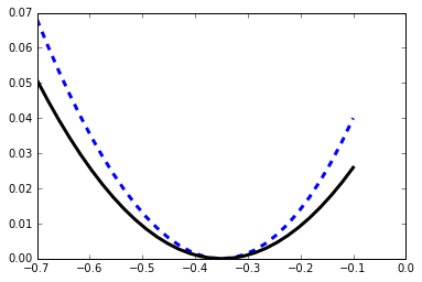
and . Here again, the moderate rate function turns out to be the second-order Taylor expansion of the large deviations rate function at its minimum. More precisely, it is easy to show that attains its minimum at , which corresponds to the limiting behaviour (at ) of as tends to zero. Indeed, due to ergodicity, we have that . We can also show that , where the constant is given by the moderate deviations regime (17). Hence, the moderate deviations rate function characterizes the local curvature of the large deviations rate function around its minimum.
4. Limiting behaviour for integrated functionals
We now consider an extension of the previous results to functionals of diffusion processes, and prove moderate deviations thereof. This problem has already been approached in [22], but, using weak convergence techniques, we are able to relax some of the their assumptions, making the results amenable to applications in mathematical finance, see also Remark 4.6. We consider the model
| (18) |
which corresponds to the original system (1) using the general rescaling (2) (as in the large-time framework above), whenever the coefficients do not depend on . For given sets , for and we denote by , the space of functions with bounded derivatives in and derivatives in , with all partial derivatives being -Hölder continuous with respect to , uniformly in . For any , let denote the infinitesimal generator of the process when (i.e. before the space/time rescalings):
| (19) |
and let be the invariant measure corresponding to the infinitesimal generator , which is guaranteed to exist by Assumption 4.1 below. With
| (20) |
let us set
It is a classical result [29] that converges in probability to as tends to zero, where
| (21) |
For an appropriate function , let ; we are interested in the LDP for
| (22) |
The following assumption is a counterpart to Assumption 3.1 in the more general configuration with full dependence on and in the coefficients.
Assumption 4.1.
-
(i)
There is such that either and , or and .
-
(ii)
There exist constants and such that
In addition, is Lipshitz continuous in locally uniformly with respect to .
-
(iii)
We can write with , is a globally Lipschitz function in , uniformly with respect to , with Lipschitz constant , and for large enough.
-
(iv)
The function is either uniformly continuous and bounded from above and away from zero or alternatively it takes the form for and a non-zero constant. In the latter case we also assume that .
-
(v)
There exist constants and such that
Assumption 4.2.
The SDE (18) has a unique strong solution.
Let us further consider to be the solution to the Poisson equation
| (23) |
By Theorem A.1 and Lemma A.2, is a well-defined classical solution that can grow at most polynomially in . Next, due to compactness issues, that we will see in the proof of tightness in Section 7.1, we need to restrict the values of the constants that dictate the growth in of the coefficients , and respectively. We collect these constraints in the following assumption:
Assumption 4.3.
Notice that for Assumption 4.3(ii), if , then assuming with yields , so that Assumption 4.3 is satisfied if and only if . In order to state the main result, we shall need one additional assumption, merely for technical reasons. Given the solution to the Poisson equation (23) and the constant defined in (20), introduce the following:
| (25) |
Assumption 4.4.
The Lebesgue measure of the set is equal to zero.
At this point, we mention that the reason we single out the operator (24) is because in this case we can have more detailed information on the behaviour of the solutions to the corresponding Poisson equation (23). This is discussed in detail in Lemma A.2. To be specific, in the special case of (24) with , the solution to the PDE (23) grows like whereas the derivative grows like for . On the other hand, in the general case, one can only guarantee that both solution and derivatives to the solution of PDE (23) grow like . Then, we have the following result, proved in Sections 6-7:
Theorem 4.5.
Remark 4.6.
We point out that a result similar to Theorem 4.5 has also been established in [22] using different methods. However, the results of [22] are not sufficient for our purposes, as they assumed that both functions and are bounded ( is even assumed to be bounded by for some ). In our work we allow the coefficients to grow according to Assumptions 4.1 and 4.3. In turn this allows us to consider a considerably wider class of models. We see some examples below.
5. Financial applications: asymptotic behaviour of option prices
We can use Corollary 2.5 for the short-time asymptotics and Theorem 3.3 for the long-time asymptotics to get statements for Call option prices analogous to Theorem 6.2 and 6.3 of [17]. Theorem 4.5 is used to obtain estimates on asymptotics for realised variance.
5.1. Tail estimates
We show here how the general result in Theorem 2.3, as well as its lighter versions in Proposition 2.4 and Corollary 2.5 yield, for some suitable scaling, tail estimates for probabilities. We shall consider the following forms for the coefficients of the SDE (6):
Assumption 5.1.
There exist , together with and such that
These assumptions may look restrictive, but are in fact sufficient for many financial applications, as detailed further below. Note that we excluded the trivial case as the SDE for is then independent of , and can be dealt with directly by hand.
Proposition 5.2.
Proof.
Let to be chosen. Under Assumption 5.1, the model (6) reads
with starting point . The rescaling for all yields the system
with starting point . Equating the powers in the diffusion coefficients yields , or , so that
with . Setting finally gives the system
with starting point . Theorem 2.3 then applies whenever and , which is equivalent to , and the proposition follows by setting . ∎
5.2. Small-time behaviour
The following theorem is a reformulation of [17, Theorem 6.3] and [12, Corollary 2.1 and Theorem 2.2], based on the asymptotic behaviour (assuming for simplicity)
| (26) |
as tends to zero, from Proposition 2.4 and Corollary 2.5, with . This behaviour in fact follows directly from our main result above; in the model (6), the pathwise moderate deviations principle for the first component (Corollary 2.5) generalises (being pathwise and with weaker assumptions) the results from [17], and directly yields (26). More precisely, from the proposed scaling , Corollary 2.5 and Remark 2.6 imply, as tends to zero, for ,
which in turn implies (26), identifying to and setting . In order to state the main result here, we need the following assumption:
Assumption 5.4.
For any there exists such that is finite for all .
Remark 5.5.
The moment assumption in the theorem is classical in the mathematical finance literature related to large and moderate deviations for option pricing. It can be found in [17, Theorem 6.3] and in the more general framework [15, Assumption (A2)]. Essentially, this assumption ensures that some integrability of the stock price is guaranteed (otherwise Call prices may not be defined), which is not automatically granted by large and moderate deviations results. We refer the reader to [15, Lemma 4.7] for some easy-to-check condition.
Proof.
We follow here the proof of [17, Theorem 6.3] with minor modifications. In the small-maturity case, the limiting process is equal to , so that Corollary 2.5 and Remark 2.6 imply that, as tends to zero, and identifying to ,
For any , there exists then such that for all , letting ,
where the constant is of no importance. Letting , the Call price reads
Regarding the first term, we can write
The second term is dealt with from the moderate deviations principle with replaced by :
and therefore
Letting tends to zero yields the desired lower bound. Regarding the upper bound, fix and note that, by Assumption 5.4, is finite for all . Doob’s inequality [25, Theorem 3.8], implies
where , so that also has finite -th moment, and
By dominated convergence and since the process has continuous paths, then converges to as tends to zero. Finally, for any such that , Hölder’s inequality yields
Since the first term converges to , we then obtain
Letting tend to infinity, and consequently to one, yields the lower bound in the theorem. ∎
5.3. Large-time behaviour
Following the methodology developed in [13, 24], we can translate the moderate deviations results into large-time asymptotic behaviours of option prices. In order to state the results, let denote the (convex) contraction of the rate function given in Theorem 3.3 onto the last point, i.e. . Introduce further the Share measure for any . Before proving the main result of this section, let us state and prove a useful lemma.
Lemma 5.7.
Proof.
From (10), we can write
where we decomposed the Brownian motion into . Girsanov’s Theorem implies that the two processes and defined as
are two independent standard Brownian motions under , and we can rewrite (10) as (27) with and . The lemma then follows directly from Theorem 3.3 under the assumptions on the coefficients. ∎
Note the flipped sign in the drift of in (27). We can thus define as the contraction (onto the last point) of the rate function for under . The minimising functional in Theorem 3.3 is linear, of the form , hence
| (28) |
Proposition 5.8.
Let . As tends to infinity, we observe the following asymptotic behaviours:
Proof.
We follow the methodology developed in [24, Theorem 13] with a few changes. For all and , the inequalities
hold. Taking expectations, logarithms and dividing by , we obtain
From the moderate deviations principle in Theorem 3.3 and using (28), we can write
so that, as tends to infinity, the asymptotic behaviour for Put option prices in the proposition holds.
5.4. Asymptotics of the realised variance
We now show how Theorem 4.5 applies to the realised variance in the Heston model (9). The rescaling (2) yields the same perturbed system (15) as in the large-time case. Likewise, the invariant measure has Gamma density given in (16). With , we have and , so that Assumption 4.3 holds and Theorem 4.5 gives the pathwise large deviations for the process
| (29) |
In this case, the Poisson equation (23) satisfies , and hence , yielding the rate function
| (30) |
Take for simplicity , i.e. , then we can write, for any ,
where we denote , and represents the realised variance over the period . The large deviations for the sequence therefore implies that, taking , and applying the contraction principle, for any fixed ,
or, taking for example for , and renaming ,
Here again, this minimum can be computed in closed form from (30). The corresponding Euler-Lagrange equation yields the linear optimal path , for any , so that
Note that, since the drift and diffusion of in (9) do not depend on itself, then is constant here. In the Heston case (9), we can compare this large-time MDP to the corresponding large-time LDP for the realised variance. Indeed, from [4, Proposition 6.3.4.1], the moment generating function for the realised variance reads, for all such that the right-hand side is finite,
where . Straightforward computations yield that
We can therefore use a partial version of the Gärtner-Ellis theorem [7, Section 2.3] to show that the sequence satisfies a large deviations principle as tends to infinity, with rate function defined as the Fenchel-Legendre transform of . More precisely, for any ,
Again, we observe that the moderate deviations rate function characterises the local curvature of the large deviations rate function around its minimum. We can translate this behaviour into asymptotics of options on the realised variance, both in the large deviations case and in the moderate deviations one:
Proposition 5.9.
Let . As tends to infinity, we have, for all ,
Remark 5.10.
Note that, again, formally setting in the second limit, which arises from moderate deviations, one obtains after simplification,
which again, as in Remark 3.6, indicates that the moderate deviations rate function represents exactly the curvature of the large deviations one at its minimum.
Proof.
We start with the first limit, which falls in the scope of large deviations. Mimicking the proof of Proposition 5.8, for all and , we can write the inequalities
Taking expectations, logarithms and dividing by and taking limits, we obtain
The large deviations obtained above for the sequence as tends to infinity concludes the proof.
We now prove the other limit, which arises from moderate deviations. Now, mimicking the proof of Proposition 5.8, for all and , we can write
with , so that, taking expectations, logarithms and dividing by , the proposition follows from
∎
6. Control representations for the proof of Theorem 4.5
In this section we connect Theorem 4.5 to certain stochastic control representation and to the Laplace principle. We start by applying Itô formula to the solution to (23). Rearranging terms, we obtain
We shall consider through this expression together with (18) as the triple . By [10, Section 1.2], the large deviations principle (with speed ) for is equivalent to the Laplace principle, which states that for any bounded continuous function mapping to ,
| (31) |
where is called the action functional. We prove (31) and then Theorem 4.5 identifies . The proof of (31) is based on appropriate stochastic control representations developed in [3]. Let be the space of -progressively measurable two-dimensional processes such that is finite. From [3, Theorem 3.1], we can write the stochastic control representation
| (32) |
where the controlled process satisfies the system
| (33) | ||||
with . With this control representation at hand, we proceed by analysing the limit of the right-hand side of (32) as tends to zero. Similarly to [28], we define the function by
| (34) |
Let define the control space, and the state space of . Our assumptions guarantee that is bounded in , affine in growing at most polynomially in . Next step is to introduce an appropriate family of occupation measures whose role is to single out the correct averaging taking place in the limit. For this reason, let be a parameter whose role is to exploit a time-scale separation. Let , , , be Borel sets of , , , respectively. Then, define the occupation measure by
| (35) |
and assume if . For a Polish space , let be the space of probability measures on . Next we recall the definition of a viable pair for the moderate deviations case.
Definition 6.1 (Definition 4.1 in [28]).
Let be a function that grows at most linearly in . For each , let be a second-order elliptic partial differential operator and denote by its domain of definition. A pair is called a viable pair with respect to , and we write , if
-
•
the function is absolutely continuous;
-
•
the measure is integrable in the sense that
-
•
for all (with defined in (21)),
(36) -
•
for all and for every ,
(37) -
•
for all ,
(38)
The last item is equivalent to stating that the last marginal of is Lebesgue measure, or that can be decomposed as . Then we shall establish the following result:
Theorem 6.2.
7. Proof of Theorem 4.5
In this section we offer the proof of Theorem 4.5. As mentioned in Section 6, the proof of Theorem 4.5 is equivalent to that of the Laplace principle in Theorem 6.2. In Subsections 7.1 and 7.2 we prove tightness and convergence of the pair respectively. In Subsection 7.3, we finally establish the Laplace principle and the representation formula of Theorem 4.5. The proofs of these results make use of the results of [28]. Below we present the main arguments, highlighting the differences and give exact pointers to [28] when appropriate.
7.1. Tightness of the pair
In this section we prove the following proposition:
Proposition 7.1.
Proof of Proposition 7.1.
Tightness of on and the uniform integrability of the family of occupation measures is the subject of [28, Section 5.1.1], and will not be repeated here. It remains to prove tightness of on . We prove it making use of the characterisation of [2, Theorem 8.7], and it follows if we establish that there is such that for every ,
-
(i)
there exists such that
(40) -
(ii)
for every ,
(41)
Essentially both statements follow from the control representation (6) together with the results on the growth of the solution to the Poisson equation by Theorem A.1 and Lemma A.2 and using Lemma B.5 to treat each term on the right-hand side of (6). For sake of completeness, we prove the first statement (40). The second statement (41) follows similarly using the general purpose Lemma B.5. Rewrite (6) as
| (42) |
where represents the term on the right-hand side of (6), and notice that
Theorem A.1 and an application of Hölder inequality imply that, for ,
| (43) |
where the third inequality follows from Lemma B.4. This certainly stays bounded (actually, it goes to zero) by Assumption 4.3 and because, for any we can choose so that . Hence we obtain that for some unimportant constant ,
For the stochastic integral term , we have that for a constant that may change from line to line and for small enough such that (with some abuse of notation is the degree of polynomial growth in of the function ), we have
from which the result follows by Lemma B.5 given that . Similarly, we obtain a corresponding bound for the other stochastic integral term . The Riemann integral terms are treated very similarly again using Lemma B.5. The conditions on and from Assumption 4.3 guarantee that Lemma B.5 applies in these cases. These considerations yield (40).
The second statement (41) follows by similar arguments using again Lemma B.5 and the growth properties of the involved functions with respect to . The only term that potentially needs some discussion is the term. In particular, we need to show that for every , there exists such that
But this follows again by the estimate on above together with Assumption 4.3. This completes the proof of the proposition. ∎
7.2. Convergence of the pair
In Section 7.1 we proved that the family of processes is tight. It follows that for any subsequence of converging to 0, there exists a subsubsequence of which converges in distribution to some limit . The goal of this section is to show that is a viable pair with respect to , according to Definition 6.1. To show that the limit point is a viable pair, we must show that it satisfies (36), (37), and (38). The proof of (37) and (38) can be found in [28, Section 5.2], whereas the proof of statement (36) follows via the Skorokhod Representation Theorem [2, Theorem 6.7] and the martingale problem formulation. For completeness, we present the argument below. We will invoke the Skorokhod Representation Theorem, which allows us to assume that there exists a probability space in which the desired convergence occurs with probability one. Let us define
As in the proof of (43),
so that it is enough to consider the limit in distribution of the family . The rest of the argument is now classical.
Consider an arbitrary function that is real valued, smooth with compact support on . Fix two positive integers and and let , , be real valued, smooth functions with compact support on . Let , , and , , be nonnegative real numbers with . Let be a real-valued, bounded and continuous function with compact support on . Given a measure and , define
the empirical measure
as well as the operator as
Based on the martingale problem formulation, proving (36) is equivalent to proving that
| (44) |
and
| (45) |
Note first that for every real-valued, continuous function with compact support and , converges to with probability one as tends to zero. Now (45) follows directly by the first statement of [28, Lemma 5.1]. In order to prove (44) we first apply the Itô formula to . Then it is easy to see that all of the terms apart from
in the representation (42) will vanish in the limit. This term surviving in the limit together with the second statement of [28, Lemma 5.1] directly yield (44). This concludes the proof of (36).
7.3. Laplace principle and compactness of level sets
We prove here the Laplace principle lower and upper bounds and the compactness of level sets of the action functional . We start with the lower bound, i.e. we need to show that for all bounded, continuous functions mapping into ,
It is sufficient to prove it along any subsequence such that converges, which exists due to the uniform bound on the test function . In addition, by Lemma B.1, we may assume that
for some constant . For such controls, we construct the family of occupation measures from (35), and per Proposition 7.1 the family is tight. This indicates that for any subsequence, there is a further subsequence for which converges to in distribution, with being a viable pair per Definition 6.1. Then using Fatou’s lemma, we conclude the proof of the lower bound
Next we want to prove compactness of level sets. Namely, we want to show that for each , the set is a compact subset of , which amounts to showing that it is precompact and closed. The proof is analogous to the proof of the lower bound using Fatou’s lemma on the form of as given by (39) and thus the details are omitted; see also [11] for further details.
It remains to show the upper bound. From [28] we can write , where
Then, applying [28, Theorem 5.1] we get that if defined in (25) is non-degenerate everywhere then
| (46) |
and the infimum is attained at
This representation essentially gives the equivalence between Theorems 4.5 and 6.2. Now, we have all the tools needed to prove the Laplace principle upper bound. We need to show that for all bounded, continuous functions mapping into ,
Let be given and consider with such that
Since is bounded, this implies that is finite, and thus is absolutely continuous. Because is continuous and finite at each , a mollification argument allows us to assume that is piecewise continuous, as in [10, Section 6.5]. Given this define
Define a control in feedback form by
Then converges to in distribution, where
with probability one. If becomes zero at a countable number of points, we define if and otherwise (recall Assumption 4.4). At the same time, the cost satisfies
In addition, the relation (46) implies that
Then, we can finally write
Since is arbitrary, the upper bound is proved. The proof also shows that we have the explicit representation given by Theorem 4.5.
Appendix A Regularity results on Poisson equations
Theorem A.1.
Under Assumption 4.1, set . If there exist such that
then there is a unique solution from the class of functions which grow at most polynomially in to
Moreover, the solution satisfies for every , , and there exists such that
While Theorem A.1 addresses regularity and growth properties of solutions to general Poisson equations, Lemma A.2 specialises the discussion on Poisson equations whose operators correspond to the so-called CEV model—widely used in mathematical finance—and where the right-hand side is only a function of . In this case, we have more precise information on the growth of the solution and its derivatives.
Lemma A.2.
Proof.
If the generator corresponds to the CIR model, i.e., when , we refer the reader to [19, Lemma 3.2]. We prove it for the more general case and using a more direct argument. The invariant measure has density given by the speed measure of the diffusion:
and a quick computation shows that the derivative to the solution of the Poisson PDE satisfies
where we used the centering condition to obtain the last equality. Now, without loss of generality we assume that . For some positive constant that may change from line to line, we can write
with and . Since , the function is smooth and strictly increasing on . Furthermore, since , the function is smooth on . As becomes large, this integral is exactly of Laplace type, albeit without a saddlepoint for , its minimum being attained at the left boundary of the domain. Using [27, Section 3.3], we can write, for large ,
and therefore, as tends to infinity, , and the lemma follows. ∎
Remark A.3.
It is clear from the proof of Lemma A.2 that its statement is also true in the case of with (the drift component in the operator ) growing at most linearly in .
Appendix B Preliminary results on the involved controlled processes
In this section we recall some results from [28] and we prove some additional corollaries related to certain bounds involving the controlled processes (6) appearing via the weak convergence control representation.
Lemma B.1 (Lemma B.1 of [28]).
Lemma B.2 (Lemma B.2 of [28]).
Lemmas B.3-B.4 follow from Lemma B.2, but since their proof was not included in [28], we include them here.
Lemma B.3.
Proof of Lemma B.3.
For notational simplicity, let us set . By the factorization argument (see for example page 229 of [6]), we have that for any , there is a constant such that
where
Then for any we get
By the Burkholder-Davis-Gundy inequality, we get
Using the inequality that for any ,
we obtain
Therefore, we get
Next choosing and we get by Young’s inequality
Then, by Lemma B.2, if we choose (which is possible since and ) we obtain for some constant
Putting the latter bounds together, we then obtain for some constant independent of :
Gathering together all the restrictions on , we have that we need , which due to the relation means that . Then the restriction gives that .
Then, for we get for some unimportant constant that may change from line to line
competing the proof of the lemma. ∎
Lemma B.4.
Proof of Lemma B.4.
By Assumption 4.1, we can write that , and we can assume that is globally Lipschitz in with Lipschitz constant , where is from Assumption 4.1. For presentation purposes and without loss of generality, we only prove the case , i.e., when the Brownian motions are independent. It is easy to see that
where
Let us also set , so that
Hence, we have
for some unimportant positive constant . In the last line we used the Lipschitz and growth properties of together with Young’s inequality. Then we obtain that for some finite constant ,
We now bound each term separately. We have for some constant that may change from line to line
Using now Lemma B.3, we have that for any ,
Consequently, we obtain that for some appropriate constant ,
Hence, recalling the original definition of , we have for small enough such that and for some constant that changes from line to line,
where in the last step we used Young’s generalised inequality. Hence, by rearranging terms we obtain
completing the proof of the lemma. ∎
References
- [1] D. Baier and M. I. Freidlin. Theorems on large deviations and stability for random perturbations. Dokl. Akad. Nauk SSSR 235: 253-256, 1977.
- [2] P. Billingsley. Convergence of Probability Measures, Second Edition, Wiley, New York, 1968.
- [3] M. Boué and P. Dupuis. A variational representation for certain functionals of Brownian motion. Annals of Probability, 26(4): 1641-1659, 1998.
- [4] M. Chesney, M. Jeanblanc and M. Yor. Mathematical methods for financial markets. Springer-Verlag London, 2009.
- [5] A. Chiarini and M. Fischer. On large deviations for small noise Itô processes. Advances App. Prob., 46: 1126-1147, 2014.
- [6] G. Da Prato and J. Zabczyk. Stochastic Equations in Infinite Dimensions. Encyclopedia of Mathematics and its Applications. Cambridge University Press, 2008.
- [7] A. Dembo and O. Zeitouni. Large deviations techniques and applications. Springer-Verlag New-York, 1998.
- [8] J.D. Deuschel, P.K. Friz, A. Jacquier and S. Violante. Marginal density expansions for diffusions and stochastic volatility, Part I: Theoretical foundations. Communications on Pure and Applied Mathematics, 67(1): 40-82, 2014.
- [9] J.D. Deuschel, P.K. Friz, A. Jacquier and S. Violante. Marginal density expansions for diffusions and stochastic volatility, Part II: Applications. Communications on Pure and Applied Mathematics, 67(2): 321-350, 2014.
- [10] P. Dupuis and R.S. Ellis. A weak convergence approach to the theory of large deviations. John Wiley & Sons, New York, 1997.
- [11] P. Dupuis and K. Spiliopoulos. Large deviations for multiscale problems via weak convergence methods. Stochastic Processes and their Applications, 122: 1947-1987, 2012.
- [12] J. Feng, J.-P. Fouque and R. Kumar. Small-time asymptotics for fast mean-reverting stochastic volatility models. Annals of Applied Probability, 22(4): 1541-1575, 2012.
- [13] M. Forde and A. Jacquier. The large-maturity smile for the Heston model Finance and Stochastics, 15(4): 755-780, 2011.
- [14] M. Freidlin. The averaging principle and theorems on large deviations. Russian Math. Surveys, 33(5): 117-176, 1978.
- [15] P. Friz, P. Gassiat and P. Pigato. Precise asymptotics: robust stochastic volatility models. Preprint arXiv: 1811.00267, 2018.
- [16] P. Friz, J. Gatheral, A. Gulisashvili, A. Jacquier and J. Teichmann. Large deviations and asymptotic methods in finance. Springer Proceedings in Mathematics and Statistics, 110, 2015.
- [17] P. Friz, S. Gerhold and A. Pinter. Option pricing in the moderate deviations regime. Forthcoming in Mathematical Finance.
- [18] P. Friz, S. Gerhold and M. Yor. How to make Dupire’s local volatility work with jumps. Quant. Fin., 14(8): 1327-1331, 2014.
- [19] J.-P, Fouque, G. Papanicolaou, R. Sircar and K. Solna. Multiscale stochastic volatility for equity, interest rate, and credit derivatives. Cambridge University Press, Cambridge, 2011.
- [20] A. Guillin. Averaging principle of SDE with small diffusion: moderate deviations. Annals of Probability, 31(1): 413-443, 2003.
- [21] A. Guillin and R. Liptser. Examples of moderate deviation principle for diffusion processes. Discrete and Continuous Dynamical Systems (B), 6(4): 803-828, 2006.
- [22] A. Guillin and R. Liptser. MDP for integral functionals of fast and slow processes with averaging. Stochastic Processes and their applications, 115: 1187-1207, 2005.
- [23] A. Gulisashvili and E. Stein. Asymptotic behavior of the stock price distribution density and implied volatility in stochastic volatility models. Applied Mathematics and Optimization, 61(3): 287-315.
- [24] A. Jacquier, M. Keller-Ressel and A. Mijatović. Large deviations and stochastic volatility with jumps. Stochastics, 85(2): 321-345, 2013.
- [25] I. Karatzas and S. Shreve. Brownian Motion and Stochastic Calculus. Springer, 1991.
- [26] R. Lipster and V. Spokoiny. Moderate deviations type evaluation for integral functional of diffusion processes. Electronic Journal of Probability, 4: 1-25, 1999.
- [27] P.D. Miller. Applied asymptotic analysis. Graduate Studies in Mathematics, 75, AMS, 2006.
- [28] M. Morse and K. Spiliopoulos. Moderate deviations principle for systems of slow-fast diffusions. Asymptotic Analysis, 105: 97-135, 2017.
- [29] E. Pardoux and A.Yu. Veretennikov. On the Poisson equation and diffusion approximation I. Annals of Probability, 29(3): 1061-1085, 2001.
- [30] E. Pardoux and A.Yu. Veretennikov. On Poisson equation and diffusion approximation II. Annals of Probability, 31(3): 1166-1192, 2003.
- [31] S. Robertson. Sample path large deviations and optimal importance sampling for stochastic volatility models. Stochastic Processes and their Applications, 120(1), 66-83, 2010.
- [32] K. Spiliopoulos. Large deviations and importance sampling for systems of slow-fast motion. Applied Mathematics and Optimization, 67: 123-161, 2013.
- [33] E. Stein and J. Stein. Stock price distributions with stochastic volatility: an analytic approach. Review of Financial Studies, 4(4): 727-752, 1991.