Poisson Kernel-Based Clustering on the Sphere: Convergence Properties, Identifiability, and a Method of Sampling

Abstract

Many applications of interest involve data that can be analyzed as unit vectors on a d-dimensional sphere. Specific examples include text mining, in particular clustering of documents, biology, astronomy and medicine among others. Previous work has proposed a clustering method using mixtures of Poisson kernel-based distributions (PKBD) on the sphere. We prove identifiability of mixtures of the aforementioned model, convergence of the associated EM-type algorithm and study its operational characteristics. Furthermore, we propose an empirical densities distance plot for estimating the number of clusters in a PKBD model. Finally, we propose a method to simulate data from Poisson kernel-based densities and exemplify our methods via application on real data sets and simulation experiments.

Keywords: directional data, empirical densities distance plot, generalized quadratic distance, mixture models, Poisson kernel, rejection sampling.

1 Introduction

Directional data arise naturally in many scientific fields where observations are recorded as directions or angles relative to a fixed orientation system. Directions may be regarded as points on the surface of a hypersphere, thus the observed directions are angular measurements. Directional data are often met in astronomy, where the origin of comets is investigated or in biology, where clustering of gene expression measurements that are standardized to have mean zero and variance 1 across arrays is of interest. Jammalamadaka et al. (1986) discuss a problem in medicine where the angle of knee flexion was measured to assess the recovery of orthopaedic patients. Furthermore, Peel et al. (2001) discuss the analysis of directional data in an application in the mining industry, where a mine tunnel is modeled.

Conventional methods suitable for the analysis of linear data cannot be applied for directional data due to its circular nature. The statistical methods that are used to handle such data are given in several references such as Watson (1983); Fisher (1996); Mardia and Jupp (2000); Lee (2010). Clustering methods for directional data have been developed in the literature. Some commonly used non-parametric approaches are K-means clustering (Ramler, 2008; Maitra and Ramler, 2010), spherical K-means (Dhillon and Modha, 2001), and online spherical K-means (Zhong, 2005). Furthermore, some of the clustering methods proposed in the literature are appropriate for small and medium dimensional data sets, while high dimensional data are considered in Dryden (2005); Banerjee et al. (2003, 2005); Zhong and Ghosh (2003, 2005), with applications to brain shape modeling, text data represented by large sparse vectors, and genomic data.

Probability models have been proposed for quite sometime as a basis for cluster analysis. In this approach the data are viewed as generated from a mixture of probability distributions, each representing a different cluster. Clustering algorithms based on probability models allow uncertainty in cluster membership, and direct control over the variability allowed within each cluster. Probabilistic approaches are also called generative approaches and a list of references on these approaches in the context of clustering text can be found in Zhong and Ghosh (2003, 2005) and Blei et al. (2003). Banerjee et al. (2005) considered a finite mixture of von Mises-Fisher (vMF) distributions to cluster text and genomic data. The spherical k-means algorithm, has been shown to be a special case of a generative model based on a mixture of vMF distributions with equal priors for the components and equal concentration parameters (Banerjee and Ghosh, 2002; Banerjee et al., 2003). A comparative study of some generative models based on the multivariate Bernoulli, multinomial distributions, and the generative model based on a mixture of vMF distributions is presented in Zhong and Ghosh (2003).

Golzy et al. (2016), presented a clustering algorithm based on mixtures of Poisson kernel-based distributions (PKBD). Poisson kernels on the sphere (Lindsay and Markatou, 2002) have important mathematical and physical interpretation. A clustering algorithm was devised and estimates of the parameters of the Poisson kernel-based algorithm were obtained in an Expectation-Maximization (EM) setting. Experimental and simulation results indicated that the method performs at least equivalently to the mixture of vMF distributions, which is considered to be the state of the art, and outperforms the aforementioned algorithm in certain data structures, when performance is measured by macro-precision and macro-recall.

In this paper, we present a detailed study of our clustering algorithm, investigate its properties and illustrate its performance. Specifically, our contributions are as follows. First, we study the connection between PKBD and other spherical distributions. Section 3.2 presents the results of the aforementioned study. Section 4 of the paper establishes the identifiability of a mixture model of Poisson kernel-based densities, a new contribution in establishing validity of our PKBD algorithm. Section 5 establishes the convergence of our proposed algorithm, while section 6 discusses a method of sampling from a PKBD family. Practical issues of implementation of our algorithm such as study of the role of initialization on the performance of the algorithm, stopping rules and a method for estimating the number of clusters when data are generated from a mixture of PKBD distributions are discussed in section 7. Section 8 presents experimental results that illustrate the performance of our algorithm, while section 9 offers discussion and conclusions. The online supplemental material associated with the paper contains detailed proofs of our theoretical results and additional simulations, illustrating further the performance of the algorithm. The code and data sets are also provided in the online supplement.

2 Literature Review

In this section, we briefly review the clustering literature for directional data. We, very briefly, refer to algorithms that are distance or similarity based (non-generative algorithms) while our focus is on probabilistic (or generative) algorithms. We begin with a brief description of non-generative algorithms for directional data.

K-means clustering (Duda and Hart, 1973) is one of the most popular methods for clustering. Given a set ${\cal X}$ of $N$ observations, where each observation is a $d$-dimensional real vector, K-means clustering partitions the $N$ observations into $M(\leq N)$ sets ${\cal X}_{1},\cdots,{\cal X}_{M}$ by minimizing the within-cluster sum of squares. Spherical K-means (Dhillon and Modha, 2001), uses cosine similarity instead of Euclidean distance, that measures the cosine of the angle formed by two vectors. Spherical K-means algorithm is preferred to standard K-means for clustering of document vectors or any type of high-dimensional data on the unit sphere, and it is sensitive to initialization and outliers.

Maitra and Ramler (2010) propose a K-means directions algorithm for fast clustering of data on the sphere. They modified the core elements of Hartigan and Wong (1979) efficient K-means implementation for application to spherical data. Their algorithm incorporates the additional constraint of orthogonality to the unit vector, and thus extends to the situation of clustering using the correlation metric.

2.1 Parametric Mixture Model Approach for Clustering

The parametric mixture model assumes each cluster is generated by its own density function that is unknown. The overall data is modeled as a mixture of individual cluster density functions. In practice, the unknown densities may not be from the same family of distributions. In this section, we consider mixture models in which the densities are from the same family of distributions. The probability density function of a mixture with $M$ components on the hypersphere $S^{d-1}$, the unit sphere, is given by

$$f({\bf x}|\Theta)=\sum_{j=1}^{M}\alpha_{j}f_{j}({\bf x}|\mbox{\boldmath$\theta$}_{j}),$$ (1)

where $M$ is the number of clusters, $\alpha_{j}$’s are the mixture proportions that are non-negative and sum to one and $\Theta=(\alpha_{1},\cdots,\alpha_{M},\mbox{\boldmath$\theta$}_{1},\cdots,\mbox{\boldmath$\theta$}_{M})$.

Banerjee et al. (2005) discuss clustering based on mixtures of von Mises-Fisher (vMF) distributions on a hypersphere. Given $\mbox{\boldmath$\mu$}\in S^{d-1},$ and $\kappa\geq 0$, the vMF probability distribution function is defined by $f({\bf x}|\mbox{\boldmath$\mu$},\kappa)=c_{d}(\kappa)e^{\kappa\mbox{\boldmath$\mu$}{\bf\cdot}{\bf x}},$ where $\mu$ is a vector orienting the center of the distribution, $\kappa$ is a parameter to control the concentration of the distribution around the vector $\mu$ and ${\bf y}{\bf\cdot}{\bf x}$ denote the dot product of the vectors. The normalizing constant $c_{d}(\kappa)$ is given by $c_{d}(\kappa)=\frac{\kappa^{d/2-1}}{(2\pi)^{d/2}I_{d/2-1}(\kappa)},$ where $I_{r}(.)$ represents the modified Bessel function of the first kind of order $r$. The vMF distribution is unimodal and symmetric about $\mu$.

Banerjee et al. (2005) performed Expectation Maximization (EM) (Dempster et al., 1977; Bilmes, 1997) for a finite vMF mixture model to cluster text and genomic data. The numerical estimation of the concentration parameter involves functional inversion of the ratios of Bessel functions. Thus, it is not possible to directly estimate the $\kappa$ values in high dimensional data and an asymptotic approximation of $\kappa$ is used for estimating $\kappa$. The package movMF in R software can be used for fitting a mixture of vMF distribution (Hornik and Gr$\ddot{\rm u}$n 2014).

Mixtures of Watson distributions are discussed in Bijral et al. (2007) and Sra and Karp (2013). Given $\mbox{\boldmath$\mu$}\in S^{d-1}$ and $\kappa$, the probability function of a Watson distribution is defined by $f({\bf x}|\mbox{\boldmath$\mu$},\kappa)=M(1/2,d/2,\kappa)^{-1}e^{\kappa(\mbox{\boldmath$\mu$}{\bf\cdot}{\bf x})^{2}},$ where $M(1/2,d/2,\kappa)$ is the confluent hyper-geometric function also known as Kummer function. The advantage of using the class of Watson distributions in the mixture model is that it shows superior performance, when the measure of performance is the mutual information between cluster assignment and preexisting labels, for noisy, thinly spread clusters over the vMF distributions (Bijral et al., 2007). The disadvantage is that in high-dimensions, maximum likelihood equations pose severe numerical challenges. Similar to vMF, it is not possible to directly estimate the $\kappa$ values, since the numerical estimation of $\kappa$ involves a ratio of Kummer functions, and hence an asymptotic approximation for estimating $\kappa$ is used.

Dortet-Bernadet and Wicker (2008) have presented model based clustering of data on the sphere by using inverse stereographic projections of multivariate normal distributions. Recall that, given a direction $\mu$ on the sphere $S^{d-1}$, the corresponding stereographic projection of a point ${\bf x}$ that belongs to $S^{d-1}$ lies at the intersection of a line joining the ”antipole” $-\mbox{\boldmath$\mu$}$ and ${\bf x}$, with a given plane perpendicular to $\mu$. Let ${\cal L}_{\mu,\Sigma}$ denote the distribution on the sphere $S^{d-1}$, which corresponds to the image via an inverse stereographic projection of a multivariate normal distribution $N_{d-1}({\bf 0},\Sigma)$ that is defined on the plane of dimension $d-1$ perpendicular to $\mu$. The density function of ${\cal L}_{\mu,\Sigma}$ is given by

$$f_{\mu,\Sigma}({\bf x})=\frac{1}{(2\pi)^{(d-1)/2}}|\Sigma|^{-1/2}\exp\{-1/2P(R_{\mu^{-1}}({\bf x}))^{T}\Sigma^{-1}P(R_{\mu^{-1}}({\bf x}))\}\frac{1}{(1+\mbox{\boldmath$\mu$}{\bf\cdot}{\bf x})^{d-1}},$$ (2)

where $P(.)$ is the stereographic projection map and $R_{\mu}(.)$ is the rotation in ${\rm I\!R}^{d}$ such that $R_{\mu}(e_{1})=\mbox{\boldmath$\mu$}$, where $\{e_{1},\cdots,e_{d}\}$ is the canonical basis of the ${\rm I\!R}^{d}$. Given $\mu$, $\hat{\Sigma}_{\mu}=1/n\sum_{i=1}^{n}P(R_{\mu}^{-1}({{\bf x}_{i}}))P(R_{\mu}^{-1}({{\bf x}_{i}}))^{T},$ and $\mbox{\boldmath$\mu$}_{MLE}$ maximizes the expression given by
${\rm Expr}(\mbox{\boldmath$\mu$})=-1/2n\log(|\hat{\Sigma}_{\mu}|)-(p-1)\sum_{i=1}^{n}\log(1+\mbox{\boldmath$\mu$}{\bf\cdot}{\bf x_{i}}).$

The advantage of using the class of inverse stereographic projection of the multivariate normal distribution in the mixture model is that it allows clustering with various shapes and orientations. The projected multivariate normal is applied to a real data set of standardized gene expression profiling. The disadvantage is that, there is no closed expression for $\mbox{\boldmath$\mu$}_{MLE}$. In practice, it is obtained via a heuristic search algorithm.

3 Clustering Based on Mixtures of Poisson Kernel-Based Distributions

We propose a parametric mixture model approach to clustering directional data based on Poisson kernel-based distributions on the unit sphere. Clustering on the basis of Poisson kernel-based densities avoids the use of approximations, obtains closed form solutions and provides robust clustering results.

3.1 Poisson Kernel-Based Distributions (PKBD)

We use Poisson kernel as a density function on the sphere. To provide perspective we note here that the simplest PKBD provided by the univariate Poisson kernel, is a circular distribution that is also known as the wrapped Cauchy distribution. This distribution can be constructed by ”wrapping” the univariate Cauchy distribution around the circumference of the circle of unit radius. It was studied first by Lev́y (1939) and Wintner (1947).

Let ${\rm I\!B}^{d}$ be the open unit ball in ${\rm I\!R}^{d}$ (i.e; ${\rm I\!B}^{d}(0,1)$) and $S^{d-1}$ be the unit sphere, The $d$-dimensional Poisson kernel for the unit ball is defined for $({\bf x},\mbox{\boldmath$\zeta$})\in{\rm I\!B}^{d}\times S^{d-1}$ by

$$P_{d}({\bf x},\mbox{\boldmath$\zeta$})=\frac{1-\big{\|}{\bf x}\big{\|}^{2}}{\omega_{d}\big{\|}{\bf x}-\mbox{\boldmath$\zeta$}\big{\|}^{d}},$$ (3)

where $\omega_{d}=2\pi^{d/2}\{\Gamma(d/2)\}^{-1}$ is the surface area of the unit sphere in ${\rm I\!R}^{d}$. The family of Poisson kernels is the set $\{K_{\rho}({\bf x},{\bf y}):0<\rho<1\}$, where $K_{\rho}({\bf x},{\bf y})$ defined on $S^{d-1}\times S^{d-1}$ by

$$K_{\rho}({\bf x},{\bf y})=P_{d}(\rho{\bf x},{\bf y}).$$ (4)

Let $\sigma$ be the uniform measure on $S^{d-1}$ (so that $\sigma(S^{d-1})=\omega_{d}$), then $\int_{S^{d-1}}K_{\rho}({\bf x},\mbox{\boldmath$\zeta$})d\sigma(\mbox{\boldmath$\zeta$})=1,$ and so $K_{\rho}({\bf x},{\bf y})$ is a density with respect to uniform measure (Axler et al., 2001; Lindsay and Markatou, 2002; Dai and Xu, 2013).

We discuss clustering based on mixtures of Poisson kernel-based distributions (mix-PKBD) on a hypersphere. Given $\mbox{\boldmath$\mu$}\in S^{d-1},$ and $0<\rho<1$, the probability distribution function of a d-variate Poisson kernel-based density is defined by

$$f({\bf x}|\rho,\mbox{\boldmath$\mu$})=\frac{1-\rho^{2}}{\omega_{d}\big{\|}{\bf x}-\rho\mbox{\boldmath$\mu$}\big{\|}^{d}},$$ (5)

where $\mu$ is a vector orienting the center of the distribution, and $\rho$ is a parameter to control the concentration of the distribution around the vector $\mu$. That is, the parameter $\rho$ is related to the variance of the distribution. PKBDs are unimodal and symmetric around $\mu$. Figure 1 shows the shape of Poisson kernel-based densities for various values of the parameter $\rho$. For additional pictorial representation of the PKBDs for various values of $\rho$ see Figure A15 of the supplemental material. We note that

$$\frac{1-\rho}{\omega_{d}(1+\rho)^{d-1}}<f({\bf x}|\rho,\mbox{\boldmath$\mu$})<\frac{1+\rho}{\omega_{d}(1-\rho)^{d-1}}.$$ (6)

Therefore, if $\rho\rightarrow 0$ then $f({\bf x}|\rho,\mbox{\boldmath$\mu$})\rightarrow 1/\omega_{d}$ which is the uniform density on $S^{d-1}$ and if $\rho\rightarrow 1$, $f({\bf x}|\rho,\mbox{\boldmath$\mu$})$ converges to a point density.

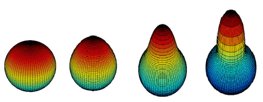
Figure 1: Scaled 3-variant Poisson kernel-based density with $\mbox{\boldmath$\mu$}=(0,0,1)$ and various $\rho$ values.

3.2 Connections with Other Spherical Distributions

In general, given a distribution on the line, Mardia and Jupp (2000) note that we can wrap it around the circumference of the circle of unit radius. If $X$ has distribution $F$ then the wrapped distribution $F_{w}$ of $\theta$ is given by

$$F_{w}(\theta)=\sum_{k=-\infty}^{k=\infty}\{F(\theta+2\pi k)-F(2\pi k)\}{\rm~{}for~{}}0\leq\theta\leq 2\pi,$$ (7)

where $\theta=X\mod 2\pi$. In particular if $\theta$ has density $f$ then $f_{w}(\theta)=\sum_{k=-\infty}^{k=\infty}f(\theta+2\pi k)$ (Mardia and Jupp, 2000).

Mardia and Jupp (2000) note that both wrapped normal and wrapped Cauchy (that is PKBD for d=2) can be use as an approximation of vMF distributions. Figure 2, gives the plots of the two distributions, PKBD (solid line) and vMF (dashed line), with the same mean values and various $\kappa$ and $\rho$ values. The corresponding $\rho$ values are chosen in a way that both distributions have the same maximum. The variable $t$ is the angle between ${\bf x}$ and $\mu$, measured in radian (from -3.14 to 3.14 radians). We note that the PKBD has heavier tails than the vMF distribution. We will illustrate this fact for dimension 4 in the supplemental material (Figure A16). PKBD also has heavier tails than the Elliptically Symmetric Angular Gaussian (ESAG) (Paine et al., 2017) which is a subfamily of Angular Central Gaussian Distribution (ACGD). An illustration is given in the supplemental material (Figure A17). Furthermore, notice that as $\kappa$ increases the value of $\rho$ also increases.

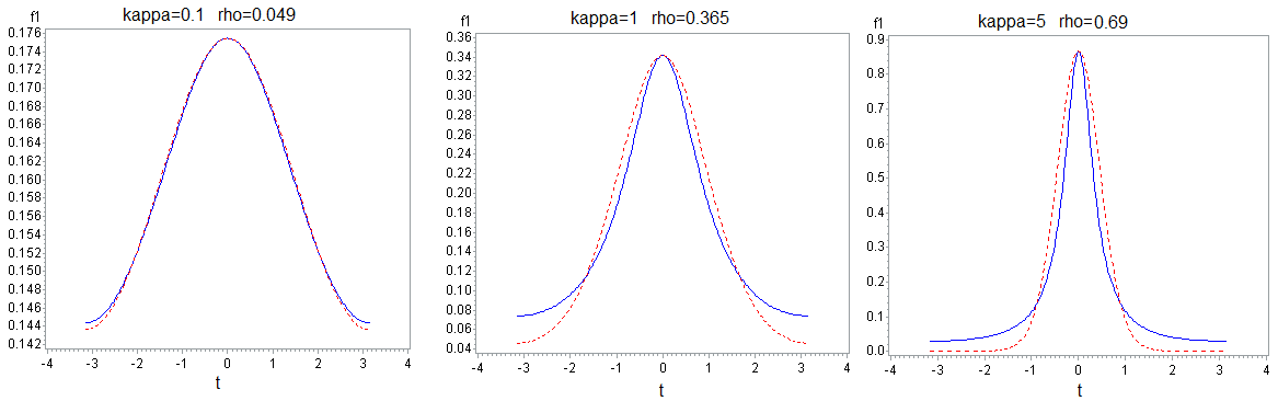
Figure 2: Comparison of the Poisson kernel-based (solid) and von Mises Fisher (dashed) distributions for d=2 with the same maximum values, $t$ is the angle between ${\bf x}$ and $\mu$ measured in radian.

The two dimensional PKBD is also related to projected normal distribution. Let ${\bf y}=(y_{1},\cdots,y_{d})\sim N_{d}(\mbox{\boldmath$\mu$},\Sigma)$ with $P({\bf y}=0)=0$ then ${\bf u}={\bf y}/|{\bf y}|$ is a random variable in $S^{d-1}$. The random variable ${\bf u}$ has a projected normal distribution denoted by ${\bf u}\sim PN_{d}(\mbox{\boldmath$\mu$},\Sigma)$. In the special case where $\mbox{\boldmath$\mu$}=0$, the density of ${\bf u}$ is given by

$$f({\bf u}|\mbox{\boldmath$\mu$}=0,\Sigma)=\frac{1}{\omega_{d}|\Sigma|^{1/2}({\bf u}^{t}\Sigma^{-1}{\bf u})^{d/2}}.$$ (8)

This is the angular central Gaussian distribution (Mardia and Jupp, 2000; Paine et al., 2017).

Mardia and Jupp (2000) show that if $\theta$ is a random vector that follows a 2-dimensional $PN_{2}(\mbox{\boldmath$\mu$}=0,\Sigma)$, where $\Sigma=(\sigma_{ij})_{i,j=1,2}$, then $2\theta$ follows a PKBD with parameters given as

$$\rho=\left\{\frac{tr(\Sigma)-2|\Sigma|^{1/2}}{tr(\Sigma)+2|\Sigma|^{1/2}}\right\}^{1/2},\ \mu=e^{i\alpha},\ \alpha=\tan^{-1}\left\{\frac{2\sigma_{12}}{\sigma_{11}-\sigma_{22}}\right\}.$$

This connection of the two-dimensional projected normal family with the PKBD family cannot be extended beyond $d=2$. Below, we provide a specific example of a $d$-dimensional projected normal family for which $R^{d}_{\theta}{\bf u}$, ${\bf u}\in S^{d-1}$ does not follow a PKBD for $d>2$, $R^{d}$ is the rotation matrix through $\theta$.

Proposition 3.1. Let ${\bf u}$ be a random vector in $S^{d-1}$ with mean zero projected normal density $PN_{d}(\mbox{\boldmath$\mu$}=0,\Sigma)$, with

$$\sigma_{ij}=\left\{\begin{array}[]{ll}0&\mbox{if }i\neq j\\ 1&\mbox{if }i=j=2,\cdots,d.\\ \sigma^{2}\neq 1&\mbox{if }i=j=1.\\ \end{array}\right.$$

Then, $R^{d}_{\theta}{\bf u}$ has Poisson kernel-based density if and only if $d=2$, where $R^{d}_{\theta}$ is the rotation matrix through the angle $\theta$.

Proof. Given in the online supplementary materials.

3.3 Estimation of the Parameters of the Mixtures of PKBD

Let ${\cal X}$ be a set of sample unit vectors drawn independently from mixtures of Poisson kernel-based distributions. Our model is a mixture of $M$ Poisson kernel-based densities with parameters $(\alpha_{j},\rho_{j},\mbox{\boldmath$\mu$}_{j})$, where $\alpha_{j}$ corresponds to the weights of the mixture components & $\rho_{j},\mbox{\boldmath$\mu$}_{j},$ $j=1,\cdots,M$ are individual density based parameters. Thus, the parameter space $\Theta=(\alpha_{1},\cdots,\alpha_{M},\rho_{1},\cdots,\rho_{M},\mbox{\boldmath$\mu$}_{1},\cdots,\mbox{\boldmath$\mu$}_{M})$, where $M$ is the number of clusters, $\alpha_{j}\geq 0,j=1,\cdots,M$ and $\sum_{j=1}^{M}\alpha_{j}=1$.

The expectation of the complete likelihood is given as

$$\sum_{j=1}^{M}\sum_{i=1}^{N}ln(\alpha_{j})p(j|{\bf x_{i}},\Theta)+\sum_{j=1}^{M}\sum_{i=1}^{N}ln(f_{j}({\bf x_{i}}|\rho_{j},\mbox{\boldmath$\mu$}_{j})p(j|{\bf x_{i}},\Theta),$$ (9)

where $p(j|{\bf x_{i}},\Theta)$ is the posterior probability that ${\bf x_{i}}$ belongs to the $j^{th}$ component.

The expression in (9) contains two unrelated terms that can be separately maximized. From the maximization of the first term in (9) under the constraint $\sum_{j=1}^{M}\alpha_{j}=1$, given $\Theta^{(t-1)}$ we obtain

$$\alpha_{j}^{(t)}=1/N\sum_{i=1}^{N}p(j|{\bf x_{i}},\Theta^{(t-1)}),$$ (10)

where

$$p(j|{\bf x_{i}},\Theta)=\frac{\alpha_{j}f_{j}({\bf x_{i}}|\rho_{j},\mbox{\boldmath$\mu$}_{j})}{\sum_{l=1}^{M}\alpha_{l}f_{l}({\bf x_{i}}|\rho_{l},\mbox{\boldmath$\mu$}_{l})}.$$ (11)

For details on EM algorithm we refer to Dempster et al. (1977); Bilmes (1997). The Lagrangian for the second term of (9) is given by

$$\sum_{j=1}^{M}\sum_{i=1}^{N}\{ln(1-\rho_{j}^{2})-ln(\omega_{d})-d\ ln\big{\|}{\bf{\bf x_{i}}}-\rho_{j}\mbox{\boldmath$\mu_{j}$}\big{\|}\}\times p(j|{\bf x_{i}},\Theta^{(t-1)})+\sum_{j=1}^{M}\lambda_{j}(1-\big{\|}\mbox{\boldmath$\mu$}_{j}\big{\|}^{2}).$$ (12)

To estimate the parameters, we maximize the above expression, subject to $0<\rho<1$ for each $j$.

Proposition 3.2. The parameters $\mu_{j}$, $\rho_{j}$ and $\alpha_{j}$, for $j=1,\cdots,M$, can be estimated using the iterative re-weighted algorithm given in Table 1.

Proof. Given in the online supplementary materials.

Table 1: Algorithm for computing relevant estimates in a mixture of Poisson kernel-based density model.

• Input: Set ${\cal X}$ of data points on $S^{d-1}$, and $M$ number of clusters. • Output: Clustering of ${\cal X}$ over a mixture of $M$ Poisson kernel-based distributions. Initialize $\alpha_{k},\rho_{k},\mbox{\boldmath$\mu$}_{k}$, for $k=1,\cdots,M$
repeat {E step} – for $k=1$ to $M$ do * for $i=1$ to $n$ do $$h_{k}(x_{i}|\Theta_{k})\leftarrow\frac{1-\rho_{k}^{2}}{\{1+\rho_{k}^{2}-2\rho_{k}{\bf x}_{i}.\mu_{k}\}^{d/2}},\hskip 170.71652pt$$ * end for $$p(k|{\bf x}_{i},\Theta_{k})\leftarrow\frac{\alpha_{k}h_{k}({\bf x}_{i}|\Theta_{k})}{\sum_{l=1}^{M}\alpha_{l}h_{l}({\bf x}_{i}|\Theta_{l})},\hskip 227.62204pt$$ * for $i=1$ to $n$ do $$w_{ik}\leftarrow\frac{p(k|{\bf x}_{i},\Theta_{k})}{1+\rho_{k}^{2}-2\rho_{k}{\bf x}_{i}.\mu_{k}},\hskip 199.16928pt$$ * end for – end for {M step} – for $k=1$ to $M$ do $$\alpha_{k}\leftarrow 1/n\sum_{i=1}^{n}p(k|{\bf x}_{i},\Theta_{k}),\hskip 239.00298pt$$ $$\mbox{\boldmath$\mu$}_{k}\leftarrow\frac{\sum_{i=1}^{n}w_{ik}{\bf x}_{i}}{\big{\|}\sum_{i=1}^{n}w_{ik}{\bf x}_{i}\big{\|}},\hskip 256.0748pt$$ $$\rho_{k}\leftarrow\rho_{k}-\frac{g_{k}(\rho_{k})}{g_{k}^{\prime}(\rho_{k})},\hskip 261.76526pt$$ – end for • until converge

4 Identifiability of Poisson Kernel-Based Mixtures of Distributions

Two kinds of identification problems are met when one works with mixture models; first we can always swap the labels of any two components with no effect on anything observable at all. Secondly, a more fundamental lack of identifiability happens when mixing of two distributions from a parametric family just gives us a third distribution from the same family.

Definition 4.1. (Lindsay, 1995; Holzmann and Munk, 2006) Finite mixtures are said to be identifiable if distinct mixing distributions with finite support correspond to distinct mixtures. That is, finite mixtures from the family $\{f(x,\theta_{i}):\theta_{i}\in\Theta\},$ are identifiable if

$$\sum_{j=1}^{K}\alpha_{j}f(x,\theta_{j})=\sum_{j=1}^{K}\alpha^{\prime}_{j}f(x,\theta_{j}^{\prime}),$$ (13)

where $K$ is a positive integer, $\sum_{j=1}^{K}\alpha_{j}=\sum_{j=1}^{K}\alpha^{\prime}_{j}=1$ and $\alpha_{j},\alpha^{\prime}_{j}>0$ for $j=1,\cdots,K$, implies that there exists a permutation $\sigma$ such that $(\alpha_{j}^{\prime},\theta_{j}^{\prime})=(\alpha_{\sigma(j)},\theta_{\sigma(j)})$ for all j.

Finite mixtures are identifiable if the family $\{f(x,\theta_{i}):\theta_{i}\in\Theta\},$ is linearly independent (Yakowitz and Spraging, 1963). That is, $\sum_{j=1}^{K}\alpha_{j}f(x,\theta_{i})=0,\forall x$ implies $\alpha_{j}=0,$ $\forall j=1,\cdots,K$.

To prove the identifiability of a mixture of a Poisson kernel-based distributions we use the following representation of the Poisson kernel

$$K_{\rho}({\bf x},\mbox{\boldmath$\mu$})=\frac{1}{\omega_{d}}\sum_{n=0}^{\infty}\rho^{n}Z_{n}({\bf x},\mbox{\boldmath$\mu$}),$$ (14)

where $Z_{n}({\bf x},\mbox{\boldmath$\mu$})$ is a zonal harmonic Axler et al. (2001); Dai and Xu (2013). We then prove the following.

Lemma 4.2. If $\sum_{j=1}^{K}\alpha_{j}K_{\rho_{j}}(x,\mu_{j})=0$, for all $x$, then $\sum_{j=1}^{K}\alpha_{j}\rho_{j}^{n}Z_{n}(x,\mu_{j})=0$, for each $x$ and $n$, where $Z_{n}(.,\mu_{j})$ is the zonal harmonic of degree $n$ with pole $\mu_{j}$.

Proof. Given in the online supplementary materials.

Proposition 4.3. Finite mixtures of the family $\{K_{\rho_{j}}(x,\mu_{i}):0<\rho_{j}<1,\mu_{j}\in S^{d-1}\}$ of Poisson kernel-based distributions, are linearly independent.

Proof. Given in the online supplementary materials.

5 Convergence of the Algorithm

To prove the convergence of the algorithm, we use a modification of the method used in Xu and Jordan (1996) and show that after each iteration the log-likelihood function increases. Since it is bounded, it is guaranteed to converge to a local maximum.

Theorem 5.1. Let $\hat{\Theta}$ be the estimate obtained via the iterative EM algorithm given in Table 1. We use notations ${\cal A}:=(\alpha_{1},\cdots,\alpha_{M})$ , ${\cal M}:=(\mbox{\boldmath$\mu_{1}$}^{T},\cdots,\mbox{\boldmath$\mu_{M}$}^{T})$, and ${\cal R}:=(\rho_{1},\cdots,\rho_{M})$. At each iteration, we have:

• ${\cal A}^{(t)}-{\cal A}^{(t-1)}={\cal P}_{\cal A}^{(t-1)}\frac{\partial l}{\partial{\cal A}}|_{{\cal A}={\cal A}^{(t-1)}},$

  where ${\cal P}_{\cal A}^{(t-1)}=1/n\{{\rm diag}(\alpha_{1}^{(t-1)},\cdots,\alpha_{M}^{(t-1)})-{\cal A}^{(t-1)}({\cal A}^{(t-1)})^{T}\}.$

• ${\cal M}^{(t)}-{\cal M}^{(t-1)}={\cal P}_{\cal M}^{(t-1)}\frac{\partial l}{\partial{\cal M}}|_{{\cal M}={\cal M}^{(t-1)}},$

  where ${\cal P}_{\cal M}^{(t-1)}={\rm diag}(a_{1}^{(t-1)}I_{d},\cdots,a_{M}^{(t-1)}I_{d})$ and $a_{k}^{(t-1)}=\{d\rho^{(t-1)}_{k}\big{\|}\sum_{i=1}^{n}w_{ik}^{(t-1)}{\bf x_{i}}\big{\|}\}^{-1}.$

• ${\cal R}^{(t)}-{\cal R}^{(t-1)}={\cal P}_{\cal R}^{(t-1)}\frac{\partial l}{\partial{\cal R}}|_{{\cal R}={\cal R}^{(t-1)}},$

  where ${\cal P}_{\cal R}^{(t-1)}={\rm diag}(\{-g_{1}^{\prime}(\rho^{(t-1)}_{1})\}^{-1},\cdots\{-g_{M}^{\prime}(\rho^{(t-1)}_{M})\}^{-1}).$

Proof. Given in the online supplementary materials.

Theorem 5.2. At each iteration of the EM algorithm, the direction of $\Theta^{(t)}-\Theta^{(t-1)}$ has a positive projection on the gradient of the log-likelihood $l$.

Proof. Given in the online supplementary materials.

Therefore, the likelihood is guaranteed not to decrease after each iteration. Since $f({\bf x}|\Theta)$ is bounded (by 6), the log-likelihood function $l$ is bounded, and so, it is guaranteed to converge to a local maximum.

6 A Method of Sampling from a PKBD

To generate random samples from a two-dimensional PKBD we use the inverse sampling technique. Note that when d=2 the cumulative distribution function is

$$CDF(x)=\frac{1}{2\pi}\int_{0}^{x}\frac{(1-r^{2})d\theta}{1+r^{2}-2r\cos(\theta)}=\frac{1}{2\pi}{\rm arctg}\frac{(1+r){\rm tg}(x/2)}{1-r}.$$ (15)

Finding an explicit formula for the inverse of the cumulative function of the PKBD for higher dimensions is not possible, and so inverse transform is not applicable. For higher dimensions, we use the acceptance-rejection method for generating random variables from this distribution.

The basic idea is to find an alternative probability distribution $G(x)$, with density function $g(x)$, for which we already have an efficient algorithm to generate data from, but also such that the function $g(x)$ is “close” to $f(x)$. In particular, we assume that the ratio $f(x)/g(x)$ is bounded by a constant $M>0$ (that is $f(x)\leq Mg(x)$); we would want $M$ as close to 1 as possible.

To generate a random variable $X$ from $F$, we first generate $Y$ from $G$. Then generate $U\sim U(0,1)$ independent of $Y$. If $U\leq f(Y)/(Mg(Y))$, set $X=Y$ otherwise try again. We note that $P(U\leq f(Y)/(Mg(Y)))=1/M$, so we would want $M$ as close to 1 as possible.

Proposition 6.1. Let $f({\bf x}|\rho,\mbox{\boldmath$\mu$})$ and $g({\bf x}|\kappa,\mbox{\boldmath$\mu$})$ be the PKBD and vMF distributions on $S^{d-1}$, respectively. Given $\rho$ and $\mu$, $f({\bf x}|\rho,\mbox{\boldmath$\mu$})<M_{\rho}g({\bf x}|\kappa_{\rho},\mbox{\boldmath$\mu$}),$ where $\kappa_{\rho}=\frac{d\rho}{1+\rho^{2}}$ and

$$M_{\rho}=(\frac{1}{c_{d}(\kappa_{\rho})\omega_{d}\exp(\kappa_{\rho})})(\frac{1+\rho}{(1-\rho)^{d-1}}).$$ (16)

Proof. Given in the online supplementary materials.

Table 2: Algorithm for generating a random variable from Poisson kernel-based density.

1. Generate Y from vMF density $g({\bf x}|\kappa_{\rho},\mbox{\boldmath$\mu$})$ with $\kappa_{\rho}=\frac{d\rho}{1+\rho^{2}}$, 2. Generate $U\sim U(0,1)$ (independent of Y in Step 1), 3. Let $M$ be as given in (16). If $U\leq f(Y)/(Mg(Y))$, return $X=Y$ (”accept”) and stop; else go back to Step 1 (”reject”) and try again.
(Repeat steps 1 to 3 until acceptance finally occurs in Step 3).

We note that, we can always use uniform distribution for the upper density but the efficiency, $1/M$, is much higher when using the vMF distribution. Table A6 in the supplementary material gives the efficiencies of the rejection method for simulating data from PKBD with a given concentration parameter $\rho$ using vMF and uniform distribution as upper density, respectively.

7 Practical Issues of Implementation of the Algorithm

1. Initialization Rule: To initialize the EM algorithm we randomly choose observation points as default initializers of the centroids. This random starts strategy has a chance of not obtaining initial representatives from the underlying clusters. Therefore we choose as the final estimate of the parameters the one with the highest likelihood. Another approach that is commonly used for initialization is to use K-means to obtain the initial estimates of the centroids, where K-means is initialized with multiple random starts. However, direct multiple random starts initialization performed as well as the more computationally expensive K-means initialization and so we simply used the approach based on random starts. The initial values of all the concentration parameters for the components were set to 0.5 and we start with equal mixing proportions.

An alternative approach given in Duwairi and Abu-Rahmeh (2015) was used for initialization of centroids by Golzy et al. (2016). However, the approach based on randomly selecting observations for initialization seems to provide a clustering solution with higher macro precision/recall, than the approach given in Duwairi and Abu-Rahmeh (2015) in our context, particularly in the cases where the cluster centroids are close to each other.

2. Stopping Rule Criteria: We use the following stopping rules:

• either run the algorithm until the change in log-likelihood from one iteration to the next is less than a given threshold, or

• run the algorithm until the membership is unchanged from one iteration to the next.

An alternative stopping rule is based on the maximum number of iterations needed to obtain ”reasonable” results.

3. Number of Clusters: An important problem in clustering is the estimation of the number of clusters and the literature includes a number of methods (Rousseeuw, 1987; Tibshirani et al., 2001; Fraley and Raftery, 2002; Tibshirani and Walter, 2005; Fujita et al., 2014). The tables presented in the simulation section assume a known number of clusters. That is, the number of clusters is provided as input to the clustering algorithm.

We now briefly discuss a natural method for estimating the number of clusters when the model we use is mix-PKBD. The idea is simple, a determination on the number of clusters can be made on the basis of the first elbow that appears on the empirical densities distance plot, which we now define.

The empirical densities distance plot depicts the value of the empirical distance between the fitted mix-PKBD model $\hat{G}$ and $\hat{F}$, that is $D_{K}(\hat{F},\hat{G})$ (y-axis), and the number of clusters $M$ (x-axis). Lindsay et al. (2008) defined the quadratic distance between two probability measures by

$$D_{K}(F,G)=\int\int K({\bf x},{\bf y})d(F-G)({\bf x})d(F-G)({\bf y})=\int\int K_{\rm cent(G)}({\bf x},{\bf y})dF({\bf x})dF({\bf y}),$$

where $K_{\rm cent(G)}(\textbf{x,y})=K(\textbf{x,y})-K(G,\textbf{y})-K(\textbf{x},G)+K(G,G)$, $K(G,{\bf y})=\int K({\bf x},{\bf y})dG({\bf x})$. $K(\textbf{x},G)$ is similarly defined, and $K(G,G)=\int\int K({\bf x},{\bf y})dG({\bf x})dG({\bf y}).$ The following algorithm is used to estimate the number of clusters when the model used is mix-PKBD.

Table 3: Algorithm for computing the empirical densities distance plot for estimating the number of components.

• Run the clustering algorithm for different values of clusters M, for example $M=1,2,\cdots,10$. • For each $M$, calculate the empirical distance between the fitted mixture model and the empirical density estimator. That is, compute $$D_{K_{\beta}}(\hat{F},\hat{G}_{M})=1/n^{2}\sum_{i=1}^{n}\sum_{j=1}^{n}K_{\beta}({\bf x_{i}},{\bf x_{j}})-2/n\sum_{k=1}^{M}\sum_{i=1}^{n}{\hat{\pi}}_{k}K_{\beta\hat{\rho}_{k}}({\bf x_{i}},\mbox{\boldmath$\hat{\mu}$}_{k})+\sum_{k=1}^{M}{\hat{\pi}}_{k}K_{\beta\hat{\rho}^{2}_{k}}(\mbox{\boldmath$\hat{\mu}$}_{k},\mbox{\boldmath$\hat{\mu}$}_{k})$$ • Plot $D_{K_{\beta}}(\hat{F},\hat{G}_{M})$ versus $M$. • The location of a first elbow in the plot indicates the estimated number of clusters.

The plot of the number of clusters $M$ versus the distance $D_{K_{\beta}}(\hat{F},\hat{G}_{M})$ is called the empirical densities distance plot or simply the distance plot and its first elbow indicates the estimated number of clusters. Section B of Appendix A in the supplemental on-line material provides details on the calculation of $D_{K_{\beta}}(\hat{F},\hat{G}_{M})$. Here we note that the computation of the distance depends on a parameter $\beta$. Figures A1-A3 in the supplemental material present the empirical distance plots as a function of various $\beta$ values and number of clusters.

To evaluate the performance of the proposed algorithm for estimating the number of clusters we performed a simulation study the results of which are presented in section B of Appendix A (supplemental material). Briefly, we generate 50 replication samples on the three-dimensional sphere according to the following specifications. Each replication’s sample size is 100; data are generated from a mixture of three equally weighted PKBD with mean vectors $(1,0,0),(0,1,0)$ and $(0,0,1)$ and the same concentration parameter $\rho$. We use a Poisson kernel with tuning parameter $\beta=0.1,0.2$ and $0.5$ to calculate the $D_{K_{\beta}}(\hat{F},\hat{G})$. The results, presented in Appendix A (see supplemental material, Table A1 and Figures A1-A3) indicate that, in general, the method works well. Specifically, when $\beta=0.1,0.2$ the method identifies the correct number of clusters for all $\rho\in[0.2,0.9]$. However, when $\beta=0.5$ the method identifies correctly the number of clusters for $\rho\in(0.4,0.9]$ and overfits when $\rho\in[0.2,0.4]$. Further work is needed to understand the impact of selecting $\beta$ on the estimation of the number of clusters.

4. Robustness: Banfield and Raftery (1993) propose to model noise in the data by adding an additional mixture component in the model to account for the noise. For directional data, it is natural to model the noise with a uniform distribution on the sphere. Therefore for robustness analysis, we use the mixture model $f({\bf x}|\Theta)=\sum_{j=1}^{M}\alpha_{j}f_{j}({\bf x}|\mbox{\boldmath$\theta$}_{j})+\frac{\alpha_{0}}{\omega_{d}},$ $\alpha_{j}>0$ for all $j=0,\cdots M$, $\sum_{j=0}^{M}\alpha_{j}=1$.

The estimation method is the same as described in 3.2 with the difference that the pseudo posterior probabilities are defined by

$$p(j|{\bf x_{i}},\Theta)=\left\{\begin{array}[]{ll}\frac{\alpha_{0}/\omega_{d}}{f({\bf x_{i}}|\Theta)}&\mbox{if }j=0\\ \frac{\alpha_{j}f_{j}({\bf x_{i}}|\theta_{j})}{f({\bf x_{i}}|\Theta)}&\mbox{if }j=1,\cdots,M\end{array},\right.$$ (17)

and we assign the points based on the following rule

$$P({\bf x}_{i},\Theta):={\rm argmax}_{j\in\{0,1,2,...,M\}}\{p(j|{\bf x_{i}},\Theta)\}.$$ (18)

8 Experimental Results

In this section we present the results of several simulation studies that were designed to elucidate performance of our model in terms of a) imbalance in the mixing proportion; b) overlap among the components of the mixture densities; c) variety in the number of components and d) running time of the new algorithm in comparison with competing state-of-the-art clustering methods for directional data. These methods are mixtures of vMF distributions (Banerjee et al., 2005) and spherical k-means (Maitra and Ramler, 2010). Performance is measured by macro-precision, macro-recall (Modha and Spangler, 2003) and also by the adjusted Rand index (ARI; Hubert and Arabie (1985)).

The statistical software R was used for all analyses. Spherical K-means clustering was performed by using the function skmeans in R (Hornik et al., 2012). Mixtures of vMF clustering was performed by using the function movMF in R (Hornik and Grün, 2014), and selecting the approximation given in Banerjee et al. (2005) for estimation of the concentration parameters. The function adjustedRandIndex in R package ”mclust” (Fraley and Raftery, 2007) was used to compute the adjusted Rand index.

8.1 Simulation Study I: Text Data

The first set of simulations was based on text data. We simulated 100 Monte Carlo samples of text corpus using the Latent Dirichlet Allocation (LDA) model. The Latent Dirichlet allocation model (Blei et al., 2003) postulates that documents are represented as mixtures over latent independent topics, where each topic follows a multinomial distribution over a fixed vocabulary. Further, it uses the ”bag of words” assumption, i.e. the order of the words in the document is immaterial, which guarantees exchangeability of random variables.

Thus, LDA assumes the following generative process for the $d^{\rm th}$ document in a corpus  D.

• Choose $N_{d}\sim$ Poisson ($\xi$), where $\xi$ is the average of the document sizes.

• Choose $\mbox{\boldmath$\theta$}_{d}\sim$ Dir($\alpha$), where the parameter $\alpha$ is a $k$-vector with components $\alpha_{i}>0$.

• For each $i=1,\cdots,N_{d}$:

  • Choose a topic ${\bf z}_{i}\sim$ Multinomial ($\mbox{\boldmath$\theta$}_{d})$, ${\bf z}_{i}^{T}=(z_{i}^{1},\cdots,z_{i}^{k})$.

  • Choose a word $w_{i}$ from $P({\bf w}_{i}|{\bf z}_{i},B)$, a multinomial probability conditioned on the topic ${\bf z}_{i}$, where $B$ is the $k\times v$ word probabilities matrix.

The dimensionality $k$ of the Dirichlet distribution (and thus the dimensionality of the topic variables $z$) is assumed known and fixed. The word probabilities are parametrized by $k\times v$ matrix $B=(\beta_{ij})$ where $\beta_{i,j}=P(w^{j}=1|z^{i}=1)$.

Let $V$ denote the vocabulary used in any given text with size $v$, and let $\xi$ denote the average document size. Each realization of text data from a LDA model with $k=3$ topics is generated with the following specifications of the parameters. We take $\alpha_{i}=1/3$, for each $i=1,2,3$, hence $\mbox{\boldmath$\alpha$}^{T}=(1/3,1/3,1/3)$ is the vector in the Dirichlet distribution used in step 2 above. Furthermore, the word probabilities matrix $B$ was taken to have rows $\mbox{\boldmath$\beta$}_{i}=(\beta_{i1},\cdots,\beta_{iv})\sim{\rm Dirichlet}(\mbox{\boldmath$\lambda$})$, where $\mbox{\boldmath$\lambda$}^{T}=(1/v,\cdots,1/v)$, $v$ is the vocabulary size. Therefore, the words in each document were generated as $w_{i}\sim{\rm Multinomial}(B^{t}*z_{i})$, where $z_{i}\sim{\rm Multinomial}(\mbox{\boldmath$\theta$}_{d})$).

We observed that the sparsity, that is the frequency of zeros appearing as entries in the vector space model, will increase as the ratio of $v/\xi$ increases. For example, if $v/\xi=0.25$ then sparsity is almost 0%, if $v/\xi=1$ then sparsity is about 40% and if $v/\xi=3$ then sparsity will increase to about 70%.

Table 4: Macro-precision (M-P), macro-recall (M-R) and adjusted Rand index (ARI) for 100 Monte Carlo replications. The number of clusters equals 3.

N	$\xi$	$v$	$v/\xi$	Eval.	mix-PKBD	mix-vMF	Spkmeans
				M-P	0.957 (0.02)	0.934 (0.09)	0.953 (0.02)
150	200	50	0.25	M-R	0.954 (0.02)	0.936 (0.06)	0.949 (0.02)
				ARI	0.866 (0.06)	0.836 (0.12)	0.851 (0.06)
				M-P	0.962 (0.02)	0.945 (0.07)	0.960 (0.02)
100	150	50	$0.3\overline{3}$	M-R	0.959 (0.02)	0.944 (0.05)	0.956 (0.02)
				ARI	0.883 (0.05)	0.853 (0.08)	0.878 (0.06)
				M-P	0.960 (0.02)	0.952 (0.04)	0.959 (0.02)
100	200	75	0.375	M-R	0.956 (0.02)	0.950 (0.05)	0.956 (0.02)
				ARI	0.873 (0.06)	0.863 (0.09)	0.871 (0.06)
				M-P	0.906 (0.03)	0.895 (0.07)	0.903 (0.03)
100	20	50	2.5	M-R	0.901 (0.04)	0.894 (0.06)	0.898 (0.04)
				ARI	0.726 (0.09)	0.697 (0.13)	0.718 (0.09)
				M-P	0.931 (0.07)	0.822 (0.19)	0.924 (0.10)
50	200	50	0.25	M-R	0.931 (0.06)	0.853 (0.13)	0.930 (0.08)
				ARI	0.808 (0.12)	0.729 (0.20)	0.814 (0.14)
				M-P	0.921 (0.04)	0.906 (0.06)	0.919 (0.04)
50	30	60	2	M-R	0.918 (0.04)	0.904 (0.06)	0.917 (0.04)
				ARI	0.773 (0.11)	0.761 (0.12)	0.766 (0.11)
				M-P	0.890 (0.07)	0.890 (0.07)	0.904 (0.04)
50	15	75	5	M-R	0.890 (0.06)	0.890 (0.05)	0.902 (0.04)
				ARI	0.710 (0.11)	0.692 (0.12)	0.728 (0.10)
				M-P	0.897 (0.11)	0.852 (0.15)	0.927 (0.06)
40	100	20	0.2	M-R	0.896 (0.08)	0.867 (0.11)	0.928 (0.05)
				ARI	0.728 (0.17)	0.694 (0.19)	0.790 (0.15)
				M-P	0.877 (0.12)	0.853 (0.15)	0.905 (0.04)
40	30	60	2	M-R	0.887 (0.9)	0.874 (0.10)	0.906 (0.05)
				ARI	0.716 (0.15)	0.696 (0.17)	0.735 (0.11)

We compare the performance of the mixture of Poisson kernel-based distributions (mix-PKBD) with the state of the art mixture of vMF distributions (mix-vMF), and spherical K-means (Spkmeans) algorithm.

Table 4 presents the mean of macro-precision/recall and adjusted Rand index together with their associated standard deviations. The results indicate that when the sparsity of the data is low (i.e. 0.25, 0.33 or 0.375), and after taking into account the standard deviation, mix-PKBD outperforms mix-vMF, especially when $N=50$ with respect to all metrics involved. As the sparsity increases (i.e. $v/\xi$ has larger values) we see that the precision and recall of mix-vMF decreases, and its performance is the lowest among the three methods; mix-PKBD, in this case, performs slightly better than Spkmeans. Note that, in the case where $\xi=15$, the vocabulary size $v$ is five times the average document size $\xi$, which produces a vector space model with very high percentage of sparsity.

8.2 Simulation Study II

The goal of this set of simulations is to study the performance of the algorithm under a variety of conditions such as different sample sizes ($N$), dimensions ($d$), components in the mixture ($k$), distributions of the different components and proportion of the noise ($\pi_{1}$) in the data as expressed by a uniform distribution component incorporated in the mixture.

Effect of proportion of noise data (uniform) on performance: Figure 3 plots the different performance measures as a function of the mixing proportion $\pi_{1}$ of a uniform distribution on the $5$-dimensional sphere and a PKBD ($\rho=0.9$) distribution. The plots indicate that when the proportion of the uniform data gets large, mix-PKBD achieves the highest macro-recall, ARI and precision.

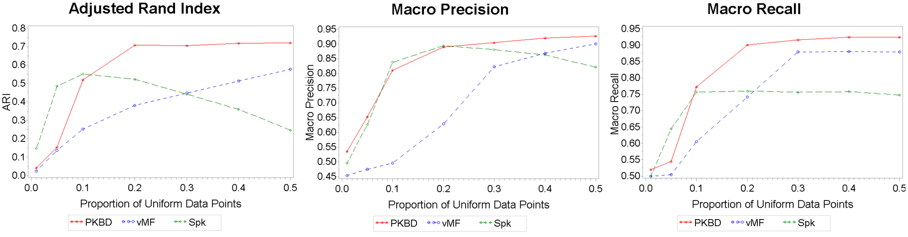
Figure 3: ARI, Macro-Precision, Macro-Recall of mix-PKBD, mix-vMF and Spkmeans algorithms. Data are generated from a mixture of a uniform distribution with proportions given in the $x$-axis and a PKBD ($\rho=0.9$) distribution. Sample size is 200 and the number of Monte Carlo replications is 100. Dimension $d=5$.

Effect of overlapping components: We define overlap of components by how close their centers are on the scale of the cosine of the angle created by the vector of the individual centroids. Specifically, we generated data first from a mixture of three component densities, one uniform and two PKBD ($\rho=0.9$), with sample size equal to $200$. The number of Monte Carlo replications is $100$. To be able to control the cosine of the angle between two centroid vectors, and therefore the component overlap, we consider the centroid vectors defined as $\mbox{\boldmath$\mu$}_{1}^{T}=(1,0,0),\mbox{\boldmath$\mu$}_{2}^{T}=(a,0,\sqrt{1-a^{2}})$. Then $\cos(\mbox{\boldmath$\mu$}_{1},\mbox{\boldmath$\mu$}_{2})=a$, and the value of cosine between the two centers can be controlled as the parameter $a$ varies.

Figure 4 plots the ARI, macro precision and macro recall as a function of the cosine between the two centroids. Here, we study the effect of overlap in the presence of noise. Figure 4 shows that the new method outperforms in terms of ARI and macro recall the mix-vMF and Spkmeans algorithms and it performs equivalently to mix-vMF in terms of macro precision when the cosine between the centroids is less than or equal to 0.3.

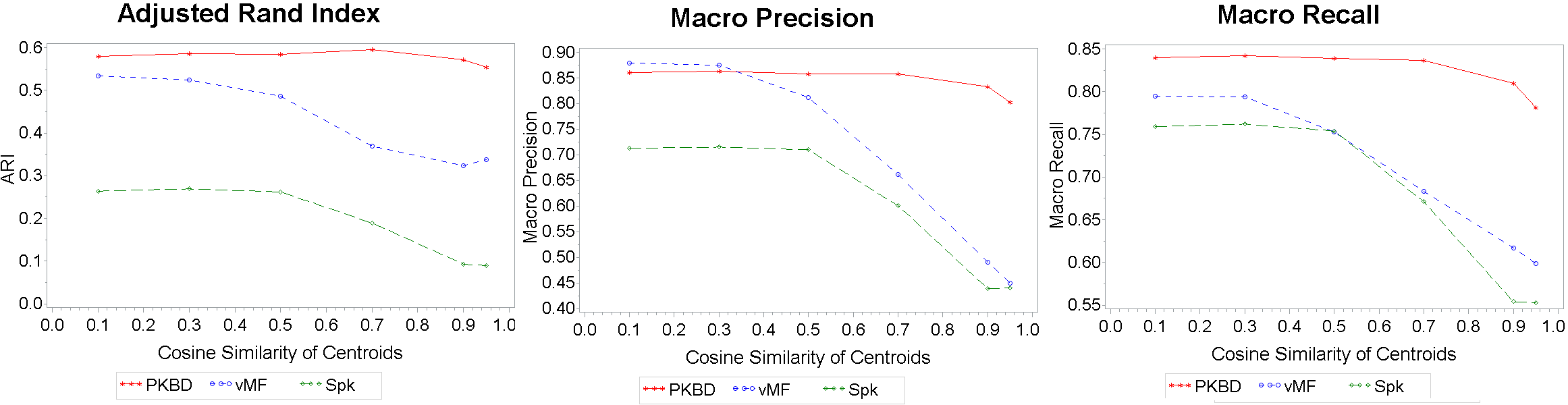
Figure 4: ARI, Macro-Precision, Macro-Recall of mix-PKBD, mix-vMF and Spkmeans algorithms. Data are generated from a mixture of one uniform (50%) and two equaly weighted PKBD ($\rho=0.9$) distributions with the cosine similarity of centroids given in the $x$-axis. Sample size is 200 and the number of Monte Carlo replications is 100. Dimension $d=3$.

We then generated data on the $3$-dimensional sphere from a mixture of three equally weighted PKBD ($\rho=0.9$), with sample size and the number of Monte Carlo replications as above. To be able to control the cosine of the angle between the centroid vectors, and therefore the component overlap, we consider the centroid vectors defined as $\mbox{\boldmath$\mu$}_{1}^{T}=(1/a,0,1),\mbox{\boldmath$\mu$}_{2}^{T}=(-1/2a,\sqrt{3}/2a,1),$ and $\mbox{\boldmath$\mu$}_{3}^{T}=(-1/2a,-\sqrt{3}/2a,1)$ after normalizing to length one. Then $\cos(\mbox{\boldmath$\mu$}_{i},\mbox{\boldmath$\mu$}_{j})=\frac{2a^{2}-1}{2(a^{2}+1)},i\neq j,i,j=1,2,3.$ Therefore, the value of the cosine between any two of the three centers can be controlled as the parameter $a$ varies.

Figure 5 plots the ARI, macro-precision and macro-recall of the three algorithms as a function of the cosine of the angle between any two centroid vectors. The graph indicates the following: a) when the cosine value is small, indicating a small amount of overlap between the different components, mix-PKBD and Spkmeans exhibit the highest values of macro-precision and recall. However, when the cosine of the angle is greater than or equal to $0.7$, mix-PKBD exhibits the best performance.

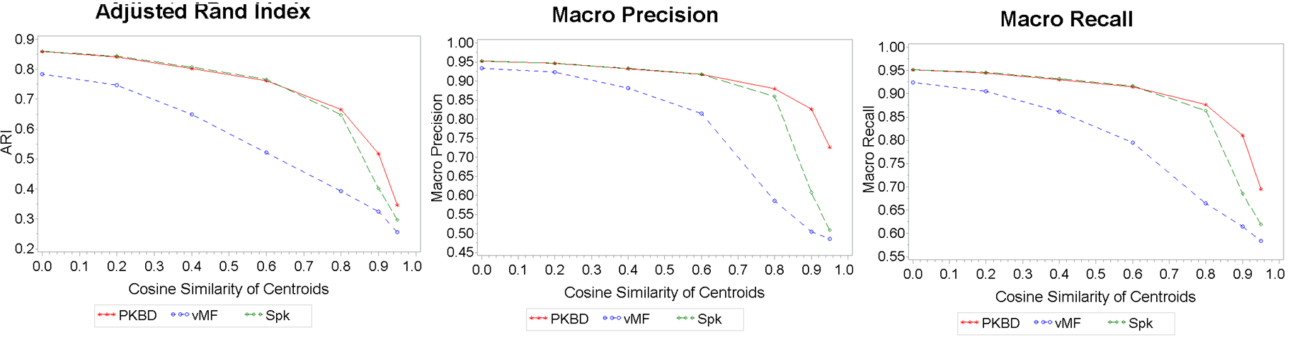
Figure 5: ARI, Macro-Precision, Macro-Recall of mix-PKBD, mix-vMF and Spkmeans algorithms. Data are generated from a mixture of three equaly weighted PKBD ($\rho=0.9$) distributions with the cosine similarity of centroids given in the $x$-axis. Sample size is 200 and the number of Monte Carlo replications is 100. Dimension $d=3$.

Tables A2 and A3 of the supplemental material present ARI, macro-precision and macro recall of the three algorithms under consideration when the sample size increases but the dimension stays fixed, and when the dimension increases but the sample size stays fixed. Data of equal proportions were generated from a mixture of uniform and either PKBD or vMF densities. Overall, when the sample size increases mix-PKBD seems to have the highest macro-precision, recall and ARI, after taking into account the standard error of the estimates of the performance measures. When the sample size is fixed but the dimension increases, mix-PKBD performs almost equivalently with mix-vMF algorithm, while Spkmeans indicates lesser performance than the other two algorithms.

Figures A4-A6 of the supplemental material investigate the effect of number of clusters, and also the effect of the value of the concentration parameter of the PKBD components on the performance of the mix-PKBD algorithm, while figure A7 shows that there is no significant difference in the run time between the different algorithms.

8.3 Application to Real Data

We now apply our method on well known data sets; detailed description of the data sets is provided in the on-line supplemental material. The data points are projected onto the sphere by normalizing them so the associated vectors have length one. The data sets were selected to exhibit different sample sizes, dimensions, and number of clusters. For the text data sets, we used Correlated Topic Modeling (CTM) (Blei and Lafferty, 2007; Grün and Hornik, 2017) for the dimension reduction and topics were used as features instead of words.

Table A4 of the supplemental material presents the results for all examples, that show, in most cases, mix-PKBD exhibits higher values of the evaluation indices than mix-vMF oe Spkmeans. To further illustrate the methods, we discuss here in some detail the Seeds and the Crabs data sets.

Seeds Data: We fitted a mix-PKBD$(\rho_{i})$ model to this data set. The empirical densities distance plot $(\beta=0.1)$ estimated the number of clusters to be 3 (see Figure A9 in Appendix A). The mixing proportions are $(0.2578,0.3302,0.4120)$ and the concentration parameters of the PKBD densities were 0.9922, 0.9866 and 0.9866, respectively. The inner products $\mbox{\boldmath$\mu$}_{1}.\mbox{\boldmath$\mu$}_{2}$ , $\mbox{\boldmath$\mu$}_{1}.\mbox{\boldmath$\mu$}_{3}$ and $\mbox{\boldmath$\mu$}_{2}.\mbox{\boldmath$\mu$}_{3}$ where $\mbox{\boldmath$\mu$}_{1},\mbox{\boldmath$\mu$}_{2},\mbox{\boldmath$\mu$}_{3}$ are the cluster centroids are 0.9839, 0.9974 and 0.9916 indicating that the three clusters have a fair amount of overlap. Figure A10 indicates graphically the overlap among the different clusters.

Crabs Data: The second data set is the crabs data, details of which are presented in the supplemental material (Section C of Appendix A). For this data set we first run mix-PKBD with the number of clusters equal to 2. We also run mix-vMF and Spkmeans again using two clusters with the two color species indicating the classes. In this case, the performance of mix-VMF and Spkmeans was surprisingly poor. To assess cluster homogeneity we present Figures A11 and A12 (supplemental material), and the scatter plot matrices for this data set by species (blue or green crabs) and by sex, respectively. Each clustering algorithm discovers structure in the data; the mix-PKBD model seems to cluster the data according to species where the degree of separation is higher than clustering according to sex. The clusters produced by mix-vMF and Spkmeans are more likely to correspond to clustering by gender and not species.

We also computed the empirical densities distance plot (see Figure A13 of the supplemental material). This plot estimates the number of clusters as four and it seems that clusters are formed by species and gender. We also run mix-vMF and Spkmeans models with four clusters. Table S6 of the supplemental material, Appendix B presents the performance measures for all models, indicating that all perform equivalently.

9 Discussion & Conclusion

We introduced and discussed a novel model for clustering directional data that is based on the Poisson kernel. We presented connection of the Poisson kernel based density function with other models that are used for the analysis of directional data. We developed a clustering algorithm that is based on a mixture of PKBD, studied the identifiability of the proposed model, the convergence of the associated algorithm and, via simulation and application to real data, we compared the performance of the proposed clustering algorithm with the algorithm proposed by Banerjee et al. (2005) and Spkmeans. Furthermore, we investigated practical issues associated with the operationalization of our procedure, and proposed a natural method to estimate the number of clusters from the data.

Our methods are based on mixtures of PKBD and as such are model based. McNicholas (2016) argues in favor for model based clustering methods. Our results indicate that our methods, in all cases examined, exhibit excellent performance when compared with state of the art methods.

An interesting aspect of clustering based on the mix-PKBD model is the robustness exhibited in the presence of noise. Our model exhibits the best performance in terms of macro-precision and recall especially when the proportion of noise is high. On the other hand, mix-PKBD performs similarly with the other two methods when the amount of noise is low. There are cases where mix-PKBD has inferior performance than mix-vMF and Spkmeans in terms of macro-precision and recall. We generated data from a mixture of vMF($\kappa=40$) and a PKBD($\rho=0.8$) distributions. The cosine between the center vectors of the components was 0.75 indicating an approximately $41\circ$ angle. When the mixing propor tion of the PKBD(0.8) was greater than 0.6, mix-PKBD exhibited higher macro-precision & recall than mix-vMF and Spkmeans (data are not shown). Note that PKBD(0.8) was selected so that the mode of vMF and PKBD(0.8) distributions are approximately the same. The dimension of the data in this case equals three.

Poisson kernel-based mixture models offer a natural way to estimate the number of clusters. We introduced the empirical densities distance plot that can be used to estimate 25 the number of clusters when the data are clustered using mix-PKBD. We note here that the empirical densities distance plot depends on a tuning parameter $\beta$. When the clustering model is a mixture of PKBD with a common $\rho$, we conjecture that $\beta$ can be selected such that $\beta\leq\hat{\rho}$, where $\hat{\rho}$ is an estimate of $\rho$. When the clustering model is a mixture of PKBD with different parameters ρi, we conjecture that $\beta\leq\min\limits_{i}\{\hat{\rho}_{i}:1\leq i\leq M\}$. Additional work is needed to fully understand the selection of the tuning parameter β and the performance of the distance plot.

SUPPLEMENTAL MATERIALS

Title:

Appendix A ”Poisson Kernel-Based Clustering on the Sphere: Convergence Properties, Identifiability, and a Method of Sampling”
Appendix A is organized in four sections. Section A presents detailed proofs of the propositions that appear in this manuscript. Section B presents calculations and simulations associated with the estimation of the number of clusters. Section C includes additional simulation examples and application of our methods in a variety of data sets, while Section D offers additional tables and graphs illustrating further comparison of the PKBD model with the von Mises-Fisher model, and the elliptically symmetric angular Gaussian (ESAG) model.

Title:

Appendix B; Codes Associated with ”Poisson Kernel-Based Clustering on the Sphere: Convergence Properties, Identifiability, and a Method of Sampling”

References

- Axler et al. (2001) Axler, S., Bourdon, P., and W. Ramey, W. (2001), Harmonic Function Theory, (2nd edition), Springer-Verlag, New York.
- Banerjee et al. (2003) Banerjee, A., Dhillon, I. S., Ghosh J., and Sra, S. (2003), ”Generative Model-based Clustering of Directional Data,” In ACM SIGKDD International Conference on Knowledge Discovery and Data Mining (KDD), 19-29
- Banerjee et al. (2005) —– (2005), ”Clustering on the Unit Hypersphere using von Mises-Fisher Distributions,” Journal of Machine Learning Research, 6, 1345-1382.
- Banerjee and Ghosh (2002) Banerjee, A. and Ghosh J. (2002), ”Frequency Sensitive Competitive Learning for Clustering on High-dimensional Hyperspheres,” In Proceedings International Joint Conference on Neural Metworks 1590-1595.
- Banfield and Raftery (1993) Banfield, J. D. and Raftery, E. (1993), ”Model-Based Gaussian and Non-Gaussian Clustering,” Biometrics 49(3), 803-821.
- Bijral et al. (2007) Bijral, A. S., Breitenbach, M., and Grudic, G. (2007), ”Mixture of Watson Distributions: A Generative Model for Hyperspherical Embeddings,” In: Artificial Intelligence and Statistics AISTATS 35-42.
- Bilmes (1997) Bilmes, J. A. (1997), ”A Gentle Tutorial on the EM Algorithm and its Application to Parameter Estimation for Gaussian Mixture and Hidden Markov Models,” Technical Report ICSI-TR-97-021, University of California, Berkeley.
- Blei et al. (2003) Blei, D. M, Ng, A. Y. and Jordan, M. I. (2003) ”Latent Dirichlet Allocation,” Journal of Machine Learning Research, 3, 993-1022.
- Blei and Lafferty (2007) Blei, D. M, Lafferty, J. D. (2007) ”A Correlated Topic Model of Science,” The Annals of Applied Statistics, 1(1), 17-35.
- Dai and Xu (2013) Dai, F., and Xu, Y. (2013), Approximation Theory and Harmonic Analysis on Sphere and Balls, Springer-Verlag, New York.
- Dempster et al. (1977) Dempster, A. P., Laird, N. M., and Rubin, D. B. (1977), ”Maximum Likelihood from Incomplete Data via the EM Algorithm,” Journal of the Royal Statistical Society, Series B, 39(1), 1-38.
- Dhillon and Modha (2001) Dhillon, I. S., and Modha, D. S. (2001), ”Concept Decompositions for Large Sparse Text Data using Clustering,” Machine Learning, 42(1), 143-175.