Event-based Moving Object Detection and Tracking

Abstract

Event-based vision sensors, such as the Dynamic Vision Sensor (DVS), are ideally suited for real-time motion analysis. The unique properties encompassed in the readings of such sensors provide high temporal resolution, superior sensitivity to light and low latency. These properties provide the grounds to estimate motion efficiently and reliably in the most sophisticated scenarios, but these advantages come at a price - modern event-based vision sensors have extremely low resolution, produce a lot of noise and require the development of novel algorithms to handle the asynchronous event stream.

This paper presents a new, efficient approach to object tracking with asynchronous cameras. We present a novel event stream representation which enables us to utilize information about the dynamic (temporal) component of the event stream. The 3D geometry of the event stream is approximated with a parametric model to motion-compensate for the camera (without feature tracking or explicit optical flow computation), and then moving objects that don’t conform to the model are detected in an iterative process. We demonstrate our framework on the task of independent motion detection and tracking, where we use the temporal model inconsistencies to locate differently moving objects in challenging situations of very fast motion.

Supplementary material

The supplementary video materials and datasets will be made available at http://prg.cs.umd.edu/BetterFlow.html

The C++ implementation of the Algorithms 1 and 2 can be found here: https://github.com/better-flow/better-flow. We provide experimental Python bindings here: https://github.com/better-flow/pydvs

I Introduction and Philosophy

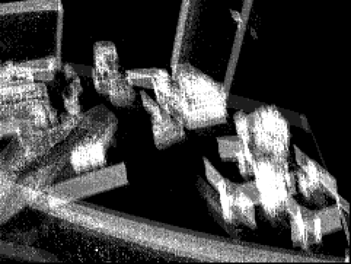
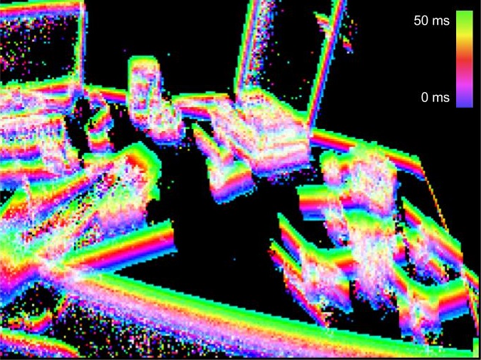
(a)	(b)
(c)	(d)

Figure 1: Illustration of parametric model-fitting by alignment. The input is a cloud of events within a small time interval $\delta t$. Visualization of event counts (a), and average time stamps (b) mapped to the image pixels after reprojection. Motion-compensated event count (c) and time image (d) acquired after the minimization stage. Colors encode the event time stamp value (with blue for oldest and green for the most recent events). Note the hand that moves independently from the camera is clearly visible on the time image, which is the basis for the subsequent detection and tracking.

The recent advancements in imaging sensor development have outpaced the development of algorithms for processing image data. Recently, the computer vision community has started to derive inspiration from the neuromorphic community whose ideas are based on biological systems to build robust and fast algorithms which run on limited computing power. These algorithms are more pervasive than ever before due to the advent of smart phones and smart cameras for a wide variety of uses from security, tracking, pursuit and mapping.

The human fascination to understand ultra-efficient flying beings like bees, birds and flies has led the pioneers of the field [10] to conceptualize the usage of optical flow as the ultimate representation for visual motion. The availability of optical flow makes a large variety of the aforementioned tasks simple applications of the analysis of the flow field. The computation of this superlative representation is often expensive, hence the computer vision community has come up with alternative formulations for high speed robust optical flow computation under certain constraints.

At the same time, the robotics community follows the approach of building 3D models for their wide spread applicability in planning algorithms and obstacle avoidance. One could accomplish any real-world task with a full 3D reconstruction of the scene from a traditional camera or other sensors. However, bio-organisms do not “see” the world in-terms of frames – which is a redundant but convenient representation used by most robotics and computer vision literature. They “see” the world in-terms of asynchronous changes in the scene [19, 24]. This gives unparalleled advantage in-terms of temporal resolution, low latency, and low bandwidth motion signals, potentially opening new avenues for exciting research and applications. The availability of sensors which capture events has attracted the research community at large and is gaining momentum at a rapid pace.

Most challenging problems are encountered during scenarios requiring the processing of very fast motion with real-time control of a system. One such scenario is encountered in autonomous navigation. Although computer vision and robotics communities have put forward a solid mathematical framework and have developed many practical solutions, these solutions are currently not sufficient to deal with scenes with very high speed motion, high dynamic range, and changing lighting conditions. These are the scenarios where the event based frameworks excel.

Based on the philosophy of active and purposive perception, in this paper, we focus on the problem of multiple independently moving object segmentation and tracking from a moving event camera. However, a system to detect and track moving objects requires robust estimates of its own motion formally known as the ego-motion estimation. We use the purposive formulation of the ego-motion estimation problem – image stabilization. Because, we do not utilize images, we formulate a new time-image representation on which the stabilization is performed. Instead of locally computing image motion at every event, we globally obtain an estimate of the system’s ego-motion directly from the event stream, and detect and track objects based on the inconsistencies in the motion field. This global model achieves high fidelity and performs well with low-contrast edges. The framework presented in the paper is highly parallelizable and can be easily ported to a GPU or an FPGA for even lower latency operation.

The contributions of this paper are:

• A novel event-only feature-less motion compensation pipeline.

• A new time-image representation based on event timestamps. This representation helps improve the robustness of the motion compensation.

• A new publicly available event dataset (Extreme Event Dataset or EED) with multiple moving objects in challenging conditions (low lighting conditions and extreme light variation including flashing strobe lights).

• A thorough quantitative and qualitative evaluation of the pipeline on the aforementioned dataset.

• An efficient C++ implementation of the pipeline which will be released under an open-source license.

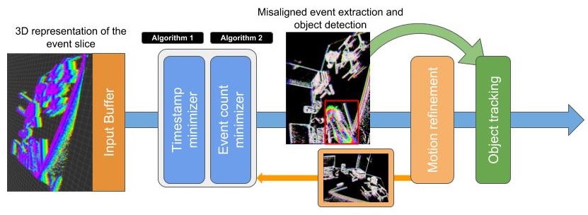
Figure 2: Motion compensation and independent object tracking pipeline. The event cloud motion is minimized with the error functions defined on the time-image $\mathcal{T}$ and then, the motion is refined by maximizing the event density on the event-count image $\mathcal{I}$. The subsets of events with high probability of misalignment (shown in red bounding box) are removed and tracked and the remaining event cloud is again motion-compensated.

II Related Work

Over the years, several researchers have considered the problem of event-based clustering and tracking. Litzenberger et al. [16] implemented, on an embedded system a tracking of clusters following circular event regions. Pikatkowska et al. [18] used a Gaussian mixture model approach to track the motion of people. Linares et al. [15] proposed an FPGA solution for noise removal and object tracking, with clusters initialized by predefined positions. Mishra et al. [17] assigned events to “spike groups”, which are clusters of events in space-time, Lagorce et al. [14] computed different features and grouped them for object tracking, and Barranco et al. [4] demonstrated a real-time mean-shift clustering algorithm.

A number of works have developed event-based feature trackers (e.g. [26]) and optical flow estimators ([2, 3]). Based on either tracking events or features, a number of visual odometry and SLAM (simultaneous localization and mapping) approaches have been proposed. First, simplified 3D motion and scene models were considered. For example, Censi et al. [6] used a known map of markers, Gallego et al. [7] considered known sets of poses and depth maps, and Kim et al. and Reinbacher et al. [12, 20] only considered rotation. Other approaches fused events with IMU data [26]. The first event-based solution for unrestricted 3D motion was presented by Kim et al. [13]. Finally, a SLAM approach that combines events with images and IMU for high speed motion was recently introduced by Vidal et al. in [23].

Most closely related to our work are two studies: the work by Gallego et al. [9] proposes a global 3D motion estimation approach for 3D rotation, and in [8] extensions of the approach are discussed. Recently in [21] a linear model for iterative segmentation was proposed. Vasco et al. [22] study the problem of independent motion detection in a manipulation task. The expected flow field in a static scene for a given motion is learned, and then independently moving objects are obtained by tracking corners and checking for inconsistency with the expected motion. In effect, the processes of 3D motion estimation and segmentation are separated. Here, instead we consider the full problem for a system with no knowledge about its motion or the scene. So far, no other existing event-based approach can detect moving objects in challenging situations.

III Method

Our algorithm derives inspiration from 3D point cloud processing techniques, such as Kinect Fusion [11], which use warp fields to perform a global minimization on point clouds. The algorithm performs global motion compensation of the camera by fitting a 4-parameter motion model to the cloud of events in a small time interval. These four parameters are the the x-shift, y- shift, expansion, and 2D rotation denoted as $(h_{x},h_{y},h_{z},\theta)$. We use two different error functions in the minimization in different stages of the algorithm, which are defined in equations 4 and 6. It can be shown that the 4-parameter model is a good approximation for rigid camera motion and fronto-parallel planar scene regions. The algorithm then looks for the event clusters which do not conform to the motion model and labels them as separately moving regions, while at the same time fitting the motion model to each of the detected regions.

Sec. IV-A describes the general notation used in this paper, and Secs. IV-B and IV-C provide an intuition for the error functions used for motion compensation. The details of the algorithm are described in Sec. V (motion compensation) and VI (object detection and tracking).

IV Preliminaries

IV-A Notation

Let the input events in a temporal segment $[t_{0},t_{0}+\delta t]$ be represented by a 3-tuple $C\{x,y,t\}\in\mathbb{R}^{3}$. Here $\left\{x,y\right\}$ denote the spatial coordinates in the image plane and $t$ denotes the event timestamps. $t_{0}$ can be arbitrarily chosen, as the DVS data is continuous. However, the algorithm functions on a small time segment $\delta t$.

Let us denote the 2D displacement that maps events $(x,y)$ at time $t$ to their locations $(x^{\prime},y^{\prime})$ at time $t_{0}$ by a warp field $\phi(x,y,t-t_{0}):(x,y,t)\xrightarrow{}(x^{\prime},y^{\prime},t)$. Our goal is to find the motion compensating warp field $\phi:\mathbb{R}^{3}\to\mathbb{R}^{3}$ such that the motion compensated events, when projected onto the image plane, have maximum density. Let us denote these motion compensated events as:

$$C^{\prime}=\Pi\{\phi(C)\}=\Pi\{\phi(x,y,t-t_{0})\}$$ (1)

$$=\{x^{\prime},y^{\prime},0\}\,\quad\forall\{x,y,t\}\in C$$

Due to the geometric properties of the events, such a warp field encodes the per-event optical flow. Here $\Pi$ is the temporal projection function projecting motion compensated events along the time axis. $\Pi$ is used to reduce the dimensionality of the data from $\mathbb{R}^{3}\to\mathbb{R}^{2}$ and simplify the minimization process. We represent the data available in $C$ with two discretized maps which encode the temporal and intensity properties of the event stream.

IV-B Event Count Image

To calculate the event density $\mathcal{D}$ of $C^{\prime}=\Pi\{\phi(C)\}$, we discretize the image plane into pixels of a chosen size. We use symbols $(i,j)\in\mathbb{N}^{2}$ to denote the integer pixel (discretization bin) coordinates, while $(x^{\prime},y^{\prime},t)\in\mathbb{R}^{3}$ represent real-valued warped event coordinates. Each projected event from $C^{\prime}$ is mapped to a certain discrete pixel, and the total number of events mapped to the pixel is recorded as a value of that pixel. We will henceforth refer to this data structure as event-count image $\mathcal{I}$. Let

$$\xi_{ij}=\{\{x^{\prime},y^{\prime},t\}:\{x^{\prime},y^{\prime},0\}\in C^{\prime},\,i=x^{\prime},\,j=y^{\prime}\}$$ (2)

be the proposed event trajectory - a set of warped events along the temporal axis which get projected onto the pixel $(i,j)$ after the $\phi$ operation has been applied. Then the event-count image pixel $\mathcal{I}_{ij}$ is defined as:

$$\mathcal{I}_{ij}=|\xi_{ij}|$$ (3)

Here, $|A|$ is the cardinality of the set $A$. The event density $\mathcal{D}$ is computed as:

$$\mathcal{D}=\frac{\sum_{i,j}\mathcal{I}_{ij}}{\#\mathcal{I}}=\frac{|C^{\prime}|}{\#\mathcal{I}}$$ (4)

where, $\#\mathcal{I}$ denotes the number of pixels with at least one event mapped on it. Since $|C^{\prime}|$ is a constant for a given time slice, the problem can be reformulated as the minimization of the total area $S=\#\mathcal{I}$ on the event-count image. A similar formulation was used in [9] to estimate the rotation of the camera with the acutance as an error metric, instead of the area.

IV-C Time-image $\mathcal{T}$

Keen readers would observe that the event-count image representation $\mathcal{I}$ suffers from a subtle drawback. When the projection operation is performed, events produced by different edges (edges corresponding to different parts of the same real-world object or different real-world objects) can get projected onto the same pixel. This is a very common situation which occurs during fast motion in highly textured scenes.

To alleviate this problem, we utilize the information from the event timestamps $t$ by proposing a novel representation which we call the time-image $\mathcal{T}$. Similar to $\mathcal{I}$ described before, $\mathcal{T}$ is a discretized plane with each pixel containing the average timestamp of the events mapped to it by the warp field $\phi$.

$$\mathcal{T}_{ij}=\frac{1}{\mathcal{I}_{ij}}\sum t:t\in\xi_{ij}$$ (5)

Computing the mean of timestamps allows us to increase fidelity of our results by making use of all available DVS events. An alternative approach would be to consider only the latest timestamps [25], where performance would suffer in low light situations. This is because the signal to noise ratio in DVS events depends on the average illumination, the smaller the average illumination, the larger the noise. Note that the value of a time-image pixel ${\mathcal{T}}_{ij}$ (or better its deviation from the mean value) correlates with the probability that the motion was not compensated locally - this will be used later for motion detection in Sec. VI-A. $\mathcal{T}$ follows the 3D structure of the event cloud, and its gradient $(G)$ provides the global metrics of the motion-compensation error which will be minimized by the algorithm:

$$Error=\sum\left\lVert G[i,j]\right\rVert=\sum(G_{x}^{2}[i,j]+G_{y}^{2}[i,j])$$ (6)

Here $(G_{x}[i,j],G_{y}[i,j])$ denote the local spatial gradient of $\mathcal{T}$ along the $(x)$ or $(y)$ axes. Equation 6 is a global error which takes into account local motion inconsistencies of the warped event cloud. Together with the rigid body motion assumption, equation 6 can be decomposed into equations:

$$d_{x}=\frac{\sum G_{x}[i,j]}{\#\mathcal{I}},\qquad d_{y}=\frac{\sum G_{y}[i,j]}{\#\mathcal{I}}$$ (7)

$$d_{z}=\frac{\sum(G_{x}[i,j],G_{y}[i,j])\cdot(i,j)}{\#\mathcal{I}}$$ (8)

$$d_{\theta}=\frac{\sum(G_{x}[i,j],G_{y}[i,j])\times(i,j)}{\#\mathcal{I}}$$ (9)

Equations 7, 8 and 9 will be used to provide gradients for the motion compensation algorithm in Sec. IV-D - each of them correspond to the error for one of the model parameters: $(h_{x},h_{y},h_{z},h_{\theta})$, which represent shift in the image plane, expansion and 2D rotation.

IV-D Minimization Constraints

The local gradients of $\mathcal{T}$ and the event density $\mathcal{D}$ both quantify the error in event cloud motion compensation. We model the global warp field $\phi^{G}(x,y,t)$ with a 4 parameter global motion model $\mathcal{M}^{G}=\{h_{x},h_{y},h_{z},\theta\}$ to describe the distortion induced in the event cloud by the camera motion. The resulting coordinate transformation amounts to:

Here the the original event coordinates $\left\{x,y,t\right\}$ are transformed into new coordinates $\left\{x^{\prime},y^{\prime},t\right\}$. Note that the timestamp remains unchanged in the transformation and is omitted in Eq. 10 for simplicity. Furthermore, we assume linear event trajectories $\xi_{ij}$ (Eq. 2) within the time slice.

The parameters of the model denote the shift $(h_{x},h_{y})$ parallel to the image plane, a motion (h_z) towards the image plane, effectively a radial expansion of the event cloud, and a rotation $(\theta)$ around the $Z$ axis, effectively a circular component of the event cloud.

V Camera Motion Compensation

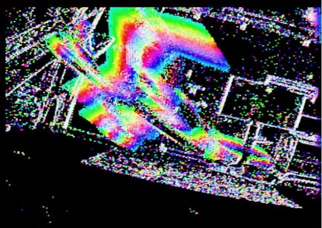
Figure 3: An example output of the motion compensating algorithm - the time-image. The colors denote the average timestamps (blue is $t_{0}$, green is $t_{0}+\delta t$). On this example the separately moving object (drone) occupies the large area of the frame but the camera motion compensation still succeeds.

Our pipeline (see Fig. 2) consists of camera motion compensation and subsequent motion inconsistency analysis to detect independently moving objects. To compensate for the global background motion, the four parameter model $\mathcal{M}^{G}$ presented in Sec. IV-D is used. The background motion is estimated, and objects are detected. Then the background model is refined using data from the background region only (not the detected objects) (Fig. 3), and four-parameter models are fit to the segmented objects for tracking.

As outlined in Secs. IV-B and IV-D, $\mathcal{T}$ and $\mathcal{I}$ are local metrics of event cloud misalignment but based on different sources of data - event timestamps and event rates. $\mathcal{T}$ provides a poor error metric when the optimizer is close to the minima due to the event averaging scheme employed. In particular, the global error gradient functions (Eqs. 7 - 9) have very small values and are unreliable.

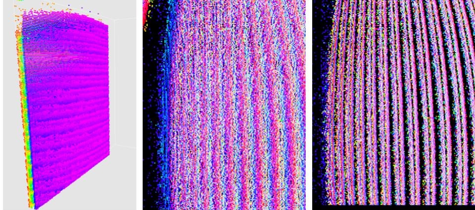
Figure 6: An experiment with high texture and fast motion. The event cloud is a set of tilted planes which overlap during vertical projection. The time-image is a robust enough metric to compute the correct minimization gradient for the motion compensation. Images from left to right: 3D representation of event cloud, unminimized time-image, minimized time-image.

Note that, $\mathcal{T}$ provides reliable gradients of the parameters of model $\mathcal{M}^{G}$ even in the presence of noise and fast motion, when events from different edges overlap during projection (see Fig. 6).

For the aforementioned reasons, the global motion minimization is performed in two stages: coarse motion minimization on $\mathcal{T}$ and fine motion refinement on the $\mathcal{I}$.

Data: $\mathcal{M}_{i-1}^{G},C,d,\xi$

Result: $\mathcal{M}_{i}^{G},C^{\prime},\mathcal{T}$

Algorithm 1 Global motion compensation in event space using $\mathcal{T}$.

V-A Coarse Global Motion Minimization on $\mathcal{T}$

An algorithm for coarse motion compensation of the event cloud is presented in Algorithm 1.

The input is the previous model $\mathcal{M}_{i-1}^{G}$, original event cloud $C$, the discretization grid size $d$ and accuracy parameter $\xi$. The warpEventCloud function applies the warp field $\psi$ as per equation (10). The time-image $\mathcal{T}$ is then generated on the warped event cloud $C^{\prime}$ according to (5). Finally, updateModel computes gradient images $G_{x}$ and $G_{y}$ (a simple Sobel operator is applied) and the gradients for the motion model parameters $\mathcal{M}_{i}^{G}$ are computed with (7 - 9). The parameters of $\mathcal{M}_{i}^{G}$ are then updated in a gradient descent fashion. In this paper, the discretization parameter $d$ has been chosen as $0.3$ of the DVS pixel size.

V-B Fine Global Motion Refinement on $\mathcal{I}$

An additional fine motion refinement is done by maximizing the density $\mathcal{D}$ (4) of the event-count image $\mathcal{I}$. The density $\mathcal{D}$ function does not explicitly provide the gradient values for a given model, so variations of model parameters are used to acquire the derivatives and perform minimization. The corresponding algorithm is given in Algorithm LABEL:alg:ec.

Data: $\mathcal{M}_{i-1}^{G},C,d,\xi$

Result: $\mathcal{M}_{i}^{G},C^{\prime},\mathcal{I}$

Algorithm 2 Global motion compensation in event space with event count image

VI Multiple Object Detection And Tracking

Figure 4: A frame from the ’Two Objects’ dataset. The left image shows the misalignment of the two objects after the global motion compensation (green color corresponds to the most recent events). The right image is the corresponding grayscale image - the objects (highlighted by bounding boxes) are poorly visible due to severe motion blur.

In this section, we describe the approach of the detection of independently moving objects by observing the inconsistencies of $\mathcal{T}$. The detected objects are then tracked using a traditional Kalman Filter.

VI-A Detection

We use a simple detection scheme: We detect pixels as independently moving using a thresholding operation and then group pixels into objects using morphological operations. Each pixel $\left\{i,j\right\}\in\mathcal{T}$ is associated with a score $\rho(x_{i},y_{j})\in[-1,1]$ defined in Eq. 11, which quantitatively denotes the misalignment of independently moving objects with respect to the background. $\rho$ is used as a measure for classifying a pixel as either background $\mathcal{B}$ or independently moving objects $\mathcal{O}_{k}$.

$$\rho(i,j)=\frac{\mathcal{T}(i,j)-{<\mathcal{T}_{i,j}>}}{\triangle t}$$ (11)

with $<>$ denoting the mean. Now, let us define $\mathcal{B}$ and $\mathcal{O}_{k}$.

$$\mathcal{B}=\{(i,j)|\rho(i,j)\leq 0\}\qquad\mathcal{O}=\{(i,j)|\rho(i,j)>\lambda\}$$ (12)

here $\mathcal{O}=\mathcal{O}_{1}\bigcup...\mathcal{O}_{n}$ ($n$ is the number of independently moving objects) and $\lambda$ is a predefined minimum confidence values for objects to be classified as independently moving. To detect independently moving objects, we then group foreground pixels using simple morphological operations.

VI-B Tracking

The detection algorithm presented in Subsec. VI-A runs in real-time (processing time $<\delta t$) and is quite robust. To account for missing and wrong detections, especially in the presence of occlusion, we employ a simple Kalman Filter with a constant acceleration model. For the sake of brevity, we only define the state ($\mathcal{X}_{k}$) and measurement vectors ($\mathcal{Z}_{k}$) for the $k^{\text{th}}$ object.

$$\begin{array}[]{lcl}\mathcal{X}_{k}=[\hat{x}_{k},\hat{y}_{k},h_{x},h_{y},h_{z},\theta,\hat{u}_{k},\hat{v}_{k}]^{T}\end{array}$$ (13)

$$\begin{array}[]{lcl}\mathcal{Z}_{k}=[\hat{x}_{k},\hat{y}_{k},h_{x},h_{y},h_{z},\theta]^{T}\end{array}$$ (14)

where $\left\{\hat{x}_{k},\hat{y}_{k}\right\}$ represent the mean coordinates of $\mathcal{O}_{k}$, $h_{x},h_{y},h_{z},\theta$ represent the model parameters of the object, which is obtained by motion-compensating $\mathcal{O}_{k}$ as described in V and $\hat{u}_{k},\hat{v}_{k}$ represents the average velocity of the $k^{\text{th}}$ object.

VII Datasets and Evaluation

The Extreme Event Dataset (EED) used in this paper was collected using the DAVIS [5] sensor under two scenarios. First, it was mounted on a quadrotor (Fig. 7), and second in a hand-held setup to accommodate for a variety of non-rigid camera motions. The recordings feature objects of multiple sizes moving at different speeds in a variety of lighting conditions. We emphasize the ability of our pipeline to perform detection at very high rates, and include several sequences where the tracked object changes its speed abruptly.

Figure 5: An example from the strobe dataset. A single object moves in a dark room with a bright strobe light which produces a lot of noise on the sensor output. Since the motion model is global, the minimization and detection are tolerant to such noise. The detection output is shown with a superimposed bounding box.

We have collected over 30 recordings in total but the centerpiece of our dataset is the ’Strobe Light’ sequence. In this sequence, a periodically flashing bright light in a dark room creates significant noise. At the same time an object, another quadrotor is moving in the room. This is a challenge for traditional visual systems, but our bio-inspired algorithm shows excellent performance by leveraging the high temporal event density of the DAVIS sensor.

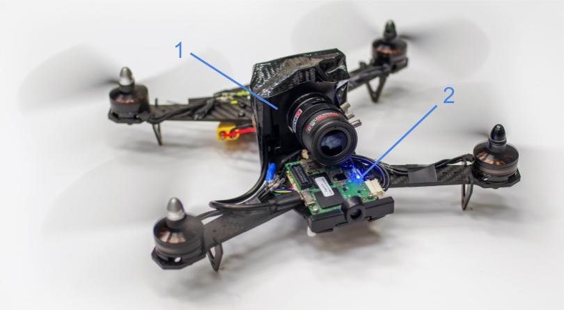
Figure 7: Drone used in the dataset collection. 1 - mounted DAVIS240B camera, 2 - Customized Qualcomm Flight platform with onboard computer

VII-A Dataset collection

The dataset was collected using the DAVIS240B bio-inspired sensor equipped with a $3.3mm.$ lens with a horizontal and vertical field of view of $80^{\circ}$. Most of the sequences were created in a hand-held setting. For the quadropter sequences, we modified a Qualcomm Flight${}^{\text{TM}}$ [1] platform to connect the DAVIS240B sensor to the onboard computer and collect data in a realistic scenario.

The setup of the quadrotor+sensor platform can be seen in Fig. 7. The overall weight of the fully loaded platform is $\approx 500g.$ and it is equipped with the Snapdragon APQ8074 ARM CPU, featuring 4 cores with up to 2.3GHz frequencies.

VII-B Computation Times

On a single thread of Intel Core${}^{\text{TM}}$ i7 3.2GHz processor, Algorithms 1 and LABEL:alg:ec take $10ms$ and $7ms$ on average for a single iteration step. However, both algorithms are based on a warp-and-project $\Pi\{\phi(C)\}$ operation which is highly parallelizable and thus well fit for implementation on a Graphical Processing Unit (GPU) or a Field-Programmable Gate Array (FPGA) to acquire very low latency and high processing speeds.

While a low level hardware implementation is beyond the scope of this paper, we tested a prototype of the algorithm on an NVIDIA Titan X Pascal${}^{\text{TM}}$ GPU with CUDA acceleration. A single iteration for Algorithms 1 and LABEL:alg:ec takes $0.01ms$ and $0.003ms$ on average, respectively, which is a 1000X and 2333X speed-up. We have empirically found that the minimization converges on average in less than 30 iterations which ensures a faster-than-real-time computation speed with a high margin.

The recordings are organized into several sequences according to the nature of scenarios present in the scenes. All recording feature a variety of camera motions, with both rotational and translational motion (See fig. 9):

• ”Fast Moving Drone” - A sequence featuring a single small remotely controlled quadrotor. Quadrotor has a rich texture and moves across various backgrounds in daylight lighting conditions following a variety of trajectories.

• ”Multiple objects ” - This sequence consists of multiple recordings with 1 to 3 moving objects under normal lighting conditions. The objects are simple, some of them have little to no texture. The objects move at a variety of speeds, either along linear trajectories or they bump from a surface.

• ”Lighting variation” - A strobe light flashing at frequencies of 1-2 Hz was placed in a dark room to produce a lot of noise in the event sensor. This is an extremely challenging sequence, otherwise similar to the ”Fast Moving Drone”.

• ”What is a Background?” - In most tracking algorithm evaluations, object moves in front of the background. The following toy sequence was included, to show that it is possible to track an object even when the background occupies the space in between the camera and the object: A simple object was placed behind the net and the motion could only be seen through the net. Recordings contain a variety of distances between the net and the camera and the object is thrown at different speeds.

• ”Occluded Sequence” - The sole purpose of this sequence is to test the reliability of tracking in scenarios when detection is not possible for a small period of time. Several recordings feature object motion in occluded scenes.

VII-C Metrics and Evaluation

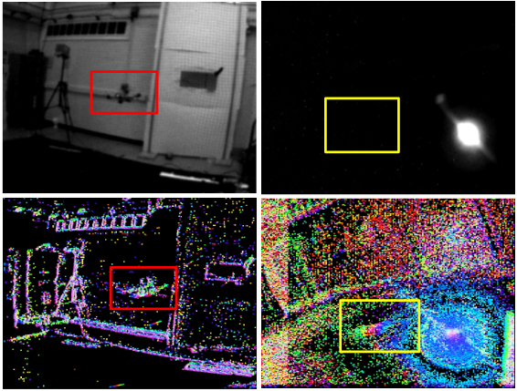
Figure 8: Common failure cases. Top row: RGB frames, bottom row: time-images. Left: A setting featuring an object which does not move with respect to the background - a failure case for the detection stage, even though the edges are visible. Right: High noise scenario with the tracked object not visible in the gray-scale image.

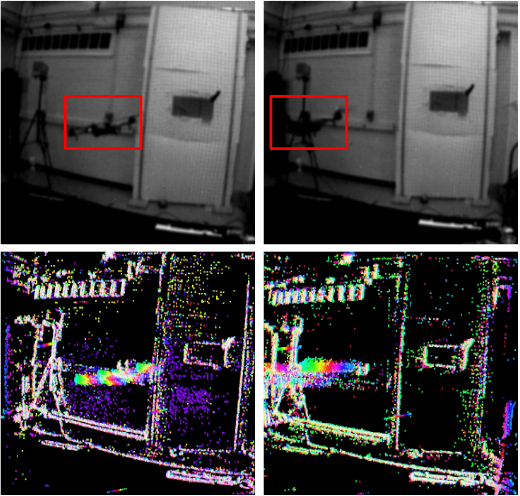
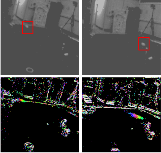
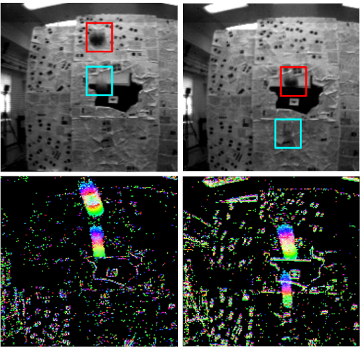
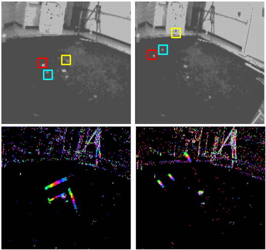
(a)	(b)	(c)	(d)
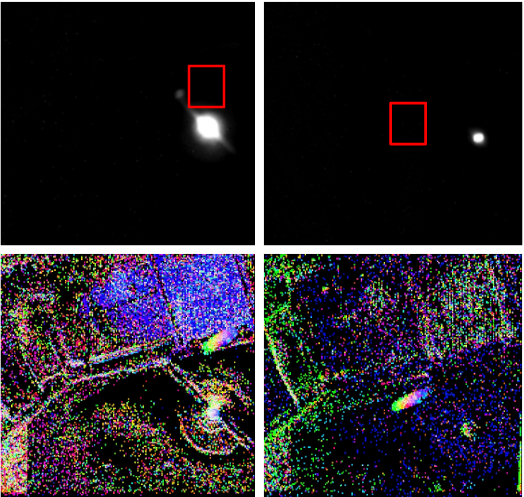
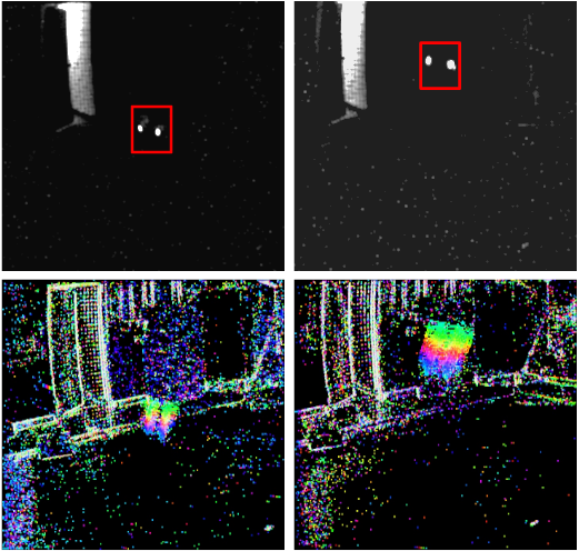
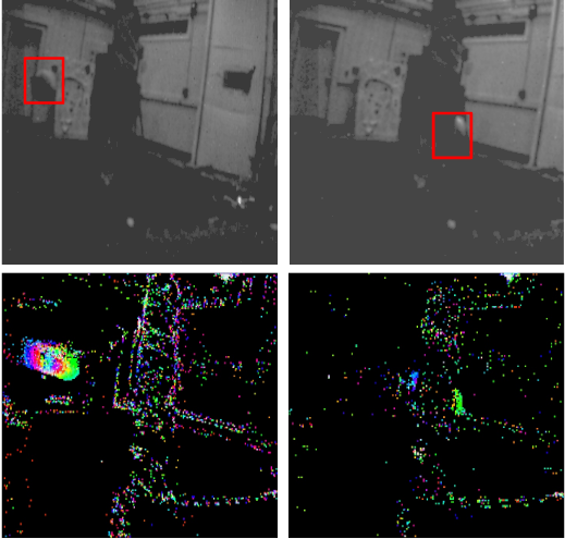
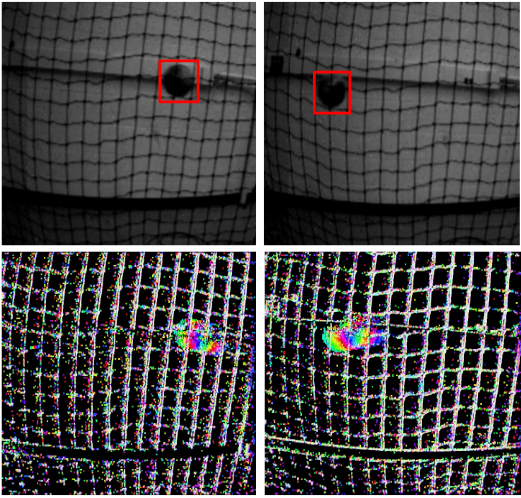
(e)	(f)	(g)	(h)

Figure 9: Sample frames from the EED dataset are shown. Top row shows RGB frames with superimposed bounding boxes for tracked object. The bottom row displays the corresponding time-images. (a) - Remote Controlled Quadrotor recording, (b), (c) and (d) - Single, two and three simultaneously moving objects, (e) - Strobe Light sequence, (f) - low lighting (no strobe), (g) - An ”Occluded Sequence”, (h) - ”What is a Background?” sequence

TABLE I: Evaluation of the pipeline on the proposed dataset

Sequence	”Fast Moving Drone”	”Multiple objects ”	”Lighting variation”	”What is a Background?”	”Occluded Sequence”
Success Rate	92.78%	87.32%	84.52%	89.21%	90.83%

We define our evaluation metrics in form of success rate: We have acquired the ground truth by hand labeling the RGB frames of the recordings. We then computed a separate success rate for every time slice corresponding to an RGB frame from the DAVIS sensor as the percentage of the detected objects with at least $50\%$ overlap with the object visible in the RGB frame. The mean of those scores for all sequences is reported in Table I.

Although we did not discover sequences where the motion-compensation pipeline performs poorly, the particular difficulty for the tracking algorithm were the strobe light scenes where noise from the strobe light completely covered the tracked object and prevented detection - the noise on such scenes was even further amplified by the low lighting conditions.

Interestingly, a high performance was achieved on the ”What is a Background?” sequence. The object was partially occluded by the net (located between the camera and the object), but in favor for the algorithm, the high texture of the net allowed for a robust camera motion compensation.

other challenging time sequences were the ones which featured objects whose paths crossed in the image. The Kalman filter often was able to distinguish between the tracked objects based on the difference in states (effectively, the difference in the previous motion)

To conclude this section, we feel the need to discuss some common failure cases. Figure 8 demonstrates a frame from the ”Fast Moving Drone” sequence - the motion of the drone with respect to the background is close to zero. The motion-compensation stage successfully compensates the camera motion but fails to recognize a separately moving object at that specific moment of time.

Another cause for failure is the presence of severe noise, as demonstrated by the ”Lighting variation” sequence. The motion compensation pipeline is robust only if a sufficient amount of background is visible. Figure 8 (right image) demonstrates that in some conditions too much noise is projected on the time image which renders both motion compensation and detection stages unreliable.

VIII Conclusions

We argue that event-based sensing can fill a void in the area of robotic visual navigation. Classical frame-based Computer and Robot vision has great challenges in scenes with fast motion, low-lighting, or changing lighting conditions. We believe that event-based sensing coupled with active purposive algorithmic approaches can provide the necessary solutions. Along this thinking, in this paper we have presented the first event-based only method for motion segmentation under unconstrained conditions (full 3D unknown motion and unknown scene). The essence of the algorithm lies in a method for efficiently and robustly estimating the effects of 3D camera motion from the event stream. Experiments in challenging conditions of fast motion with multiple moving objects and lighting variations demonstrate the usefulness of the method.

Future work will extend the method to include more elaborate clustering and segmentation. The goal is to implement the 3D motion estimation and clustering in a complete iterative approach to accurately estimate 3D motion while detecting all moving objects, even those that move similar to the camera.

IX Acknowledgements

The support of the National Science Foundation under awards SMA 1540917 and CNS 1544797, a UMD-Northrop Grumman seed grant, and ONR under award N00014-17-1-2622 are gratefully acknowledged.

References

- [1] “Qualcomm Flight,” https://developer.qualcomm.com/hardware/qualcomm-flight, 2018.
- [2] F. Barranco, C. Fermüller, and Y. Aloimonos, “Contour motion estimation for asynchronous event-driven cameras,” Proceedings of the IEEE, vol. 102, no. 10, pp. 1537–1556, 2014.
- [3] F. Barranco, C. Fermuller, and Y. Aloimonos, “Bio-inspired motion estimation with event-driven sensors,” in International Work-Conference on Artificial Neural Networks. Springer, 2015, pp. 309–321.
- [4] F. Barranco, C. Fermüller, and E. Ros, “Real-time clustering and multi-target tracking using event-based sensors,” in IEEE Int. Conf. on Intelligent Robots and Systems (IROS), 2018.
- [5] C. Brandli, R. Berner, M. Yang, S.-C. Liu, and T. Delbruck, “A 240 180 130 db 3 s latency global shutter spatiotemporal vision sensor,” IEEE Journal of Solid-State Circuits, vol. 49, no. 10, pp. 2333–2341, 2014.
- [6] A. Censi, J. Strubel, C. Brandli, T. Delbruck, and D. Scaramuzza, “Low-latency localization by active led markers tracking using a dynamic vision sensor,” in IEEE/RSJ Int. Conf. on Intelligent Robots and Systems (IROS), 2013, pp. 891–898.
- [7] G. Gallego, J. E. Lund, E. Mueggler, H. Rebecq, T. Delbruck, and D. Scaramuzza, “Event-based, 6-dof camera tracking for high-speed applications,” arXiv preprint arXiv:1607.03468, 2016.
- [8] G. Gallego, H. Rebecq, and D. Scaramuzza, “A unifying contrast maximization framework for event cameras, with applications to motion, depth, and optical flow estimation,” in CVPR, 2018.
- [9] G. Gallego and D. Scaramuzza, “Accurate angular velocity estimation with an event camera,” IEEE Robotics and Automation Letters, vol. 2, no. 2, pp. 632–639, 2017.
- [10] J. J. Gibson, “The perception of the visual world.” 1950.
- [11] S. Izadi, D. Kim, O. Hilliges, D. Molyneaux, R. Newcombe, P. Kohli, J. Shotton, S. Hodges, D. Freeman, A. Davison, et al., “Kinectfusion: real-time 3d reconstruction and interaction using a moving depth camera,” in Proceedings of the 24th annual ACM symposium on User Interface Software and Technology, 2011, pp. 559–568.
- [12] H. Kim, A. Handa, R. Benosman, S.-H. Ieng, and A. J. Davison, “Simultaneous mosaicing and tracking with an event camera,” 2014.
- [13] H. Kim, S. Leutenegger, and A. J. Davison, “Real-time 3d reconstruction and 6-dof tracking with an event camera,” in European Conference on Computer Vision. Springer, 2016, pp. 349–364.
- [14] X. Lagorce, C. Meyer, S.-H. Ieng, D. Filliat, and R. Benosman, “Asynchronous event-based multikernel algorithm for high-speed visual features tracking,” IEEE Transactions on Neural Networks and Learning Systems, vol. 26, no. 8, pp. 1710–1720, 2015.
- [15] A. Linares-Barranco, F. Gómez-Rodríguez, V. Villanueva, L. Longinotti, and T. Delbrück, “A usb3. 0 fpga event-based filtering and tracking framework for dynamic vision sensors,” in IEEE International Symposium on Circuits and Systems (ISCAS), 2015, pp. 2417–2420.
- [16] M. Litzenberger, C. Posch, D. Bauer, A. Belbachir, P. Schon, B. Kohn, and H. Garn, “Embedded vision system for real-time object tracking using an asynchronous transient vision sensor,” in 12th IEEE Digital Signal Proc. Workshop, 2006, pp. 173–178.
- [17] A. Mishra, R. Ghosh, J. C. Principe, N. V. Thakor, and S. L. Kukreja, “A saccade based framework for real-time motion segmentation using event based vision sensors,” Frontiers in Neuroscience, vol. 11, p. 83, 2017.
- [18] E. Pikatkowska, A. N. Belbachir, S. Schraml, and M. Gelautz, “Spatiotemporal multiple persons tracking using dynamic vision sensor,” in IEEE CVPR Workshops (CVPRW),, 2012, pp. 35–40.
- [19] W. Reichardt, “Autokorrelations-auswertung als funktionsprinzip des zentralnervensystems,” Zeitschrift für Naturforschung B, vol. 12, no. 7, pp. 448–457, 1957.
- [20] C. Reinbacher, G. Munda, and T. Pock, “Real-time panoramic tracking for event cameras,” arXiv preprint arXiv:1703.05161, 2017.
- [21] T. Stoffregen and L. Kleeman, “Simultaneous optical flow and segmentation (sofas) using dynamic vision sensor,” arXiv preprint arXiv:1805.12326, 2018.
- [22] V. Vasco, A. Glover, E. Mueggler, D. Scaramuzza, L. Natale, and C. Bartolozzi, “Independent motion detection with event-driven cameras,” in Int. Conf. on Advanced Robotics (ICAR), 2017, pp. 530–536.
- [23] A. R. Vidal, H. Rebecq, T. Horstschaefer, and D. Scaramuzza, “Ultimate slam? combining events, images, and imu for robust visual slam in hdr and high-speed scenarios,” IEEE Robotics and Automation Letters, vol. 3, no. 2, pp. 994–1001, 2018.
- [24] G. Von Fermi and W. Richardt, “Optomotorische reaktionen der fliege musca domestica,” Kybernetik, vol. 2, no. 1, pp. 15–28, 1963.
- [25] A. Z. Zhu, L. Yuan, K. Chaney, and K. Daniilidis, “Ev-flownet: Self-supervised optical flow estimation for event-based cameras,” 2018.
- [26] A. Zihao Zhu, N. Atanasov, and K. Daniilidis, “Event-based visual inertial odometry,” in IEEE Conf. on Computer Vision and Pattern Recognition, 2017, pp. 5391–5399.