Role of four-fermion interaction and impurity in the states of two-dimensional semi-Dirac materials

Abstract

We study the effects of four-fermion interaction and impurity on the low-energy states of two-dimensional semi-Dirac materials by virtue of the unbiased renormalization group approach. The coupled flow equations that govern the energy-dependent evolutions of all correlated interaction parameters are derived after taking into account one-loop corrections from the interplay between four-fermion interaction and impurity. Whether and how four-fermion interaction and impurity influence the low-energy properties of two-dimensional semi-Dirac materials are discreetly explored and addressed attentively. After carrying out the standard renormalization group analysis, we find that both trivial insulating and nontrivial semimetal states are qualitatively stable against all four kinds of four-fermion interactions. However, while switching on both four-fermion interaction and impurity, certain insulator-semimetal phase transition and the distance of Dirac nodal points can be respectively induced and modified due to their strong interplay and intimate competition. Moreover, several non-Fermi liquid behaviors that deviate from the conventional Fermi liquids are exhibited at the lowest-energy limit.

I Introduction

Dirac fermions have been becoming one of most significant subjects in contemporary condensed matter physics Novoselov2005Nature ; Neto2009RMP ; Kane2007PRL ; Roy2009PRB ; Moore2010Nature ; Hasan2010RMP ; Qi2011RMP ; Sheng2012Book ; Bernevig2013Book in the last decade and attract a vast of both experimental Novoselov2005Nature ; Neto2009RMP ; Hasan2010RMP ; Qi2011RMP ; Sheng2012Book ; Bernevig2013Book and theoretical efforts Neto2009RMP ; Kane2007PRL ; Roy2009PRB ; Moore2010Nature ; Hasan2010RMP ; Qi2011RMP ; Sheng2012Book ; Bernevig2013Book . These Dirac systems harbor a variety of types, such as two-dimensional (2D) graphene Neto2009RMP , Weyl Neto2009RMP ; Burkov2011PRL ; Yang2011PRB ; Savrasov2011PRB ; Huang2015PRX ; Weng2015PRX ; Hasan2015Science ; Hasan2015NPhys ; Ding2015NPhys , Dirac WangFang2012PRB ; Young2012PRL ; Steinberg2014PRL ; Hussain2014NMat ; LiuChen2014Science ; Ong2015Science semimetals and etc., which usually possess several discrete Dirac nodal points with gapless low-energy excitations and display a linear dispersion in two or three directions Neto2009RMP ; Hasan2010RMP ; Qi2011RMP ; Huang2015PRX ; Hasan2015Science ; Ding2015NPhys . Recently, some groups elucidate Hasegawa2006PRB ; Pardo2009PRL ; Katayama2006JPSJ ; Dietl2008PRL ; Delplace2010PRB ; Wu2014Expre that there exist another kind of analogous material, dubbed as the 2D semi-Dirac (SD) material, which is of remarkable interest 2D Dirac-like material as its dispersion is parabolic in one direction and linear in the other, such as the $\mathrm{VO_{2}-TiO_{2}}$ multilayer systems (nanoheterostructures) Pardo2009PRL , quasi-two dimensional organic conductor $\alpha-(\mathrm{BEDT-TTF)_{2}I_{3}}$ salt under uniaxial pressure Katayama2006JPSJ , tight-binding honeycomb lattices for the presence of a magnetic field Dietl2008PRL , and photonic systems consisting of a square array of elliptical dielectric cylinders Wu2014Expre . These unique and unusual properties of the low-energy excitations Banerjee2009PRL ; Delplace2010PRB ; Saha2016PRB may result in distinct behaviors from the general Dirac fermions in the low-energy regime Neto2009RMP ; Hasan2010RMP ; Qi2011RMP ; Huang2015PRX ; Hasan2015Science ; Ding2015NPhys . Recently, K. Saha Saha2016PRB study this 2D SD system and indeed found that some unconventional properties can be engineered. For instance, an electromagnetic field can induce certain topological phase transition and the Chern number can be changed qualitatively during this phase transition in the presence of light. Moreover, Uchoa and Seo Uchoa1704.08780 have pointed out that the superconductor quantum critical point can be actualized by electric field and strain effects.

It is worth pointing out that the fermion-fermion interactions have been insufficiently taken into account in previous studies. In this circumstance, the information of correlated physical properties that are closely pertinent to these locally four-fermion interactions, in particular the stability of ground states, the distance of Dirac nodal points in the semimetal states, the transport properties and so on Sachdev1999Book ; Altland2002PR ; Lee2006RMP ; Neto2009RMP ; Fradkin2010ARCMP ; Hasan2010RMP ; Sarma2011RMP ; Qi2011RMP ; Kotov2012RMP , may be partially neglected or cannot be fully captured especially in the low-energy regime. Incorporating more potential ingredients of physical degrees of freedom in low-energy regime would be of significant help to improve the description of their low-energy behaviors Sachdev1999Book ; Altland2002PR ; Lee2006RMP ; Neto2009RMP ; Fradkin2010ARCMP ; Sarma2011RMP ; Kotov2012RMP . It is therefore imperative to examine what the role is played by the contribution from fermion-fermion interactions to these low-energy phenomena of physical properties in the 2D SD materials.

Within this work, we concentrate on four primary sorts of short-range four-fermion interactions as designated in Eq. (4). Additionally, impurities are well-known to be present in the real systems and usually can play an essential role in modern condensed matter physics Ramakrishnan1985RMP ; Nersesyan1995NPB ; Mirlin2008RMP , which can give rise to a plenty of prominent phenomena in low-energy regime Ramakrishnan1985RMP ; Nersesyan1995NPB ; Mirlin2008RMP ; Efremov2011PRB ; Efremov2013NJP ; Korshunov2014PRB ; Fiete2016PRB ; Nandkishore2013PRB ; Potirniche2014PRB ; Nandkishore2017PRB ; Roy2016PRB-2 ; Roy1604.01390 ; Roy1610.08973 ; Roy2016SR . In Fermi systems, there conventionally own three sensible types of impurities Nersesyan1995NPB ; Stauber2005PRB that usually be named as random chemical potential, random mass, or random gauge potential Nersesyan1995NPB ; Stauber2005PRB ; Wang2011PRB ; Wang2013PRB depending upon their distinct couplings with fermions presented in Eq. (29). It has been proved that these impurities can drive a multitude of interesting and unusual behaviors of physical properties in these fermionic systems as widely shown in previous studies Sachdev1999Book ; Altland2002PR ; Novoselov2005Nature ; Aleiner2006PRL ; Aleiner2006PRL-2 ; Lee2006RMP ; Neto2009RMP ; Fradkin2010ARCMP ; Hasan2010RMP ; Sarma2011RMP ; Wang2011PRB ; Wang2013PRB ; Kotov2012RMP ; Lee1702.02742 . In order to collect more physical information and fully understand unconventionally physical properties in the low-energy regime, we suggeste to turn on the four-fermion interactions and assume the presence of certain amount of impurities simultaneously. At this stage, an intriguing question is therefore naturally raised whether the basic results in noninteracting case with clean limit can be revised or even qualitatively changed by the interplay between these four-fermion interactions and impurities. Unambiguously answering this question would be of great profit for us to further understand and uncover the unique properties of 2D SD materials and even instructive to explore new Dirac-like materials.

In this paper, we are going to treat all the four types of short-range four-fermion interactions and three kinds of impurities on the same footing via adopting the momentum-shell renormalization group (RG) approach Wilson1975RMP ; Polchinski9210046 ; Shankar1994RMP . In this respect, the effects of four-fermion interactions, impurities, and their interplays can be fully and unbiasedly incorporated into our consideration. After taking into account all one-loop corrections from the competition between four-fermion interaction and impurity, the coupled flow equations of all associated interaction parameters for both the pure four-fermion interactions and presence of impurity are derived after practicing the standard RG analysis Wilson1975RMP ; Polchinski9210046 ; Shankar1994RMP ; Wang2011PRB . To proceed, we employ these coupled flow equations that determine the evolutions of interaction parameters replying on the energy scales to investigate whether and how the low-energy behaviors of 2D SD systems can be affected or revised compared to their clean and noninteracting counterparts, and additionally potential phenomena would be trigged.

After performing both theoretical and numerical analysis, we find that several interesting results have been extracted from these evolutions of all the correlated interaction parameters. First, all of four-fermion parameters, to one-loop level, are irrelevant in the RG language Shankar1994RMP ; Huh2008PRB ; Wang2011PRB . This means the contribution from four-fermion interactions becomes less and less significant and finally vanishes at the lowest-energy limit Shankar1994RMP . As a result, these energy-dependent interaction parameters at clean limit cannot qualitatively change the low-energy behaviors of the 2D SD system Shankar1994RMP ; Huh2008PRB ; Wang2011PRB . Consequently, both the trivial insulating and nontrivial semimetal states are very stable against the four-fermion interactions. However, in the case of presence of both four-fermion interaction and impurity, we find that the fates of these interaction parameters can be modified qualitatively under certain initial conditions due to the strong between fermion-fermion interactions and impurities. To be concrete, these irrelevant interaction parameters can be transferred to irrelevant relevant couplings after taking into account one-loop corrections from interplay between fermion-fermion interactions and impurity Wilson1975RMP ; Polchinski9210046 ; Shankar1994RMP ; Wang2011PRB , which lead to the divergence of interaction parameters and instabilities at the critical energy scale. This conventionally suggests that some phase transition Fradkin2009PRL ; Vafek2012PRB ; Vafek2014PRB ; Wang2017QBCP ; Altland2006Book ; Vojta2003RPP ; Metzner2000PRL ; Metzner2000PRB ; Wang2014PRB ; Chubukov2010PRB ; Chubukov2012ARCMP ; Chubukov2016PRX , in our system certain insulator-semimetal phase transition expected, would be generated under certain conditions although the states are qualitatively stable against solely four-fermion interactions. In addition, we are informed that the distance of two Dirac nodal points in the semimetal phase is sensitive to the interplay and competition between the four-fermion interaction and impurity. Specifically, we find that the four-fermion interactions and impurity respectively decrease and increase the distance of Dirac nodal points. One may expect that the revisions of distance of Dirac nodal point would affect the interplay between the gapless excitations in the low-energy regime. Moreover, several non-Fermi liquid behaviors that deviate from the properties of conventional Fermi liquids theory Altland2002PR , for instance the quasiparticle residue $Z_{f}$ and the density of states (DOS) of the quasiparticle, are obviously displayed at the lowest-energy limit caused by the intimate interplay and competition between four-fermion interaction and random gauge potential or random mass.

The rest of this paper is organized as follows. In Sec. II, we bring out the microscopic model and derive our effective quantum field theory. The forthcoming is Sec. III that we provide the RG transformations for momenta, energies and fields. All the one-loop corrections to the coupling parameters at clean limit are computed in this section. In Sec. IV, we subsequently move to derive the coupled flow equations of all related parameters by means of the standard RG analysis in the presence of both four-fermion interaction and impurity. In Sec. V, we examine the stability of the ground states of 2D SD systems against the four-fermion interactions at clean limit. Sec. VI and Sec. VII are accompanied by studying the low-energy behaviors affected by the interplay between four-fermion interaction and impurity. Finally, we present a short summary in Sec. VIII.

II Model and effective theory

II.1 Noninteracting model

The noninteracting Hamiltonian describing low-energy electronic bands of a SD material can be generally proposed as Banerjee2009PRL ; Delplace2010PRB ; Saha2016PRB

$$\mathcal{H}_{0}(\mathbf{k})=\mathbf{d}(\mathbf{k})\cdot\sigma,$$ (1)

with $\mathbf{d}(\mathbf{k})=(\alpha k^{2}_{x}-\delta,vk_{y},0)$ and $\mathbf{k}=(k_{x},k_{y},0)$. Here, the parameters $\alpha$, $v$, and $\delta$ describe the inverse of quasiparticle mass along $x$, the Dirac velocity along $y$, and the energy gap, respectively. In the rest of this paper, we restrict the focus on the 2D systems. In this respect, we would easily arrive at the the energy eigenvalues from this noninteracting Hamiltonian (1) Saha2016PRB

$$E^{\pm}(\mathbf{k})=\pm\sqrt{(\alpha k^{2}_{x}-\delta)^{2}+v^{2}k^{2}_{y}},$$ (2)

with the notations $\pm$ respectively corresponding to the conduction and valence bands. There are in all three potential ground states Banerjee2009PRL ; Delplace2010PRB ; Huang2015PRB ; Saha2016PRB : (i) $\delta=0$, the linear dispersion for $k_{y}$ direction and parabolical for $k_{x}$ direction with a gapless spectrum; (ii) $\delta<0$, a trivial insulating phase with a nonzero energy gap; and (iii) $\delta>0$, a 2D SD semimetal state with two gapless Dirac nodal points at $(\pm\sqrt{\frac{\delta}{\alpha}},0)$.

We subsequently can address the noninteracting effective action after performing several conventional transformations,

$$S_{0} = \int\frac{d\omega}{(2\pi)}\int\frac{d^{2}\mathbf{k}}{(2\pi)^{2}}\Psi^{\dagger}(i\omega,\mathbf{k})\Bigl{[}-i\omega+(\alpha k^{2}_{x}-\delta)\sigma_{1}$$ (3)

$$+vk_{y}\sigma_{2}\Bigr{]}\Psi(i\omega,\mathbf{k}),$$

with the spinor $\Psi(i\omega,\mathbf{k})$ characterizing the low-energy excitations from the Dirac nodes. The $\sigma_{j},j=1,2,3$ corresponds to the Pauli matrices. In order to study the low-energy behaviors, we need to include the fermionic interactions besides this free term.

Figure 1: One-loop corrections to the fermion propagator at clean limit (the dashed line indicates the four-fermion interaction).

II.2 Effective theory

To proceed, we introduce the four-fermion interactions to construct our effective action. After bringing out the four allowed kinds of short-range four-fermion interactions incorporated into the non-interacting action (3) Fradkin2009PRL ; Vafek2012PRB ; Vafek2014PRB ; Wang2017QBCP , we henceforth are left with the updated effective action

$$S_{\mathrm{eff}} = \int\frac{d\omega}{2\pi}\int\frac{d^{2}\mathbf{k}}{(2\pi)^{2}}\Psi^{\dagger}(i\omega,\mathbf{k})[-i\omega+(\alpha k^{2}_{x}+\delta)\sigma_{1}+vk_{y}\sigma_{2}]\Psi(i\omega,\mathbf{k})+\sum^{3}_{a=0}u_{a}\int\frac{d\omega_{1}d\omega_{2}d\omega_{3}}{(2\pi)^{3}}\int\frac{d^{2}\mathbf{k}_{1}d^{2}\mathbf{k}_{2}d^{2}\mathbf{k}_{3}}{(2\pi)^{6}}$$ (4)

$$\times\Psi^{\dagger}(\omega_{1},\mathbf{k}_{1})\sigma_{a}\Psi(\omega_{2},\mathbf{k}_{2})\Psi^{\dagger}(\omega_{3},\mathbf{k}_{3})\sigma_{a}\Psi(\omega_{1}+\omega_{2}-\omega_{3},\mathbf{k}_{1}+\mathbf{k}_{2}-\mathbf{k}_{3}).$$

Here, the $\sigma_{j},j=1,2,3$ again delineates the Pauli matrices and $\sigma_{0}=I_{2\times 2}$ the unit matrix. The $u_{a}$, $a=0,1,2,3$ collects all sorts of given four-fermion interactions. This effective action allows us to directly extract the free fermionic propagator,

$$G_{0}(\omega,\mathbf{k}) = \frac{1}{-i\omega+\alpha k^{2}_{x}\sigma_{1}+vk_{y}\sigma_{2}}.$$ (5)

To simplify our study and facilitate the evaluations, we can regard the $\delta$-term as a quadratic interaction and its evolution upon lowering the energy scale will be attained in the impending sections Shankar1994RMP . Based on these, we can expect the corresponding state which the system locates at initially. In such circumstances, we are allowed to investigate how the four-fermion interactions affect the low-energy behaviors of this 2D SD materials via performing the momentum-shell RG analysis Wilson1975RMP ; Polchinski9210046 ; Shankar1994RMP of our effective theory (4).

III One-loop RG analysis

III.1 RG rescaling transformations

According to the standard procedures of RG framework Shankar1994RMP ; Kim2008PRB ; Huh2008PRB ; She2010PRB ; She2015PRB ; Roy2016PRB ; Wang2011PRB ; Wang2013PRB ; Wang2013NJP ; Vafek2012PRB ; Wang2017QBCP ; Vafek2014PRB ; Wang2014PRD ; Wang2015PRB ; Wang2017PRB , we need to integrate out the fields in the momentum shell $b\Lambda<k<\Lambda$ with $b<1$ to derive the evolutions of interaction parameters, where $\Lambda$ represents the energy scale and the variable parameter $b$ can be written as $b=e^{-l}$ with a running energy scale $l>0$ Shankar1994RMP ; Kim2008PRB ; Huh2008PRB ; She2010PRB ; She2015PRB ; Wang2011PRB .

Under the RG consideration, the parameters $\alpha$ and $v$ maybe flow upon lowering the energy scale after collecting the one-loop interaction corrections. We will show later that the flows of these two parameters would be revised and they enter into the coupled flow equations of all interaction parameters after collecting the contribution from four-fermion interactions. At this stage, all of interaction parameters are not independent but mutually and intimately associated with others. Hence, the interacting couplings can also play a direct or indirect role in the evolutions of the parameters $\alpha$ and $v$, which are essential to determine the low-energy fate of 2D SD materials.

Before going to the one-loop RG calculations, we firstly dwell on the RG rescaling transformations. In the spirt of momentum-shell RG theory Shankar1994RMP ; Huh2008PRB ; She2010PRB ; She2015PRB ; Wang2011PRB , we can choose the free action $S_{0}\sim-i\omega+\alpha k^{2}_{x}\sigma_{1}+vk_{y}\sigma_{2}$ as the freely invariant fixed point that is invariant under the RG transformation. As a result, we instantly address the re-scaling transformations of momenta, energy and fermionic fields, namely, Shankar1994RMP ; Huh2008PRB ; She2010PRB ; She2015PRB ; Wang2011PRB ,

$$k_{x} = k^{\prime}_{x}e^{-\frac{1}{2}l},$$ (6)

$$k_{y} = k^{\prime}_{y}e^{-l},$$ (7)

$$\omega = \omega^{\prime}e^{-l},$$ (8)

$$\Psi(i\omega,\mathbf{k}) = \Psi^{\prime}(i\omega^{\prime},\mathbf{k}^{\prime})e^{\frac{1}{2}\int_{0}^{l}dl\left(\frac{7}{2}-\eta_{f}\right)},$$ (9)

where the parameter $\eta_{f}$ delineates the anomalous fermion dimension Shankar1994RMP ; Huh2008PRB , which would be generated by the four-fermion interaction or impurities owning to their one-loop corrections.

Figure 2: One-loop corrections to the four-fermion interacting couplings in clean limit (the dashed line indicates the four-fermion interaction). All subfigures (i)-(v) capture the contributions from purely four-fermion interactions distinguished by different topological properties.

To proceed, we would like to present several clarifications on the RG re-scaling transformation of energy $\omega$. It is indeed not unambiguous for us to choose its RG transformation in that our microscopic model (3) owns a unconventional dispersion, namely, linear in one direction and quadratical in the other, which is qualitatively distinct from two limit cases, i.e. linear or quadratical in both $x$ and $y$ directions. Fortunately, it is worth highlighting that the focus of present work is primarily on how the interaction parameters evolve upon lowering the energy scale, in particular in the low-energy regime. This consequently suggests that the low-energy degrees of freedom play a more significant role than their higher-energy counterparts. In addition, learning from the noninteracting theory (3), the linear term $vk_{y}$ is more dominant compared to the quadratical term $\alpha k^{2}_{x}$ while $k$ is adequate small in the low-energy regime. These both indicate that the $z=1$ part (here $z$ depicts the dynamical critical exponent) should be more important or take a leading responsibility for potentially unique properties in the low-energy regime. Due to the exotic feature of dispersion in the 2D SD material, one can expect the re-scaling transformation of $\omega$ (8) can properly capture the key ingredients of the low-energy physics. Therefore, we, in current work, adopt the RG transformation of $\omega$, namely $\omega=\omega^{\prime}e^{-l}$.

III.2 Coupled flow equations

In order to facilitate the performance of the standard momentum-shell RG analysis Shankar1994RMP , it is convenient to rescale the momenta and energy by $\Lambda_{0}$ that is linked to the lattice constant, i.e. $k\rightarrow k/\Lambda_{0}$ and $\omega\rightarrow\omega=\omega/\Lambda_{0}$, and redefine the energy scale as $\Lambda=\Lambda_{0}/b$ with $b=e^{-l}$ and $l>0$ denoting the changes of energy scales Shankar1994RMP ; Huh2008PRB ; She2010PRB ; Wang2011PRB . The free fermion propagator would receive one-loop corrections caused by the four-fermion interaction as provided in Fig. 1, which can be explicitly expressed as

$$\Sigma^{i} = -\frac{u_{1}\mathcal{C}_{1}}{8\pi^{2}}\sigma_{1}l,$$ (10)

$$\Sigma^{ii} = 0,$$ (11)

with designating

$$\mathcal{C}_{1}\equiv\int^{\frac{\pi}{2}}_{-\frac{\pi}{2}}d\theta\frac{2\alpha\cos\theta}{\sqrt{\alpha^{2}\cos^{2}\theta+v^{2}\sin^{2}\theta}}.$$ (12)

These one-loop corrections to the fermion propagator directly results in

$$\eta_{f}=0,$$ (13)

In this sense, we are straightforwardly informed that $v$ does not evolve via lowering the energy scale Shankar1994RMP ; Roy2016PRB , namely

$$\frac{dv}{dl} = 0,$$ (14)

and

$$\frac{d\alpha}{dl} = 0.$$ (15)

By virtue of the RG transformations (7)-(9) and collecting the one-loop corrections (10) and (14), we subsequently arrive at the flow equation of parameter $\delta$ after fulfilling the standard momentum-shell RG analysis Shankar1994RMP ; Huh2008PRB ; She2010PRB ; Wang2011PRB ,

$$\frac{d\delta}{dl} = \left(1-\frac{u_{1}\mathcal{C}_{1}}{8\pi^{2}}\right)\delta.$$ (16)

Figure 3: One-loop corrections to the fermion propagator (self-energy) in the presence of impurities (The dashed and wave lines respectively indicate the four-fermion interaction and the impurity).

Next, we move to address the evolutions of the fermion-fermion interaction couplings. All one-loop corrections to the four sorts of four-fermion interactions are depicted in Fig. 2 and the detailed results are presented in Appendix A.1. For instance, there are in all five one-loop diagrams contributing to the fermion interacting coupling $u_{0}$ as shown in Fig. 2, whose contributions are displayed in Eqs. (56)-(59) of Appendix A.1. Thereafter, summarizing all of these related one-loop contributions Shankar1994RMP ; Huh2008PRB ; She2010PRB ; She2015PRB ; Wang2011PRB ; Wang2013NJP ; Wang2014PRD ; Wang2015PRB ; Wang2017PRB forthrightly gives rise to

$$\delta S_{u_{0}}$$ (17)

$$= \int\frac{d\omega_{1}d\omega_{2}d\omega_{3}}{(2\pi)^{3}}\int^{b}\frac{d^{2}\mathbf{k}_{1}d^{2}\mathbf{k}_{2}d^{2}\mathbf{k}_{3}}{(2\pi)^{6}}\Psi^{\dagger}(\omega_{1},\mathbf{k}_{1})\sigma_{0}\Psi(\omega_{2},\mathbf{k}_{2})$$

$$\times\Psi^{\dagger}(\omega_{3},\mathbf{k}_{3})\sigma_{0}\Psi(\omega_{1}+\omega_{2}-\omega_{3},\mathbf{k}_{1}+\mathbf{k}_{2}-\mathbf{k}_{3})u_{0}$$

$$\times\left[1-\frac{(u_{2}+u_{3})(\mathcal{C}_{2}+\mathcal{C}_{3}-\mathcal{C}_{0})+u_{1}(3\mathcal{C}_{2}+\mathcal{C}_{3}-\mathcal{C}_{0})}{8\pi^{2}}l\right]$$

$$\approx \int\frac{d\omega_{1}d\omega_{2}d\omega_{3}}{(2\pi)^{3}}\int^{b}\frac{d^{2}\mathbf{k}_{1}d^{2}\mathbf{k}_{2}d^{2}\mathbf{k}_{3}}{(2\pi)^{6}}\Psi^{\dagger}(\omega_{1},\mathbf{k}_{1})\sigma_{0}\Psi(\omega_{2},\mathbf{k}_{2})$$

$$\times\Psi^{\dagger}(\omega_{3},\mathbf{k}_{3})\sigma_{0}\Psi(\omega_{1}+\omega_{2}-\omega_{3},\mathbf{k}_{1}+\mathbf{k}_{2}-\mathbf{k}_{3})$$

$$\times u_{0}e^{\left[-\frac{(u_{2}+u_{3})(\mathcal{C}_{2}+\mathcal{C}_{3}-\mathcal{C}_{0})+u_{1}(3\mathcal{C}_{2}+\mathcal{C}_{3}-\mathcal{C}_{0})}{8\pi^{2}}l\right]}$$

$$= \int\frac{d\omega_{1}d\omega_{2}d\omega_{3}}{(2\pi)^{3}}\int^{1}\frac{d^{2}\mathbf{k}_{1}d^{2}\mathbf{k}_{2}d^{2}\mathbf{k}_{3}}{(2\pi)^{6}}\Psi^{\dagger}(\omega_{1},\mathbf{k}_{1})\sigma_{0}\Psi(\omega_{2},\mathbf{k}_{2})$$

$$\times\Psi^{\dagger}(\omega_{3},\mathbf{k}_{3})\sigma_{0}\Psi(\omega_{1}+\omega_{2}-\omega_{3},\mathbf{k}_{1}+\mathbf{k}_{2}-\mathbf{k}_{3})$$

$$\times u_{0}e^{\left[-1-\frac{(u_{2}+u_{3})(\mathcal{C}_{2}+\mathcal{C}_{3}-\mathcal{C}_{0})+u_{1}(3\mathcal{C}_{2}+\mathcal{C}_{3}-\mathcal{C}_{0})}{8\pi^{2}}\right]l},$$

which afterward results in the energy-dependent running equation of $u_{0}$ in the sprit of momentum-shell RG theory Shankar1994RMP ; Huh2008PRB ; She2010PRB ; Wang2011PRB

$$\frac{du_{0}}{dl} = \frac{u_{0}}{8\pi^{2}}\Bigl{[}(u_{2}+u_{3})(\mathcal{C}_{0}-\mathcal{C}_{2}-\mathcal{C}_{3})$$ (18)

$$+u_{1}(\mathcal{C}_{0}-3\mathcal{C}_{2}-\mathcal{C}_{3})-4\pi^{2}\Bigr{]}.$$

The RG flow equations of other coupling parameters can be deduced by paralleling above steps with employing the corresponding one-loop corrections provided in Appendix A.1. After long but straightforwardly algebraic procedures, we eventually arrive at the coupled flow equations of all related interaction parameters at clean limit Shankar1994RMP ; Huh2008PRB ; She2010PRB ; Wang2011PRB ,

$$\frac{dv}{dl} = 0,$$ (19)

$$\frac{d\alpha}{dl} = 0,$$ (20)

$$\frac{d\delta}{dl} = \left(1-\frac{u_{1}\mathcal{C}_{1}}{8\pi^{2}}\right)\delta,$$ (21)

$$\frac{du_{0}}{dl} = \frac{u_{0}(u_{2}+u_{3})(\mathcal{C}_{0}-\mathcal{C}_{2}-\mathcal{C}_{3})+u_{0}u_{1}(\mathcal{C}_{0}-3\mathcal{C}_{2}-\mathcal{C}_{3})-4\pi^{2}u_{0}}{8\pi^{2}},$$ (22)

$$\frac{du_{1}}{dl} = \frac{u_{1}(u_{0}-u_{2}-u_{3})(\mathcal{C}_{0}-\mathcal{C}_{2})+u_{1}(u_{0}-3u_{2}-u_{3})\mathcal{C}_{3}-\mathcal{C}_{2}(u^{2}_{0}+u^{2}_{1}+u^{2}_{2}+u^{2}_{3})-4\pi^{2}u_{1}}{8\pi^{2}},$$ (23)

$$\frac{du_{2}}{dl} = \frac{u_{2}(u_{0}-u_{1}-u_{3})(\mathcal{C}_{0}+\mathcal{C}_{2}-\mathcal{C}_{3})-4\pi^{2}u_{2}}{8\pi^{2}},$$ (24)

$$\frac{du_{3}}{dl} = \frac{u_{3}(u_{0}-u_{1}-u_{2})(\mathcal{C}_{0}+\mathcal{C}_{2}+\mathcal{C}_{3})-4\pi^{2}u_{3}}{8\pi^{2}},$$ (25)

where the three new coefficients $\mathcal{C}_{i}$, $i=0,2,3$ are representatively defined by

$$\mathcal{C}_{0} = \int^{\frac{\pi}{2}}_{-\frac{\pi}{2}}d\theta\frac{2}{\sqrt{\alpha^{2}\cos^{2}\theta+v^{2}\sin^{2}\theta}},$$ (26)

$$\mathcal{C}_{2} = \int^{\frac{\pi}{2}}_{-\frac{\pi}{2}}d\theta\frac{2\alpha^{2}\cos^{2}\theta}{(\alpha^{2}\cos^{2}\theta+v^{2}\sin^{2}\theta)^{\frac{3}{2}}},$$ (27)

$$\mathcal{C}_{3} = \int^{\frac{\pi}{2}}_{-\frac{\pi}{2}}d\theta\frac{2v^{2}\sin^{2}\theta}{(\alpha^{2}\cos^{2}\theta+v^{2}\sin^{2}\theta)^{\frac{3}{2}}},$$ (28)

with $\mathcal{C}_{1}$ being brought out in Eq. (12).

These coupled evolutions of interaction parameters (20)-(25) indicate that the four-fermion interacting couplings $u_{a}$, $a=0,1,2,3,4$ are pertinently coupled and mutually influence each other via varying the energy scales. Their intimate interplay may play a crucial role in determining the low-energy behaviors of physical quantities, which will be carefully investigated and addressed in next section.

IV One-loop RG analysis in the presence of impurity

In the real fermion systems, impurity is well known to contribute significant effects to the low-energy behaviors of physical quantities Ramakrishnan1985RMP ; Nersesyan1995NPB ; Mirlin2008RMP and consequently lead to a wealth of unconventional phenomena in these Fermi systems Ramakrishnan1985RMP ; Nersesyan1995NPB ; Mirlin2008RMP ; Efremov2011PRB ; Efremov2013NJP ; Korshunov2014PRB ; Fiete2016PRB ; Nandkishore2013PRB ; Potirniche2014PRB ; Nandkishore2017PRB ; Roy2016PRB-2 ; Roy1604.01390 ; Roy1610.08973 ; Roy2016SR . It is therefore of remarkable interest and necessary to investigate how the impurity works before moving to examine how the low-energy behaviors physical quantities are affected by the coupled flow equations (20)-(25) generated by the presence of four-fermion interactions. Before going further, we would like to suppose from now on that the semi-Dirac fermions are still extended in the presence of weak impurity although there remains some debate on whether 2D Dirac/ semi-Dirac fermions extended or localized in the presence of impurity Sarma2011RMP ; Mirlin2008RMP . To proceed, we within this section endeavor to incorporate three important types of impurities into our effective action (4), which are distinguished by their unique couplings with fermions Nersesyan1995NPB ; Stauber2005PRB , and named random chemical potential, random mass, and random gauge potential respectively Nersesyan1995NPB ; Stauber2005PRB ; Wang2011PRB ; Wang2013PRB . Starting from the new effective theory incorporating the impurity, we extract the revised version of coupled RG evolutions after collecting the interplay between fermion and impurity.

IV.1 Fermion-impurity interaction

The interplay between fermion and impurity can be conventionally described by the following expression Ramakrishnan1985RMP ; Nersesyan1995NPB ; Stauber2005PRB ; Mirlin2008RMP ; Wang2011PRB

$$S_{\mathrm{fd}}=v_{D}\int d^{2}\mathbf{x}\Psi^{\dagger}(\mathbf{x})\gamma\Psi(\mathbf{x})D(\mathbf{x}),$$ (29)

where the Pauli matrix $\gamma$ represents different types of impurities and $\gamma=\sigma_{0}$, $\gamma=\sigma_{2}$, and $\gamma=\sigma_{1,3}$ respectively correspond to the random chemical potential, random mass and random gauge potential. The coupling parameter $v_{D}$ denotes the impurity strength of a single impurity. The impurity field $D(\mathbf{x})$ would be restricted by a quenched, Gauss-white potential under the conditions Nersesyan1995NPB ; Stauber2005PRB ; Wang2011PRB ; Altland2006Book ; Coleman2015Book

$$\langle D(\mathbf{x})\rangle=0,\hskip 14.22636pt\langle D(\mathbf{x})D(\mathbf{x^{\prime}})\rangle=\Delta\delta^{2}(\mathbf{x}-\mathbf{x^{\prime}}),$$ (30)

here the $\Delta$ is assumed to measure the concentration of the impurity and can be taken as a constant controlled by the experiment. After performing a Fourier transformation, we are left with the corresponding action in momentum space Nersesyan1995NPB ; Stauber2005PRB ; Wang2011PRB ,

$$S_{\mathrm{fd}}=v_{D}\int d^{2}\mathbf{k}d^{2}\mathbf{k^{\prime}}d\omega\Psi^{\dagger}(\mathbf{k},\omega)\gamma\Psi(\mathbf{k^{\prime}},\omega)D(\mathbf{k-k^{\prime}}).$$ (31)

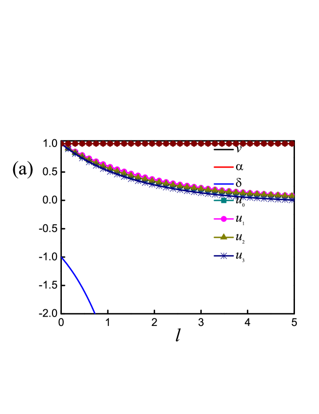
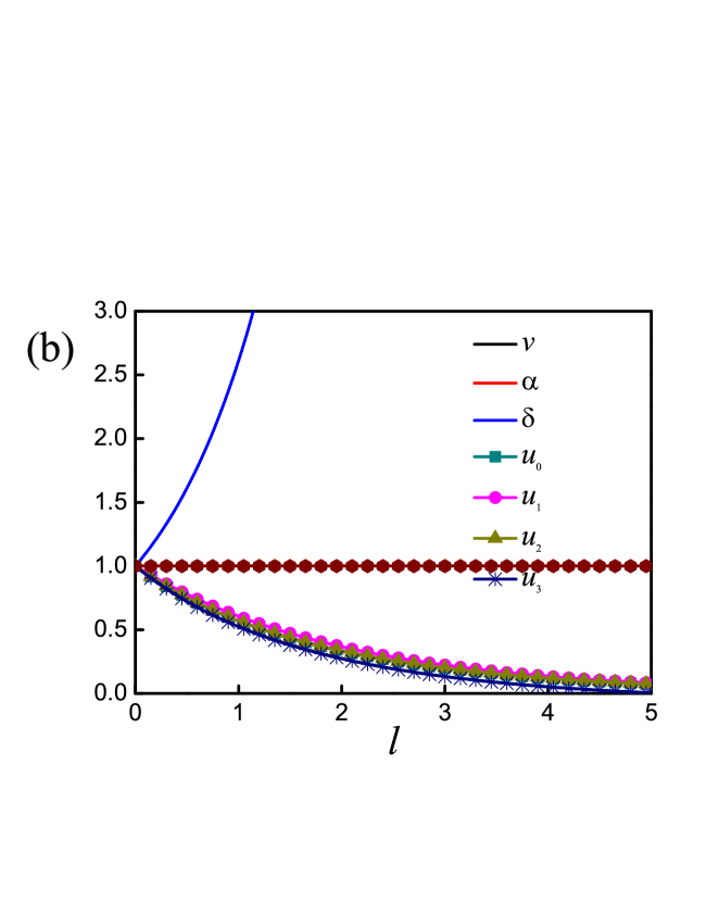
Figure 4: (Color online) Flows of interaction parameters due to the corrections from the four-fermion interactions. The initial value of $\delta$ is taken to be negative (a) or positive (b) and others equally.

Based on these information, we eventually achieve the effective theory for the presence of impurity by combing the effective action in Sec. III at clean limit and the fermion-impurity interaction (31),

$$S^{\prime}_{\mathrm{eff}} = S_{\mathrm{eff}}+S_{\mathrm{fd}}.$$ (32)

Paralleling the one-loop analysis for fermion propagator in Sec. III.2 and computing the one-loop fermion-impurity diagrams in Fig. 3 for the presence of random chemical potential, we find that the fermion propagator would gain a nontrivial revision from the fermion-impurity interaction, namely

$$\Sigma = \frac{\Delta v^{2}_{D}\mathcal{D}_{0}}{8\pi^{2}}(i\omega)l.$$ (33)

The other two sorts of fermion-impurity interactions both give rise to nonzero corrections by practicing similar procedures,

$$\Sigma = -\frac{\Delta v^{2}_{D}\mathcal{D}_{0}}{8\pi^{2}}(i\omega)l.$$ (34)

In such circumstance, we next can utilize these nontrivial corrections to produce certain nonzero anomalous fermion dimensions, which are list as

$$\eta^{\mathrm{chem}}_{f} = -\frac{\Delta v^{2}_{D}\mathcal{D}_{0}}{8\pi^{2}}=-\eta^{\mathrm{gaug}}_{f}=-\eta^{\mathrm{mass}}_{f}.$$ (35)

where the indexes $\mathrm{chem},\mathrm{gaug},\mathrm{mass}$ denote the random chemical potential, random gauge potential and random mass, representatively. These nonzero anomalous dimensions will be intensely instructive to derive the coupled flow equations of interaction parameters in next subsection, which are sharp contrast to a trivial value at clean limit in Eq. (13) Nersesyan1995NPB ; Huh2008PRB ; Wang2011PRB . In addition, the impurity strength can participate in the coupled RG evolutions as a new member and affect the revised evolutions of all correlated interaction parameters.

IV.2 Coupled flow equations in the presence of impurity

After carrying out the analogous steps in section III with employing the one-loop corrections in Appendix A.2, we consequently summarize the coupled flow equations of all related parameters in the presence of random chemical potential,

$$\left.\begin{array}[]{ll}\frac{dv}{dl}=\frac{\Delta v^{2}_{D}\mathcal{D}_{0}}{8\pi^{2}}v,\vspace{0.53cm}\\ \vspace{0.53cm}\frac{d\alpha}{dl}=\frac{\Delta v^{2}_{D}\mathcal{D}_{0}}{8\pi^{2}}\alpha,\\ \vspace{0.53cm}\frac{d\delta}{dl}=\left(1-\frac{u_{1}\mathcal{C}_{1}}{8\pi^{2}}+\frac{\Delta v^{2}_{D}\mathcal{D}_{0}}{8\pi^{2}}\right)\delta,\\ \vspace{0.53cm}\frac{du_{0}}{dl}=\frac{2(\Delta v^{2}_{D}\mathcal{D}_{0}-2\pi^{2})u_{0}-u_{0}(u_{2}+u_{3})(\mathcal{C}_{2}+\mathcal{C}_{3}-\mathcal{C}_{0})-u_{0}u_{1}(3\mathcal{C}_{2}+\mathcal{C}_{3}-\mathcal{C}_{0})-4\Delta v^{2}_{D}(\mathcal{D}_{2}+\mathcal{D}_{3})}{8\pi^{2}},\\ \vspace{0.53cm}\frac{du_{1}}{dl}=\frac{2(\Delta v^{2}_{D}\mathcal{D}_{0}-2\pi^{2})u_{1}-u_{1}(u_{2}+u_{3}-u_{0})(\mathcal{C}_{0}-\mathcal{C}_{2})-u_{1}(3u_{2}+u_{3}-u_{0})\mathcal{C}_{3}-\mathcal{C}_{2}(u^{2}_{0}+u^{2}_{1}+u^{2}_{2}+u^{2}_{3})+2\Delta v^{2}_{D}(\mathcal{D}_{2}-\mathcal{D}_{3})}{8\pi^{2}},\\ \vspace{0.53cm}\frac{du_{2}}{dl}=\frac{2(\Delta v^{2}_{D}\mathcal{D}_{0}-2\pi^{2})u_{2}-u_{2}(u_{1}+u_{3}-u_{0})(\mathcal{C}_{0}+\mathcal{C}_{2}-\mathcal{C}_{3})+2\Delta v^{2}_{D}(\mathcal{D}_{3}-\mathcal{D}_{2})}{8\pi^{2}},\\ \vspace{0.53cm}\frac{du_{3}}{dl}=\frac{2(\Delta v^{2}_{D}\mathcal{D}_{0}-2\pi^{2})u_{3}-u_{3}(u_{1}+u_{2}-u_{0})(\mathcal{C}_{0}+\mathcal{C}_{2}+\mathcal{C}_{3})+6\Delta v^{2}_{D}(\mathcal{D}_{2}+\mathcal{D}_{3})}{8\pi^{2}},\\ \vspace{0.53cm}\frac{dv_{D}}{dl}=\frac{\Delta v^{2}_{D}\mathcal{D}_{0}+2[\Delta v^{2}_{D}-(u_{0}+u_{1}+u_{2}+u_{3})](\mathcal{D}_{2}+\mathcal{D}_{3})}{8\pi^{2}}v_{D}.\end{array}\right.$$ (44)

In order to present more compact evolutions of the interaction parameters (44), we here have nominated four new coefficients that are designated as

$$\mathcal{D}_{0} = \int^{\frac{\pi}{2}}_{-\frac{\pi}{2}}d\theta\frac{2}{\alpha^{2}\cos^{2}\theta+v^{2}\sin^{2}\theta},$$ (45)

$$\mathcal{D}_{1} = \int^{\frac{\pi}{2}}_{-\frac{\pi}{2}}d\theta\frac{2\alpha\cos\theta}{\alpha^{2}\cos^{2}\theta+v^{2}\sin^{2}\theta},$$ (46)

$$\mathcal{D}_{2} = \int^{\frac{\pi}{2}}_{-\frac{\pi}{2}}d\theta\frac{2\alpha^{2}\cos^{2}\theta}{(\alpha^{2}\cos^{2}\theta+v^{2}\sin^{2}\theta)^{2}},$$ (47)

$$\mathcal{D}_{3} = \int^{\frac{\pi}{2}}_{-\frac{\pi}{2}}d\theta\frac{2v^{2}\sin^{2}\theta}{(\alpha^{2}\cos^{2}\theta+v^{2}\sin^{2}\theta)^{2}}.$$ (48)

The coupled flow equations for the presence of other two types of impurities can derived analogously and are provided in the Appendix B. In such situation, we can study the effects of these coupled flow equations that collect contribution from both four-fermion interaction and impurity on the low-energy behaviors of the semi-Dirac materials in the following section.

V Stability of the ground states against the fermionic interaction

We have already presented the coupled RG flow equations of correlated coupling parameters in Sec. III for the presence of fermion-fermion interactions. In the light of these running Eqs. (20)-(25), we are informed that all these interaction parameters participate in the coupled evolutions and mutually affect each other upon lowering energy scale. We subsequently concentrate on the fate of parameter $\delta$ in low-energy regime under taking into account one-loop interaction corrections.

Clearly, the parameter $\delta$ becomes energy-dependent and is coupled with the evolutions of other parameters via reading the information provided in Eqs. (20)-(25). To be specific, the parameter $\delta$ flows via decreasing the energy scale and it manifestly replies upon the coupling parameter $u_{1}$ and additionally collects the contribution from the parameters $u_{0}$, $u_{2}$, and $u_{3}$ owning to their closely coupled RG equations. As told in Ref. Saha2016PRB , the parameter $\delta$ is extremely crucial to pin down the ground state of the 2D SD system: (i) $\delta=0$, the spectrum is gapless with linear dispersion along $k_{y}$; (ii) $\delta<0$, it is a gapped system with a trivial insulating phase; and (iii) $\delta>0$, there exists two gapless Dirac nodal points at $(\pm\sqrt{\delta/\alpha},0)$ and this implies certain nontrivially topological state sets in. It is indeed that the system would choose one of these states and be stable while we begin with the noninteracting action (1) Saha2016PRB .

However, we would like to stress that, the evolution of parameter $\delta$ with lowering the energy scale, in apparently contrast to action (1), is reconstructed profoundly while the four-fermion interactions are switched on as presented in Eqs. (20)-(25). In addition, all interaction parameters are not independent but closely coupled with each other. In this respect, it is intensely instructive to ask whether the low-energy properties of parameter $\delta$ can be qualitatively modified by incorporating into the one-loop corrections due to the four-fermion interactions, namely whether these three ground states are stable against these short-range four-fermion interactions?

In order to response to these questions, we have to numerically analyze the coupled RG equations (20)-(25). To this end, we first take the initial value of parameter $\delta$ to be negative, i.e., $\delta(l=0)<0$ and rescale all the parameters by dividing their initial values, which are supposed an equal starting constant for unbiased consideration. After carrying out the numerical calculations of coupled Eqs. (20)-(25) with these initial conditions, we obtain interesting results as illustrated in Fig. 4(a). This result directly suggests that the semimetal state with $\delta<0$ is insensitive to the four-fermion interaction and stable in the low-energy regime. Similarly, we representatively assume the parameter $\delta$ to be positive initially and deliver the results after paralleling the previous steps as designated in Fig. 4(b). The qualitative results for the case $\delta(l=0)=0$ are analogous and not shown here. According to the tendency of evolutions upon decreasing the energy scale in Fig. 4, we are unambiguously told that the sign of parameter $\delta$ cannot be changed qualitatively by the fermion-fermion interactions. This thereafter indicates both the trivial insulating state and nontrivial topological state are considerable stable against the four-fermion interactions Saha2016PRB .

We stop here to present several comments on these numerical results. At tree level, we easily obtain that all of the quartic interaction parameters are irrelevant in the RG language after implementing the RG analysis of effective action, i.e., Eq. (4) Shankar1994RMP ; Huh2008PRB ; Wang2011PRB . In addition, the numerical calculations of one-loop coupled flow equations countenance this point as demonstrated in Fig. 4. In the spirt of momentum-shell RG theory Shankar1994RMP , this means that the fermion-fermion interaction parameters are irrelevant even to one-loop level and as a result the contribution from four-fermion interactions becomes less and less significant and finally vanishes at the lowest-energy limit Ramakrishnan1985RMP ; Nersesyan1995NPB ; Mirlin2008RMP . Consequently, these parameters cannot qualitatively destroy the ground sates of the 2D SD material. Since the low-energy states of 2D SD system are insensitive to these short-range four-fermion interaction, it is imperative to investigate the effects of impurities, which are well known to be always present in the real systems, and in particular interplay between four-fermion interaction and impurity on these states.

VI Low-energy behaviors affected by the interaction and impurity

Impurities are well-known one of most significant facets in producing a multitude of prominent phenomena of Fermi systems Ramakrishnan1985RMP ; Nersesyan1995NPB ; Mirlin2008RMP . Within this section, we are going to study and answer whether our previously basic results with switching on the four-fermion interactions at clean limit in the 2D SD system are robust under certain number of impurities and their competition with fermion-fermion interaction. In Fermi systems, there are three typical types of impurities, which are dubbed by random chemical potential, random mass, and random gauge potential Nersesyan1995NPB ; Stauber2005PRB ; Wang2011PRB . Without loss of generality, all these three sorts of impurities will be equally investigated. After taking into account the contribution for the presence of both four-fermion interaction and impurity, the coupled RG flow equations of interaction parameters are modified from Eq. (20)-(25) to Eq. 44, Eq. (91), and Eq. (100). Under such circumstances, we can expect the remarkably revised behavior of parameter $\delta$ in the low-energy regime.

VI.1 Interaction-impurity induced phase transition

To proceed, we endeavor to numerically calculate Eq. (44), Eq. (91), and Eq. (100) to check the energy-dependent properties against the impurity. At the outset, we consider the presence of random chemical potential with the coupled flow equations (44) and the other two cases will be followed.

In order to facilitate our analysis, we parallel the steps in Sec. V and initially let $\delta(l=0)=0$ and other parameters are assumed to own an equal starting value. Before moving further, we elucidate the information on the strength of impurity. For physical consideration, we introduce the impurity scattering rate to qualify the initial value of impurity strength as Coleman2015Book

$$\tau^{-1}\sim\frac{\Delta v^{2}_{D}}{\alpha},$$ (49)

where $\alpha$, $\Delta$ and $v_{D}$ are nominated in Eqs. (2), (29) and (30), representatively. In the sprit of the perturbative theory, we need to restrict the initial value of $\tau^{-1}(l=0)\equiv\tau^{-1}_{0}\leq\Lambda_{0}$. After carrying out the similarly numerical performance, we find that the parameter $\delta$ exhibits analogously compared to the pure-interaction case when the starting value of impurity scattering rate is considerable small, namely $\tau^{-1}_{0}$ is much smaller than $\Lambda_{0}$. In this case, the ground state of system is stable and the corresponding numerical results are not shown here. On the contrary, while the initial value of impurity scattering rate is large, for instance $\tau^{-1}_{0}>0.1\Lambda_{0}$, it is of particular interest that the sign of parameter $\delta$ with a negative starting value can be changed upon lowering the energy scale as displayed in Fig. 5.

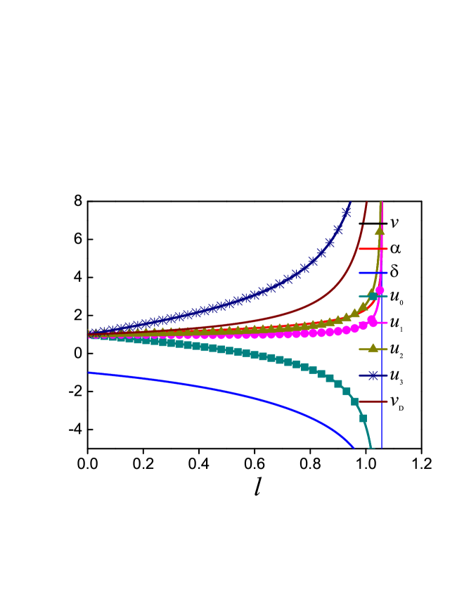
Figure 5: (Color online) Flows of parameters due to the corrections from the interplay between four-fermion interactions and random chemical potential. The sign of parameter $\delta$ is changed upon lowering the energy scale.

This apparently signals that the system undergoes a phase transition Fradkin2009PRL ; Vafek2012PRB ; Vafek2014PRB ; Wang2017QBCP ; Altland2006Book ; Vojta2003RPP ; Metzner2000PRL ; Metzner2000PRB ; Wang2014PRB ; Chubukov2010PRB ; Chubukov2012ARCMP ; Chubukov2016PRX . As shown in Fig. 5, it is interesting to point out that the fermionic coupling parameters are divergent at certain critical energy (dubbed by $l=l_{c}$). Guided by the spirt of momentum-shell RG Wilson1975RMP ; Polchinski9210046 ; Shankar1994RMP and phase transition theory Sachdev1999Book ; Altland2006Book ; Vojta2003RPP , we are informed, compared to the clean-limit case with only switching the four-fermion interactions in Sec. V, that the irrelevant fermion-fermion interaction parameters can be transferred to irrelevant relevant interaction couplings in the low-energy regime after collecting one-loop corrections due to the close interplay between four-fermion interactions and impurity. Generally, these irrelevant relevant parameters are responsible for the divergences of interaction parameters. A multitude of previous studies Fradkin2009PRL ; Vafek2012PRB ; Vafek2014PRB ; Wang2017QBCP ; Altland2006Book ; Vojta2003RPP ; Metzner2000PRL ; Metzner2000PRB ; Wang2014PRB ; Chubukov2010PRB ; Chubukov2012ARCMP ; Chubukov2016PRX reveal that these divergent coupling parameters are the evident signals of instability and phase transitions. Consequently, we infer that the intimate interplay between four-fermion interaction and impurity together triggers some phase transition in the low-energy regime. At this stage, a good candidate for our 2D SD material occurs, namely, a trivial insulator experiencing certain phase transition to become a nontrivial Dirac semimetal owning to the strong interplay between random chemical potential and fermion-fermion interactions.

Subsequently, we move to the cases for presence of random gauge potential and random mass via considering Eq. (91) and Eq. (100) in Appendix B. Paralleling the analysis for the random chemical potential indicates these two sorts of impurities share the qualitative results with the random chemical potential: while the impurity scattering rate is small, the ground states of 2D SD systems are strongly stable against the interplay between fermion-fermion interaction and impurities; however, the potential phase transition from a trivial insulator to a gapless Dirac nodal system would be generated by the random gauge potential or random mass if the initial value of scattering rate of impurity is adequate large, which is as the same order as the value in Fig. 5. The primary difference from the random chemical potential is that critical energy scales $E_{c}$ at which certain phase transition is generated are distributed into three distinct values. After performing both analogously numerical and theoretical studies, we are left with the orders of critical energy scales as

$$E^{\mathrm{chem}}_{c}<E^{\mathrm{mass}}_{c}<E^{\mathrm{gaug}}_{c}.$$ (50)

where $\mathrm{chem},\mathrm{mass},\mathrm{gaug}$ describes the random chemical potential, random mass and random gauge potential, representatively. As the numerical results are similar to the presence of random chemical potential, we do not provide them here.

Based on these analysis, we conclude that the ground states of 2D SD materials are qualitatively stable against all three types of impurities at a small impurity scattering rate, but certain phase transition can be generated under specific condition as exhibited in Fig. 5 while the initial value of impurity scattering rate exceeds certain critical value to make the fermion-fermion interaction parameters irrelevantly relevant and the interplay between four-fermion interaction and impurity remarkably significant.

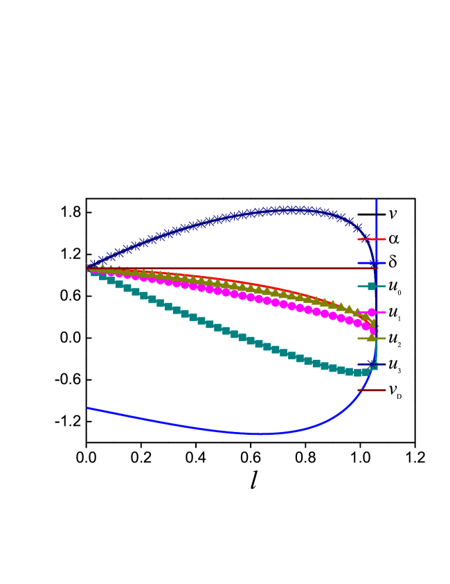
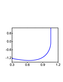
Figure 6: (Color online) Relatively fixed points of flows of parameters due to the corrections from the interplay between four-fermion interactions and random chemical potential. The initial values are followed by the Fig. 5 and the values of parameters are measured by $v_{D}$. Inset: evolution of parameter $\delta$ in the sign-change regime.

VI.2 Relatively fixed point and phase transition

Before closing the study of the impurity-induced phase transition, we would like to provide our comments on this particular phase transition, which is conventionally accompanied by the sign change of parameter $\delta$ shown in the last subsection.

To this end, we first need to seek the critical fixed point in the parameter space that is lined to the critical energy scale represented by $l_{c}$ (or $E_{c}$) at which the interaction couplings are divergent and instabilities take place Shankar1994RMP ; Vafek2012PRB ; Vafek2014PRB ; Metzner2000PRL ; Metzner2000PRB ; Chubukov2010PRB ; Chubukov2016PRX . Learning from Fig. 5 informs us that the interaction coupling parameters (or their absolute values) are increased quickly and finally divergent at certain critical energy scale. In order to make our analysis remain weak coupling, one can measure all of interaction couplings with one of them (no sign change) and try to obtain the relatively fixed point of their rations at this critical energy scale Shankar1994RMP ; Vafek2012PRB ; Vafek2014PRB . Motivated by this idea and after performing analogously numerical analysis, we produce the relative evolutions of interaction parameters and acquire our relatively fixed point, namely, $[(v,\alpha,u_{0},u_{1},u_{2},u_{3},u_{4},v_{D})/v_{D}]^{*}\approx(0,0,-5.0\times 10^{-4},9.0\times 10^{-5},2.4\times 10^{-4},1.2\times 10^{-3},1)$ by following the initial values of coupled flows in Fig. 5. In particular, we find that $[\delta/v_{D}]^{*}$ is substantially large and nearly divergent as presented in Fig. 6 in 2D SD system. Combing the evolutions of interaction parameters in Fig. 5 and Fig. 6, it singles out that the divergence of parameter $\delta$ at the critical energy scale should be intimately associated with the leading instability and simultaneously accompanied by a phase transition. Given the perturbative restriction of our momentum-shell RG framework Shankar1994RMP , we admit that our approach may gradually break down and even be invalid at $l\geq l_{c}$ as the $\delta(l_{c}+\delta l)$ goes towards the strong coupling. However, it is well proved that this analysis can conventionally provide constructive information for leading instability and potential phase transition of the fermionic systems via approaching the critical energy scale Fradkin2009PRL ; Vafek2012PRB ; Vafek2014PRB ; Wang2017QBCP ; Altland2006Book ; Vojta2003RPP ; Metzner2000PRL ; Metzner2000PRB ; Wang2014PRB ; Chubukov2010PRB ; Chubukov2012ARCMP ; Chubukov2016PRX . Under all these consideration, we are encouraged to infer that some phase transition must be trigged by the strong interplay between fermion-fermion interaction and impurity in the vicinity of the critical energy scale denoted by $l_{c}$.

In order to judge which instability is dominant or which phase transition should be taken place, we in principle need to calculate all of susceptibilities of potential instabilities allowed by the symmetries of related system around its relatively fixed point and pick up the leading one to be tied to the specific phase transition Vafek2012PRB ; Vafek2014PRB ; Metzner2000PRL ; Metzner2000PRB ; Chubukov2010PRB ; Chubukov2016PRX .

However, one usually, without loss of generality, can also directly read the primary type of phase transition from the evolutions of interaction parameters Chubukov2010PRB ; Chubukov2012ARCMP . Generally, the activated phase transition is linked to the largest parameter at the critical energy scale Chubukov2010PRB ; Chubukov2012ARCMP . As presented in Fig. 5 and Fig. 6, the parameter $\delta$ features the largest value at the critical energy scale. Additionally, the leading parameter $\delta$ is forced to go towards (positively) strong coupling at $l=l_{c}$. Hence one can expect it would be positive at the low-energy regime. Moreover, it clearly exhibits the sign change of the parameter $\delta$ upon approaching the critical energy scale as displayed in the inset figure of Fig. 6. In present study, we only try to put our focus on how the four-fermion interaction and impurity qualitatively influence the stabilities of the ground states of 2D SD systems. Therefore for the sake of simplicity we suggest that the 2D SD system experiences a phase transition from a trivial insulator to a nontrivial Dirac semimetal according to the spirt from Refs. Chubukov2010PRB ; Chubukov2012ARCMP caused by the interplay between random chemical potential and four-fermion interaction.

VI.3 Sign change and phase transition

To further clarify the implication of sign change, we, within this subsection, provide further discussions on the relationship between the sign change of parameter $\delta$ and phase transition. As studied in above two subsections, the $\delta=0$ corresponds to an unstable fixed point that is suggested to be linked to the phase transition. It is worth pointing out that the key ingredient producing the sign change of $\delta$ is the divergent quantum fluctuation at the phase transition point.

To be specific, we would like to emphasize, for physical consideration, the sign change of $\delta$ is not solely taken place but closely and intimately associated with the phase transition point at which the instability sets in accompanied concomitantly with the divergent susceptibilities at the critical energy scale. By approaching the quantum critical point (of the phase transition), the quantum fluctuations become stronger and stronger, and finally divergent at that point. These unusual behaviors enter into the coupled flow equations via the one-loop corrections and then greatly influence the value of right-hand side of flow equations (44) in the vicinity of phase transition point, such as the parameter $\delta$’s equation. As a result, the sign change and divergence of parameter $\delta$ are triggered simultaneously under certain initial conditions of four-fermion parameters and impurity strength.

For the mathematical consideration, we, for convenience, dub the right hand of flow equation of $\delta$ as the slope of the $\delta$ equation nominated by $S_{\delta}$ and assume the unstable fixed point takes place at $l_{c}$. If one starts from a $\delta_{0}<0$ with $S_{\delta_{0}}>0$, then $\delta$ gradually approaches the fixed point via lowering the energy scale. On the contrary, $\delta$ goes to the strong coupling once we begin from a $\delta_{0}>0$ still with $S_{\delta_{0}}>0$. This explicitly implies the single-direction tendency of a parameter can be realized and closely tied to the sign of $S_{\delta}$. To be concretely, if the sign of $S_{\delta}$ is the same while an infinitesimal perturbation is tuned, $l_{c}\rightarrow l\pm\delta l$, the sign change of unstable fixed point can be realized Herbut2007Book . Guided by above discussion, we can straightforwardly numerically examine the $S_{\delta}$ away from $l_{c}$ in current work (however the theoretical proof is hardly done for these complicatedly coupled flow equations (44)). Before going further, we would like to highlight that the ”initial state” should be understood as a relative notation. For instance, supposing the divergent behaviors set in at $l_{c}$, we can define the ”initial states” with $l^{\pm}_{0}\equiv l_{c}\pm\delta l$. To be specific, the evolution can follow the steps: (i) initially, $\delta$ starts from a negative value at $l^{+}_{0}$, and its absolute value decreases in that the numerical calculation of coupled RG equations indicates $S_{\delta}(l^{+}_{0})>0$; (ii) while $l\rightarrow l_{c}$ it goes nearly zero, but the zero point is an unstable fixed point impacted by the strong quantum fluctuation; (iii) then adding an infinitesimal increase with $l^{-}_{0}$, the slope can change qualitatively by the divergent quantum fluctuation still with $S_{\delta}(l^{-}_{0}>0)$ informed by the numerical evaluation, which breaks the balance of the zero point fixed point and the parameter is directly forced to the strong coupling.

To reiterate, the intimate relationship between the evolutions of coupled flow equations and strong quantum fluctuation yields to the singular behavior of the $\delta$’s RG equation, and eventually results in the the sign change and divergence of $\delta$ at phase transition point under certain initial conditions.

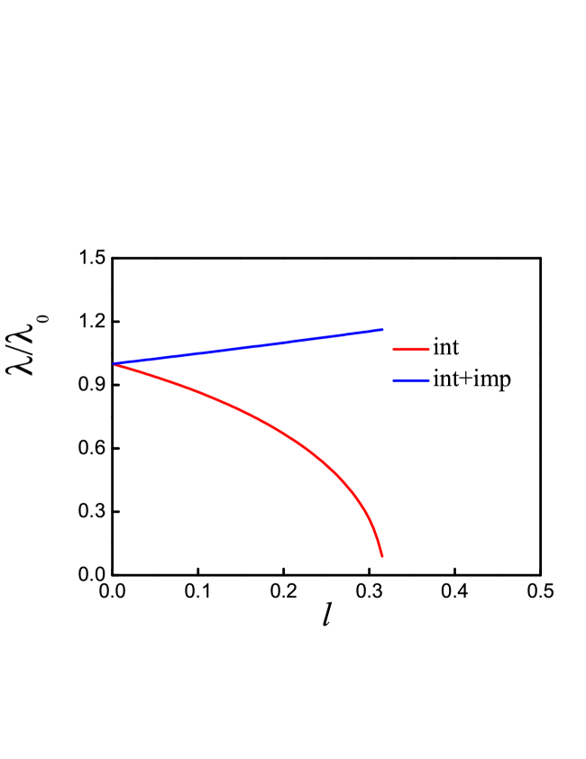
Figure 7: (Color online) Evolution of the distance ($\lambda/\lambda_{0}$) between two nodal points in the $\delta>0$ states in the presence of pure interaction ($\mathrm{int}$) and interaction+impruity ($\mathrm{int+imp}$) before approaching the critical energy scale.

VI.4 Distance of Dirac nodal points

In addition to the phase transition investigated in former parts of Sec. VI, we here display another interesting behavior triggered by the interplay between four-fermion interactions and impurity.

As addressed in Sec. II, the 2D SD material possesses two gapless Dirac nodal points for $\delta>0$, namely at $(\pm\sqrt{\frac{\delta}{\alpha}},0)$. Despite the gapless states with $\delta>0$ being considerably stable against the short-range four-fermion interaction or impurity (assuming the initial value of impurity scattering rate is not too large), the distance between these two Dirac nodal points may be varied by the four-fermion interaction or impurity. To proceed, their distance can be expressed as Saha2016PRB

$$\lambda=2\sqrt{\frac{\delta}{\alpha}}.$$ (51)

This straightforwardly indicates that the distance $\lambda$ flows upon lowering the energy scale as the correlated parameters both $\delta$ and $\alpha$ evolve and are coupled complicatedly with other interaction parameters along the coupled RG flow equations (20)-(25) or (44), (91) and (100). We therefore are forced to numerically analyze these coupled RG running equations to investigate the energy-dependent properties of the distance of Dirac nodal points $\lambda$. Before moving further, we here would like to stress that the following study is restricted to the energy scales which are larger than the critical energy scale represented by $l_{c}$.

We subsequently take the starting value of $\delta$ positive to ensure the starting state harbors two Dirac nodal points and other parameters to possess the similar values to Fig. 4’s. The corresponding numerical results of the energy-dependent distance for both cases are delineated in Fig. 7. We deduce that the four-fermion interaction can reduce the distance of Dirac nodal points after capturing the basic information from Fig. 7. On the contrary, the presence all three sorts of impurities would increase the distance $\lambda$ (as the difference among distinct types of impurities is negligible, we only leave one line for impurity in Fig. 7). As a consequence, we conclude that the distance of Dirac nodal points in the semimetal states of 2D SD system is sensitive to the four-fermion interaction or impurity, which representatively try to decrease or increase the distance $\lambda$ as depicted in Fig. 7. One may expect that the increase of distance of Dirac nodal point would be somehow harmful to the possibility of interplay between the gapless excitations in the low-energy regime. Hence, this result is qualitatively consistent with the conclusion in Sec. V and Sec. VI that the ground state of 2D SD system is stable against the four-fermion interaction and sensitive to the interplay between the four-fermion interaction and impurity.

VII Non-Fermi liquid behaviors

Based on our RG analysis in last several sections, the impurity indeed play a crucial role in pinning down the physical quantities in the low-energy regime. We finally investigate how the physical quantities behavior at the lowest-energy limit. In this section, we focus on the quasiparticle residue $Z_{f}$ and DOS of the quasiparticle. As the random chemical potential is a relevant parameter, our perturbative RG method may break down at the lowest-energy limit and thus cannot clearly present an answer to the fate of Landau quasiparticles Altland2002PR . Therefore, we here only focus on the random gauge potential and random mass.

At the outset, we study the residue $Z_{f}$, which can be introduced via

$$Z_{f}=\frac{1}{1-\frac{\partial\mathrm{Re}\Sigma^{\mathrm{R}}(\omega)}{\partial\omega}},$$ (52)

where $\mathrm{Re}\Sigma^{\mathrm{R}}$ represents the real part of retarded fermion self-energy. It is worth pointing out that whether the notation of quasiparticle is well- or unwell- defined (Fermi liquid or non-Fermi liquid) is closely associated with this renormalization factor $Z_{f}$. On one side, a finite $Z_{f}$ corresponds to the Fermi liquid. On the other, the non-Fermi liquid (behavior) is usually accompanied by the residue $Z_{f}\rightarrow 0$. Subsequently, we can derive the evolution of $Z_{f}$ depending on the energy scale after performing momentum-shell RG analysis and collecting the one-loop corrections to anomalous dimensions Eq. (33) and Eq. (35), namely Ludwig1994PRB ; Xu2008PRB ; WLZ2016NJP ; Wang2017PRB2

$$\frac{dZ_{f}}{dl}=-\eta^{i}_{f}Z_{f},$$ (53)

where $i=\mathrm{gaug},\mathrm{mass}$ as shown in Eq. (35) representatively correspond to the random gauge potential and random mass. By carrying the numerical analysis, we find that $\lim_{l\rightarrow\infty}Z_{f}=0$ for both the random gauge potential and random mass, this straightforwardly signals that the Dirac fermions are no longer well-defined Landau quasiparticles. As a result, non-Fermi liquid behaviors have been activated.

Additionally, we move to the DOS of the quasiparticle, whose flow $\rho$ under RG analysis can be expressed as  Ludwig1994PRB ; WLZ2016NJP for the 2D Dirac semimetal,

$$\frac{d\ln\rho(\omega)}{d\ln(\omega)}=\frac{1+\eta^{i}_{f}}{1-\eta^{i}_{f}},$$ (54)

here again $i=\mathrm{gaug},\mathrm{mass}$ denotes distinct types of disorders. This implies the DOS $\rho(\omega)\sim\omega$ for the clean and noninteracting 2D Dirac semimetal. In order to examine the low-energy behaviors of the DOS in the presence of impurities, we perform the numerical analysis after combining Eq. (54) and coupled flow equations for the presence of impurities, namely, Eq. (91) and Eq. (100) and subsequently are informed that the DOS at the lowest-energy regime deviates from the linear behavior $\rho(\omega)\sim\omega$ due to the intimate interplay between four-fermion interactions and random gauge potential or random mass. This is therefore also a signature of non-Fermi liquid behavior.

VIII Summary

In summary, we have carefully investigated the effects of four-fermion interactions, impurities, and the interplay between fermionic interactions and impurities on the ground states of 2D SD materials. In order to capture more information of physical ingredients in the low-energy regime, all allowed types of short-range four-fermion interactions by symmetries and three kinds of impurities, namely random chemical potential, random mass, and random gauge potential Nersesyan1995NPB ; Stauber2005PRB ; Wang2011PRB , are included and treated on the same footing by means of utilizing the momentum-shell RG theory Wilson1975RMP ; Polchinski9210046 ; Shankar1994RMP . The coupled flow equations for all related interaction parameters are derived after carrying out the standard RG analysis Wilson1975RMP ; Polchinski9210046 ; Shankar1994RMP for both the pure interaction and presence of impurity, which are employed to study the low-energy behaviors of 2D SD systems affected by the interplay between the fermionic interaction and impurity. After performing both analytic and numerical consideration of these coupled flow equations, whether and how theses fermion-fermion interactions and impurity impact the low-energy properties of the 2D SD materials are fully studied and presented.

To be specific, we first consider the clean limit case with only switching on four sorts of four-fermion interactions. After analyzing the evolutions of the related interaction parameters upon lowering the energy scales, we clearly display that all of four-fermion parameters are irrelevant in the RG language Shankar1994RMP ; Huh2008PRB ; Wang2011PRB to one-loop level. This indicates that the contribution from four-fermion interactions becomes less and less significant and finally vanishes at the lowest-energy limit Shankar1994RMP . Based on these theoretical and numerical studies, we therefore conclude that both the trivial insulating state and gapless semimetal state are considerably stable against the short-range fermion-fermion interactions. However, while the impurity is taken into account simultaneously, the close interplay between four-fermion interaction and impurity can play a crucial role in determining the ground state of 2D SD system. Concretely, these irrelevantly fermionic parameters can be transferred to irrelevant relevant after collecting the corrections from interplay between interaction and impurity. Additionally, if the initial value of impurity scattering exceeds certain critical value, we find that the quartic interaction couplings are divergent and sign of parameter $\delta$ can be changed concomitantly at a critical energy scale. This conventionally suggests that some phase transition would be triggered Fradkin2009PRL ; Vafek2012PRB ; Vafek2014PRB ; Wang2017QBCP ; Altland2006Book ; Vojta2003RPP ; Metzner2000PRL ; Metzner2000PRB ; Wang2014PRB ; Chubukov2010PRB ; Chubukov2012ARCMP ; Chubukov2016PRX . For our 2D SD material, we expect that the system experiences a phase transition from a trivial insulator to a nontrivial Dirac, which is activated together by the interplay between four-fermion interactions and impurities in the low-energy regime under specific conditions although the states are qualitatively stable against all three types of impurities Fradkin2009PRL ; Vafek2012PRB ; Vafek2014PRB ; Wang2017QBCP ; Altland2006Book ; Vojta2003RPP ; Metzner2000PRL ; Metzner2000PRB ; Wang2014PRB ; Chubukov2010PRB ; Chubukov2012ARCMP ; Chubukov2016PRX .

In addition, we find that the distance of two Dirac nodal points in this 2D SD material is sensitive to the four-fermion interactions or impurities. On one side, all three sorts of impurities are helpful to increase the distance of Dirac nodal points. On the other, the four-fermion interaction is preferable to decreases it. This interesting result is expected to be in line with the basic conclusion in Sec. V and Sec. VI that the ground state of 2D SD system is stable against the four-fermion interaction and sensitive to the interplay between the four-fermion interaction and impurity. Furthermore, several deviations from Fermi liquid behaviors Altland2002PR , such as the quasiparticle residue $Z_{f}$ and the DOS, are displayed at the lowest-energy limit caused by the interplay between the four-fermion interactions and random gauge potential or random mass. These exotic properties are manifest signals of non-Fermi liquid behaviors.

Before closing this section we would like to present brief comments on the long-range fermion-fermion interaction. The long-range interactions may be possibly formally rewritten as Boettcher2016PRB ; Hirata2016NComm

$$S_{\mathrm{int}} = \sum^{3}_{a=0}u_{a}\int\frac{d\omega_{1}d\omega_{2}}{(2\pi)^{2}}\int\frac{d^{2}\mathbf{k}_{1}d^{2}\mathbf{k}_{2}}{(2\pi)^{4}}\Psi^{\dagger}(\omega_{1},\mathbf{k}_{1})\sigma_{a}$$ (55)

$$\times\Psi(\omega_{1},\mathbf{k}_{1})\Psi^{\dagger}(\omega_{2},\mathbf{k}_{2})\sigma_{a}\Psi(\omega_{2},\mathbf{k}_{2}),$$

which would give rise to totally different coupled evolutions of related parameters in that one independent momentum and frequency would be vanished. Accordingly, this interaction is expected to trigger more interesting behaviors. However, one central problem is that the long-range interactions are hardly present due to all kinds of screenings. In particular, we take into account the effects of impurity scatterings, which are unavoidably allowed in real systems and are very detrimental for the long-range interactions. Under this circumstance, it seems inappropriate to study the long-range interaction in this work, which we leave for a future study hypothesizing the restricted conditions of presence of long-range interaction being satisfied.

Finally, we expect that impeding experiments will be achieved to detect and verify whether there exists the analogous phase transition from the gapped to gapless phases in the 2D SD materials, the variance for distance of Dirac nodal points in the gapless phase, and also possibly non-Fermi liquid behaviors at the low-energy regime. This may be profitable for us to further understand and uncover the unique properties of 2D SD materials and even instructive to motivate the new materials by virtue of many experimental methods LCJS2009PRL ; Beenakker2009PRL ; Rosenberg2010PRL ; Hasan2011Science ; Bahramy2012NC ; Viyuela2012PRB ; Bardyn2012PRL ; Garate2003PRL ; Oka2009PRB ; Lindner2011NP ; Gedik2013Science ; CBHR2016PRL .

Appendix A One-loop corrections

A.1 Four-fermion couplings at clean limit

According to Fig. 2(i) and (ii), integrating out the fast modes of fermionic fields and carrying out the standard momentum-shell RG framework Shankar1994RMP ; Huh2008PRB ; She2010PRB ; Wang2011PRB ; Vafek2012PRB by means of utilizing the RG transformations of the momenta (7), energy (8), and fields (9) give rise to the one-loop corrections at clean limit

$$\delta S^{i+ii}_{u_{0}} = \left[\frac{-u_{0}(u_{0}+u_{1}+u_{2}+u_{3})(\mathcal{C}_{2}+\mathcal{C}_{3}-\mathcal{C}_{0})}{8\pi^{2}}l\right]\int^{+\infty}_{-\infty}\frac{d\omega_{1}d\omega_{2}d\omega_{3}}{(2\pi)^{3}}\int^{b}\frac{d^{2}\mathbf{k}_{1}d^{2}\mathbf{k}_{2}d^{2}\mathbf{k}_{3}}{(2\pi)^{6}}$$ (56)

$$\times\Psi^{\dagger}(\omega_{1},\mathbf{k}_{1})\sigma_{0}\Psi(\omega_{2},\mathbf{k}_{2})\Psi^{\dagger}(\omega_{3},\mathbf{k}_{3})\sigma_{0}\Psi(\omega_{1}+\omega_{2}-\omega_{3},\mathbf{k}_{1}+\mathbf{k}_{2}-\mathbf{k}_{3}),$$

$$\delta S^{iii}_{u_{0}} = \left[\frac{u^{2}_{0}(\mathcal{C}_{2}+\mathcal{C}_{3}-\mathcal{C}_{0})}{8\pi^{2}}l\right]\int^{+\infty}_{-\infty}\frac{d\omega_{1}d\omega_{2}d\omega_{3}}{(2\pi)^{3}}\int^{b}\frac{d^{2}\mathbf{k}_{1}d^{2}\mathbf{k}_{2}d^{2}\mathbf{k}_{3}}{(2\pi)^{6}}\Psi^{\dagger}(\omega_{1},\mathbf{k}_{1})\sigma_{0}\Psi(\omega_{2},\mathbf{k}_{2})$$ (57)

$$\times\Psi^{\dagger}(\omega_{3},\mathbf{k}_{3})\sigma_{0}\Psi(\omega_{1}+\omega_{2}-\omega_{3},\mathbf{k}_{1}+\mathbf{k}_{2}-\mathbf{k}_{3}),$$

$$\delta S^{iv}_{u_{0}} = \left[\frac{\mathcal{C}_{0}(u^{2}_{0}+u^{2}_{1}+u^{2}_{2}+u^{2}_{3})-2\mathcal{C}_{2}u_{0}u_{1}-2\mathcal{C}_{3}u_{0}u_{2}}{16\pi^{2}}l\right]\int^{+\infty}_{-\infty}\frac{d\omega_{1}d\omega_{2}d\omega_{3}}{(2\pi)^{3}}\int^{b}\frac{d^{2}\mathbf{k}_{1}d^{2}\mathbf{k}_{2}d^{2}\mathbf{k}_{3}}{(2\pi)^{6}}$$ (58)

$$\times\Psi^{\dagger}(\omega_{1},\mathbf{k}_{1})\sigma_{0}\Psi(\omega_{2},\mathbf{k}_{2})\Psi^{\dagger}(\omega_{3},\mathbf{k}_{3})\sigma_{0}\Psi(\omega_{1}+\omega_{2}-\omega_{3},\mathbf{k}_{1}+\mathbf{k}_{2}-\mathbf{k}_{3}),$$

$$\delta S^{v}_{u_{0}} = \left[\frac{-\mathcal{C}_{0}(u^{2}_{0}+u^{2}_{1}+u^{2}_{2}+u^{2}_{3})-2\mathcal{C}_{2}u_{0}u_{1}+2\mathcal{C}_{3}u_{0}u_{2}}{16\pi^{2}}l\right]\int^{+\infty}_{-\infty}\frac{d\omega_{1}d\omega_{2}d\omega_{3}}{(2\pi)^{3}}\int^{b}\frac{d^{2}\mathbf{k}_{1}d^{2}\mathbf{k}_{2}d^{2}\mathbf{k}_{3}}{(2\pi)^{6}}$$ (59)

$$\times\Psi^{\dagger}(\omega_{1},\mathbf{k}_{1})\sigma_{0}\Psi(\omega_{2},\mathbf{k}_{2})\Psi^{\dagger}(\omega_{3},\mathbf{k}_{3})\sigma_{0}\Psi(\omega_{1}+\omega_{2}-\omega_{3},\mathbf{k}_{1}+\mathbf{k}_{2}-\mathbf{k}_{3}),$$

for one-loop corrections to $u_{0}$,

$$\delta S^{i+ii}_{u_{1}} = \left[\frac{u_{1}(u_{0}+u_{1}-u_{2}-u_{3})(\mathcal{C}_{0}-\mathcal{C}_{2}+\mathcal{C}_{3})}{8\pi^{2}}l\right]\int^{+\infty}_{-\infty}\frac{d\omega_{1}d\omega_{2}d\omega_{3}}{(2\pi)^{3}}\int^{b}\frac{d^{2}\mathbf{k}_{1}d^{2}\mathbf{k}_{2}d^{2}\mathbf{k}_{3}}{(2\pi)^{6}}$$ (60)

$$\times\Psi^{\dagger}(\omega_{1},\mathbf{k}_{1})\sigma_{1}\Psi(\omega_{2},\mathbf{k}_{2})\Psi^{\dagger}(\omega_{3},\mathbf{k}_{3})\sigma_{1}\Psi(\omega_{1}+\omega_{2}-\omega_{3},\mathbf{k}_{1}+\mathbf{k}_{2}-\mathbf{k}_{3}),$$

$$\delta S^{iii}_{u_{1}} = \left[\frac{u^{2}_{1}(\mathcal{C}_{2}-\mathcal{C}_{3}-\mathcal{C}_{0})}{8\pi^{2}}l\right]\int^{+\infty}_{-\infty}\frac{d\omega_{1}d\omega_{2}d\omega_{3}}{(2\pi)^{3}}\int^{b}\frac{d^{2}\mathbf{k}_{1}d^{2}\mathbf{k}_{2}d^{2}\mathbf{k}_{3}}{(2\pi)^{6}}$$ (61)

$$\times\Psi^{\dagger}(\omega_{1},\mathbf{k}_{1})\sigma_{1}\Psi(\omega_{2},\mathbf{k}_{2})\Psi^{\dagger}(\omega_{3},\mathbf{k}_{3})\sigma_{1}\Psi(\omega_{1}+\omega_{2}-\omega_{3},\mathbf{k}_{1}+\mathbf{k}_{2}-\mathbf{k}_{3}),$$

$$\delta S^{iv}_{u_{1}} = \left[\frac{2\mathcal{C}_{0}u_{0}u_{1}-\mathcal{C}_{2}(u^{2}_{0}+u^{2}_{1}+u^{2}_{2}+u^{2}_{3})-2\mathcal{C}_{3}u_{1}u_{2}}{16\pi^{2}}l\right]\int^{+\infty}_{-\infty}\frac{d\omega_{1}d\omega_{2}d\omega_{3}}{(2\pi)^{3}}\int^{b}\frac{d^{2}\mathbf{k}_{1}d^{2}\mathbf{k}_{2}d^{2}\mathbf{k}_{3}}{(2\pi)^{6}}$$ (62)

$$\times\Psi^{\dagger}(\omega_{1},\mathbf{k}_{1})\sigma_{1}\Psi(\omega_{2},\mathbf{k}_{2})\Psi^{\dagger}(\omega_{3},\mathbf{k}_{3})\sigma_{1}\Psi(\omega_{1}+\omega_{2}-\omega_{3},\mathbf{k}_{1}+\mathbf{k}_{2}-\mathbf{k}_{3}),$$

$$\delta S^{v}_{u_{1}} = \left[\frac{-2\mathcal{C}_{0}u_{0}u_{1}-\mathcal{C}_{2}(u^{2}_{0}+u^{2}_{1}+u^{2}_{2}+u^{2}_{3})-2\mathcal{C}_{3}u_{1}u_{2}}{16\pi^{2}}l\right]\int^{+\infty}_{-\infty}\frac{d\omega_{1}d\omega_{2}d\omega_{3}}{(2\pi)^{3}}\int^{b}\frac{d^{2}\mathbf{k}_{1}d^{2}\mathbf{k}_{2}d^{2}\mathbf{k}_{3}}{(2\pi)^{6}}$$ (63)

$$\times\Psi^{\dagger}(\omega_{1},\mathbf{k}_{1})\sigma_{1}\Psi(\omega_{2},\mathbf{k}_{2})\Psi^{\dagger}(\omega_{3},\mathbf{k}_{3})\sigma_{1}\Psi(\omega_{1}+\omega_{2}-\omega_{3},\mathbf{k}_{1}+\mathbf{k}_{2}-\mathbf{k}_{3}),$$

for one-loop corrections to $u_{1}$,

$$\delta S^{i+ii}_{u_{2}} = \left[\frac{u_{2}(u_{0}-u_{1}+u_{2}-u_{3})(\mathcal{C}_{0}+\mathcal{C}_{2}-\mathcal{C}_{3})}{8\pi^{2}}l\right]\int^{+\infty}_{-\infty}\frac{d\omega_{1}d\omega_{2}d\omega_{3}}{(2\pi)^{3}}\int^{b}\frac{d^{2}\mathbf{k}_{1}d^{2}\mathbf{k}_{2}d^{2}\mathbf{k}_{3}}{(2\pi)^{6}}$$ (64)

$$\times\Psi^{\dagger}(\omega_{1},\mathbf{k}_{1})\sigma_{2}\Psi(\omega_{2},\mathbf{k}_{2})\Psi^{\dagger}(\omega_{3},\mathbf{k}_{3})\sigma_{2}\Psi(\omega_{1}+\omega_{2}-\omega_{3},\mathbf{k}_{1}+\mathbf{k}_{2}-\mathbf{k}_{3}),$$

$$\delta S^{iii}_{u_{2}} = \left[\frac{u^{2}_{2}(\mathcal{C}_{3}-\mathcal{C}_{2}-\mathcal{C}_{0})}{8\pi^{2}}l\right]\int^{+\infty}_{-\infty}\frac{d\omega_{1}d\omega_{2}d\omega_{3}}{(2\pi)^{3}}\int^{b}\frac{d^{2}\mathbf{k}_{1}d^{2}\mathbf{k}_{2}d^{2}\mathbf{k}_{3}}{(2\pi)^{6}}$$ (65)

$$\times\Psi^{\dagger}(\omega_{1},\mathbf{k}_{1})\sigma_{2}\Psi(\omega_{2},\mathbf{k}_{2})\Psi^{\dagger}(\omega_{3},\mathbf{k}_{3})\sigma_{2}\Psi(\omega_{1}+\omega_{2}-\omega_{3},\mathbf{k}_{1}+\mathbf{k}_{2}-\mathbf{k}_{3}),$$

$$\delta S^{iv}_{u_{2}} = \left[\frac{2\mathcal{C}_{0}u_{0}u_{2}-2\mathcal{C}_{2}u_{1}u_{2}-\mathcal{C}_{3}(u^{2}_{0}+u^{2}_{1}+u^{2}_{2}+u^{2}_{3})}{16\pi^{2}}l\right]\int^{+\infty}_{-\infty}\frac{d\omega_{1}d\omega_{2}d\omega_{3}}{(2\pi)^{3}}\int^{b}\frac{d^{2}\mathbf{k}_{1}d^{2}\mathbf{k}_{2}d^{2}\mathbf{k}_{3}}{(2\pi)^{6}}$$ (66)

$$\times\Psi^{\dagger}(\omega_{1},\mathbf{k}_{1})\sigma_{2}\Psi(\omega_{2},\mathbf{k}_{2})\Psi^{\dagger}(\omega_{3},\mathbf{k}_{3})\sigma_{2}\Psi(\omega_{1}+\omega_{2}-\omega_{3},\mathbf{k}_{1}+\mathbf{k}_{2}-\mathbf{k}_{3}),$$

$$\delta S^{v}_{u_{2}} = \left[\frac{-2\mathcal{C}_{0}u_{0}u_{2}+2\mathcal{C}_{2}u_{1}u_{2}+\mathcal{C}_{3}(u^{2}_{0}+u^{2}_{1}+u^{2}_{2}+u^{2}_{3})}{16\pi^{2}}l\right]\int^{+\infty}_{-\infty}\frac{d\omega_{1}d\omega_{2}d\omega_{3}}{(2\pi)^{3}}\int^{b}\frac{d^{2}\mathbf{k}_{1}d^{2}\mathbf{k}_{2}d^{2}\mathbf{k}_{3}}{(2\pi)^{6}}$$ (67)

$$\times\Psi^{\dagger}(\omega_{1},\mathbf{k}_{1})\sigma_{2}\Psi(\omega_{2},\mathbf{k}_{2})\Psi^{\dagger}(\omega_{3},\mathbf{k}_{3})\sigma_{2}\Psi(\omega_{1}+\omega_{2}-\omega_{3},\mathbf{k}_{1}+\mathbf{k}_{2}-\mathbf{k}_{3}),$$

for one-loop corrections to $u_{2}$, and

$$\delta S^{i+ii}_{u_{3}} = \left[\frac{u_{3}(u_{0}-u_{1}-u_{2}+u_{3})(\mathcal{C}_{0}+\mathcal{C}_{2}+\mathcal{C}_{3})}{8\pi^{2}}l\right]\int^{+\infty}_{-\infty}\frac{d\omega_{1}d\omega_{2}d\omega_{3}}{(2\pi)^{3}}\int^{b}\frac{d^{2}\mathbf{k}_{1}d^{2}\mathbf{k}_{2}d^{2}\mathbf{k}_{3}}{(2\pi)^{6}}$$ (68)

$$\times\Psi^{\dagger}(\omega_{1},\mathbf{k}_{1})\sigma_{3}\Psi(\omega_{2},\mathbf{k}_{2})\Psi^{\dagger}(\omega_{3},\mathbf{k}_{3})\sigma_{3}\Psi(\omega_{1}+\omega_{2}-\omega_{3},\mathbf{k}_{1}+\mathbf{k}_{2}-\mathbf{k}_{3}),$$

$$\delta S^{iii}_{u_{3}} = \left[\frac{u^{2}_{3}(-\mathcal{C}_{3}-\mathcal{C}_{2}-\mathcal{C}_{0})}{8\pi^{2}}l\right]\int^{+\infty}_{-\infty}\frac{d\omega_{1}d\omega_{2}d\omega_{3}}{(2\pi)^{3}}\int^{b}\frac{d^{2}\mathbf{k}_{1}d^{2}\mathbf{k}_{2}d^{2}\mathbf{k}_{3}}{(2\pi)^{6}}$$ (69)

$$\times\Psi^{\dagger}(\omega_{1},\mathbf{k}_{1})\sigma_{3}\Psi(\omega_{2},\mathbf{k}_{2})\Psi^{\dagger}(\omega_{3},\mathbf{k}_{3})\sigma_{3}\Psi(\omega_{1}+\omega_{2}-\omega_{3},\mathbf{k}_{1}+\mathbf{k}_{2}-\mathbf{k}_{3}),$$

$$\delta S^{iv}_{u_{3}} = \left[\frac{(2\mathcal{C}_{0}u_{0}u_{3}-2\mathcal{C}_{2}u_{1}u_{3}-2\mathcal{C}_{3}u_{2}u_{3})}{16\pi^{2}}l\right]\int^{+\infty}_{-\infty}\frac{d\omega_{1}d\omega_{2}d\omega_{3}}{(2\pi)^{3}}\int^{b}\frac{d^{2}\mathbf{k}_{1}d^{2}\mathbf{k}_{2}d^{2}\mathbf{k}_{3}}{(2\pi)^{6}}$$ (70)

$$\times\Psi^{\dagger}(\omega_{1},\mathbf{k}_{1})\sigma_{3}\Psi(\omega_{2},\mathbf{k}_{2})\Psi^{\dagger}(\omega_{3},\mathbf{k}_{3})\sigma_{3}\Psi(\omega_{1}+\omega_{2}-\omega_{3},\mathbf{k}_{1}+\mathbf{k}_{2}-\mathbf{k}_{3}),$$

$$\delta S^{v}_{u_{3}} = \left[\frac{(-2\mathcal{C}_{0}u_{0}u_{3}+2\mathcal{C}_{2}u_{1}u_{3}-2\mathcal{C}_{3}u_{2}u_{3})}{16\pi^{2}}l\right]\int^{+\infty}_{-\infty}\frac{d\omega_{1}d\omega_{2}d\omega_{3}}{(2\pi)^{3}}\int^{b}\frac{d^{2}\mathbf{k}_{1}d^{2}\mathbf{k}_{2}d^{2}\mathbf{k}_{3}}{(2\pi)^{6}}$$ (71)

$$\times\Psi^{\dagger}(\omega_{1},\mathbf{k}_{1})\sigma_{3}\Psi(\omega_{2},\mathbf{k}_{2})\Psi^{\dagger}(\omega_{3},\mathbf{k}_{3})\sigma_{3}\Psi(\omega_{1}+\omega_{2}-\omega_{3},\mathbf{k}_{1}+\mathbf{k}_{2}-\mathbf{k}_{3}),$$

for one-loop corrections to $u_{3}$.

Figure 8: One-loop corrections to the fermion interacting couplings in the presence of impurities. The dashed line indicates the four-fermion interaction and the wave line represents the impurity. fermion interaction and the wave line represents the impurity. To be specific, the subfigures (i)-(v) and (vi)-(xiii) respectively capture the contributions from purely four-fermion interaction and mixtures of both four-fermion interaction and impurity.

A.2 Four-fermion couplings in the presence of impurity

Due to the interplay between fermion-fermion interaction and impurity, we also need to take into account the corrections from fermion-impurity interaction besides the fermion-fermion interaction contributions provided in Appendix A.1. In the presence of impurities, all one-loop Feynman diagrams contributing to the four-fermion couplings are demonstrated in Fig. 8. As the subfigures (i)-(v) of Fig. 8 have already been evaluated in Appendix A.1, we subsequently will focus on the left subfigures of Fig. 8 one by one, i.e, subfigures (vi)-(xiii). For the presence of random chemical potential, we can obtain the one-loop corrections

$$\delta S^{vi+vii}_{u_{0},\gamma=\sigma_{0}} = \left[\frac{u_{0}\Delta v^{2}_{D}}{4\pi^{2}}\Bigl{(}\mathcal{D}_{2}+\mathcal{D}_{3}\Bigr{)}l\right]\int\frac{d\omega_{1}d\omega_{2}d\omega_{3}}{(2\pi)^{3}}\int^{b}\frac{d^{2}\mathbf{k}_{1}d^{2}\mathbf{k}_{2}d^{2}\mathbf{k}_{3}}{(2\pi)^{6}}$$ (72)

$$\times\Psi^{\dagger}(\omega_{1},\mathbf{k}_{1})\sigma_{0}\Psi(\omega_{2},\mathbf{k}_{2})\Psi^{\dagger}(\omega_{3},\mathbf{k}_{3})\sigma_{0}\Psi(\omega_{1}+\omega_{2}-\omega_{3},\mathbf{k}_{1}+\mathbf{k}_{2}-\mathbf{k}_{3}),$$

$$\delta S^{x+xi}_{u_{0},\gamma=\sigma_{0}} = \left[\frac{-u_{0}\Delta v^{2}_{D}}{\pi^{2}}\Bigl{(}\mathcal{D}_{2}+\mathcal{D}_{3}\Bigr{)}l\right]\int\frac{d\omega_{1}d\omega_{2}d\omega_{3}}{(2\pi)^{3}}\int^{b}\frac{d^{2}\mathbf{k}_{1}d^{2}\mathbf{k}_{2}d^{2}\mathbf{k}_{3}}{(2\pi)^{6}}$$ (73)

$$\times\Psi^{\dagger}(\omega_{1},\mathbf{k}_{1})\sigma_{0}\Psi(\omega_{2},\mathbf{k}_{2})\Psi^{\dagger}(\omega_{3},\mathbf{k}_{3})\sigma_{0}\Psi(\omega_{1}+\omega_{2}-\omega_{3},\mathbf{k}_{1}+\mathbf{k}_{2}-\mathbf{k}_{3}),$$

$$\delta S^{xii+xiii}_{u_{0},\gamma=\sigma_{0}} = \left[\frac{u_{0}\Delta v^{2}_{D}}{4\pi^{2}}\Bigl{(}\mathcal{D}_{2}+\mathcal{D}_{3}\Bigr{)}l\right]\int\frac{d\omega_{1}d\omega_{2}d\omega_{3}}{(2\pi)^{3}}\int^{b}\frac{d^{2}\mathbf{k}_{1}d^{2}\mathbf{k}_{2}d^{2}\mathbf{k}_{3}}{(2\pi)^{6}}$$ (74)

$$\times\Psi^{\dagger}(\omega_{1},\mathbf{k}_{1})\sigma_{0}\Psi(\omega_{2},\mathbf{k}_{2})\Psi^{\dagger}(\omega_{3},\mathbf{k}_{3})\sigma_{0}\Psi(\omega_{1}+\omega_{2}-\omega_{3},\mathbf{k}_{1}+\mathbf{k}_{2}-\mathbf{k}_{3}),$$

$$\delta S^{vi+vii}_{u_{1},\gamma=\sigma_{0}} = \left[\frac{u_{1}\Delta v^{2}_{D}(\mathcal{D}_{2}-\mathcal{D}_{3})}{4\pi^{2}}l\right]\int\frac{d\omega_{1}d\omega_{2}d\omega_{3}}{(2\pi)^{3}}\int^{b}\frac{d^{2}\mathbf{k}_{1}d^{2}\mathbf{k}_{2}d^{2}\mathbf{k}_{3}}{(2\pi)^{6}}$$ (75)

$$\times\Psi^{\dagger}(\omega_{1},\mathbf{k}_{1})\sigma_{1}\Psi(\omega_{2},\mathbf{k}_{2})\Psi^{\dagger}(\omega_{3},\mathbf{k}_{3})\sigma_{1}\Psi(\omega_{1}+\omega_{2}-\omega_{3},\mathbf{k}_{1}+\mathbf{k}_{2}-\mathbf{k}_{3}),$$

$$\delta S^{vi+vii}_{u_{2},\gamma=\sigma_{0}} = \left[\frac{u_{2}\Delta v^{2}_{D}(\mathcal{D}_{3}-\mathcal{D}_{2})}{4\pi^{2}}l\right]\int\frac{d\omega_{1}d\omega_{2}d\omega_{3}}{(2\pi)^{3}}\int^{b}\frac{d^{2}\mathbf{k}_{1}d^{2}\mathbf{k}_{2}d^{2}\mathbf{k}_{3}}{(2\pi)^{6}}$$ (76)

$$\times\Psi^{\dagger}(\omega_{1},\mathbf{k}_{1})\sigma_{2}\Psi(\omega_{2},\mathbf{k}_{2})\Psi^{\dagger}(\omega_{3},\mathbf{k}_{3})\sigma_{2}\Psi(\omega_{1}+\omega_{2}-\omega_{3},\mathbf{k}_{1}+\mathbf{k}_{2}-\mathbf{k}_{3}),$$

$$\delta S^{vi+vii}_{u_{3},\gamma=\sigma_{0}} = \left[\frac{-u_{3}\Delta v^{2}_{D}}{4\pi^{2}}\Bigl{(}\mathcal{D}_{2}+\mathcal{D}_{3}\Bigr{)}l\right]\int\frac{d\omega_{1}d\omega_{2}d\omega_{3}}{(2\pi)^{3}}\int^{b}\frac{d^{2}\mathbf{k}_{1}d^{2}\mathbf{k}_{2}d^{2}\mathbf{k}_{3}}{(2\pi)^{6}}$$ (77)

$$\times\Psi^{\dagger}(\omega_{1},\mathbf{k}_{1})\sigma_{3}\Psi(\omega_{2},\mathbf{k}_{2})\Psi^{\dagger}(\omega_{3},\mathbf{k}_{3})\sigma_{3}\Psi(\omega_{1}+\omega_{2}-\omega_{3},\mathbf{k}_{1}+\mathbf{k}_{2}-\mathbf{k}_{3}),$$

$$\delta S^{viii}_{u_{3},\gamma=\sigma_{0}} = \left[\frac{u_{3}\Delta v^{2}_{D}}{4\pi^{2}}\Bigl{(}\mathcal{D}_{2}\mathrm{Tr}(\sigma_{1}\sigma_{a})\mathrm{Tr}(\sigma_{a}\sigma_{1})+\mathcal{D}_{3}\mathrm{Tr}(\sigma_{2}\sigma_{a})\mathrm{Tr}(\sigma_{a}\sigma_{2})\Bigr{)}l\right]\int\frac{d\omega_{1}d\omega_{2}d\omega_{3}}{(2\pi)^{3}}\int^{b}\frac{d^{2}\mathbf{k}_{1}d^{2}\mathbf{k}_{2}d^{2}\mathbf{k}_{3}}{(2\pi)^{6}}$$ (78)

$$\times\Psi^{\dagger}(\omega_{1},\mathbf{k}_{1})\sigma_{3}\Psi(\omega_{2},\mathbf{k}_{2})\Psi^{\dagger}(\omega_{3},\mathbf{k}_{3})\sigma_{3}\Psi(\omega_{1}+\omega_{2}-\omega_{3},\mathbf{k}_{1}+\mathbf{k}_{2}-\mathbf{k}_{3}).$$

Figure 9: One-loop corrections to the fermion-impurity interaction in the presence of impurities. The dashed line indicates the four-fermion interaction and the wave line represents the impurity.

We would like to emphasize that all of the subfigures in Fig. 8 that are not mentioned above have no any contributions. For the presence of random gauge potential and random mass, one can derive the corrections similarly, which are not shown here.

A.3 Fermion-impurity coupling

We finally study the one-loop corrections to the interplay between four-fermion interaction and impurity, namely the fermion-impurity coupling, as illustrated in Fig. 9. After carrying out analytical calculations in the spirt of momentum-shell RG approach Shankar1994RMP ; Huh2008PRB ; She2010PRB ; Wang2011PRB ; Vafek2012PRB , we list the results as follows for the presence of all three types of impurities,

$$\delta S_{\gamma=\sigma_{0}} = \left\{\frac{v_{D}[\Delta v^{2}_{D}-(u_{0}+u_{1}+u_{2}+u_{3})](\mathcal{D}_{2}+\mathcal{D}_{3})}{4\pi^{2}}l\right\}\int\frac{d\omega}{(2\pi)}\int^{b}\frac{d^{2}\mathbf{k}d^{2}\mathbf{k^{\prime}}}{(2\pi)^{4}}$$ (79)

$$\times\Psi^{\dagger}(\omega,\mathbf{k})\sigma_{b}\Psi(\omega,\mathbf{k^{\prime}})D(\mathbf{k}-\mathbf{k^{\prime}}),$$

$$\delta S_{\gamma=\sigma_{1}} = \left\{\frac{v_{D}[\Delta v^{2}_{D}-(u_{0}+u_{1}-u_{2}-u_{3})](\mathcal{D}_{2}-\mathcal{D}_{3})}{4\pi^{2}}l\right\}\int\frac{d\omega}{(2\pi)}\int^{b}\frac{d^{2}\mathbf{k}d^{2}\mathbf{k^{\prime}}}{(2\pi)^{4}}$$ (80)

$$\times\Psi^{\dagger}(\omega,\mathbf{k})\sigma_{b}\Psi(\omega,\mathbf{k^{\prime}})D(\mathbf{k}-\mathbf{k^{\prime}}),$$

$$\delta S_{\gamma=\sigma_{3}} = \left\{\frac{v_{D}[(u_{0}-u_{1}-u_{2}+u_{3})-\Delta v^{2}_{D}](\mathcal{D}_{2}+\mathcal{D}_{3})}{4\pi^{2}}l\right\}\int\frac{d\omega}{(2\pi)}\int^{b}\frac{d^{2}\mathbf{k}d^{2}\mathbf{k^{\prime}}}{(2\pi)^{4}}$$ (81)

$$\times\Psi^{\dagger}(\omega,\mathbf{k})\sigma_{b}\Psi(\omega,\mathbf{k^{\prime}})D(\mathbf{k}-\mathbf{k^{\prime}}),$$

$$\delta S_{\gamma=\sigma_{2}} = \left\{\frac{v_{D}(u_{0}-u_{1}+u_{2}-u_{3}-\Delta v^{2}_{D})(\mathcal{D}_{2}-\mathcal{D}_{3})}{4\pi^{2}}l\right\}\int\frac{d\omega}{(2\pi)}\int^{b}\frac{d^{2}\mathbf{k}d^{2}\mathbf{k^{\prime}}}{(2\pi)^{4}}$$ (82)

$$\times\Psi^{\dagger}(\omega,\mathbf{k})\sigma_{b}\Psi(\omega,\mathbf{k^{\prime}})D(\mathbf{k}-\mathbf{k^{\prime}}),$$

where the Pauli matrix $\gamma=\sigma_{0}$, $\gamma=\sigma_{2}$, and $\gamma=\sigma_{1,3}$ respectively correspond to the random chemical potential, random mass and random gauge potential.

Appendix B Coupled flow equations for the presence of impurities

By virtue of paralleling the analysis of coupled RG equations in Sec. IV for the random chemical potential, the coupled flow equations for the presence of random gauge potential can be derived after performing the standard procedures of momentum-shell RG framework Shankar1994RMP ; Huh2008PRB ; She2010PRB ; Wang2011PRB ; Vafek2012PRB ,

$$\left.\begin{array}[]{ll}\frac{dv}{dl}=-\frac{\Delta v^{2}_{D}\mathcal{D}_{0}}{8\pi^{2}}v,\vspace{0.539cm}\\ \vspace{0.539cm}\frac{d\alpha}{dl}=\left(-1-\frac{\Delta v^{2}_{D}\mathcal{D}_{0}}{8\pi^{2}}\right)\alpha,\\ \vspace{0.539cm}\frac{d\delta}{dl}=\left(1-\frac{u_{1}\mathcal{C}_{1}}{8\pi^{2}}-\frac{\Delta v^{2}_{D}\mathcal{D}_{0}}{8\pi^{2}}\right)\delta,\\ \vspace{0.539cm}\frac{du_{0}}{dl}=\frac{-2(\Delta v^{2}_{D}\mathcal{D}_{0}+4\pi^{2})u_{0}-u_{0}(u_{2}+u_{3})(\mathcal{C}_{2}+\mathcal{C}_{3}-\mathcal{C}_{0})-u_{0}u_{1}(3\mathcal{C}_{2}+\mathcal{C}_{3}-\mathcal{C}_{0})+2\Delta v^{2}_{D}(2\mathcal{D}_{2}+\mathcal{D}_{3})}{8\pi^{2}},\\ \vspace{0.539cm}\frac{du_{1}}{dl}=\frac{-2(\Delta v^{2}_{D}\mathcal{D}_{0}+4\pi^{2})u_{1}-u_{1}(u_{2}+u_{3}-u_{0})(\mathcal{C}_{0}-\mathcal{C}_{2})-u_{1}(3u_{2}+u_{3}-u_{0})\mathcal{C}_{3}-\mathcal{C}_{2}(u^{2}_{0}+u^{2}_{1}+u^{2}_{2}+u^{2}_{3})+2\Delta v^{2}_{D}(2\mathcal{D}_{3}-\mathcal{D}_{2})}{8\pi^{2}},\\ \vspace{0.539cm}\frac{du_{2}}{dl}=\frac{-2(\Delta v^{2}_{D}\mathcal{D}_{0}+4\pi^{2})u_{2}-u_{2}(u_{1}+u_{3}-u_{0})(\mathcal{C}_{0}+\mathcal{C}_{2}-\mathcal{C}_{3})+\Delta v^{2}_{D}(3\mathcal{D}_{2}-2\mathcal{D}_{3})}{8\pi^{2}},\\ \vspace{0.539cm}\frac{du_{3}}{dl}=\frac{-2(\Delta v^{2}_{D}\mathcal{D}_{0}+4\pi^{2})u_{3}-u_{3}(u_{1}+u_{2}-u_{0})(\mathcal{C}_{0}+\mathcal{C}_{2}+\mathcal{C}_{3})+2\Delta v^{2}_{D}(3\mathcal{D}_{2}+2\mathcal{D}_{3})}{8\pi^{2}},\\ \vspace{0.539cm}\frac{dv_{D}}{dl}=\frac{2[(u_{3}-u_{1})\mathcal{D}_{2}+(u_{0}-u_{2}-\Delta v^{2}_{D})\mathcal{D}_{3}]-\Delta v^{2}_{D}\mathcal{D}_{0}}{8\pi^{2}}v_{D},\end{array}\right.$$ (91)

and finally carrying out analogous steps gives rise to the energy-dependent RG evolutions for presence of random mass,

$$\left.\begin{array}[]{ll}\frac{dv}{dl}=-\frac{\Delta v^{2}_{D}\mathcal{D}_{0}}{8\pi^{2}}v,\vspace{0.539cm}\\ \vspace{0.539cm}\frac{d\alpha}{dl}=\left(-1-\frac{\Delta v^{2}_{D}\mathcal{D}_{0}}{8\pi^{2}}\right)\alpha,\\ \vspace{0.539cm}\frac{d\delta}{dl}=\left(1-\frac{u_{1}\mathcal{C}_{1}}{8\pi^{2}}-\frac{\Delta v^{2}_{D}\mathcal{D}_{0}}{8\pi^{2}}\right)\delta,\\ \vspace{0.539cm}\frac{du_{0}}{dl}=\frac{-2(\Delta v^{2}_{D}\mathcal{D}_{0}+4\pi^{2})u_{0}-u_{0}(u_{2}+u_{3})(\mathcal{C}_{2}+\mathcal{C}_{3}-\mathcal{C}_{0})-u_{0}u_{1}(3\mathcal{C}_{2}+\mathcal{C}_{3}-\mathcal{C}_{0})+2\Delta v^{2}_{D}(\mathcal{D}_{2}+\mathcal{D}_{3})}{8\pi^{2}},\\ \vspace{0.539cm}\frac{du_{1}}{dl}=\frac{-2(\Delta v^{2}_{D}\mathcal{D}_{0}+4\pi^{2})u_{1}-u_{1}(u_{2}+u_{3}-u_{0})(\mathcal{C}_{0}-\mathcal{C}_{2})-u_{1}(3u_{2}+u_{3}-u_{0})\mathcal{C}_{3}-\mathcal{C}_{2}(u^{2}_{0}+u^{2}_{1}+u^{2}_{2}+u^{2}_{3})+2\Delta v^{2}_{D}(\mathcal{D}_{3}-\mathcal{D}_{2})}{8\pi^{2}},\\ \vspace{0.539cm}\frac{du_{2}}{dl}=\frac{-2(\Delta v^{2}_{D}\mathcal{D}_{0}+4\pi^{2})u_{2}-u_{2}(u_{1}+u_{3}-u_{0})(\mathcal{C}_{0}+\mathcal{C}_{2}-\mathcal{C}_{3})+6\Delta v^{2}_{D}(\mathcal{D}_{2}-\mathcal{D}_{3})}{8\pi^{2}},\\ \vspace{0.539cm}\frac{du_{3}}{dl}=\frac{-2(\Delta v^{2}_{D}\mathcal{D}_{0}+4\pi^{2})u_{3}-u_{3}(u_{1}+u_{2}-u_{0})(\mathcal{C}_{0}+\mathcal{C}_{2}+\mathcal{C}_{3})+2\Delta v^{2}_{D}(\mathcal{D}_{2}+\mathcal{D}_{3})}{8\pi^{2}},\\ \vspace{0.539cm}\frac{dv_{D}}{dl}=\frac{2\left[(u_{0}-u_{1}+u_{2}-u_{3})-\Delta v^{2}_{D}\right](\mathcal{D}_{2}-\mathcal{D}_{3})-\Delta v^{2}_{D}\mathcal{D}_{0}}{8\pi^{2}}v_{D},\end{array}\right.$$ (100)

where the coefficients $\mathcal{C}_{i}$ and $\mathcal{D}_{i}$, $i=0,1,2,3$ have been defined in the maintext, namely Eqs. (12), (26)-(28), and Eqs. (45)-(48).

References

- (1) K. S. Novoselov, A. K. Geim, S. V. Morozov, D. Jiang, M. I. Katsnelson, I. V. Grigorieva, S. V. Dubonos, and A. A. Firsov, Nature (London) 438, 197 (2005).
- (2) A. H. Castro Neto, F. Guinea, N. M. R. Peres, K. S. Novoselov, and A. K. Geim, Rev. Mod. Phys. 81, 109 (2009).
- (3) L. Fu, C. L. Kane, and E. J. Mele, Phys. Rev. Lett. 98, 106803 (2007).
- (4) R. Roy, Phys. Rev. B 79, 195322 (2009).
- (5) J. E. Moore, Nature (London) 464, 194 (2010).
- (6) M. Z. Hasan and C. L. Kane, Rev. Mod. Phys. 82, 3045 (2010).
- (7) X. -L. Qi and S. -C. Zhang, Rev. Mod. Phys. 83, 1057 (2011).
- (8) S. -Q. Sheng, Dirac Equation in Condensed Matter (Springer, Berlin, 2012).
- (9) B. A. Bernevig and T. L. Hughes, Topological Insulators and Topological Superconductors (Princeton University Press, Princeton, NJ, 2013); Topological Insulators, edited by M. Franz and L. Molenkamp, Contemporary Concepts of Condensed Matter Science Vol. 6 (Elsevier, Amsterdam, 2013).
- (10) A. A. Burkov, Leon Balents Phys. Rev. Lett. 107, 127205 (2011).
- (11) K. -Yu Yang, Y. -Ming Lu, Ying Ran Phys. Rev. B 84, 075129 (2011).
- (12) X. -G. Wan, A. M. Turner, A. Vishwanath, and S. Y. Savrasov, Phys. Rev. B 83, 205101 (2011).
- (13) X. Huang, L. Zhao, Y. Long, P. Wang, D. Chen, Z. Yang, H. Liang, M. Xue, H. Weng, Z. Fang, X. Dai, and G. Chen, Phys. Rev. X 5, 031023 (2015).
- (14) S. Y. Xu, I. Belopolski, N. Alidoust, M. Neupane, G. Bian, C. -L. Zhang, R. Sankar, G. -Q. Chang, Z. -J. Yuan, C. -C. Lee, S. -M. Huang, H. Zheng, J. Ma, D. S. Sanchez, B. -K. Wang, A. Bansil, F. -C. Chou, P. P. Shibayev, H. Lin, S. Jia, and M. Z. Hasan, Science 349, 613 (2015).
- (15) S. -Y. Xu, N. Alidoust, I. Belopolski, Z. -J. Yuan, G. Bian, T. -R. Chang, H. Zheng, V. N. Strocov, D. S. Sanchez, G.- Q. Chang, C.- L. Zhang, D. -X. Mou, Y. Wu, L. -N. Huang, C. -C. Lee, S. -M. Huang, B. -K. Wang, A. Bansil, H. -T. Jeng, T. Neupert, A. Kaminski, H. Lin, S. Jia, and M. Z. Hasan , Nat. Phys. 11, 748 (2015).
- (16) B. Q. Lv, N. Xu, H. M. Weng, J. Z. Ma, P. Richard, X. C. Huang, L. X. Zhao, G. F. Chen, C. E. Matt, F. Bisti, V. N. Strocov, J. Mesot, Z. Fang, X. Dai, T. Qian, M. Shi and H. Ding, Nat. Phys. 11, 724 (2015).
- (17) H. Weng, C. Fang, Z. Fang, B. A. Bernevig, X. Dai, Phys. Rev. X 5, 011029 (2015).
- (18) Z. -J. Wang, Y. Sun, X. -Q. Chen, C. Franchini, G. Xu, H. -M. Weng, X. Dai, and Z. Fang, Phys. Rev. B 85, 195320 (2012).
- (19) S. -M. Young, S. Zaheer, J. -C. Teo, C. -L. Kane, E. -J. Mele, and A. -M. Rappe, Phys. Rev. Lett. 108, 140405 (2012).
- (20) J. -A. Steinberg, S. -M. Young, S. Zaheer, C. -L. Kane, E. -J. Mele, and A. -M. Rappe, Phys. Rev. Lett. 112, 036403 (2014).
- (21) Z. K. Liu, J. Jiang, B. Zhou, Z. J. Wang, Y. Zhang, H. M. Weng, D. Prabhakaran, S -K. Mo, H. Peng, P. Dudin, T. Kim, M. Hoesch, Z. Fang, X. Dai, Z. X. Shen, D. L. Feng, Z. Hussain and Y. L. Chen, Nat. Mater. 13, 677 (2014).
- (22) Z. K. Liu, B. Zhou, Y. Zhang, Z. J. Wang, H. M. Weng, D. Prabhakaran, S. -K. Mo, Z. X. Shen, Z. Fang, X. Dai, Z. Hussain, Y. L. Chen, Science 343, 864 (2014).
- (23) J. Xiong, S. K. Kushwaha, T. Liang, J. W. Krizan, M. Hirschberger, W. Wang, R. J. Cava, N. P. Ong, Science 350, 413 (2015).
- (24) Y. Hasegawa, R. Konno, H. Nakano, and M. Kohmoto, Phys. Rev. B 74, 033413 (2006).
- (25) S. Katayama, A. Kobayashi, and Y. Suzumura, J. Phys. Soc. Jpn. 75, 054705 (2006).
- (26) P. Dietl, F. Piechon, and G. Montambaux, Phys. Rev. Lett. 100, 236405 (2008).
- (27) V. Pardo and W. E. Pickett, Phys. Rev. Lett. 102, 166803 (2009).
- (28) P. Delplace and G. Montambaux, Phys. Rev. B 82, 035438 (2010).
- (29) Y. Wu, Opt. Express 22, 1906 (2014).
- (30) S. Banerjee, R. R. P. Singh, V. Pardo, and W. E. Pickett, Phys. Rev. Lett. 103, 016402 (2009).
- (31) K. Saha, Phys. Rev. B 94, 081103(R) (2016).
- (32) B. Uchoa and K. Seo, Phys. Rev. B 96, 220503 (2017).
- (33) A. Altland, B. D. Simons, M. R. Zirnbauer, Phys. Rep. 359, 283 (2002).
- (34) P. A. Lee, N. Nagaosa, X. -G. Wen, Rev. Mod. Phys. 78, 17 (2006).
- (35) E. Fradkin, S. A. Kivelson, M. J. Lawler, J. P. Eisenstein, A. P. Mackenzie, Annu. Rev. Condens. Matter Phys. 1, 153 (2010).
- (36) S. Das Sarma, S. Adam, E. H. Hwang, E. Rossi, Rev. Mod. Phys. 83, 407 (2011).
- (37) S. Sachdev, Quantum Phase Transitions, (Cambridge University Press, second edition, Cambridge, 2011).
- (38) V. N. Kotov, B. Uchoa, V. M. Pereira, F. Guinea, A. H. Castro Neto, Rev. Mod. Phys. 84, 1067 (2012).
- (39) P. A. Lee, T. V. Ramakrishnan, Rev. Mod. Phys. 57, 287 (1985).
- (40) A. A. Nersesyan, A. M. Tsvelik, F. Wenger, Nucl. Phys. B 438 561 (1995) .
- (41) F. Evers and A. D. Mirlin, Rev. Mod. Phys. 80, 1355 (2008).
- (42) D. V. Efremov, M. M. Korshunov, O. V. Dolgov, A. A. Golubov, and P. J. Hirschfeld, Phys. Rev. B 84, 180512 (2011).
- (43) D. V. Efremov, A. A. Golubov, and O. V. Dolgov, New J. Phys. 15, 013002 (2013).
- (44) M. M. Korshunov, D. V. Efremov, A. A. Golubov, O. V. Dolgov, Phys. Rev. B 90, 134517 (2014).
- (45) H. -H. Hung, A. Barr, E. Prodan, and G. A. Fiete, Phys. Rev. B 94, 235132 (2016).
- (46) R. Nandkishore, J. Maciejko, D. A. Huse, and S. L. Sondhi, Phys. Rev. B 87, 174511 (2013).
- (47) I. -D. Potirniche, J. Maciejko, R. Nandkishore, and S. L. Sondhi, Phys. Rev. B 90, 094516 (2014).
- (48) R. M. Nandkishore, S. A. Parameswaran, Phys. Rev. B 95, 205106 (2017).
- (49) B. Roy, S. Das Sarma, Phys. Rev. B 94, 115137 (2016).
- (50) B. Roy, Y. Alavirad, and J. D. Sau, Phys. Rev. Lett. 94, 227002 (2017).
- (51) B. Roy, R. -J. Slager, and V. Juricic, arXiv: 1610.08973 (2016).
- (52) B. Roy , V. Juricic, and S. Das Sarma, Sci. Rep. 6, 32446 (2016).
- (53) T. Stauber, F. Guinea, and M. A. H. Vozmediano, Phys. Rev. B 71, 041406(R) (2005).
- (54) J. Wang, G. -Z. Liu, and H. Kleinert, Phys. Rev. B 83, 214503 (2011).
- (55) J. Wang, Phys. Rev. B 87, 054511 (2013).
- (56) I. L. Aleiner, K. B. Efetov, Phys. Rev. Lett. 97, 236801 (2006).
- (57) M. S. Foster, I. L. Aleiner, Phys. Rev. B 77, 195413 (2008).
- (58) Y. -L. Lee and Y. -W. Lee, Phys. Rev. B 96, 045115 (2017).
- (59) K. G. Wilson, Rev. Mod. Phys. 47 773 (1975).
- (60) J. Polchinski, arXiv: hep-th/9210046 (1992).
- (61) R. Shankar, Rev. Mod. Phys. 66, 129 (1994).
- (62) Y. Huh, S. Sachdev, Phys. Rev. B 78, 064512 (2008).
- (63) K. Sun, H. Yao, E. Fradkin, and S. A. Kivelson, Phys. Rev. Lett. 103, 046811 (2009).
- (64) V. Cvetkovic, R. E. Throckmorton, and O. Vafek, Phys. Rev. B 86, 075467 (2012).
- (65) J. M. Murray and O. Vafek, Phys. Rev. B 89, 201110(R) (2014).
- (66) J. Wang, C. Ortix, J. van den Brink, and D. V. Efremov, Phys. Rev. B 96, 201104(R) (2017).
- (67) A. Altland and B. Simons, Condensed Matter Field Theory (Cambridge University Press, Cambridge, 2006).
- (68) M. Vojta, Rep. Prog. Phys. 66, 2069 (2003).
- (69) C. J. Halboth and W. Metzner, Phys. Rev. Lett. 85, 5162 (2000).
- (70) C. J. Halboth and W. Metzner, Phys. Rev. B 61, 7364 (2000).
- (71) J. Wang, A. Eberlein, and W. Metzner, 89, 121116(R) (2014).
- (72) S. Maiti and A. V. Chubukov, Phys. Rev. B 82, 214515 (2010).
- (73) A. V. Chubukov, Annu. Rev. Condens. Matter Phys. 3, 57 (2012).
- (74) A. V. Chubukov, M. Khodas, and R. M. Fernandes, Phys. Rev. X 6, 041045 (2016).
- (75) H. Huang, Z. Liu, H. Zhang,W. Duan, and D. Vanderbilt, Phys. Rev. B 92, 161115 (2015).
- (76) E. -A. Kim, M. J. Lawler, P. Oreto, S. Sachdev, E. Fradkin, and S. A. Kivelson, Phys. Rev. B 77, 184514 (2008).
- (77) J. -H She, J Zaanen, A. R. Bishop, and A. V. Balatsky, Phys. Rev. B 82, 165128 (2010).
- (78) J. -H. She, M. J. Lawler, and E.-A. Kim, Phys. Rev. B 92, 035112 (2015).
- (79) B. Roy, P. Goswami, and J. D. Sau, Phys. Rev. B 94, 041101(R) (2016).
- (80) J. Wang and G. -Z. Liu, New J. Phys. 13, 073039 (2013).
- (81) J. Wang and G. -Z. Liu, Phys. Rev. D 90, 125015 (2014).
- (82) J. Wang and G. -Z. Liu, Phys. Rev. B 92, 184510 (2015).
- (83) J. Wang, G. -Z. Liu, D. V. Efremov, and J. van den Brink, Phys. Rev. B 95, 024511 (2017).
- (84) P. Coleman, Introduction to Many Body Physics (Cambridge University Press, 2015).
- (85) I. Herbut, A Modern Approach toCritical Phenomena, (Cambridge University Press, Cambridge, 2007).
- (86) A. W. W. Ludwig, M. P. A. Fisher, R. Shankar, and G. Grinstein, Phys. Rev. B 50, 7526 (1994).
- (87) C. Xu, Y. Qi, and S. Sachdev, Phys. Rev. B 78, 134507 (2008).
- (88) J. -R.Wang, G.-Z. Liu, and C. -J. Zhang, New J. Phys. 18, 073023 (2016).
- (89) J. Wang, P. -L. Zhao, J. -R.Wang, and G.-Z. Liu, Phys. Rev. B 95, 054507 (2017).
- (90) I. Boettcher, I. F. Herbut, Phys. Rev. B 93, 205138 (2016).
- (91) M. Hirata, K. Ishikawa, K. Miyagaw, M. Tamura, C. Berthier, D. Basko, A. Kobayashi, G. Matsuno, and K. Kanoda, Nat. Commun. 7, 12666 (2016).
- (92) J. Li, R. -L. Chu, J. K. Jain, and S. -Q. Shen, Phys. Rev. Lett. 102, 136806 (2009).
- (93) C. W. Groth, M. Wimmer, A. R. Akhmerov, J. Tworzydlo, and C. W. J. Beenakker, Phys. Rev. Lett. 103, 196805 (2009).
- (94) H. -M. Guo, G. Rosenberg, G. Refael, and M. Franz, Phys. Rev. Lett. 105, 216601 (2010).
- (95) S. -Y. Xu, Y. Xia, L. A. Wray, S. Jia, F. Meier, J. H. Dil, J. Osterwalder, B. Slomski, A. Bansil, H. Lin, R. J. Cava, and M. Z. Hasan, Science 332, 560 (2011).
- (96) M. Bahramy, B-J. Yang, R. Arita, and N. Nagaosa, Nat. Commun. 3, 679 (2012).
- (97) O. Viyuela, A. Rivas, and M. A. Martin-Delgado, Phys. Rev. B 86, 155140 (2012).
- (98) C. -E. Bardyn, M. A. Baranov, E. Rico, A. Imamoglu, P. Zoller, and S. Diehl, Phys. Rev. Lett. 109, 130402 (2012).
- (99) I. Garate, Phys. Rev. Lett. 110, 046402 (2013).
- (100) T. Oka and H. Aoki, Phys. Rev. B 79, 081406 (2009).
- (101) N. H. Lindner, G. Refael, and V. Galitski, Nat. Phys. 7, 490 (2011).
- (102) Y. H. Wang, H. Steinberg, P. Jarillo-Herrero, and N. Gedik, Science 342, 453 (2013).
- (103) C. -K. Chan, P. A. Lee, K. S. Burch, J. H. Han, and Y. Ran, Phys. Rev. Lett. 116, 026805 (2016).