OGLE-2017-BLG-1522: A giant planet around a brown dwarf located in the Galactic bulge

Abstract

We report the discovery of a giant planet in the OGLE-2017-BLG-1522 microlensing event. The planetary perturbations were clearly identified by high-cadence survey experiments despite the relatively short event timescale of $t_{\rm E}\sim 7.5$ days. The Einstein radius is unusually small, $\theta_{\rm E}=0.065\,$mas, implying that the lens system either has very low mass or lies much closer to the microlensed source than the Sun, or both. A Bayesian analysis yields component masses $(M_{\rm host},M_{\rm planet})=(46_{-25}^{+79},0.75_{-0.40}^{+1.26})~{}M_{\rm J}$ and source-lens distance $D_{\rm LS}=0.99_{-0.54}^{+0.91}~{}{\rm kpc}$, implying that this is a brown-dwarf/Jupiter system that probably lies in the Galactic bulge, a location that is also consistent with the relatively low lens-source relative proper motion $\mu=3.2\pm 0.5~{}{\rm mas}~{}{\rm yr^{-1}}$. The projected companion-host separation is $0.59_{-0.11}^{+0.12}~{}{\rm AU}$, indicating that the planet is placed beyond the snow line of the host, i.e., $a_{sl}\sim 0.12~{}{\rm AU}$. Planet formation scenarios combined with the small companion-host mass ratio $q\sim 0.016$ and separation suggest that the companion could be the first discovery of a giant planet that formed in a protoplanetary disk around a brown dwarf host.

1 Introduction

Two decades after the first discoveries by Wolszczan & Frail (1992) and Mayor & Queloz (1995), about $4,000$ extrasolar planets have been discovered . Most of these planets were detected by using the radial-velocity (e.g., Pepe et al. 2011) or transit (e.g., Tenenbaum et al. 2014) methods. Planets by these methods are detected indirectly from the observations of their host stars, and the hosts of the planets are overwhelmingly nearby Sun-like stars, with a mean and standard deviation of logarithmic mass of $\langle M_{\rm host,RV,trans}/M_{\odot}\rangle=-0.027\pm 0.148$.

On the other hand, the most common population of stars in the Milky Way Galaxy is low-mass M dwarfs, which are difficult to observe using the radial-velocity or transit methods . Our galaxy could also be teeming with brown dwarfs which cannot sustain hydrogen fusion and thus are very faint. It has been known that these very low-mass (VLM) objects can have circumstellar disks, which are believed to be formed by the process of grain growth, through dust settling, followed by crystallization (Apai et al., 2005; Riaz et al., 2012). If these disks can provide enough materials, then, planets can be formed in the disks of such low luminosity objects (Luhman, 2012).

Studying planets around VLM objects are important not only because these objects are common but also because it can help us to better understand the planet formation mechanism. For example, the core accretion theory predicts that giant planets are difficult to be formed in the disks of low-mass stars (Ida & Lin, 2004; Laughlin et al., 2004; Kennedy et al., 2006), hence the formation rate of giant planets in VLM objects should be low. By contrast, according to the disk instability mechanism (Boss, 2006), giant planets can form in abundance and thus the giant-planet formation rate would be high. Therefore, determination of the planet formation rate based on a large unbiased sample of VLM objects can provide us with an important constraint on the planet formation mechanism.

Despite their usefulness, few planets orbiting VLM objects are known to date due to the observational difficulty caused by the faintness of planet hosts. Although some planetary systems were discovered by the direct imaging method (Chauvin et al., 2004; Todorov et al., 2010; Gauza et al., 2015; Stone et al., 2016), the sample is greatly biased toward planets with very wide separations $(\gg 1{\rm AU})$ from their hosts. Furthermore, it is difficult to spectroscopically determine the masses of the planets due to the faintness of the host combined with the extremely long orbital periods (Joergens & Muller, 2007).

Microlensing can provide a complementary channel to detect and characterize planets around VLM objects. Since lensing effects occur solely by the gravity of a lensing object, the microlensing method is suitable to detect planets around faint or even dark VLM objects, implying no bias by the brightness of the planet hosts. Furthermore, the method is sensitive to planets in a wide separation range of $\sim 0.2-10~{}{\rm AU}$, which cover the region of giant planet formation. The method already proved its usefulness by detecting planets around very low-mass host stars or brown dwarfs (e.g., Street et al. 2013; Furusawa et al. 2013; Han et al. 2013; Skowron et al. 2015; Shvartzvald et al. 2017; Nagakane et al. 2017).

In this paper, we report the discovery of a planet orbiting a brown dwarf from the analysis of the OGLE-2017-BLG-1522 microlensing event. Although the event timescale is relatively short, the anomaly is clearly captured from continuous observations of the Korea Microlensing Telescope Network (KMTNet: Kim et al., 2016) survey.

2 Observation

The OGLE-2017-BLG-1522 event occurred at $(\alpha,\delta)_{\rm J2000}=(18^{\rm h}01^{\rm m}16^{\rm s}\hskip-2.0pt.65,-28^{\circ}27^{\prime}43^{\prime\prime}\hskip-2.0pt.1)$ $[(l,b)=(2.151^{\circ},-2.179^{\circ})]$. It was discovered on 7 August 2017 by the Optical Gravitational Lensing Experiment (OGLE: Udalski et al., 2015) using the 1.3m Warsaw telescope at the Las Campanas Observatory in Chile, and announced from the Early Warning System (EWS: Udalski, 2003)

The lensed star was also monitored by KMTNet. The KMTNet observations were carried out using three 1.6m telescopes located at the Cerro Tololo Inter-American Observatory in Chile (KMTC), South African Astronomical Observatory in South Africa (KMTS), and Siding Spring Observatory in Australia (KMTA). The event lies in one of the pairs of its two offset fields (BLG03 and BLG43) with combined $4~{}{\rm hr}^{-1}$ observation cadence. From this feature and with telescopes that are globally distributed, the KMTNet survey continuously and densely covered the event.

Data reductions were processed using pipelines of the individual groups (Udalski, 2003; Albrow et al., 2009), which are based on the difference image analysis (DIA: Alard & Lupton, 1998). For the usage of the data sets obtained from different observatories and reduced from different pipelines, we renormalized the errors of each data set. Following the procedure described in Yee et al. (2012), we adjusted the errors as

$$\sigma^{\prime}=\sqrt{\sigma_{\rm min}^{2}+(k\sigma_{0})^{2}}.$$ (1)

where $\sigma_{0}$ is the error determined from the pipeline and $\sigma_{\rm min}$ and $k$ are the adjustment parameters. We note that the errors of OGLE data set were adjusted using the prescription discussed in Skowron et al. (2016). In Table 1, we present the correction parameters of individual data sets with the observed passbands and the number of data.

3 Analysis

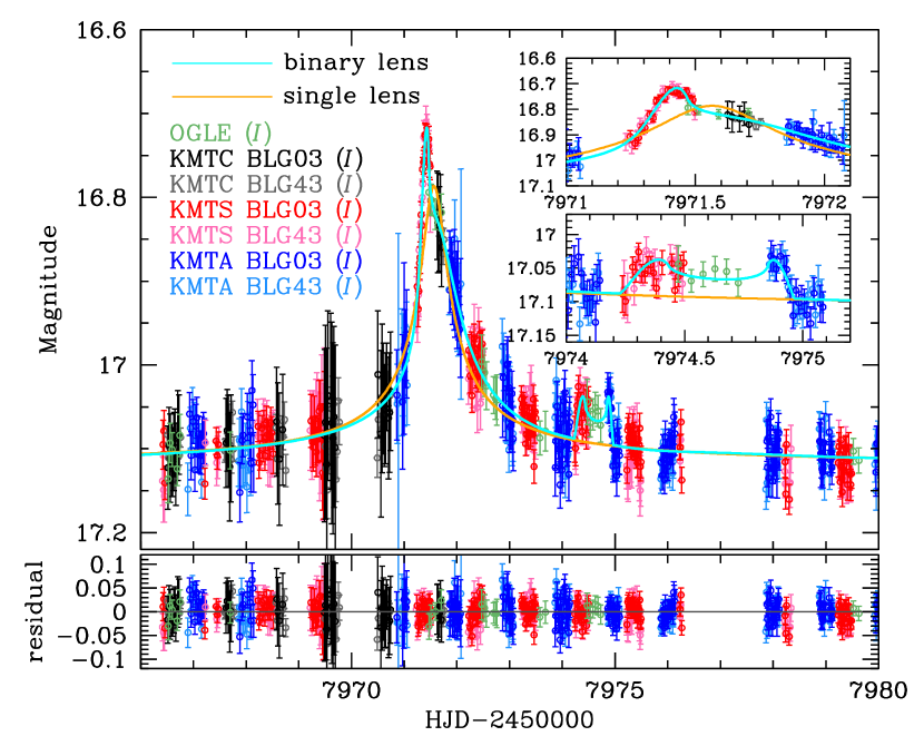
Figure 1: Light curve of OGLE-2017-BLG-1522. The upper and lower insets show the zoom of two major perturbations centered at ${\rm HJD}^{\prime}\sim 7971.4$ and $7974.6$, respectively. The cyan curve is the model curve based on the binary-lens interpretation, while the orange curve is based on the single-lens interpretation.

As presented in Figure 1, the OGLE-2017-BLG-1522 light curve shows deviations from a standard single-mass lensing curve (Paczyński, 1986). The deviations are composed of two major perturbations, one strong perturbation at ${\rm HJD}^{\prime}(={\rm HJD}-2,450,000~{}{\rm days})\sim 7971.4$ and the other weak short-term perturbation in the region between $7974<{\rm HJD}^{\prime}<7975$. The latter anomaly consists of a trough centered at ${\rm HJD}^{\prime}\sim 7974.6$ surrounded by bumps at both sides. Such a short-term anomaly is a characteristic feature that occurs when the source star crosses the small caustic induced by a low-mass companion to the primary lens. Therefore, we examine the event with the binary-lens interpretation.

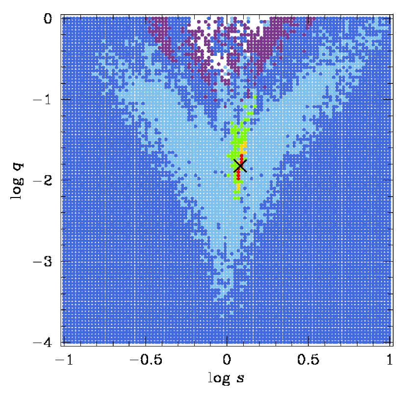
Figure 2: $\Delta\chi^{2}$ surface in $(s,q)$ space obtained from the grid search. The space is color coded by $\Delta\chi^{2}$ $<5^{2}$ (red), $<10^{2}$ (yellow), $<15^{2}$ (green), $<20^{2}$ (light blue), $<25^{2}$ (blue), and $<30^{2}$ (purple) level, respectively. The cross mark is the location of the best-fit solution.

To find the lensing parameters that describe the light curve, we adopt the parametrization and follow the procedure presented in Jung et al. (2015). We first carry out a preliminary grid search by setting $s$, $q$, and $\alpha$ as independent variables. Here $s$ and $q$ are, respectively, the projected separation (normalized to the angular Einstein radius, $\theta_{\rm E}$) and the mass ratio of the binary lens, and $\alpha$ is the trajectory angle. The grid space $(s,q,\alpha)$ is divided into $(100,100,21)$ grids and the ranges of individual variables are $-1.0<{\rm log}~{}s<1.0$, $-4.0<{\rm log}~{}q<0.0$, and $0<\alpha<2\pi$, respectively. We note that $(s,q)$ are fixed, while $\alpha$ is allowed to vary at each grid point. From this search, we identify only one local minimum. It can be seen in Figure 2, where we show the derived $\Delta\chi^{2}$ surface in the $(s,q)$ space. We then investigate the local solutions and find the global minimum by optimizing all parameters including grid variables with the Markov Chain Monte Carlo (MCMC) method.

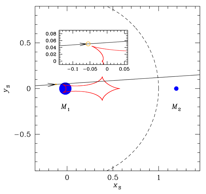
Figure 3: Geometry of the best-fit solution. The red closed curve is the caustic, the two blue dots ($M_{1}$ and $M_{2}$) are the positions of binary-lens components, and the orange circle is the size of the source. The dashed circle is the angular Einstein ring of the lens system and all lengths are scaled to its radius $\theta_{\rm E}$.

In Table 2, we list the best-fit solution determined from our modeling. The model curve of the solution is presented in Figure 1. Also shown in Figure 3 is the corresponding lensing geometry. We find that the companion-host separation is $s=1.21$ and the companion-host mass ratio is $q\sim 0.016$, implying that the companion would be in the planetary or substellar regime. In this case, the binary lens induces a single 6-sided resonant caustic near the host star (e.g., Dominik 1999). Although this caustic is resonant, it is very close to separating into a 4-sided “central caustic” (left) and a 4-sided “planetary caustic” (right), which it would do if $s$ were only slightly larger than its actual value of $s=1.21$. Specifically the transition would occur at (Erdl & Schneider, 1993)

$$s_{\rm transition}=\sqrt{(1+q^{1/3})^{3}\over 1+q}\rightarrow 1.39.$$ (2)

Hence, the cusps associated with the central-caustic wing of resonant caustic are strong, while those associated with the planetary-caustic wing are weak. The two major perturbations were generated by the source transit through the caustic. The first perturbation occurred when the source passed close to one of the central-caustic-wing cusps, while the other perturbation occurred when the source transited the caustic near one of the planetary-caustic-wing cusps.

We clearly detect finite-source effects from which the normalized source radius $\rho_{*}$ and the angular Einstein radius $\theta_{\rm E}$ is determined by

$$\theta_{\rm E}={\theta_{*}\over\rho_{*}}.$$ (3)

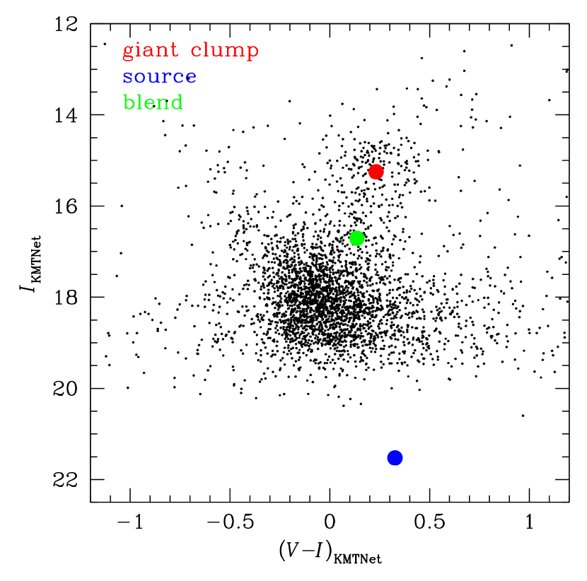
Figure 4: Position of the source star (blue dot) relative to the GC centroid (red dot) in the $(V-I,I)$ CMD of field stars around OGLE-2017-BLG-1522. The green dot is the position of blended light.

Here the angular size of the source $\theta_{*}$ is estimated from the calibrated brightness $I_{0,\rm S}$ and color $(V-I)_{0,\rm S}$ of the source. To find $(V-I,I)_{0,\rm S}$, we follow the procedure of Yoo et al. (2004). First, we build the instrumental color-magnitude diagram (CMD) using the KMTC Dophot reductions (Figure 4). Next, we estimate $(V-I,I)_{0,\rm S}$ with the equation

$$(V-I,I)_{0,\rm S}=(V-I,I)_{\rm S}-(V-I,I)_{\rm GC}+(V-I,I)_{0,\rm GC},$$ (4)

where $(V-I,I)_{\rm S}$ and $(V-I,I)_{\rm GC}$ are, respectively, the positions of the source and the giant clump (GC) centroid in the instrumental CMD, and $(V-I,I)_{0,\rm GC}=(1.06,14.34)$ is the calibrated position of the GC (Bensby et al., 2013; Nataf et al., 2013). From this, we find $(V-I,I)_{0,\rm S}=(1.15\pm 0.07,20.61\pm 0.09)$, indicating that the source is a K-type main-sequence star.

Once the source type is known, we determine $\theta_{*}$ using the $VIK$ color-color relation (Bessell & Brett, 1988) and the color-surface brightness relation (Kervella et al., 2004). The estimated angular size of the source is

$$\theta_{*}=0.390\pm 0.032~{}{\mu}{\rm as},$$ (5)

which corresponds to the angular Einstein radius

$$\theta_{\rm E}=0.065\pm 0.009~{}{\rm mas}.$$ (6)

With the measured Einstein timescale $t_{\rm E}$, the geocentric proper motion of the source relative to the lens is then

$$\mu={\theta_{\rm E}\over t_{\rm E}}=3.16\pm 0.46~{}{\rm mas~{}yr^{-1}}.$$ (7)

We note that the error in $\theta_{*}$ is derived from the uncertainty of the source brightness ($4\%$) and the color-surface brightness conversion ($7\%$). The errors of $\theta_{\rm E}$ and $\mu$ are then estimated based on $\sigma_{\theta_{*}}$ and $\sigma_{\rho_{*}}$ (see Table 2).

The Einstein radius is related to the total mass of the lens, $M_{\rm tot}$, and the distance to the lens, $D_{\rm L}$, by

$$\theta_{\rm E}=\sqrt{{\kappa}M_{\rm tot}\pi_{\rm rel}}\\ \sim 0.7{\rm mas}\left({M_{\rm tot}\over 0.7~{}M_{\odot}}\right)^{1/2}\left({8~{}{\rm kpc}\over D_{\rm S}}\right)^{1/2}\left({{1-x}\over x}\right)^{1/2},$$ (8)

where $\kappa=4G/(c^{2}{\rm AU})$, $\pi_{\rm rel}={\rm AU}(D_{\rm L}^{-1}-D_{\rm S}^{-1})$, $D_{\rm S}$ is the distance to the source, and $x=D_{\rm L}/D_{\rm S}$. Then, the derived $\theta_{\rm E}$ is significantly smaller than $\theta_{\rm E}\sim 0.7~{}{\rm mas}$ of an event caused by a stellar object with $M_{\rm tot}\sim 0.7~{}M_{\odot}$ and $x\sim 0.5$. This suggests that the event was generated by a VLM binary and/or a lens system located in the Galactic bulge very close to the source, i.e., $x\sim 1.0$.

4 Physical Parameters

The direct measurement of $M_{\rm tot}$ and $D_{\rm L}$ of the lens system requires the simultaneous detection of $\theta_{\rm E}$ and the microlens parallax $\pi_{\rm E}$, i.e.,

$$M_{\rm tot}={\theta_{\rm E}\over\kappa\pi_{\rm E}};~{}~{}~{}~{}~{}D_{\rm L}={{\rm AU}\over\pi_{\rm E}\theta_{\rm E}+\pi_{\rm S}},$$ (9)

where $\pi_{\rm S}={\rm AU}/D_{\rm S}$ is the source parallax (Gould, 1992, 2004). For OGLE-2017-BLG-1522, the angular Einstein radius is measured, but the microlens parallax cannot be measured, and thus the physical properties cannot be directly determined. Therefore, we investigate the probability distributions of physical parameters from the measured $\theta_{\rm E}$ and $t_{\rm E}$. For this, we perform a Bayesian analysis using a Galactic model based on the velocity distribution (VD), mass function (MF), and matter density profile (DP) of the Milky Way Galaxy.

In order to construct the model, we define the Cartesian coordinates in the Galactic frame so that the center of the coordinates is the Galactic center and the $x$-axis and the $z$-axis point toward the Earth and the north Galactic pole, respectively. Then, the line of sight distance $D$ of an object is related to the Galactic coordinates by

$$x=R_{\odot}-D{\rm cos}(l){\rm cos}(b),~{}y=D{\rm sin}(l){\rm cos}(b),~{}z=D{\rm sin}(b),$$ (10)

where $R_{\odot}=8~{}{\rm kpc}$ is the adopted Galactocentric distance of the Sun (Reid, 1993; Gillessen et al., 2013).

For the VD, we adopt the Han & Gould (1995) model of $f(v_{y},v_{z})=f(v_{y})f(v_{z})$ which follows a Gaussian form, i.e.,

$$f(v_{y})={1\over\sqrt{2\pi{\sigma_{y}}^{2}}}{\rm exp}\left[-{(v_{y}-\bar{v}_{y})^{2}\over 2{\sigma_{y}}^{2}}\right]$$ (11)

and a similar form for $f(v_{z})$. Here $\bar{v}$ and $\sigma$ denote the mean and dispersion of the velocity component, respectively. Following Han & Gould (1995), we use $(\bar{v}_{z,\rm bulge},\bar{v}_{z,\rm disk})=(0,0)~{}{\rm km}~{}{\rm s}^{-1}$ and $(\sigma_{z,\rm bulge},\sigma_{z,\rm disk})=(100,20)~{}{\rm km}~{}{\rm s}^{-1}$ for the $z$-direction and $(\bar{v}_{y,\rm bulge},\bar{v}_{y,\rm disk})=(0,220)~{}{\rm km}~{}{\rm s}^{-1}$ and $(\sigma_{y,\rm bulge},\sigma_{y,\rm disk})=(100,30)~{}{\rm km}~{}{\rm s}^{-1}$ for the $y$-direction. For a given set of the projected velocity of the lens $\mathbb{v}_{\rm L}$, the source $\mathbb{v}_{\rm S}$, and the observer $\mathbb{v}_{\rm o}$, the transverse velocity of the lens with respect to the source $\mathbb{v}$ is then given by

$$\mathbb{v}=\mathbb{v}_{\rm L}-\left[\mathbb{v}_{\rm S}{D_{\rm L}\over D_{\rm S}}+\mathbb{v}_{\rm o}{{D_{\rm S}-D_{\rm L}}\over D_{\rm S}}\right].$$ (12)

The projected velocity of the observer $\mathbb{v}_{\rm o}$ is estimated by converting the heliocentric Earth’s velocity at the peak time of the event, $\mathbb{v}_{\rm E}=(v_{\rm E,\rm E},v_{\rm E,\rm N})=(21.07,-1.75)~{}{\rm km}~{}{\rm s}^{-1}$, to the Galactic frame. In this procedure, we also consider the peculiar and circular motion of the Sun with respect to a local standard of rest, i.e., $\mathbb{v}_{\odot}=\mathbb{v}_{\odot,\rm pec}+\mathbb{v}_{\odot,\rm cir}=(12,7)+(220,0)~{}{\rm km}~{}{\rm s}^{-1}$.

For the MF, we separately consider the bulge and the disk lens populations. We model the bulge population by adopting the log-normal initial mass function (IMF: Chabrier, 2003), while we model the disk population by adopting the log-normal present-day mass function (PDMF: Chabrier, 2003). In both functions, the lower mass limit is set to $0.01~{}M_{\odot}$. We note that we do not consider stellar remnants, since planets orbiting a star in the phase of asymptotic giant branch or planetary nebular would be hard to survive, and thus the probability to find planets orbiting a remnant would be extremely low (e.g., Kilic et al., 2009).

For the DP, we use a triaxial profile for the bulge and a double exponential profile for the disk. In the case of bulge profile, we adopt the refined Han & Gould (2003) model for which the profile follows the Dwek et al. (1995) model and the density is normalized by the star count results of Holtzman et al. (1998). The disk profile is modeled by the two (thin and thick disk) exponential disks of the form

$$\rho_{r,z}=\rho(R_{\odot},0)e^{R_{\odot}/{h_{R}}}{\rm exp}\left(-{r\over h_{R}}-{{z+z_{\odot}}\over h_{Z}}\right),$$ (13)

where $r=(x^{2}+y^{2})^{1/2}$, $z_{\odot}$ is the offset of the Sun from the Galactic plane, and $h_{R}$ and $h_{Z}$ are the radial and vertical scale length, respectively. We adopt $z_{\odot}=25~{}{\rm pc}$, $(h_{R},h_{Z})_{\rm thin}=(2600,300)~{}{\rm pc}$, $(h_{R},h_{Z})_{\rm thick}=(3600,900)~{}{\rm pc}$, and the normalization factor $f=\rho_{\rm thick}(R_{\odot},0)/\rho_{\rm thin}(R_{\odot},0)=0.12$ from Jurić et al. (2008), where they construct the profile using stellar objects detected by the Sloan Digital Sky Survey (SDSS: York et al., 2000). Finally, we normalize the number density to $\rho(R_{\odot},0)=0.05~{}M_{\odot}~{}{\rm pc}^{-3}$ by following the disk density of solar neighborhood estimated by Han & Gould (2003).

With the adopted models of VD, MF, and DP, we generate microlensing events from the Monte Carlo simulation and then investigate the probability distributions of the host mass $M_{1}$ and lens distance using the measured $\theta_{\rm E}$ and $t_{\rm E}$ as a prior . In Figure 5, we show the posterior probabilities of $M_{1}$ (upper panel) and $D_{\rm L}$ (lower panel) derived from our Bayesian analysis. The median value of the mass and the distance with $68\%$ $(1\sigma)$ confidence intervals are

$$M_{1}={0.045}_{-0.024}^{+0.076}~{}M_{\odot},~{}~{}~{}~{}~{}D_{\rm L}={7.49}_{-0.88}^{+0.91}~{}{\rm kpc},$$ (14)

respectively. The estimated host star corresponds to a brown dwarf. The median value of the lens distance implies that both the lens and the source are likely to be located in the Galactic bulge. These consequently indicate that the extraordinarily small value of $\theta_{\rm E}$ is due to the combination of the small lens mass and the lens location close to the source.

From the measured $q$, the companion mass is determined by

$$M_{2}=qM_{1}=0.75_{-0.40}^{+1.26}~{}M_{\rm J},$$ (15)

which roughly corresponds to the Jupiter mass planet. The physical companion-host projected separation is

$$a_{\bot}=s{D_{\rm L}}{\theta_{\rm E}}=0.59_{-0.11}^{+0.12}~{}{\rm AU}.$$ (16)

By adopting that the snow line scales with the host mass (Kennedy & Kenyon, 2008), we estimate the snow line of the lens system by $a_{sl}=2.7~{}{\rm AU}(M/M_{\odot})\sim 0.12~{}{\rm AU}$, indicating that the giant plant is placed beyond the snow line.

5 Discussion

We found a planetary candidate around a probable brown dwarf host located in the Galactic bulge. The probability that the host is a brown dwarf (i.e., $M_{1}<0.08~{}M_{\odot}$) is $\sim$ 76% (see Figure 5). The light curve perturbations were clearly identified by the OGLE survey and continuously covered by the KMTNet observations despite the relatively short event timescale $(t_{\rm E}\sim 7.5~{}{\rm days})$, which enabled the unambiguous characterization of the lens system. This proves the capability of current microlensing experiments. In Figure 6, we compare the mass distribution of the lens to those of known exoplanets. From this, we find that this event could be the first binary that closes the gap between terrestrial and jovian mass companions in the brown-dwarf host region. We also find that MOA-2013-BLG-605 could have similar properties to our results (Sumi et al., 2016). However, it not only suffers from large uncertainties ($3\sim 21~{}M_{\oplus}$ for the companion and $0.03\sim 0.2~{}M_{\odot}$ for the host) due to the severe degeneracy in the parallax measurement but also favors the terrestrial planet interpretation. It is worth noting that the analysis of a large sample of short-timescale binary events found by Mróz et al. (2017) can bring additional information on the population of planetary-mass companions to brown dwarf hosts.

Up to now, several brown dwarfs hosting giant planet companions have been discovered. However, their large mass ratios $(q\gtrsim 0.1)$ between the host and the companion would suggest that they are formed as binary systems either by the dynamical interaction in unstable molecular clouds (Bate, 2009, 2012) or by the turbulent fragmentation of molecular cloud cores (Padoan & Nordlund, 2004). This implies that the companions could be considered as substellar objects rather than planets (Chabrier et al., 2014). By contrast, the low mass ratio of this event $(q\sim 0.016)$, combined with recent reports of the massive disks $(\gtrsim M_{\rm J})$ around young brown dwarfs (Hervey et al., 2012; André et al., 2012; Palau et al., 2014), suggest that the planetary companion of the event may be formed by planet formation mechanisms. Therefore, OGLE-2017-BLG-1522Lb could be the first giant planet orbiting around a brown-dwarf host having a planetary mass ratio.

It would therefore be of considerable interest to make a definitive determination of whether the host is a brown dwarf or a star. Considering that the measured relative source motion is $\mu\sim 3~{}{\rm mas~{}yr^{-1}}$, the source will be separated from the lens about $\gtrsim 30~{}{\rm mas}$ at first light of the upcoming next generation ($D\sim 30$m class) telescopes. Then, the source and the lens could be resolved with these telescopes because their resolution in $H$ band will be $\theta=14(D/30{\rm m})^{-1}~{}{\rm mas}$. Hence, at first light for any of these telescopes, the source and lens will be separated by well over $1$ FWHM. If the host is a star rather than a brown dwarf, $M>0.08~{}M_{\odot}$, then $M_{H,{\rm host}}\lesssim 9$ and $\pi_{\rm rel}<6.4~{}{\mu}{\rm as}$, i.e., $D_{\rm L}\sim 8~{}{\rm kpc}$. The $H$ band magnitude of the host is then $H_{{\rm host}}\lesssim 23.5$ which should be easily visible in AO images. As a result, the nature of the host (star or brown dwarf) can be unambiguously resolved at that time.

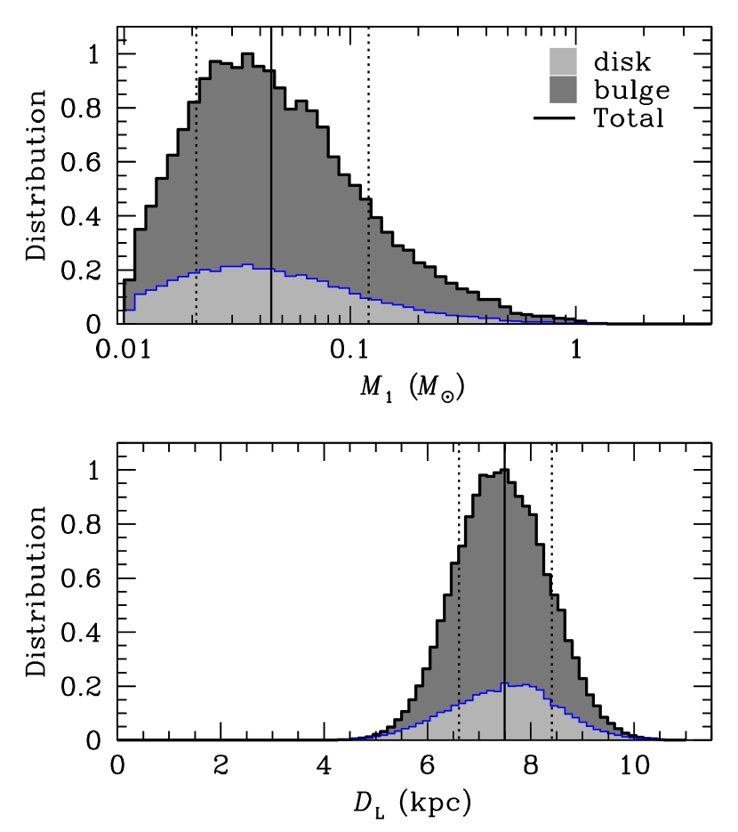
Figure 5: Probability distributions of the host mass (upper panel) and lens distance (lower panel) derived from the Bayesian analysis. The grey and darkgrey distributions are those derived from the disk and bulge Galactic models, respectively. In each panel, the solid line represents the median value and the two dotted lines represent the confidence intervals estimated based on the lower and upper boundaries encompassing the $68\%$ $(1\sigma)$ range of the distribution.

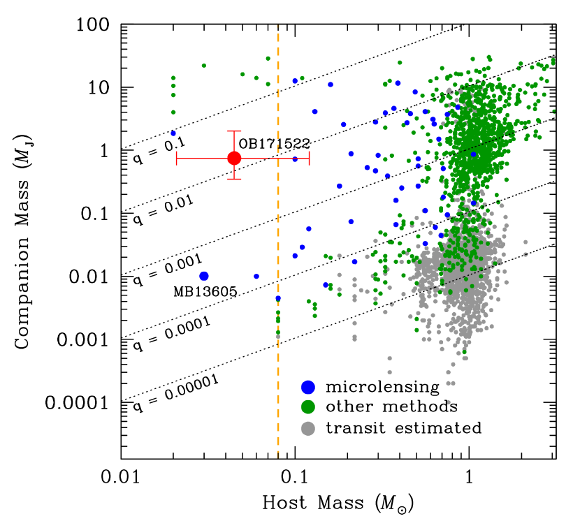
Figure 6: Mass distribution of known exoplanets. The red dot is OGLE-2017-BLG-1522. The planets discovered by microlensing method are marked by blue dots, while those found by other methods are marked by green dots. For transiting systems for which companion masses are not directly determined, we estimate the companion mass using the forecasting model of Chen & Kipping (2017) (grey dots). The yellow vertical dashed line represents the conventional star/brown-dwarf boundary. The values are acquired from http://exoplanetarchive.ipac.caltech.edu.

Table 1: Error Correction Parameters

Observatory	Number	$k$	$\sigma_{\rm min}$ (mag)
OGLE $(I)$	11365	1.672	0.002
KMTC BLG03 $(I)$	1336	1.153	0.000
KMTC BLG43 $(I)$	1639	1.438	0.000
KMTS BLG03 $(I)$	2323	1.268	0.000
KMTS BLG43 $(I)$	2173	1.389	0.000
KMTA BLG03 $(I)$	1787	1.679	0.000
KMTA BLG43 $(I)$	1818	1.506	0.000

Table 2: Lensing Parameters

Parameters	Values
$\chi^{2}$/dof	21009.3/22434
$t_{0}$ (${\rm HJD^{\prime}}$)	7971.80 $\pm$ 0.01
$u_{0}$ ($10^{-2}$)	5.39 $\pm$ 0.34
$t_{\rm E}$ (days)	7.53 $\pm$ 0.28
$s$	1.21 $\pm$ 0.01
$q$ ($10^{-2}$)	1.59 $\pm$ 0.16
$\alpha$ (rad)	6.22 $\pm$ 0.01
$\rho_{\ast}$ ($10^{-2}$)	0.60 $\pm$ 0.07
$f_{\rm S}$	0.035 $\pm$ 0.002
$f_{\rm B}$	2.221 $\pm$ 0.002

Note. — ${\rm HJD}^{\prime}={\rm HJD}-2,450,000~{}{\rm days}$

References

- Alard & Lupton (1998) Alard, C., & Lupton, Robert H. 1998, ApJ, 503, 325
- Albrow et al. (2009) Albrow, M. D., Horne, K., Bramich, D. M., et al. 2009, MNRAS, 397, 2099
- André et al. (2012) André, P., Ward-Thompson, D., & Greaves, J. 2012, Sci, 337, 69
- Apai et al. (2005) Apai, D., Pascucci, I., Bouwman, J., et al. 2005, Sci, 310, 834
- Bate (2009) Bate, M. R. 2009, MNRAS, 392, 590
- Bate (2012) Bate, M. R. 2012, MNRAS, 419, 3115
- Bensby et al. (2013) Bensby, T., Yee, J. C., Feltzing, S., et al. 2013, A&A, 549, 147
- Bessell & Brett (1988) Bessell, M. S., & Brett, J. M. 1988, PASP, 100, 1134
- Boss (2006) Boss, A. P. 2006, ApJ, 643, 501
- Chabrier (2003) Chabrier, G. 2003, PASP, 115, 763
- Chabrier et al. (2014) Chabrier, G., Johansen, A., Janson, M., & Rafikov, R. 2014, in Protostars and Planets VI, Giant Planet and Brown Dwarf Formation, ed. H. Beuther et al. (Tucson, AZ: Univ. Arizona Press), 619
- Chauvin et al. (2004) Chauvin, G., Lagrange, A. M., Dumas, C., et al. 2004, A&A, 425, L29
- Chen & Kipping (2017) Chen, J., & Kipping, D. 2017, ApJ, 834, 17
- Dominik (1999) Dominik, M. 1999, A&A, 349, 108
- Dwek et al. (1995) Dwek, E., Arendt, R. G., Hauser, M. G., et al. 1995, ApJ, 445, 716
- Erdl & Schneider (1993) Erdl, H., & Schneider, P. 1993, A&A, 268, 453
- Furusawa et al. (2013) Furusawa, K., Udalski, A., Sumi, T., et al. 2013, ApJ, 779, 91
- Gauza et al. (2015) Gauza, B., Béjar, V. J. S., Pérez-Garrido, A., et al. 2015, ApJ, 804, 96
- Gillessen et al. (2013) Gillessen, S., Eisenhauer, F., Fritz, T. K., et al. 2013, in IAU Symp. 289, Advancing the Physics of Cosmic Distances, ed. R. de Grijs (Cambridge: Cambridge Univ. Press), 29
- Gould (1992) Gould, A. 1992, ApJ, 392, 442
- Gould (2004) Gould, A. 2004, ApJ, 606, 319
- Han & Gould (1995) Han, C., & Gould, A. 1995, ApJ, 447, 53
- Han & Gould (2003) Han, C., & Gould, A. 2003, ApJ, 592, 172
- Han et al. (2013) Han, C., Jung, Y. K., Udalski, A., et al. 2013, ApJ, 778, 38
- Hervey et al. (2012) Harvey, P. M., Henning, Th., Liu, Y., et al. 2012, ApJ, 755, 67
- Holtzman et al. (1998) Holtzman, J. A., Watson, A. M., Baum, W. A., et al. 1998, AJ, 115, 1946
- Ida & Lin (2004) Ida, S., & Lin, D. N. C. 2004, ApJ, 616, 567
- Joergens & Muller (2007) Joergens, V., & Muller, A. 2007, ApJ, 666, L113
- Jung et al. (2015) Jung, Y. K., Udalski, A., Sumi, T., et al. 2015, ApJ, 798, 123
- Jurić et al. (2008) Jurić, M., Ivezić, Z., Brooks, A., et al. 2008, ApJ, 673, 864
- Kennedy et al. (2006) Kennedy, G. M., Kenyon, S. J., & Bromley, B. C. 2006, ApJ, 650, L139
- Kennedy & Kenyon (2008) Kennedy, G. M., & Kenyon, S. J. 2008, ApJ, 673, 502
- Kervella et al. (2004) Kervella P., Thévenin F., Di Folco E., Ségransan D., 2004, A&A, 426, 297
- Kilic et al. (2009) Kilic, M., Gould, A., & Koester, D. 2009, ApJ, 705, 1219
- Kim et al. (2016) Kim, S.-L., Lee, C.-U., Park, B.-G., et al. 2016, JKAS, 49, 37
- Laughlin et al. (2004) Laughlin, G., Bodenheimer, P., & Adams, F. C. 2004, ApJ, 612, L73
- Luhman (2012) Luhman, K. L. 2012, ARA&A, 50, 65
- Mayor & Queloz (1995) Mayor, M., & Queloz, D. 1995, Nature, 378, 355
- Mróz et al. (2017) Mróz, P., Udalski, A., Skowron, J. et al. 2017 Nature, 548, 183
- Nagakane et al. (2017) Nagakane, M., Sumi, T., Koshimoto, N., et al. 2017, AJ, 154,35
- Nataf et al. (2013) Nataf, D. M., Gould, A., Fouqué, P., et al. 2013, ApJ, 769, 88
- Paczyński (1986) Paczyński, B. 1986, ApJ, 304, 1
- Padoan & Nordlund (2004) Padoan, P., & Nordlund, A. 2004, ApJ, 617, 559
- Palau et al. (2014) Palau, A., Zapata, L. A., Rodríguez, L. F., et al. 2014, MNRAS, 444, 833
- Pepe et al. (2011) Pepe, F., Lovis, C., & Ségransan, D. 2011, A&A, 534, A58
- Reid (1993) Reid, M. J. 1993, ARA&A, 31, 345
- Ricker et al. (2014) Ricker, G. R., Winn, J. N., Vanderspek, R., et al. 2014, JATIS, 1, 014003
- Riaz et al. (2012) Riaz, B., Lodieu, N., Goodwin, S., Stamatellos, D., & Thompson, M. 2012, MNRAS, 420, 2497
- Shvartzvald et al. (2017) Shvartzvald, Y., Yee, J. C., Calchi Novati, S., et al. 2017, ApJ, 840, L3
- Skowron et al. (2015) Skowron, J., Shin, I.-G., Udalski, A., et al. 2015, ApJ, 804, 33
- Skowron et al. (2016) Skowron, J., Udalski, A., Kozłowski, S., et al. 2016, Acta Astron., 66, 1
- Stone et al. (2016) Stone, J. M., Skemer, A. J., Kratter, K. M., et al. 2016, ApJ, 818, L12
- Street et al. (2013) Street, R. A., Choi, J.-Y., Tsapras, Y., et al. 2013, ApJ, 763, 67
- Tenenbaum et al. (2014) Tenenbaum, P., Jenkins, J. M., Seader, S., et al. 2014, ApJS, 211, 6
- Todorov et al. (2010) Todorov, K., Luhman, K. L., & Mcleod, K. K. 2010, ApJ, 714, L84
- Spiegel et al. (2011) Spiegel, D. S., Burrows, A., & Milsom, J. A. 2011, ApJ, 727, 57
- Sumi et al. (2016) Sumi, T., Udalski, A., Bennett, D. P., et al. 2016 ApJ, 825, 112
- Udalski (2003) Udalski, A. 2003, Acta Astron., 53, 291
- Udalski et al. (2015) Udalski, A., Szymański, M. K., & Szymański, G. 2015, Acta Astron, 65, 1
- Wolszczan & Frail (1992) Wolszczan, A., & Frail, D. A. 1992, Nature, 355, 145
- Yee et al. (2012) Yee, J. C., Shvartzvald, Y., Gal-Yam, A., et al. 2012, ApJ, 755, 102
- Yoo et al. (2004) Yoo, J., DePoy, D. L., Gal-Yam, A., et al. 2004, ApJ, 603, 139
- York et al. (2000) York, D. G., Adelman, J., Anderson, J. E., et al. 2000, AJ, 120, 1579