Deletion in abstract Voronoi diagrams in expected linear time and related problems

Abstract

Updating an abstract Voronoi diagram after deletion of one site in linear time has been a well-known open problem; similarly, for concrete Voronoi diagrams of non-point sites. In this paper, we present an expected linear-time algorithm to update an abstract Voronoi diagram after deletion of one site. We introduce the concept of a Voronoi-like diagram, a relaxed version of an abstract Voronoi construct that has a structure similar to an ordinary Voronoi diagram, without, however, being one. We formalize the concept, and prove that it is robust under insertion, therefore, enabling its use in incremental constructions. The time-complexity analysis of the resulting simple randomized incremental construction is non-standard, and interesting in its own right, because the intermediate Voronoi-like structures are order-dependent. We further extend the approach to compute the following structures in expected linear time: the order-$(k{+}1)$ subdivision within an order-$k$ Voronoi region, and the farthest abstract Voronoi diagram after the order of its regions at infinity is known.

Keywords:

abstract Voronoi diagram; linear-time algorithm; randomized incremental construction; site-deletion; higher-order Voronoi diagram; farthest Voronoi diagram.

1 Introduction

The Voronoi diagram of a set $S$ of $n$ simple geometric objects, called sites, is a versatile and well-known geometric partitioning structure, which reveals proximity information for the input sites. Classic variants include the nearest-neighbor, the farthest-site, and the order-$k$ Voronoi diagram of the set $S$. Abstract Voronoi diagrams offer a unifying framework to many concrete and fundamental instances. Voronoi diagrams have been well-investigated and optimal construction algorithms exist in many cases. For more information see, e.g., the book of Aurenhammer et al. [2] and also [18] for a wealth of applications.

For certain Voronoi diagrams with a tree structure, linear-time construction algorithms have been well-known to exist, see e.g., [1, 7, 14, 8]. The first linear-time technique was introduced by Aggarwal et al. [1] for the Voronoi diagram of points in convex position, given the order of the points along their convex hull. The same technique can be used to derive linear-time algorithms for other fundamental problems: (1) updating a Voronoi diagram of points after deletion of one site in time linear to the number of Voronoi neighbors of the deleted site; (2) computing the order-$(k{+}1)$ subdivision within an order-$k$ Voronoi region; (3) computing the farthest Voronoi diagram of point-sites in linear time, after computing their convex hull. A much simpler randomized approach for the same problems was introduced by Chew [7]. The medial axis of a simple polygon is another well-known problem to admit a linear-time construction, as shown by Chin et al. [8].

Surprisingly, no linear-time constructions have been known for any of the problems (1)-(3) for Voronoi diagrams concerning non-point sites, and similarly for abstract Voronoi diagrams. Under restrictions, Klein and Lingas [14] adapted the linear-time approach of [1] to the abstract framework, showing that a Hamiltonian abstract Voronoi diagram can be computed in linear time, given the order of Voronoi regions along an unbounded simple curve, which visits each region exactly once and can intersect each bisector only once. This construction has been extended recently to include some forest structures [4], under similar restrictions, where no region can have multiple faces within a domain enclosed by a curve, and each bisector can intersect this domain in one component.

In this paper we consider the fundamental problem of site-deletion in abstract Voronoi diagrams and provide a simple expected linear-time technique to achieve this task. We work in the framework of abstract Voronoi diagrams so that we can simultaneously address all the concrete instances that fall under their umbrella. After deletion, we extend the randomized linear-time technique to the remaining problems: (cfr. 2) computing the order-$(k{+}1)$ subdivision within an order-$k$ abstract Voronoi region; and (cfr. 3) computing the farthest abstract Voronoi diagram, after the order of its faces at infinity is known. To the best of our knowledge, no deterministic linear-time technique is yet known for these problems. In the process, we define a Voronoi-like diagram, a relaxed Voronoi structure, which is interesting in its own right. Voronoi-like regions are supersets of real Voronoi regions, and their boundaries correspond to simple monotone paths in the arrangement of the underlying bisector system (see Definition 1). We prove correctness and uniqueness of this structure and use it to derive a very simple technique to address the above problems in expected linear time.

An earlier attempt towards a linear-time construction for the farthest-segment Voronoi diagram appeared in [11], following a different geometric formulation for segments, which however, does not extend to the abstract setting. A preliminary version of this paper regarding site deletion in abstract Voronoi diagrams appeared in [10]. In three dimensions, site-deletion in Delaunay triangulations of point-sites, as inspired by the randomized approach of Chew [7], has been considered in [6].

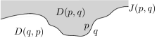
Figure 1: A bisector $J(p,q)$ and its two dominance regions; $D(p,q)$ is shown shaded.

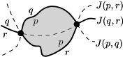
Figure 2: The Voronoi diagram of 3 sites, the underlying bisector system in dashed lines, and $\mbox{VR}(p,\{p,q,r\})$ shaded.

Abstract Voronoi diagrams (AVDs).

These diagrams were introduced by Klein [12]. Instead of sites and distance measures, they are defined in terms of bisecting curves that satisfy some simple combinatorial properties. Given a set $S$ of $n$ abstract sites, the bisector $J(p,q)$ of two sites $p,q\in S$ is an unbounded Jordan curve, homeomorphic to a line, that divides the plane into two open domains: the dominance region of $p$, $D(p,q)$ (having label $p$), and the dominance region of $q$, $D(q,p)$ (having label $q$), see Fig. 2. The Voronoi region of $p$ is

$$\mbox{VR}(p,S)=\bigcap_{q\in S\setminus\{p\}}D(p,q).$$

The (nearest-neighbor) Voronoi diagram of $S$ is

$$\mathcal{V}(S)=\mathbb{R}^{2}\setminus\bigcup_{p\in S}\mbox{VR}(p,S).$$

Following the traditional model of AVDs (see e.g. [12, 3, 4]) the bisector system is assumed to satisfy the following axioms, for every subset $S^{\prime}\subseteq S$:

1. Each Voronoi region $\mbox{VR}(p,S^{\prime})$ is non-empty and path-connected.

2. Each point in the plane belongs to the closure of a Voronoi region $\mbox{VR}(p,S^{\prime})$.

3. Each bisector $J(p,q)$ is an unbounded curve, which after stereographic projection to the sphere can be completed to a closed Jordan curve through the north pole.

4. Any two bisectors $J(p,q)$ and $J(r,t)$ intersect transversally and in a finite number of points. (It is possible to relax this axiom, see [13]).

The abstract Voronoi diagram $\mathcal{V}(S)$ is a plane graph of structural complexity $O(n)$ whose regions are simply connected. It can be computed in time $O(n\log n)$, both randomized [15] and deterministic [12].

To update $\mathcal{V}(S)$ after deleting one site $s\in S$, we need to compute $\mathcal{V}(S\setminus\{s\})$ within $\mbox{VR}(s,S)$. This diagram is a tree, if $\mbox{VR}(s,S)$ is bounded, and a forest otherwise. However, its regions can be disconnected, and one region may consist of multiple faces. In fact, site-occurrences along $\partial\mbox{VR}(s,S)$ form a Davenport-Schinzel sequence of order 2. Disconnected regions introduce severe complications and constitute a major difficulty, which differentiates the problem from its counterpart on point sites. For example, let $S^{\prime}\subset S\setminus\{s\}$; the diagram $\mathcal{V}(S^{\prime})\cap\mbox{VR}(s,S^{\prime}\cup\{s\})$ may contain faces that do not even appear in $\mathcal{V}(S\setminus\{s\})\cap\mbox{VR}(s,S)$, and conversely, an arbitrary sub-sequence of arcs on $\partial\mbox{VR}(s,S)$ need not be related to any Voronoi diagram. At a first sight, a linear-time algorithm may even seem infeasible.

Our results.

In this paper we formalize the concept of a Voronoi-like diagram, a relaxed Voronoi structure defined as a graph (a tree or forest) in the arrangement of the underlying bisector system, and prove that it is well-defined and unique. This structure provides the tool we need to deal with disconnected Voronoi regions, and thus, address the site-deletion problem efficiently. Given a Voronoi-like diagram, we define an insertion operation and prove its correctness. This makes a simple randomized incremental construction possible. The time-analysis of the randomized algorithm is non-standard because the intermediate Voronoi-like structures are order-dependent. We give a technique, which partitions the permutations of length $i$ into manageable groups of $i$ permutations each, and show that the time complexity per group is $O(i)$, deriving that each insertion step can be performed in expected $O(1)$ time. This technique may be independently useful in deriving expectation in order-dependent cases. In this paper we focus on site-deletion, computing $\mathcal{V}(S\setminus\{s\})\cap\mbox{VR}(s,S)$ in expected time $O(|\partial\mbox{VR}(s,S)|)$, i.e., in expected time linear in the number of Voronoi neighbors of the deleted site. We also extend the approach to address problems (2) and (3) for the order-$k$ and the farthest abstract Voronoi diagram respectively. The sequence of the faces at infinity of the latter diagram can be computed in time $O(n\log n)$.

Examples of concrete diagrams that fall under the AVD umbrella and thus they benefit from our approach include: disjoint line segments and disjoint convex polygons of constant size in the $L_{p}$ norms, or under the Hausdorff metric; point-sites in any convex distance metric or the Karlsruhe metric; additively weighted points that have non-enclosing circles; power diagrams with non-enclosing circles.

2 Preliminaries

Let $S$ be a set of $n$ abstract sites (a set of indices) that define an admissible system of bisectors $\mathcal{J}=\{J(p,q):p\neq q\in S\}$. $\mathcal{J}$ fulfills axioms (A1)–(A4) for every $S^{\prime}\subseteq S$.

Bisectors in $\mathcal{J}$ that have a site $p$ in common are called $p$-related or simply related. Any two related bisectors can intersect at most twice [12, Lemma 3.5.2.5]. When two related bisectors $J(p,q)$ and $J(p,r)$ intersect, bisector $J(q,r)$ also intersects with them at the same point(s), and these points are the Voronoi vertices of the diagram $\mathcal{V}(\{p,q,r\})$. The Voronoi diagram of three sites $\mathcal{V}(\{p,q,r\})$ may have one or two (or none) Voronoi vertices, see Fig. 2. The set of all $p$-related bisectors that involve sites in $S^{\prime}\subseteq S$ is denoted $\mathcal{J}_{p,S^{\prime}}=\{J(p,q)\,|\,q\in S^{\prime},q\neq p\}$.

Let $\mbox{VR}(s,S)$ be the Voronoi region of a site $s\in S$. Although $\mbox{VR}(s,S)$ is simply connected, the sites in $S\setminus\{s\}$ that appear along the boundary $\partial\mbox{VR}(s,S)$ may repeat, forming a Davenport-Schinzel sequence of order 2. This is because $s$-related bisectors can intersect at most twice, and thus, [21, Theorem 5.7] applies. This is a fundamental difference from the classic case of point-sites in the Euclidean plane, where bisectors are straight-lines, therefore they intersect once, and no site repetition can occur along $\partial\mbox{VR}(s,S)$.

Suppose we delete the site $s\in S$ from $\mathcal{V}(S)$. To update the Voronoi diagram after the deletion of $s$, we need to compute $\mathcal{V}(S\setminus\{s\})$ within the Voronoi region $\mbox{VR}(s,S)$, i.e., compute $\mathcal{V}(S\setminus\{s\})\cap\mbox{VR}(s,S)$. We first characterize the structure of this diagram in the following lemma. An alternative proof and characterization can be derived from the order-$k$ counterpart [5], however, this proof appeared later, after the preliminary version of this paper [10].

Figure 3: $\mathcal{V}(S\setminus\{s\})\cap\mbox{VR}(s,S)$ in red; $\partial\mbox{VR}(s,S)$ is shown in bold black.

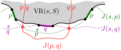
Figure 4: $\mbox{VR}(p,S\setminus\{s\})\cap\mbox{VR}(s,S)$ cannot be connected because of $J(p,q)$.

Lemma 1.

$\mathcal{V}(S\setminus\{s\})\cap\mbox{VR}(s,S)$ is a forest, having exactly one face for each Voronoi edge of $\partial\mbox{VR}(s,S)$. Its leaves are the Voronoi vertices of $\partial\mbox{VR}(s,S)$, and points at infinity if $\mbox{VR}(s,S)$ is unbounded (see Fig. 4). If $\mbox{VR}(s,S)$ is bounded then $\mathcal{V}(S\setminus\{s\})\cap\mbox{VR}(s,S)$ is a tree.

Proof.

Every face in $\mathcal{V}(S\setminus\{s\})\cap\mbox{VR}(s,S)$ must touch the boundary $\partial\mbox{VR}(s,S)$ because Voronoi regions are non-empty and connected; this implies that the diagram is a forest. Every Voronoi edge $e\subseteq J(s,p)$ on $\partial\mbox{VR}(s,S)$ must be entirely in $\mbox{VR}(p,S\setminus\{s\})$. Thus, no leaf can lie in the interior of a Voronoi edge of $\partial\mbox{VR}(s,S)$. On the other hand, each Voronoi vertex of $\partial\mbox{VR}(s,S)$ must be a leaf of the diagram as its incident edges are induced by different sites.

Now we show that no two edges of $\partial\mbox{VR}(s,S)$ can be incident to the same face of $\mathcal{V}(S\setminus\{s\})\cap\mbox{VR}(s,S)$. Consider two edges on $\partial\mbox{VR}(s,S)$ induced by the same site $p\in S\setminus\{s\}$. Then there exists an edge between them, induced by a site $q\neq p$, such that the bisector $J(s,q)$ has exactly two intersections with $J(p,s)$ as shown in Fig. 4. The bisector $J(p,q)$ intersects with them at the same two points. Since the bisector system is admissible, and thus $\mbox{VR}(p,\{s,p,q\})$ is connected, $J(p,q)$ connects these endpoints through $D(p,s)\cap D(q,s)$ as shown in Fig. 4, thus, $J(p,q)\cap\mbox{VR}(s,\{s,p,q\})$ consists of two unbounded connected components. This implies that $D(p,q)\cap\mbox{VR}(s,S)$ must have two disjoint faces, each of which is incident to exactly one of the two edges of $p$. Thus, $\mbox{VR}(p,S\setminus\{s\})\cap\mbox{VR}(s,S)$ cannot be connected and the two edges of $p$ must be incident to different faces of $\mathcal{V}(S\setminus\{s\})\cap\mbox{VR}(s,S)$.

If $\mbox{VR}(s,S)$ is unbounded, two consecutive edges of $\partial\mbox{VR}(s,S)$ can extend to infinity, in which case there is at least one edge of $\mathcal{V}(S\setminus\{s\})\cap\mbox{VR}(s,S)$ extending to infinity between them; thus, leaves can be points at infinity. If $\mbox{VR}(s,S)$ is bounded, all leaves of $\mathcal{V}(S\setminus\{s\})\cap\mbox{VR}(s,S)$ must lie on $\partial\mbox{VR}(s,S)$. Since no face is incident to more than one edge of $\partial\mbox{VR}(s,S)$, in this case $\mathcal{V}(S\setminus\{s\})\cap\mbox{VR}(s,S)$ cannot be disconnected, and thus is a tree. ∎

Let $\Gamma$ be a closed Jordan curve in the plane large enough to enclose all the intersections of bisectors in $\mathcal{J}$, and such that each bisector intersects $\Gamma$ exactly twice and transversally. To avoid dealing with infinity, and without any loss of generality, we restrict all computations within $\Gamma$. The curve $\Gamma$ can be interpreted as $J(p,s_{\infty})$, for all $p\in S$, where $s_{\infty}$ is an additional site at infinity. Let $D_{\Gamma}$ denote the portion of the plane enclosed by $\Gamma$. $\mbox{VR}(s,S)\cap D_{\Gamma}$ is the domain of our computation. Fig. 5 illustrates possible cases of the computation domain.

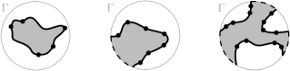
Figure 5: The domain of computation $\mbox{VR}(s,S)\cap D_{\Gamma}$ (shaded).

We first make some observations regarding an admissible bisector system, which we use as tools in the proofs throughout this paper. Let $C_{p}$ be a cycle of $p$-related bisectors in the arrangement of bisectors $\mathcal{J}\cup\Gamma$. If the label $p$ appears on the outside of the cycle for every edge in $C_{p}$, then $C_{p}$ is called $p$-inverse, see Fig. 6(a). If the label $p$ appears only inside $C_{p}$ then $C_{p}$ is called a $p$-cycle, see Fig. 6(b). Recall that $\Gamma$ can be considered a $p$-related bisector, for all sites $p\in S$, where the label $p$ is in the interior of $\Gamma$. Thus, a $p$-cycle may contain pieces of $\Gamma$, whereas a $p$-inverse cycle cannot contain any such piece.

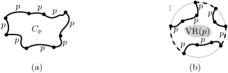
Figure 6: (a) A $p$-inverse cycle. (b) A $p$-cycle.

Lemma 2.

In an admissible bisector system there is no $p$-inverse cycle.

Proof.

Suppose a $p$-inverse cycle exists in the admissible bisector system. Let $C_{p}$ denote a minimal such cycle, where no $p$-related bisector may intersect the interior of $C_{p}$ and let $D_{p}$ denote the interior of $C_{p}$. Such a minimal cycle must exist because if a bisector $J(p,q)$ intersects $D_{p}$, then it defines another (smaller) $p$-inverse cycle that is contained in $C_{p}\cup D_{p}$ and whose interior is not intersected by $J(p,q)$. Let $S^{\prime}\subseteq S$ denote the set of sites that define the edges of $C_{p}$. Considering $S^{\prime}$, the farthest Voronoi region of $p$ is $\mbox{FVR}(p,S^{\prime})=\bigcap_{q\in S^{\prime}\setminus\{p\}}D(q,p)$. But by its definition, $D_{p}$ must be identical to one face of $\mbox{FVR}(p,S^{\prime})$. Since farthest Voronoi regions must be unbounded [17, 3], we derive a contradiction. ∎

The following transitivity lemma is a consequence of transitivity of dominance regions [3, Lemma 2] and the fact that bisectors $J(p,q),J(q,r)$, $J(p,r)$ intersect at the same point(s). Let $\overline{X}$ denote the closure of a region $X$.

Lemma 3.

Let $z\in\mathbb{R}^{2}$ and $p,q,r\in S$. If $z\in D(p,q)$ and $z\in\overline{D(q,r)}$, then $z\in D(p,r)$.

We make a general position assumption that no three $p$-related bisectors intersect at the same point. This implies that Voronoi vertices have degree 3.

3 Problem formulation, definitions and properties

Let $\mathscr{S}$ denote the sequence of Voronoi edges bounding the Voronoi region $\mbox{VR}(s,S)$ within the domain $D_{\Gamma}$, i.e., $\mathscr{S}=\partial\mbox{VR}(s,S)\cap D_{\Gamma}$. We consider $\mathscr{S}$ as a cyclically ordered set of arcs, where each arc is a portion of an $s$-related bisector defining a Voronoi edge along $\partial\mbox{VR}(s,S)$. A single site in $S\setminus\{s\}$ may induce several arcs in $\mathscr{S}$. For any arc $\alpha\in\mathscr{S}$, let $s_{\alpha}$ denote the site in $S$ such that $\alpha\subseteq J(s,s_{\alpha})$.

We can interpret the arcs in $\mathscr{S}$ as sites that induce a Voronoi diagram $\mathcal{V}(\mathscr{S})$ such that $\mathcal{V}(\mathscr{S})=\mathcal{V}(S\setminus\{s\})\cap\mbox{VR}(s,S)\cap D_{\Gamma}$, see Fig. 7. By Lemma 1, each face of $\mathcal{V}(\mathscr{S})$ is incident to exactly one arc in $\mathscr{S}$. Thus, the face of $\mathcal{V}(\mathscr{S})$ incident to an arc $\alpha\in\mathscr{S}$ can be considered its Voronoi region $\text{VR}(\alpha,\mathscr{S})$. Then $\mathcal{V}(\mathscr{S})$ can be regarded as the diagram derived by the Voronoi regions of the arcs in $\mathscr{S}$.

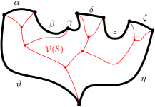
Figure 7: Illustration of $\mathscr{S}=\partial\mbox{VR}(s,S)$ in bold (black) and $\mathcal{V}(\mathscr{S})$ in red; $\mathscr{S}=(\alpha,\beta,\gamma,\delta,\varepsilon,\zeta,\eta,\vartheta)$.

The arrangement of a bisector set $\mathcal{J}^{\prime}\subseteq\mathcal{J}$ is denoted by $\mathcal{A}(\mathcal{J}^{\prime})$. A path $P$ in the arrangement $\mathcal{A}(\mathcal{J}^{\prime})$ is a connected sequence of alternating edges and vertices in this arrangement. An arc $\alpha$ of $P$ (denoted as $\alpha\in P$) is a maximally connected collection of consecutive edges and vertices of the arrangement along $P$, which belong to the same bisector. The common endpoint of two consecutive arcs of $P$ is a vertex of $P$. An arc of $P$ is also called an edge. Two consecutive arcs in a path $P$ are pieces of different bisectors.

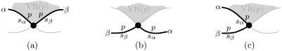
Figure 8: (a) Arcs $\alpha,\beta$ fulfill the $p$-monotone path condition; they do not fulfill it (b) and (c).

Definition 1.

A path in the arrangement of $p$-related bisectors $\mathcal{J}_{p,S^{\prime}}$, $S^{\prime}\subseteq S$, is called $p$-monotone if any two consecutive arcs $\alpha,\beta$ along this path, where $\alpha\subseteq J(p,s_{\alpha})$ and $\beta\subseteq J(p,s_{\beta})$, coincide locally (within a neighborhood of their common endpoint) with Voronoi edges of $\partial\mbox{VR}(p,\{p,s_{\alpha},s_{\beta}\})$ that are incident to this common endpoint (see Fig. 8 and Fig. 9).

Definition 2.

The $p$-envelope (or simply envelope) of $\mathcal{J}_{p,S^{\prime}}$ is $\text{env}(\mathcal{J}_{p,S^{\prime}})=\partial\mbox{VR}(p,S^{\prime}\cup\{p\})$ (see Fig. 9(a)).

The arrangement of the bisectors in $\mathcal{J}_{p,S^{\prime}}$ may consist of several connected components. We can unify these connected components by including $\Gamma$ in the bisector system. Then, $\text{env}(\mathcal{J}_{p,S^{\prime}}\cup\Gamma)$ is a single closed $p$-monotone path, which contains all the connected components of $\text{env}(\mathcal{J}_{p,S^{\prime}})$ interleaved by arcs of $\Gamma$. $\mbox{VR}(s,S)$ and in particular to a subset $\mathscr{S}^{\prime}$ of its Voronoi edges.

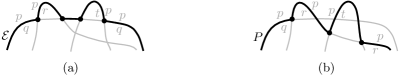
Figure 9: (a) The envelope $\mathcal{E}=\text{env}(\mathcal{J}_{p,\{q,r,t\}})$. (b) A $p$-monotone path $P$ in $\mathcal{J}_{p,\{q,r,t\}}$.

Definition 3.

Consider $\mathscr{S}^{\prime}\subseteq\mathscr{S}$ and let $S^{\prime}=\{s_{\alpha}\in S\,|\,\alpha\in\mathscr{S}^{\prime}\}$ be the corresponding set of its sites. A boundary curve $\mathcal{P}$ for $\mathscr{S}^{\prime}$ is a closed $s$-monotone path in the arrangement of $s$-related bisectors $\mathcal{J}_{s,S^{\prime}}\cup\Gamma$ such that all arcs in $\mathscr{S}^{\prime}$ are contained in $\mathcal{P}$. Let $D_{\mathcal{P}}$ denote the domain of $\mathcal{P}$, which is the part of the plane enclosed by $\mathcal{P}$. Let $S_{\mathcal{P}}=S^{\prime}$.

A set $\mathscr{S}^{\prime}\subset\mathscr{S}$ can admit several different boundary curves; one such boundary curve is its $s$-envelope $\mathcal{E}=env(\mathscr{S}^{\prime})=\text{env}(\mathcal{J}_{s,S^{\prime}}\cup\Gamma)$. The set $\mathscr{S}$ can admit only one boundary curve, which is its $s$-envelope $env(\mathscr{S})=\partial(\mbox{VR}(s,S)\cap D_{\Gamma})$. Fig. 10 illustrates a boundary curve for a subset of arcs from Fig. 7.

A boundary curve $\mathcal{P}$ consists of pieces of $s$-bisectors called boundary arcs, and pieces of $\Gamma$, called $\Gamma$-arcs. $\Gamma$-arcs correspond to openings of the domain $D_{\mathcal{P}}$ to infinity. Among the boundary arcs, those containing an arc of $\mathscr{S}^{\prime}$ are called original and others are called auxiliary arcs. Original boundary arcs in $\mathcal{P}$ are expanded versions of the arcs in $\mathscr{S}$. To distinguish them, we call the elements of $\mathscr{S}$ core arcs and use an ^∗ in their notation. We denote by $|\mathcal{P}|$ the number of boundary arcs in $\mathcal{P}$. Fig. 10 illustrates a boundary curve $\mathcal{P}$ on $\mathscr{S}^{\prime}\subseteq\mathscr{S}$ consisting of five original arcs, one auxiliary arc ($\beta^{\prime}$) and one $\Gamma$-arc ($g$); the core arcs are illustrated in bold; the set $\mathscr{S}$ is shown in Fig. 7.

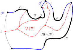
Figure 10: A boundary curve $\mathcal{P}$ on $\mathscr{S}^{\prime}\subseteq\mathscr{S}$, where $\mathscr{S}^{\prime}$ is shown in bold, and its Voronoi-like diagram $\mathcal{V}_{l}(\mathcal{P})$ shown in thin red. The gray arc $g$ is a $\Gamma$-arc, and the blue arc $\beta^{\prime}$ is an auxiliary arc; the remaining arcs are original. The set $\mathscr{S}$ is shown in Fig. 7.

We now define the Voronoi-like diagram of a boundary curve $\mathcal{P}$ on $\mathscr{S}^{\prime}\subseteq\mathscr{S}$, where $S^{\prime}=\{s_{\alpha}\in S\,|\,\alpha\in\mathscr{S}^{\prime}\}$ is the corresponding set of sites. Let $\mathcal{J}(S^{\prime})\subseteq\mathcal{J}$ be the system of bisectors related to $S^{\prime}$, i.e., $\mathcal{J}(S^{\prime})=\{J(p,q)\in\mathcal{J}\,|\,p,q\in S^{\prime}\}$.

Definition 4.

Given a boundary curve $\mathcal{P}$ on $\mathscr{S}^{\prime}\subseteq\mathscr{S}$, the Voronoi-like diagram of $\mathcal{P}$ is a plane graph $\mathcal{V}_{l}(\mathcal{P})$ on the arrangement of the bisector system $\mathcal{J}(S^{\prime})$ inducing a subdivision of the domain $D_{\mathcal{P}}$ as follows (see Fig. 10):

1. for each boundary arc $\alpha\in\mathcal{P}$, there is exactly one distinct face $R(\alpha,\mathcal{P})$, whose boundary is an $s_{\alpha}$-monotone path in $\mathcal{J}_{s_{\alpha},S^{\prime}}\cup\Gamma$, plus arc $\alpha$;

2. the faces cover the domain $D_{\mathcal{P}}$: $\bigcup_{\alpha\in{\mathcal{P}\setminus\Gamma}}\overline{R(\alpha,\mathcal{P})}=\overline{D_{\mathcal{P}}}$.

Voronoi-like regions in $\mathcal{V}_{l}(\mathcal{P})$ are related to the real Voronoi regions as supersets as we show in the following lemma. Let $\mathcal{V}(\mathcal{E})=\mathcal{V}(S^{\prime})\cap D_{\mathcal{E}}$ be the Voronoi diagram of the $s$-envelope $\mathcal{E}$ of $\mathscr{S}^{\prime}$. In $\mathcal{V}(\mathcal{E})$ any face incident to a boundary arc $\alpha\in\mathcal{E}$ can be regarded as its Voronoi region $\mbox{VR}(\alpha,\mathcal{E})$. For an original arc $\alpha\in\mathcal{P}$ there is an original arc $\tilde{\alpha}\in\mathcal{E}$ and a core arc $\alpha^{*}\in\mathscr{S}$ such that $\alpha\supseteq\tilde{\alpha}\supseteq\alpha^{*}$.

Lemma 4.

Let $\alpha\in\mathcal{P}$ be a boundary arc such that $\tilde{\alpha}\subseteq\alpha$ appears on the $s$-envelope $\mathcal{E}$. Then, $R(\alpha,\mathcal{P})\supseteq\mbox{VR}(\tilde{\alpha},\mathcal{E})$. Further, if $\alpha$ is original, then $R(\alpha,\mathcal{P})\supseteq\mbox{VR}(\tilde{\alpha},\mathcal{E})\supseteq\mbox{VR}(\alpha^{*},\mathscr{S})$.

Proof.

By the definition of a Voronoi region, no piece of a bisector $J(s_{\alpha},\cdot)$ can appear in the interior of a Voronoi region in $\mathcal{V}(S^{\prime})\cap D_{\mathcal{E}}$. Thus no piece of $J(s_{\alpha},\cdot)$ can appear in $\mbox{VR}(\tilde{\alpha},\mathcal{E})$, for any $\tilde{\alpha}\in\mathcal{E}$. Since $\alpha\supseteq\tilde{\alpha}$, by the definition of a Voronoi-like region it follows that $R(\alpha,\mathcal{P})\supseteq\mbox{VR}(\tilde{\alpha},\mathcal{E})$. For an original arc $\alpha$, since $S^{\prime}\subseteq S$, by the monotonicity property of Voronoi regions, we also have $\mbox{VR}(\tilde{\alpha},\mathcal{E})\supseteq\mbox{VR}(\alpha^{*},\mathscr{S})$. ∎

In Fig. 10 the Voronoi-like region $R(\eta,\mathcal{P})$ is a superset of its corresponding Voronoi region $\mbox{VR}(\eta^{*},\mathscr{S})$ of $\mathcal{V}(\mathscr{S})$ in Fig. 7; similarly $R(\alpha,\mathcal{P})\supseteq\mbox{VR}(\alpha^{*},\mathscr{S})$.

As a corollary to the superset property of Lemma 4, the adjacencies of the real Voronoi diagram $\mathcal{V}(\mathcal{E})$ are preserved in $\mathcal{V}_{l}(\mathcal{P})$, for all the original arcs. As a result, $\mathcal{V}_{l}(\mathcal{E})$ must coincide with the real Voronoi diagram $\mathcal{V}(\mathcal{E})=\mathcal{V}(S^{\prime})\cap D_{\mathcal{E}}$.

Corollary 1.

$\mathcal{V}_{l}(\mathcal{E})=\mathcal{V}(\mathcal{E})=\mathcal{V}(S^{\prime})\cap D_{\mathcal{E}}$ for the $s$-envelope $\mathcal{E}$ of $\mathscr{S}^{\prime}\subseteq\mathscr{S}$.

Proof.

Consider two arcs $\alpha\neq\beta$ of $\mathcal{E}$. Suppose $\mbox{VR}(\alpha,\mathcal{E})$ is adjacent to $\mbox{VR}(\beta,\mathcal{E})$. Since by Lemma 4, $R(\alpha,\mathcal{E})\supseteq\mbox{VR}(\alpha,\mathcal{E})$ and $R(\beta,\mathcal{E})\supseteq\mbox{VR}(\beta,\mathcal{E})$, it follows that $R(\alpha,\mathcal{E})$ must be adjacent to $R(\beta,\mathcal{E})$. This implies that the regions in $\mathcal{V}_{l}(\mathcal{E})$ have the same adjacencies as in $\mathcal{V}(\mathcal{E})$. Lemma 4 also implies that there can be no additional adjacencies; thus, $\mathcal{V}_{l}(\mathcal{E})=\mathcal{V}(\mathcal{E})$. ∎

In the remaining section we give basic properties of Voronoi-like regions involving their interaction with the bisectors in $\mathcal{J}$, which we use to derive correctness and establish that the Voronoi-like diagram is well-defined.

3.1 Properties of Voronoi-like regions

The following property establishes that a Voronoi-like region $R(\alpha,\mathcal{P})$ can never be intersected by $J(s,s_{\alpha})$.

Lemma 5.

For any arc $\alpha\in\mathcal{P}$, $R(\alpha,\mathcal{P})\subseteq D(s,s_{\alpha})$.

Proof.

The contrary would yield a forbidden $s_{\alpha}$-inverse cycle defined by a component of $J(s,s_{\alpha})\cap R(\alpha,\mathcal{P})$ and the incident portion of $\partial R(\alpha,\mathcal{P})$. ∎

Lemma 6.

For a boundary curve $\mathcal{P}$, its domain $\overline{D_{\mathcal{P}}}$ may not contain a $p$-cycle formed by the bisectors of $\mathcal{J}(S_{\mathcal{P}})\cup\Gamma$, for any site $p\in S_{\mathcal{P}}$.

Proof.

Let $p\in S_{\mathcal{P}}$. Any original arc of $p$ in $\mathcal{P}$ is bounding $\mbox{VR}(p,S_{\mathcal{P}}\cup\{s\})$, thus, it must have a portion within the interior of $\mbox{VR}(p,S_{\mathcal{P}})$ in $\mathcal{V}(S_{\mathcal{P}})$. Hence, $\mbox{VR}(p,S_{\mathcal{P}})$ must have some non-empty portion outside the closure of $D_{\mathcal{P}}$. However, $\mbox{VR}(p,S_{\mathcal{P}})\cap D_{\Gamma}$ must be enclosed within any $p$-cycle of $\mathcal{J}(S_{\mathcal{P}})\cup\Gamma$, by its definition. Thus, no such $p$-cycle can be contained in $\overline{D_{\mathcal{P}}}$. ∎

Next, we give a key property of a Voronoi-like region, which we call the cut property, see Fig. 11. Suppose bisector $J(s_{\alpha},s_{\beta})$ intersects the Voronoi-like region $R(\alpha,\mathcal{P})$. Let $e$ be a connected component of $J(s_{\alpha},s_{\beta})\cap R(\alpha,\mathcal{P})$ and let $R_{e}(\alpha)$ denote the portion of region $R(\alpha,\mathcal{P})$ that is cut out by $e$ as shown in Fig. 11. More precisely $R_{e}(\alpha)$ is defined as follows. If $e$ does not intersect $\alpha$, then $R_{e}(\alpha)$ is the portion of the region at the opposite side of $e$ as $\alpha$ (case (a), see Fig. 11(a)). Otherwise, let $\tilde{\beta}$ be the component of $J(s,s_{\beta})\cap R(\alpha,\mathcal{P})$ incident to $e$ and $\alpha$, and let $R_{e}(\alpha)$ be the portion of $R(\alpha,\mathcal{P})$ that contains $\tilde{\beta}$ (cases (b) and (d) in Fig. 11). If there is another component of $J(s_{\alpha},s_{\beta})\cap R(\alpha,\mathcal{P})$ incident to $\alpha$, let $R_{e}(\alpha)$ be the portion of $R(\alpha,\mathcal{P})$ between the two components (case (c), see Fig. 11(c)). Note that if $\beta\in\mathcal{P}$ then cases (c) and (d) cannot appear since related bisectors can only intersect twice.

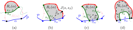
Figure 11: Illustrations for Lemma 7. The shaded region $R_{e}(\alpha)$ lies in $D(s_{\beta},s_{\alpha})$.

Lemma 7.

Suppose bisector $J(s_{\alpha},s_{\beta})$ appears within $R(\alpha,\mathcal{P})$ (see Fig. 11). For any connected component $e$ of $J(s_{\alpha},s_{\beta})\cap R(\alpha,\mathcal{P})$, it holds $R_{e}(\alpha)\subseteq D(s_{\beta},s_{\alpha})$. Thus, if $e$ does not intersect $\alpha$, the label $s_{\alpha}$ must appear on the same side of $e$ as $\alpha$.

Note that $\partial R_{e}(\alpha)$ may contain $\Gamma$-arcs.

Proof.

Let $e$ be an arbitrary component of $J(s_{\alpha},s_{\beta})\cap R(\alpha,\mathcal{P})$. Suppose for the sake of contradiction that $R_{e}(\alpha)\not\subseteq D(s_{\beta},s_{\alpha})$. Then $J(s_{\beta},s_{\alpha})$ must intersect the interior of $R_{e}(\alpha)$ with a component $e^{\prime}$ of $J(s_{\beta},s_{\alpha})\cap R(\alpha,\mathcal{P})$, which is different from $e$. Among any such component, let $e^{\prime}$ be the first one following $e$ along $J(s_{\beta},s_{\alpha})$. Since $e^{\prime}$ cannot intersect $e$, nor can it intersect $\tilde{\beta}$, it follows that $e^{\prime}$ must create an $s_{\alpha}$-cycle with $\partial R_{e}(\alpha)$, contradicting Lemma 6. ∎

Lemma 7 implies that any components of $J(s_{\alpha},s_{\beta})\cap R(\alpha,\mathcal{P})$ must appear sequentially along $\partial R(\alpha,\mathcal{P})$. In addition, if any such component exists, $J(s,s_{\beta})$ must also intersect the domain $D_{\mathcal{P}}$ with a component that is missing from $\mathcal{P}$. We use this fact to establish that $\mathcal{V}_{l}(\mathcal{P})$ is unique in the following theorem whose proof is deferred to Section 5.

Theorem 1.

Given a boundary curve $\mathcal{P}$ of $\mathscr{S}^{\prime}\subseteq\mathscr{S}$, $\mathcal{V}_{l}(\mathcal{P})$ is unique, assuming it exists.

The complexity of $\mathcal{V}_{l}(\mathcal{P})$ is $O(|\mathcal{P}|)$ as it is a planar graph with exactly one face per boundary arc and vertices of degree 3 (or 1).

4 Insertion in a Voronoi-like diagram

Consider a boundary curve $\mathcal{P}$ on a set of core arcs $\mathscr{S}^{\prime}\subset\mathscr{S}$ and its Voronoi-like diagram $\mathcal{V}_{l}(\mathcal{P})$. Let $\beta^{*}$ be a core arc in $\mathscr{S}\setminus\mathscr{S}^{\prime}$. Since $\beta^{*}$ is a core arc, it must be entirely contained in the domain $D_{\mathcal{P}}$. We define an insertion operation $\oplus$, which inserts a core arc $\beta^{*}$ in $\mathcal{P}$, and derives the boundary curve $\mathcal{P}_{\beta}=\mathcal{P}\oplus\beta^{*}$ and $\mathcal{V}_{l}(\mathcal{P}_{\beta})=\mathcal{V}_{l}(\mathcal{P})\oplus\beta^{*}$.

Given $\mathcal{P}$ and $\beta^{*}$, let the original arc $\beta\supseteq\beta^{*}$ be the connected component of $J(s,s_{\beta})\cap\overline{D_{\mathcal{P}}}$ that contains $\beta^{*}$, see Fig. 12. $\mathcal{P}_{\beta}$ is the boundary curve derived from $\mathcal{P}$ by substituting its portion between the endpoints of $\beta$, with $\beta$ itself. We say that $\mathcal{P}_{\beta}$ is derived from $\mathcal{P}$ by inserting the core arc $\beta^{*}$, or equivalently, by inserting the original arc $\beta$.

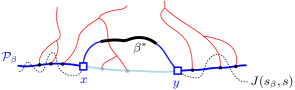
Figure 12: $\mathcal{P}_{\beta}=\mathcal{P}\oplus\beta$, core arc $\beta^{*}$ is bold, black. Endpoints of $\beta$ are $x,y$.

The insertion operation $\oplus$ performs the following tasks algorithmically: (1) inserts the core arc $\beta^{*}$ in $\mathcal{P}$, deriving $\mathcal{P}_{\beta}=\mathcal{P}\oplus\beta^{*}=\mathcal{P}\oplus\beta$; (2) computes a merge curve $J(\beta)$, which defines the boundary of $R(\beta,\mathcal{P}_{\beta})$; and (3) updates $\mathcal{V}_{l}(\mathcal{P})$ to derive $\mathcal{V}_{l}(\mathcal{P}_{\beta})=\mathcal{V}_{l}(\mathcal{P})\oplus\beta$. Fig. 13 enumerates all possible cases in task 1 and it is summarized in the following observation.

Observation 1.

All possible cases of inserting arc $\beta^{*}\subseteq\beta$ in $\mathcal{P}$ are as follows (see Fig. 13).

1. Arc $\beta$ straddles the endpoint of two consecutive boundary arcs; no arcs in $\mathcal{P}$ are deleted.

2. Auxiliary arcs in $\mathcal{P}$ are deleted by $\beta$; their regions are also deleted from $\mathcal{V}_{l}(\mathcal{P}_{\beta})$.

3. An arc $\alpha\in\mathcal{P}$ is split into two arcs by $\beta$; $R(\alpha,\mathcal{P})$ will also be split.

4. A $\Gamma$-arc is split in two by $\beta$; $\mathcal{V}_{l}(\mathcal{P}_{\beta})$ may switch from being a tree to being a forest.

5. A $\Gamma$-arc is deleted or shrunk by inserting $\beta$. $\mathcal{V}_{l}(\mathcal{P}_{\beta})$ may become a tree.

6. $\mathcal{P}$ already contains a boundary arc $\bar{\beta}\supseteq\beta^{*}$; then $\beta=\bar{\beta}$ and $\mathcal{P}_{\beta}=\mathcal{P}$.

$\mathcal{P}_{\beta}$ may contain fewer, the same number, or even one additional auxiliary arc compared to $\mathcal{P}$.

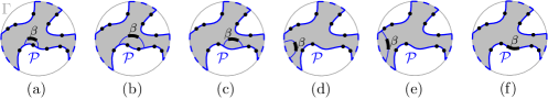
Figure 13: Insertion cases for an arc $\beta$.

Given $\mathcal{V}_{l}(\mathcal{P})$ and arc $\beta$, we define a merge curve $J(\beta)$, which delimits the boundary of $R(\beta,\mathcal{P}_{\beta})$. We define $J(\beta)$ algorithmically, starting at an endpoint of $\beta$, and tracing $s_{\beta}$-related bisectors within the faces of $\mathcal{V}_{l}(\mathcal{P})$, refer to Fig. 16. We prove that $J(\beta)$ is an $s_{\beta}$-monotone path that connects the endpoints of $\beta$. Let $x,y$ denote the endpoints of $\beta$, where $x\beta y$ appear in counterclockwise order. We assume a counterclockwise traversal of $\mathcal{P}$.

Definition 5.

Given $\mathcal{V}_{l}(\mathcal{P})$ and arc $\beta\subseteq J(s,s_{\beta})$, the merge curve $J(\beta)$ is a path $(v_{1},\dots,v_{m})$ in the arrangement of $s_{\beta}$-related bisectors, $\mathcal{J}_{s_{\beta},S_{\mathcal{P}}}\cup\Gamma$, connecting the endpoints of $\beta$, $v_{1}=x$ and $v_{m}=y$. Each edge $e_{i}=(v_{i},v_{i+1})$ is an arc of a bisector $J(s_{\beta},\cdot)$, called a bisector edge, or an arc on $\Gamma$. We assume a clockwise ordering of $J(\beta)$. For $i=1$: if $x\in J(s_{\beta},s_{\alpha})$, then $e_{1}\subseteq J(s_{\beta},s_{\alpha})$; if $x\in\Gamma$, then $e_{1}\subseteq\Gamma$. Given $v_{i}$, vertex $v_{i+1}$ and edge $e_{i+1}$ are defined as follows:

1. If $e_{i}\subseteq J(s_{\beta},s_{\alpha})$, let $v_{i+1}$ be the other endpoint of the component $J(s_{\beta},s_{\alpha})\cap R(\alpha,\mathcal{P})$ incident to $v_{i}$. If $v_{i+1}\in J(s_{\beta},\cdot)\cap J(s_{\beta},s_{\alpha})$, then $e_{i+1}\subseteq J(s_{\beta},\cdot)$. If $v_{i+1}\in\Gamma$, then $e_{i+1}\subseteq\Gamma$. (In Fig. 16, see $e_{i}=e^{\prime},v_{i}=z,v_{i+1}=z^{\prime}$.)

2. If $e_{i}\subseteq\Gamma$, let $g$ be the $\Gamma$-arc in $\mathcal{P}$ incident to $v_{i}$. Let $e_{i+1}\subseteq J(s_{\beta},s_{\gamma})$, where $R(\gamma,\mathcal{P})$ is the first region, incident to $g$ clockwise from $v_{i}$ such that $J(s_{\beta},s_{\gamma})$ intersects $g\cap\overline{R(\gamma,\mathcal{P})}$; let $v_{i+1}$ be this intersection point. (In Fig. 16, see $v_{i}=v$ and $v_{i+1}=w$.)

The following theorem shows that $J(\beta)$ forms an $s_{\beta}$-monotone path joining the endpoints of $\beta$. We defer its proof to the end of this section.

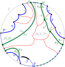
Figure 14: The merge curve $J(\beta)$ (thick, green) on $\mathcal{V}_{l}(\mathcal{P})$ (thin, red).

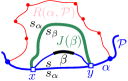
Figure 15: If $\beta$ splits $\alpha$, $J(\beta)\subset R(\alpha,\mathcal{P})$ would yield a forbidden $s_{\alpha}$-inverse cycle.

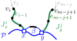
Figure 16: $J_{x}^{i}$ and $J_{y}^{j}$ in Section 4.1.

Theorem 2.

The merge curve $J(\beta)$ is a unique $s_{\beta}$-monotone path in the arrangement of $s_{\beta}$-related bisectors $\mathcal{A}(\mathcal{J}_{s_{\beta},S_{\mathcal{P}}}\cup\Gamma)$ connecting the endpoints of $\beta$. If arc $\beta$ splits a single arc $\alpha\in\mathcal{P}$ (case (c), Observation 1) then $J(\beta)$ must intersect $R(\alpha,\mathcal{P})$ in two different components, $e_{1},e_{m-1}\subseteq J(s_{\alpha},s_{\beta})$. $J(\beta)$ can intersect any other region in $\mathcal{V}_{l}(\mathcal{P})$ at most once. $J(\beta)$ cannot intersect the region of any arc in $\mathcal{P}\setminus\mathcal{P}_{\beta}$, which gets deleted by the insertion of $\beta$, nor can it intersect arc $\beta$ in its interior.

Let $T(\beta)$ denote the portion of $\mathcal{V}_{l}(\mathcal{P})$ enclosed by $J(\beta)$. ${\mathcal{V}_{l}(\mathcal{P})\oplus\beta}$ is obtained from $\mathcal{V}_{l}(\mathcal{P})$ by deleting $T(\beta)$ and substituting it by $J(\beta)$, i.e., ${\mathcal{V}_{l}(\mathcal{P})\oplus\beta}=\big{(}\mathcal{V}_{l}(\mathcal{P})\setminus T(\beta)\big{)}\cup J(\beta)$.

Theorem 3.

${\mathcal{V}_{l}(\mathcal{P})\oplus\beta}$ is the Voronoi-like diagram $\mathcal{V}_{l}(\mathcal{P}_{\beta})$.

Proof.

By construction, ${\mathcal{V}_{l}(\mathcal{P})\oplus\beta}$ induces a subdivision of the domain $D_{\mathcal{P}_{\beta}}$. Let $R(\alpha)$ denote the face of ${\mathcal{V}_{l}(\mathcal{P})\oplus\beta}$ incident to a boundary arc $\alpha\in\mathcal{P}_{\beta}$. By Theorem 2, $J(\beta)$, and thus, $\partial R(\beta)\setminus\beta$, is an $s_{\beta}$-monotone path connecting the endpoints of $\beta$. For any arc $\alpha\in\mathcal{P}$ such that $J(\beta)$ passes through $R(\alpha,\mathcal{P})$, the boundary of the updated face in ${\mathcal{V}_{l}(\mathcal{P})\oplus\beta}$ remains an $s_{\alpha}$-monotone path, by the definition of $J(\beta)$. Thus, $\partial R(\alpha)\setminus\alpha$ is an $s_{\alpha}$-monotone path for any region $R(\alpha)$ in ${\mathcal{V}_{l}(\mathcal{P})\oplus\beta}$, satisfying the first requirement of Definition 4.

Since $J(\beta)$ can enter any region in $\mathcal{V}_{l}(\mathcal{P})$ at most once (except case (c), Observation 1)) it cannot cut out a face that may remain in the interior of $D_{\mathcal{P}}$. In addition, $J(\beta)$ cannot pass through any region of an arc in $\mathcal{P}\setminus\mathcal{P}_{\beta}$, thus, such a region must be enclosed by $J(\beta)$ and will be deleted. Hence, any face of ${\mathcal{V}_{l}(\mathcal{P})\oplus\beta}$ must be incident to a boundary arc of $\mathcal{P}_{\beta}$, satisfying also the second requirement of Definition 4. Since, by Theorem 1, the Voronoi-like diagram of a boundary curve is unique, it follows that ${\mathcal{V}_{l}(\mathcal{P})\oplus\beta}=\mathcal{V}_{l}(\mathcal{P}_{\beta})$. ∎

The tracing of the merge curve $J(\beta)$ within $\mathcal{V}_{l}(\mathcal{P})$, given the endpoints of $\beta$, can be done in linear time similarly to tracing such a curve in any ordinary Voronoi diagram, see, e.g., [2, Ch. 7.5.3]. This is correct as a result of the cut property of Lemma 7. When $J(\beta)$ enters a region $R(\gamma,\mathcal{P})$ at a point $v_{i}$, we can determine $v_{i+1}$ by scanning $\partial R(\gamma,\mathcal{P})$ counterclockwise sequentially until we encounter the first intersection with $J(s_{\beta},s_{\gamma})$. Lemma 7 assures that no intersection of $J(s_{\beta},s_{\gamma})$ with $\partial R(\gamma,\mathcal{P})$ between $v_{i}$ and $v_{i+1}$ is possible, such as the one shown in Fig. 17. Thus, we can state the following fact.

Lemma 8.

Let $e_{i}=(v_{i},v_{i+1})$ be an edge of $J(\beta)$ in $R(\gamma,\mathcal{P})$. Given $v_{i}$, we can determine $v_{i+1}$ by sequentially scanning $\partial R(\gamma,\mathcal{P})$ counterclockwise from $v_{i}$ (i.e., away from $\gamma$) until the first intersection of $J(s_{\beta},s_{\gamma})$ with $\partial R(\gamma,\mathcal{P})$ which determines $v_{i+1}$.

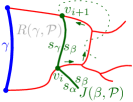
Figure 17: Impossible configuration of $J(s_{\beta},s_{\gamma})$. Scanning $\partial R(\gamma,\mathcal{P})$ from $v_{i}$ counterclockwise, Lemma 7 assures that $v_{i+1}$ is the first encountered intersection of $J(s_{\beta},s_{\gamma})$ with $\partial R(\gamma,\mathcal{P})$.

Special care is required in Observation 1, cases (c), (d), (e), to identify the first edge of $J(\beta)$ because $\beta$ does not overlap any feature of $\mathcal{V}_{l}(\mathcal{P})$. To handle them we need some parameters as defined below.

Let $\tilde{\mathcal{P}}$ denote the finer version of $\mathcal{P}$ derived by intersecting its $\Gamma$-arcs with $\mathcal{V}_{l}(\mathcal{P})$, i.e., partitioning the $\Gamma$-arcs of $\mathcal{P}$ into finer pieces by the incident faces of $\mathcal{V}_{l}(\mathcal{P})$. Since the complexity of $\mathcal{V}_{l}(\mathcal{P})$ is $O(|\mathcal{P}|)$, it follows that $|\tilde{\mathcal{P}}|$ is also $O(|\mathcal{P}|)$.

Definition 6.

Let $\alpha$ and $\gamma$ denote the original arcs preceding and following $\beta$ on $\mathcal{P}_{\beta}$. We assume a counterclockwise traversal of $\mathcal{P}$ and $\mathcal{P}_{\beta}$.

1. Let $d_{1}(\beta,\mathcal{P}_{\beta})$ denote the number of auxiliary arcs that appear on $\mathcal{P}_{\beta}$ from $\alpha$ to $\beta$ (or equivalently from $\beta$ to $\gamma$).

2. Let $d_{2}(\beta,\mathcal{P}_{\beta})$ denote the number of auxiliary arcs that appear on $\mathcal{P}$ between the endpoints of $\beta$, which get deleted by the insertion of $\beta$.

3. In case (c) of Observation 1, where $\beta$ splits an arc $\omega$ in two arcs $(\omega_{1},\omega_{2})$, let $r(\beta,\mathcal{P}_{\beta})=\min\{|\partial R(\omega_{1},\mathcal{P}_{\beta})|,|\partial R(\omega_{2},\mathcal{P}_{\beta})|\}$; otherwise, let $r(\beta,\mathcal{P}_{\beta})=0$.

4. In case (d) of Observation 1, where $\beta$ splits a $\Gamma$-arc, let $\tilde{d}(\beta,\mathcal{P}_{\beta})$ denote the number of fine $\Gamma$-arcs on $\tilde{\mathcal{P}}_{\beta}$ from $\alpha$ to $\beta$ (i.e., the number of regions in $\mathcal{V}_{l}(\mathcal{P}_{\beta})$ incident to $\Gamma$ from $\alpha$ to $\beta$); in all other cases, $\tilde{d}(\beta,\mathcal{P}_{\beta})=0$.

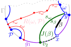
Figure 18: Case (e) of Observation 1, where $T(\beta)$ has no leaf on $\mathcal{P}$. Endpoint $x$ lies on a fine $\Gamma$-arc $g_{1}$ bounding $R(\omega,\mathcal{P})$, and $y\in\omega$.

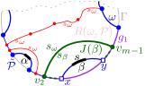
Figure 19: Case (d) of Observation 1, where $T(\beta)$ has no leaf on $\mathcal{P}$. Both $x,y$ lie on a fine $\Gamma$-arc $g_{1}$ bounding $R(\omega,\mathcal{P})$.

Lemma 9.

Given $\alpha$, $\gamma$, and $\mathcal{V}_{l}(\mathcal{P})$, the merge curve $J(\beta)$ can be computed in time $O(|J(\beta)|+d_{1}(\beta,\mathcal{P}_{\beta})+d_{2}(\beta,\mathcal{P}_{\beta})+r(\beta,\mathcal{P}_{\beta})+\tilde{d}(\beta,\mathcal{P}_{\beta}))$.

Proof.

We assume a ccw ordering of $\mathcal{P}$. We first determine the endpoints of $\beta$ in time $O(d_{1}(\beta,\mathcal{P}_{\beta})+d_{2}(\beta,\mathcal{P}_{\beta}))$ by scanning sequentially the arcs in $\mathcal{P}$ starting at $\alpha$ and moving ccw (towards $\gamma$) until the endpoints of $\beta$ are determined. Note that $\beta$ contains $\beta^{*}$ therefore we can easily identify the correct component of $J(s,s_{\beta})\cap D_{\mathcal{P}}$ during the scan, even if $J(s,s_{\beta})$ intersects $\mathcal{P}$ multiple times. This scan further determines which case of Observation 1 is relevant.

Let $T(\beta)$ denote the portion of $\mathcal{V}_{l}(\mathcal{P})$ that is enclosed by $J(\beta)$ and $\mathcal{P}\setminus\mathcal{P}_{\beta}$; this is deleted by the insertion of $\beta$. $T(\beta)$ is a plane forest, which by Theorem 2 is incident to the following faces of $\mathcal{V}_{l}(\mathcal{P})$: one face for each bisector edge of $J(\beta)$, and one face for each auxiliary arc $\alpha^{\prime}\in\mathcal{P}\setminus\mathcal{P}_{\beta}$. The latter number is counted in $d_{2}(\beta,\mathcal{P}_{\beta})$. We infer that $T(\beta)$ has complexity $O(|J(\beta)|+d_{2}(\beta,\mathcal{P}_{\beta}))$.

To compute $J(\beta)$ we trace $T(\beta)$ in time $O(|T(\beta)|)$, as for any ordinary Voronoi diagram, and this is possible due to Theorem 2 and Lemma 8. However, we first need to identify one leaf of $T(\beta)$.

Suppose first that $T(\beta)$ has a leaf on $\mathcal{P}$. Then, in all cases of Observation 1, except cases (d) and (e), a leaf of $T(\beta)$ is identified by the initial scan. In case (e), $\beta$ has at least one endpoint on a boundary arc $\rho$ of $\mathcal{P}$, see Fig. 16. We identify a leaf by scanning $\tilde{\mathcal{P}}$ starting at $\rho$ and moving towards the other endpoint of $\beta$. The scan takes only one step as the leaf will be incident to the first $\Gamma$-arc neighboring $\rho$ on $\tilde{\mathcal{P}}$. In case (d) both endpoints of $\beta$ are on $\Gamma$. We scan $\tilde{\mathcal{P}}$ from $\alpha$ to $\beta$ until we locate the first endpoint of $\beta$, $x$. A leaf of $T(\beta)$ must be incident to the fine $\Gamma$-arc that contains $x$. Since the encountered $\Gamma$-arcs remain in $\tilde{\mathcal{P}}_{\beta}$, the term $O(\tilde{d}(\beta,\mathcal{P}_{\beta}))$ is added to the overall time complexity.

Suppose now that $T(\beta)$ has no leaf on $\mathcal{P}$. Then $\beta$ is enclosed within a single Voronoi-like region $R(\omega,\mathcal{P})$. There are three cases Observation 1 (c), (d), and (e) to consider.

In case Observation 1(c), the insertion of $\beta$ splits arc $\omega$ in two parts, $\omega_{1}$ and $\omega_{2}$. To identify a leaf of $T(\beta)$ we scan $\partial R(\omega,\mathcal{P})$ sequentially until an intersection with $J(s_{\omega},s_{\beta})$ is found. We start scanning from both endpoints of $\omega$, tracing the shorter among $\partial R(\omega_{1},\mathcal{P}_{\beta})$ and $\partial R(\omega_{2},\mathcal{P}_{\beta})$. This adds the term $r(\beta,\mathcal{P}_{\beta})$ to the overall time complexity.

In cases Observation 1(d),(e), $J(\beta)\subseteq R(\omega,\mathcal{P})\cup\Gamma$, since otherwise $J(\beta)$ would intersect the region $R(\omega,\mathcal{P})$ twice, contradicting Theorem 2. Thus, $J(\beta)$ consists of a single bisector $J(s_{\omega},s_{\beta})$ and one ($m=3$) or two ($m=4$) $\Gamma$-arcs see Figs. 19 and 19. Thus, it is enough to identify $\omega$. In case (e), $\omega$ is identified during the initial scan. In case (d), $\beta$ has both endpoints on $\Gamma$. We scan $\tilde{\mathcal{P}}$ from $\alpha$ to $\beta$ until we locate the first endpoint of $\beta$, $x$. Then the $\Gamma$-arc that contains $x$ in $\tilde{\mathcal{P}}$ bounds the region $R(\omega,\mathcal{P})$. This scan adds the term $O(\tilde{d}(\beta,\mathcal{P}_{\beta}))$ to the time complexity. ∎

4.1 Proving Theorem 2

We first establish the following lemma.

Lemma 10.

$J(\beta)$ cannot intersect arc $\beta$, other than its endpoints.

Proof.

Suppose that an edge $e_{i}$ of $J(\beta)$, such that $e_{i}\subseteq J(s_{\alpha},s_{\beta})$ and $e_{i}\in R(\alpha,\mathcal{P})$, intersects arc $\beta$. Then $J(s,s_{\alpha})$ must also pass through the same intersection point within $R(\alpha,\mathcal{P})$. But an $s$-bisector $J(s,s_{\alpha})$ can never intersect $R(\alpha,\mathcal{P})$, by Lemma 5. ∎

We use the following observation throughout the proofs in this section.

Lemma 11.

For any $p\in S$, $D(s,p)\cap D_{\mathcal{P}}$ is connected. Thus, any components of the same $s$-bisector $J(s,\cdot)\cap D_{\mathcal{P}}$ must appear sequentially along $\mathcal{P}$.

Proof.

If we assume the contrary we obtain a forbidden $s$-inverse cycle defined by $J(s,\cdot)$ and $\mathcal{P}$. ∎

We now establish that $J(\beta)$ cannot pass through any region of auxiliary arcs in $\mathcal{P}\setminus\mathcal{P}_{\beta}$ that get deleted by the insertion of $\beta$.

Lemma 12.

Let $\alpha\in\mathcal{P}$ but $\alpha\not\in\mathcal{P}_{\beta}$. Then $R(\alpha,\mathcal{P})\subset D(s_{\beta},s_{\alpha})$.

Proof.

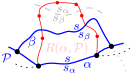
Figure 20: Illustrations for Lemma 12.

By Lemma 5, it holds that $R(\alpha,\mathcal{P})\subseteq D(s,s_{\alpha})$. Let $R_{s}=R(\alpha,\mathcal{P})\cap D(s,s_{\beta})$ and $R_{\beta}=R(\alpha,\mathcal{P})\cap D(s_{\beta},s)$. By transitivity of dominance regions we have $R_{\beta}\subseteq D(s_{\beta},s_{\alpha})$. By Lemma 11, $R_{s}$ is not incident to $\alpha$. Thus, if $J(s_{\beta},s_{\alpha})$ intersected $R_{s}$ then it would create a forbidden $s_{\alpha}$-cycle contradicting Lemma 6, see the dashed gray line in Fig. 20. This implies that also $R_{s}\subseteq D(s_{\beta},s_{\alpha})$. Thus, $R(\alpha,\mathcal{P})=R_{s}\cup R_{\beta}\subseteq D(s_{\beta},s_{\alpha})$. ∎

In the following we prove that $J(\beta)$ is an $s_{\beta}$-monotone path connecting the endpoints of $\beta$. To this aim we perform a bi-directional induction on the vertices of $J(\beta)$.

Let $J_{x}^{i}=(v_{1},v_{2},\ldots,v_{i}),1\leq i<m$, be the subpath of $J(\beta)$ starting at $v_{1}=x$ up to vertex $v_{i}$, including a small neighborhood of $e_{i}$ incident to $v_{i}$, see Fig. 16. Note that vertex $v_{i}$ uniquely determines $e_{i}$, however, its other endpoint is not yet specified. Similarly, let $J_{y}^{j}=(v_{m},v_{m-1},\ldots,v_{m-j+1}),1\leq j<m$, denote the subpath of $J(\beta)$, starting at $v_{m}$ up to vertex $v_{m-j+1}$, including a small neighborhood of edge $e_{m-j}$. For any bisector edge $e_{\ell}\in J(\beta)$, let $\alpha_{\ell}$ denote the boundary arc that induces $e_{\ell}$, i.e., $e_{\ell}\subseteq J(s_{\alpha_{\ell}},s_{\beta})\cap R(\alpha_{\ell},\mathcal{P})$.

Induction hypothesis: Suppose $J_{x}^{i}$ and $J_{y}^{j}$, $i,j\geq 1$, are disjoint $s_{\beta}$-monotone paths. Suppose further that each bisector edge of $J_{x}^{i}$ and of $J_{y}^{j}$ passes through a distinct region of $\mathcal{V}_{l}(\mathcal{P})$: $\alpha_{\ell}$ is distinct for $\ell$, $1\leq\ell\leq i$ and $m-j\leq\ell<m$, except possibly $\alpha_{i}=\alpha_{m-j}$ and $\alpha_{1}=\alpha_{m-1}$.

Induction step: Assuming that $i+j<m$, we prove that at least one of $J_{x}^{i}$ or $J_{y}^{j}$ can respectively grow to $J_{x}^{i+1}$ or $J_{y}^{j+1}$ at a valid vertex (Lemmas 13, 14), and it enters a new region of $\mathcal{V}_{l}(\mathcal{P})$ that has not been visited so far (Lemma 16). A valid vertex belongs in $\mathcal{A}(\mathcal{J}_{s_{\beta},S_{\mathcal{P}}}\cup\Gamma)$ or is an endpoint of $\beta$. A finish condition when $i+j=m$ is given in Lemma 15. The base case for $i=j=1$ is trivially true.

Suppose that $e_{i}\subseteq J(s_{\alpha_{i}},s_{\beta})$ and $v_{i}\in\partial R(\alpha_{i},\mathcal{P})$. To show that $v_{i+1}$ is a valid vertex it is enough to show that (1) $v_{i+1}$ can not be on $\alpha_{i}$, and (2) if $v_{i}$ is on a $\Gamma$-arc then $v_{i+1}$ can be determined on the same $\Gamma$-arc. However, we cannot easily derive these conclusions directly. Instead we show that if $v_{i+1}$ is not valid then $v_{m-j}$ will have to be valid.

In the following lemmas we assume that the induction hypothesis holds.

Lemma 13.

Suppose $e_{i}\subseteq J(s_{\alpha_{i}},s_{\beta})$ but $v_{i+1}\in\alpha_{i}$, that is, $e_{i}$ hits arc $\alpha_{i}\in\mathcal{P}$, and thus, $v_{i+1}$ is not a valid vertex. Then vertex $v_{m-j}$ must be a valid vertex in $\mathcal{A}(\mathcal{J}_{s_{\beta},S_{\mathcal{P}}})$, and $v_{m-j}$ can not be on $\mathcal{P}$.

Proof.

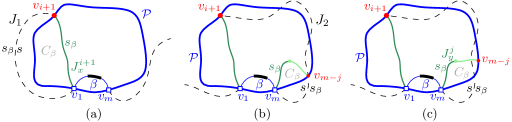
Figure 21: The assumption that edge $e_{i}=(v_{i},v_{i+1})$ of the merge curve $J_{x}^{i}$ hits a boundary arc of $\mathcal{P}$ as in Lemma 13.

Suppose vertex $v_{i+1}$ of $e_{i}$ lies on arc $\alpha_{i}$ as shown in Fig. 21(a). Vertex $v_{i+1}$ is the intersection point of related bisectors $J(s,s_{\alpha_{i}})$, $J(s_{\beta},s_{\alpha_{i}})$ and thus also of $J(s,s_{\beta})$. Thus, $v_{1},v_{m},v_{i+1}\in J(s,s_{\beta})$. By the induction hypothesis, no other vertex of $J_{x}^{i}$ nor $J_{y}^{j}$ can be on $J(s,s_{\beta})$. Vertices $v_{1},v_{i+1},v_{m}$ appear on $\mathcal{P}$ in clockwise order, because $J_{x}^{i+1}$ cannot intersect $\beta$. Arc $\beta$ partitions $J(s,s_{\beta})$ in two parts: $J_{1}$ incident to $v_{1}$ and $J_{2}$ incident to $v_{m}$. We claim that $v_{i+1}$ must lie on $J_{2}$, as otherwise, $J_{x}^{i+1}$ and $J_{1}$ would form a forbidden $s_{\beta}$-inverse cycle, see the dashed black and the green solid curve in Fig. 21(a), contradicting Lemma 2. This cycle must be $s_{\beta}$-inverse because $J_{x}^{i+1}\subseteq\overline{D_{\mathcal{P}}}$, and all components of $J(s,\cdot)\cap D_{\mathcal{P}}$ must appear sequentially along $\mathcal{P}$ by Lemma 11.

Thus, $v_{i+1}$ lies on $J_{2}$. Further, by Lemma 11, the components of $J_{2}\cap D_{\mathcal{P}}$ appear on $\mathcal{P}$ clockwise after $v_{i+1}$ and before $v_{m}$, as shown in Fig. 21(b), which illustrates $J(s,s_{\beta})$ as a black dashed curve.

Now consider $J_{y}^{j}$. We show that $v_{m-j}$ cannot be on $\mathcal{P}$. First observe that $v_{m-j}$ can not lie on $\mathcal{P}$, clockwise after $v_{m}$ and before $v_{1}$, since $J_{y}^{j+1}$ cannot cross $\beta$. Now we prove that $v_{m-j}$ cannot lie on $\mathcal{P}$ clockwise after $v_{1}$ and before $v_{i+1}$. To see that, note that edge $e_{m-j}$ cannot cross any non-$\Gamma$ edge of $J_{x}^{i+1}$, because by the induction hypothesis, $\alpha_{m-j}$ is distinct from all $\alpha_{\ell},\ell\leq i$. In addition, by the definition of a $\Gamma$-arc, $v_{m-j}$ cannot lie on any $\Gamma$-arc of $J_{x}^{i}$. Finally, we show that $v_{m-j}$ cannot lie on $\mathcal{P}$ clockwise after $v_{i+1}$ and before $v_{m}$. If $v_{m-j}$ lay on the boundary arc $\alpha_{m-j}$ then we would have $v_{m-j}\in J(s,s_{\beta})$. This would define an $s_{\beta}$-inverse cycle $C_{\beta}$, formed by $J_{y}^{j+1}$ and $J(s_{\beta},s)$, see Fig. 21(b), similarly to the first paragraph of this proof. If $v_{m-j}$ lay on a $\Gamma$-arc then there would also be a forbidden $s_{\beta}$-inverse cycle formed by $J_{y}^{j+1}$ and $J(s,s_{\beta})$ because in order to reach $\Gamma$, edge $e_{i}$ must cross $J(s,s_{\beta})$. See the dashed black and the green curve in Fig. 21(c). Thus $v_{m-j}\not\in\mathcal{P}$.

Since $v_{m-j}\in\partial R(\alpha_{i+1})$ but $v_{m-j}\not\in\mathcal{P}$, it must be a vertex of $\mathcal{A}(\mathcal{J}_{s_{\beta},S_{\mathcal{P}}})$. ∎

The proof for the following lemma is similar.

Lemma 14.

Suppose vertex $v_{i}$ is on a $\Gamma$-arc $g\in\mathcal{P}$ but $v_{i+1}$ cannot be determined because no bisector $J(s_{\beta},s_{\gamma})$ intersects $\overline{R(\gamma,\mathcal{P})}\cap g$, clockwise from $v_{i}$. Then vertex $v_{m-j}$ must be a valid vertex in $\mathcal{A}(\mathcal{J}_{s_{\beta},S_{\mathcal{P}}})$ and $v_{m-j}$ can not be on $\mathcal{P}$.

Proof.

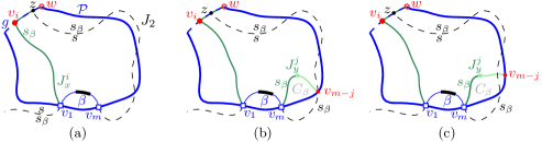
Figure 22: The assumption that $v_{i}\in\Gamma$ and $v_{i+1}$ of the merge curve $J_{x}^{i}$ cannot be determined as in Lemma 14.

We truncate the $\Gamma$-arc $g$ to its portion clockwise from $v_{i}$; let $w$ be the endpoint of $g$ clockwise from $v_{i}$, see Fig. 22(a). If no $J(s_{\beta},s_{\gamma})\cap R(\gamma,\mathcal{P})$ intersects $g$, as we assume in this lemma, then $R(\gamma,\mathcal{P})\cap g\subseteq D(s_{\beta},s_{\gamma})$, for any region $R(\gamma,\mathcal{P})$ incident to $g$. Thus, $w\in D(s_{\beta},s)$. However, $v_{i}\in D(s,s_{\beta})$, since, by Lemma 5, $R(\alpha_{i-1})\subseteq D(s,s_{\alpha_{i-1}})$ and $v_{i}$ is incident to $J(s_{\beta},s_{\alpha_{i-1}})\cap R(\alpha_{i-1})$. Thus, $J(s,s_{\beta})$ must intersect $g$ at some point $z$ clockwise from $v_{i}$. Arc $\beta$ partitions $J(s,s_{\beta})$ in two parts: $J_{1}$ incident to $v_{1}$ and $J_{2}$ incident to $v_{m}$. Lemma 11 implies that all components of $J_{2}\cap D_{\mathcal{P}}$ appear on $\mathcal{P}$ clockwise after $v_{i}$ and before $v_{m}$, as shown by the black dashed curve in Fig. 22(a); also $z$ lies on $J_{2}$.

Now we can show that vertex $v_{m-j}$ of $J_{y}^{j}$ cannot be on $\mathcal{P}$ analogously to the proof of Lemma 13. The only difference is that we must additionally show that $v_{m-j}$ cannot lie on $\mathcal{P}$ clockwise after $v_{i}$ and before $w$. But this holds already by the assumption in the lemma statement. Refer to Figures 22(b) and (c).

We conclude that $v_{m-j}$ cannot lie on $\mathcal{P}$ and it is a valid vertex of $\mathcal{A}(\mathcal{J}_{s_{\beta},S_{\mathcal{P}}})$. ∎

Lemma 15 in the sequel provides a finish condition for the induction, when $J_{x}^{i}$ and $J_{y}^{j}$ are incident to a common region or to a common $\Gamma$-arc. When it is met, the merge curve $J(\beta)$ is a concatenation of $J_{x}^{i}$ and $J_{y}^{j}$.

Lemma 15.

Suppose $i+j>2$ and either (1) or (2) holds: (1) $v_{i}$ and $v_{m-j+1}$ are incident to a common region $R(\alpha_{i},\mathcal{P})$ and $e_{i},e_{m-j}\subseteq J(s_{\beta},s_{\alpha_{i}})$, i.e., $\alpha_{i}=\alpha_{m-j}$; or (2) $v_{i}$ and $v_{m-j+1}$ are on a common $\Gamma$-arc $g$ of $\mathcal{P}$ and $e_{i},e_{m-j}\subseteq\Gamma$. Then $v_{i+1}=v_{m-j+1}$, $v_{m-j}=v_{i}$, and $m=i+j$.

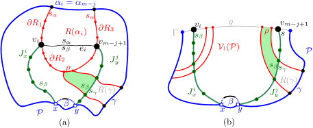
Figure 23: Illustrations for Lemma 15. (a) corresponds to condition (1) and (b) to condition (2). Here, the label $R(\gamma)$ abbreviates $R(\gamma,\mathcal{P})$.

Proof.

Let $\alpha=\alpha_{i}$. Suppose (1) holds, then $e_{i},e_{m-j}\subseteq J(s_{\beta},s_{\alpha})$, see Fig. 23(a). The boundary $\partial R(\alpha_{i},\mathcal{P})$ is partitioned in four parts, using a counterclockwise traversal starting at $\alpha_{i}$: $\partial R_{1}$, from the endpoint of arc $\alpha_{i}$ to $v_{i}$; $\partial R_{2}$, from $v_{i}$ to $v_{m-j+1}$; $\partial R_{3}$, from $v_{m-j+1}$ to the next endpoint of $\alpha_{i}$; and arc $\alpha_{i}$. We show that $e_{i}$ and $e_{m-j}$ cannot hit any of these parts; thus, $e_{i}=e_{m-j}$.

1. Edge $e_{i}$ cannot hit $\partial R_{1}$ and edge $e_{m-j}$ cannot hit $\partial R_{3}$ by the cut property, Lemma 7.

2. We prove that edge $e_{i}$ cannot hit $\partial R_{2}$. Analogously for edge $e_{m-j}$. Let $\rho$ be any edge on $\partial R_{2}$. (If $v_{i}\in\rho$ or $v_{m-j+1}\in\rho$, assume that $\rho$ is truncated with endpoint $v_{i}$ or $v_{m-j+1}$ respectively).

   1. Suppose that $\rho$ is a bisector edge, $\rho\subseteq J(s_{\alpha},s_{\gamma})$, see Fig. 23(a). Then at least one of $J_{y}^{j}$, $J_{x}^{i}$, or $\beta$ must pass through $R(\gamma,\mathcal{P})$. Suppose that $J_{y}^{j}$ does, as shown in Fig. 23(a). Then by the cut property (Lemma 7) $\rho\subseteq D(s_{\beta},s_{\gamma})$. By transitivity (Lemma 3) it also holds that $\rho\subseteq D(s_{\beta},s_{\alpha})$. Thus, $e_{i}$ cannot hit $\rho$. Symmetrically for $J_{x}^{i}$. If only $\beta$ passes through $R(\gamma,\mathcal{P})$, then we can use Lemma 12 to derive that $\rho\subseteq D(s_{\beta},s_{\gamma})$; the rest follows.

   2. Suppose that $\rho\subseteq\Gamma$. Then either $\rho$ itself is part of an edge of $J_{y}^{j}$ or of $J_{x}^{i}$, or $\beta$ passes through $R(\alpha,\mathcal{P})$ and $\rho$ is at opposite side of it than $\alpha$. In the former case, $\rho\subseteq D(s_{\beta},s_{\alpha})$ by the definition of a $\Gamma$-edge in the merge curve. In the latter case, the same is derived by Lemma 5 and transitivity (Lemma 3). Thus, $e_{i}$ cannot hit $\rho$.

3. Edge $e_{i}$ (resp. $e_{m-j}$) cannot hit $\partial R_{3}$ because if it did, $e_{i}$ and $e_{m-j}$ would not appear sequentially on $R(\alpha_{i},\mathcal{P})$ contradicting Lemma 7.

4. It remains to show that $e_{i}$ and $e_{m-j}$ cannot both hit $\alpha_{i}$. But this is already shown in Lemma 13.

Now suppose (2) holds, see Fig. 23(b). Let $R(\gamma,\mathcal{P})$ be a region in $\mathcal{V}_{l}(\mathcal{P})$ incident to the $\Gamma$-arc $g$ and let $\rho=R(\gamma,\mathcal{P})\cap g$ be the $\Gamma$-arc bounding $R(\gamma,\mathcal{P})$, which lies between $v_{i}$ and $v_{m-j+1}$. At least one of $J_{y}^{j}$ or $J_{x}^{i}$ or $\beta$ must pass through $R(\gamma,\mathcal{P})$. By the exact same arguments as before, $\rho\subseteq D(s_{\beta},s_{\gamma})$. We infer that there is no bisector $J(s_{\beta},s_{\gamma})$ in $R(\gamma,\mathcal{P})$, for any region $R(\gamma,\mathcal{P})$ incident to $g$ between $v_{i}$ and $v_{m-j+1}$. Thus, $e_{i+1}=e_{m-j+1}\subseteq g$.

Thus, in both (1) and (2) $v_{i+1}=v_{m-j+1}$, $v_{m-j}=v_{i}$, and $m=i+j$. $J(\beta)$ is the concatenation of $J_{x}^{i}$ and $J_{y}^{j}$ with $e_{i+1}=e_{m-j+1}$. ∎

Lemma 16.

Suppose vertex $v_{i+1}$ is valid and $e_{i+1}\subseteq J(s_{\beta},s_{a_{i+1}})$. Then $R(\alpha_{i+1})$ has not been visited by $J_{x}^{i}$ nor $J_{y}^{j}$, i.e., $\alpha_{i+1}\neq\alpha_{\ell}$ for $\ell\leq i$ and for $m-j<\ell$.

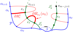
Figure 24: Illustration for Lemma 16.

Proof.

Let $e_{k},k\leq i$, be a bisector edge of $J_{x}^{i}$. Denote by $\partial R_{k}^{1}$ the portion of $\partial R(\alpha_{k})$ from $\alpha_{k}$ to $v_{k}$ in a counterclockwise traversal, see the bold red part $\partial R_{i}^{1}$ in Fig. 24. Analogously for a bisector edge $e_{m-j}$ of $J_{y}^{j}$, where $\partial R_{m-j}^{1}$ is defined in a clockwise traversal of $\partial R(\alpha_{m-j})$. Recall that $\partial R_{e_{k}}(\alpha_{k})$, denotes the portion of $\partial R(\alpha_{k})$ cut out by edge $e_{k}$, at opposite side from $\alpha_{k}$.

The cut property of Lemma 7 implies that $v_{i+1}$ cannot be on $\partial R_{e_{\ell}}(\alpha_{\ell})$ for any $\ell$, $\ell<i$ and $m-j<\ell$ and that $v_{i+1}$ cannot be on $\partial R_{i}^{1}$. This implies that $v_{i+1}$ cannot be on $\partial R_{\ell}^{1}$ for any $\ell<i$, because we have a plane graph in $D_{\mathcal{P}}$ and by its layout $\partial R_{\ell}^{1}$ is not reachable from $e_{i}$ without first hitting $\partial R_{e_{\ell}}(\alpha_{\ell})$ or $\partial R_{i}^{1}$. See Fig. 24. Thus, $v_{i+1}$ can not be on $\partial R(\alpha_{\ell})$, $\ell<i$. By Lemma 15 $v_{i+1}$ cannot be on $\partial R_{m-j}^{1}$. This implies, again by the layout, that $v_{i+1}$ cannot be on $\partial R_{\ell}^{1}$ for all $\ell>m-j$. Thus, $v_{i+1}$ can not be on $\partial R(\alpha_{\ell})$, for any $\ell>m-j$. This implies that $\alpha_{i+1}\neq\alpha_{\ell}$, for any $\ell$, $\ell\leq i$ or $\ell>m-j$. ∎

By Lemma 16, $J_{x}^{i+1}$ and $J_{y}^{j+1}$ always enter a new region of $\mathcal{V}_{l}(\mathcal{P})$ that has not been visited in any previous step. Hence, conditions (1) or (2) of Lemma 15 must be fulfilled at some point of the induction, completing the proof of Theorem 2.

Completing the bi-directional induction establishes also the remaining properties for $J(\beta)$. First, $J(\beta)$ can never enter the same region twice (by Lemma 16), except the region of $\alpha_{1}$, if $\alpha_{1}=\alpha_{m}$. This is Observation 1(c), where arc $\beta$ splits a single arc $\alpha\in\mathcal{P}$. In this case $J(\beta)$ enters $R(\alpha,\mathcal{P})$ exactly twice and both $e_{1},e_{m-1}\subseteq J(s_{\alpha},s_{\beta})$. This is because $J(\beta)$ must intersect $\partial R(\alpha,\mathcal{P})$, i.e., $J(\beta)\not\subseteq R(\alpha,\mathcal{P})$, as otherwise $J(\beta)=J(s_{\alpha},s_{\beta})$ (see Fig. 16) contradicting the labeling of the cut property in Lemma 7.

Completing the induction for Theorem 2 establishes also that $J(\beta)$ is unique and that the conditions of Lemmas 13 and 14 can never be met. Thus, no vertex of $J(\beta)$, except its endpoints, can be on a boundary arc of $\mathcal{P}$.

5 $\mathcal{V}_{l}(\mathcal{P})$ is unique

In this section we prove Theorem 1 and establish that for a boundary curve $\mathcal{P}$ on $\mathscr{S}^{\prime}\subseteq\mathscr{S}$, the Voronoi-like diagram $\mathcal{V}_{l}(\mathcal{P})$ is unique.

We first show an essential property of Voronoi-like regions, which completes the cut property of Lemma 7.

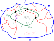
Figure 25: A component $e$ of $J(s_{\alpha},\cdot)$ in $R(\alpha,\mathcal{P})$ as in Lemma 17.

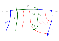
Figure 26: A component $e$ of $J(s_{\alpha},\cdot)$ in $R(\alpha,\mathcal{P})$ with its endpoint $v$ on a $\Gamma$-arc $g$ as in Lemma 17.

Lemma 17.

Let $\beta^{*}\in\mathscr{S}^{\prime}$ and $\beta^{*}\subseteq J(s,s_{\beta})$. Suppose that a component $e$ of $J(s_{\alpha},s_{\beta})$ intersects $R(\alpha,\mathcal{P})$ in $\mathcal{V}_{l}(\mathcal{P})$. Then $J(s,s_{\beta})$ must also intersect the domain $D_{\mathcal{P}}$. Further, there exists a component $\beta$ of $J(s,s_{\beta})\cap D_{\mathcal{P}}$ such that the merge curve $J(\beta)$ in $\mathcal{V}_{l}(\mathcal{P})$ contains $e$ (i.e., $e\subset\partial R(\beta,\mathcal{P}\oplus\beta)$).

We say that arc $\beta$ is missing from $\mathcal{P}$.

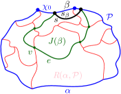
Figure 27: Arc $\beta\subseteq J(s,s_{\beta})$ in $D_{\mathcal{P}}$; The merge curve $J(\beta)$ contains $e$.

Proof.

Suppose there is a non-empty component $e$ of $J(s_{\alpha},s_{\beta})\cap R(\alpha,\mathcal{P})$, however, $J(s,s_{\beta})\cap D_{\mathcal{P}}=\emptyset$, thus, $D_{\mathcal{P}}\subseteq D(s,s_{\beta})$. By the transitivity of dominance regions (Lemma 3), it follows that for any arc $\chi\in\mathcal{P}$, $\chi\subseteq D(s_{\chi},s_{\beta})$. Let $R_{e}(\alpha)$ denote the portion of $R(\alpha,\mathcal{P})$ cut out by $e$ (at opposite side from $\alpha$) as defined in Lemma 7; then $\partial R_{e}(\alpha)\subseteq D(s_{\beta},s_{\alpha})$.

Consider an endpoint $v$ of $e$. There are two cases:

1. If $v$ is on an edge $\rho$ incident to regions $R(\alpha,\mathcal{P})$ and $R(\gamma,\mathcal{P})$, then $J(s_{\beta},s_{\gamma})$ intersects $R(\gamma,\mathcal{P})$ by an edge $e_{\rho}$, incident to $v$, leaving $\rho$ and $\gamma$ at opposite sides, because $\gamma\subseteq D(s_{\gamma},s_{\beta})$, see Fig. 26.

2. If $v$ is on a $\Gamma$-arc $g$, let $R(\gamma,\mathcal{P})$ be the first region after $v$ (towards $D(s_{\beta},s_{\alpha})$) with $J(s_{\beta},s_{\gamma})$ intersecting $g\cap\overline{R(\gamma,\mathcal{P})}$ at point $u$, see Fig. 26. There exists such $R(\gamma,\mathcal{P})$ because for all boundary arcs $\chi\in\mathcal{P}$, $\chi\subseteq D(s_{\chi},s_{\beta})$, and this includes the boundary arc that is incident to $g$. Let $e_{g}$ be the component of $J(s_{\beta},s_{\gamma})\cap R(\gamma,\mathcal{P})$ incident to $u$.

Thus, given $e$ and $v$, we derive an edge $e^{\prime}$, either $e^{\prime}=e_{\rho}$ or $e^{\prime}=e_{g}$, with the same properties as $e$, in a different region of $\mathcal{V}_{l}(\mathcal{P})$. This process repeats and there is no way to break it because for any arc $\chi\in\mathcal{P}$, $\chi\subseteq D(s_{\chi},s_{\beta})$. Thus, we create a closed curve on $\mathcal{V}_{l}(\mathcal{P})$ consisting of consecutive pieces of $J(s_{\beta},.)$, possibly interleaved with $\Gamma$-arcs, which has the label $s_{\beta}$ in its interior. No two edges of this curve can intersect because otherwise the bisector corresponding to such intersecting edges would not be a Jordan curve. Furthermore, no vertex of this curve can repeat under our general position assumption as no three $s_{\beta}$-related bisectors can intersect at the same point. Thus, the closed curve must be an $s_{\beta}$-cycle $C$ that is contained in $D_{\mathcal{P}}$, see Fig. 26, which contradicts Lemma 6. Thus, our assumption that $J(s,s_{\beta})\cap D_{\mathcal{P}}=\emptyset$ was false, and thus, $J(s,s_{\beta})$ must intersect $\mathcal{P}$. The above process must encounter such an intersection as otherwise the forbidden $s_{\beta}$-cycle $C$ would exist. Let $J_{e}(\beta)$ denote the sequence of encountered edges $e_{\rho}$, starting with the initial edge $e$ and ending on the first intersection of an arc $\chi_{0}$ in $\mathcal{P}$ with $J(s,s_{\beta})$. Let $\beta$ be the component of $J(s,s_{\beta})\cap D_{\mathcal{P}}$ incident to $\chi_{0}$, see Fig. 27.

By its definition, the path $J_{e}(\beta)$ fulfills the definition of the merge curve $J(\beta)$ (Definition 5). Since by Theorem 2 the merge curve $J(\beta)$ on $\mathcal{V}_{l}(\mathcal{P})$ is unique, it follows that $J(\beta)$ contains $J_{e}(\beta)$, and thus, it also contains edge $e$. ∎

We can now prove Theorem 1 from Section 3.

$\blacktriangleright$ Theorem 1. Given a boundary curve $\mathcal{P}$ for $\mathscr{S}^{\prime}\subseteq\mathscr{S}$, $\mathcal{V}_{l}(\mathcal{P})$ is unique.

Proof.

Let $\mathcal{P}$ be a boundary curve for $\mathscr{S}^{\prime}\subseteq\mathscr{S}$ such that $\mathcal{P}$ admits a Voronoi-like diagram $\mathcal{V}_{l}(\mathcal{P})$. Suppose there exist two different Voronoi-like diagrams of $\mathcal{P}$, $\mathcal{V}_{l}^{(1)}\neq\mathcal{V}_{l}^{(2)}$. Then there must be an edge $e^{(1)}$ of $\mathcal{V}_{l}^{(1)}$ bounding regions $R^{(1)}(\alpha,\mathcal{P})$ and $R^{(1)}(\beta,\mathcal{P})$ of $\mathcal{V}_{l}^{(1)}$, where $\alpha,\beta\in\mathcal{P}$, such that $e^{(1)}$ intersects region $R^{(2)}(\alpha,\mathcal{P})$ of $\mathcal{V}_{l}^{(2)}$, since $\alpha$ is common to both $R^{(1)}(\alpha,\mathcal{P})$ and $R^{(2)}(\alpha,\mathcal{P})$.

Let edge $e\subseteq J(s_{\beta},s_{\alpha})$ be the component of $R^{(2)}(\alpha,\mathcal{P})\cap J(s_{\beta},s_{\alpha})$ overlapping with $e^{(1)}$, see Fig. 28. From Lemma 17 it follows that there is a non-empty component $\beta_{0}$ of $J(s,s_{\beta})\cap D_{\mathcal{P}}$ such that $J(\beta_{0})$ in $\mathcal{V}_{l}^{(2)}$ contains edge $e$. Since $J(\beta_{0})$ and $\partial R^{(1)}(\beta,\mathcal{P})$ have an overlapping portion $\left(e\cap e^{(1)}\right)$ and they bound the regions of two different arcs $\beta_{0}\neq\beta$ of site $s_{\beta}$, they form an $s_{\beta}$-cycle $C$ as shown in Fig. 28. But $C$ is contained in $D_{\mathcal{P}}$, deriving a contradiction to Lemma 6. ∎

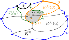
Figure 28: Illustrations for the proof of Theorem 1.

6 A randomized incremental algorithm

Consider a random permutation $o=(\alpha_{1},\dots,\alpha_{h})$ of the set of core arcs $\mathscr{S}$, where $|\mathscr{S}|=h$. For $1\leq i\leq h$, define set $\mathscr{S}_{i}=\{\alpha_{1},\dots,\alpha_{i}\}\subseteq\mathscr{S}$ to be the subset of the first $i$ arcs in $o$, and permutation $o_{i}=(\alpha_{1},\dots,\alpha_{i})$. Let $\mathcal{P}_{i}$ denote the boundary curve derived by the arc insertion operation $\oplus$ by considering arcs in the order $o_{i}$. Let $D_{i}$ denote the corresponding domain enclosed by $\mathcal{P}_{i}$.

Our randomized algorithm is inspired by the randomized, two-phase, approach of Chew [7] for the Voronoi diagram of points in convex position; however, the sites are core arcs in $\mathscr{S}$, forming boundary curves, and the algorithm constructs Voronoi-like diagrams within a series of shrinking domains $D_{i}\supseteq D_{i+1}$. The domain $D_{1}$ is $D(s,s_{\alpha_{1}})\cap D_{\Gamma}$; and $D_{h}$ coincides with the Voronoi region $\mbox{VR}(s,S)\cap D_{\Gamma}$. The boundary curves are obtained by the insertion operation $\oplus$, one at each step, starting with $\mathcal{P}_{1}=J(s,s_{\alpha_{1}})\cap D_{\Gamma}$, and ending with $\mathcal{P}_{h}=\partial\mbox{VR}(s,S)\cap D_{\Gamma}$. The algorithm works in two phases.

In phase 1, the arcs in $\mathscr{S}$ get deleted one by one, in reverse order of $o$, while recording the neighbors of each arc at the time of its deletion. Let $\mathcal{P}_{1}=J(s,s_{\alpha_{1}})\cap D_{\Gamma}$, $R(\alpha_{1},\mathcal{P}_{1})=D(s,s_{\alpha_{1}})\cap D_{\Gamma}$, and $\mathcal{V}_{l}(\mathcal{P}_{1})=\emptyset$.

In phase 2, we start with $\mathcal{V}_{l}(\mathcal{P}_{1})$ and incrementally compute $\mathcal{V}_{l}(\mathcal{P}_{i})$, $i=2,\dots,h$, by inserting arc $\alpha_{i}$, where $\mathcal{P}_{i}=\mathcal{P}_{i-1}\oplus\alpha_{i}$, and $\mathcal{V}_{l}(\mathcal{P}_{i})=\mathcal{V}_{l}(\mathcal{P}_{i-1})\oplus\alpha_{i}$. When inserting an arc $\alpha_{i}$, we use the information of its recorded neighbors from phase 1 to determine its insertion point. At the end we obtain $\mathcal{V}_{l}(\mathcal{P}_{h})$, where $\mathcal{P}_{h}$ is a boundary curve of $\mathscr{S}$. The set $\mathscr{S}$ has one unique boundary curve that coincides with its $s$-envelope. Thus, $\mathcal{P}_{h}$ can contain no auxiliary arcs and $\mathcal{P}_{h}=\text{env}(\mathscr{S})=\partial\mbox{VR}(s,S)\cap D_{\Gamma}$.

We have already established that the Voronoi-like diagram of an $s$-envelope $\mathcal{E}$ is the real Voronoi diagram $\mathcal{V}(\mathcal{E})$ (Corollary 1). We have also established the correctness of the insertion operation $\oplus$. Thus, the algorithm correctly computes $\mathcal{V}_{l}(\mathcal{P}_{h})$, where $\mathcal{V}_{l}(\mathcal{P}_{h})=\mathcal{V}(\mathscr{S})=\mathcal{V}(S\setminus\{s\})\cap\mbox{VR}(s,S)\cap D_{\Gamma}$.

Next we analyze the time complexity of this algorithm and prove that the time complexity of step-$i$ is expected $O(1)$; thus, the overall time complexity is expected $O(h)$.

Lemma 18.

$\mathcal{P}_{i}$ contains at most $i-1$ auxiliary arcs; thus, $|\mathcal{V}_{l}(\mathcal{P}_{i})|=O(i)$.

Proof.

By definition, $|\mathcal{P}_{1}|=1$. At each step of phase 2, exactly one original arc is inserted, and at most one additional auxiliary arc is created by a split in case (c) of Observation 1, except from $i=1$ and $i=h$. Thus, the total number of auxiliary arcs is at most $i-1$ and the number of original arcs is at most $i$. Since an original arc may be merged with its neighbor in case (f) of Observation 1, the number of original arcs in $\mathcal{P}_{i}$ may indeed be less than $i$. Since the complexity of $\mathcal{V}_{l}(\mathcal{P}_{i})$ is $O(|\mathcal{P}_{i}|)$, the claim follows. ∎

6.1 Time analysis of the randomized incremental algorithm

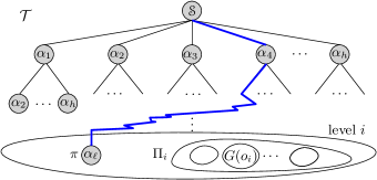
Figure 29: There are $h!/(h-i)!$ nodes at level-$i$ of the decision tree $\mathcal{T}$, each corresponding to a unique permutation of $i$ core arcs. Level $i$ is partitioned into groups of size $i$.

Consider the decision tree $\mathcal{T}$ of all possible random choices that can be made by our incremental algorithm on the input set of core arcs $\mathscr{S}$, $h=|\mathscr{S}|$, see Fig. 29. $\mathcal{T}$ has $h!$ leaves each corresponding to one permutation of the arcs in $\mathscr{S}$. At level-$i$, there are $h!/(h-i)!$ nodes, and each node corresponds to a unique permutation of $i$ core arcs. A set of $i$ core arcs $\mathscr{S}_{i}$ is associated with $i!$ different nodes at level-$i$, which are called the block of $\mathscr{S}_{i}$. We have ${h\choose i}$ distinct such blocks at level-$i$. Although all nodes within one block are associated with the same set of core arcs, their corresponding boundary curves may vary considerably depending on their permutation order. Because the boundary curves are order-dependent we cannot easily apply backwards analysis as in the original randomized incremental construction of Chew [7]. Instead, we establish the expected complexity of step-$i$ by analyzing each block of nodes at level-$i$ of $\mathcal{T}$ .

We use the following strategy. We partition each block at level-$i$ of $\mathcal{T}$ into $(i-1)!$ disjoint groups of $i$ nodes each. For each group we show that the step $i$ of the algorithm requires total time $O(i)$, for all the $i$ permutations within the group. Thus, on average, the algorithm spends $O(1)$ time on each node of $\mathcal{T}$. Since all permutations are equally likely, we obtain the expected linear ($O(h)$) time complexity of our algorithm.

Let $o_{i}=(\alpha_{1},\alpha_{2},\dots,\alpha_{i})$ be an arbitrary permutation of $\mathscr{S}_{i}$. From $o_{i}$ we define a group $G=G(o_{i})$ of $i$ permutations: for each $1\leq j<i$, remove ${\alpha_{j}}$ from its position in $o_{i}$ and append it to the end of $o_{i}$.

$$o_{i} =(\alpha_{1},\alpha_{2},\dots,\alpha_{j-1},\boxed{\alpha_{j}},{\alpha_{j+1}}\dots,\alpha_{i-1},\alpha_{i})$$ (1)

$$o_{j} =(\alpha_{1},\alpha_{2},\dots,\alpha_{j-1},\qquad\;{\alpha_{j+1}},\dots,\alpha_{i-1},\alpha_{i},\boxed{{\alpha_{j}}}),$$ (2)

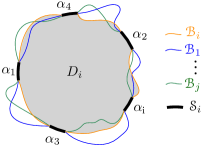
Figure 30: Schematic differences between the boundary curves $\mathcal{B}_{1},\dots,\mathcal{B}_{i}$. The domain $D_{i}$ is shown shaded.

Figure 31: Illustration for Definition 7, $o_{1}=(\beta,\alpha,\gamma)$: The core arc $\alpha\in\mathscr{S}_{i}$ is the source of $\alpha^{\prime}\in\text{in}_{1}$. The expanded arc $\tilde{\alpha}\supseteq\alpha^{\prime}$ was created when inserting $\alpha$ during the construction of $\mathcal{B}_{1}$. $\mathcal{B}_{i}$ for $o_{i}=(\gamma,\beta,\alpha)$ is shown in Fig. 32(a).

Let $\mathcal{B}_{j}$, $1\leq j\leq i$, denote the boundary curves derived by arc insertion following the order $o_{j}$, see Fig. 31. $\mathcal{B}_{i}$ is the base boundary curve derived from $o_{i}$, and its domain is denoted $D_{i}$. In the following we establish the relation between these boundary curves so that we can prove our objective regarding the time complexity of the $i$th step of the algorithm on all of them (Lemma 23). We first introduce some terminology.

Definition 7.

Let $\alpha^{\prime}$ be an auxiliary arc in $\mathcal{B}_{j}$ and let $\alpha\in\mathscr{S}_{i}$ be a core arc of the same site. We say that $\alpha^{\prime}$ is an auxiliary arc of the core arc $\alpha$ if there had been an expanded arc $\tilde{\alpha}\supseteq\alpha\cup\alpha^{\prime}$, which was created for the first time during the construction of $\mathcal{B}_{j}$ when inserting $\alpha$ (see Fig. 31). The core arc $\alpha\in\mathscr{S}_{i}$ is called the source of $\alpha^{\prime}$ and is denoted as $\text{source}_{j}(\alpha^{\prime})$.

If $\alpha^{\prime}$ appears counterclockwise (resp. clockwise) from its source $\alpha$ along their common $s$-bisector then $\alpha^{\prime}$ is called a ccw (resp. cw) auxiliary arc.

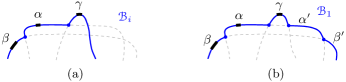
Figure 32: (a) Boundary curve $\mathcal{B}_{i}$, where $o_{i}=(\gamma,\beta,\alpha)$. (b) Boundary curve $\mathcal{B}_{1}$, where $o_{1}=(\beta,\alpha,\gamma)$, containing arcs $\alpha^{\prime},\beta^{\prime}\in\text{in}_{1}$, because ${\gamma}$ was inserted last.

The boundary curves $\mathcal{B}_{j}$, $j<i$, may get in and out of the domain $D_{i}$, see Fig. 31. To identify their differences from $\mathcal{B}_{i}$, let $\text{in}_{j}=\mathcal{B}_{j}\cap D_{i}$, and $\text{out}_{j}=\mathcal{B}_{j}\setminus\overline{D_{i}}$, denote the portion of $\mathcal{B}_{j}$ inside, and outside of $D_{i}$, respectively. We partition the auxiliary arcs in $\text{in}_{j}$ into $\text{in}_{j}^{+}$ and $\text{in}_{j}^{-}$, where $\text{in}_{j}^{+}$ (resp. $\text{in}_{j}^{-}$) includes the ccw (resp. cw) auxiliary arcs of $\text{in}_{j}$, see Fig. 32. In the following we only consider $\text{in}_{j}^{+}$ as $\text{in}_{j}^{-}$ is symmetric.

Observation 2.

The boundary curve $\mathcal{B}_{j}$, $j\neq i$, contains no auxiliary arcs of the core arc $\alpha_{j}$ (since $\alpha_{j}$ appears last in $o_{j}$), and these are the only auxiliary arcs of $\mathcal{B}_{i}$ that are missing from $\mathcal{B}_{j}$ (since the insertion order of all other core arcs is identical). Thus, any auxiliary arc $\alpha^{\prime}\in\text{out}_{j}$ must lie below an auxiliary arc of $\alpha_{j}$ in $\mathcal{B}_{i}$, see Fig. 33. Further, no region of an arc in $\text{out}_{j}$ can be adjacent to $R(\alpha_{j},\mathcal{B}_{j})$.

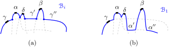
Figure 33: (a) Boundary curve $\mathcal{B}_{i}$, where $o_{i}=(\gamma,\alpha,\beta,\delta)$. (b) Boundary curve $\mathcal{B}_{1}$ containing arcs $\alpha^{\prime},\alpha^{\prime\prime}$ in $\text{out}_{1}$, where $o_{1}=(\alpha,\beta,\delta,\gamma)$.

Observation 3.

Let $\alpha^{\prime}\in\text{in}_{j}$ and let $\alpha_{k}=\text{source}_{j}(\alpha^{\prime})$. Then $k>j$, i.e., $\alpha_{k}$ follows $\alpha_{j}$ in $o_{i}$. Further, if $\alpha^{\prime}\in\text{in}_{j}^{+}$ then $(\alpha_{k},\alpha_{j},\alpha^{\prime})$ appear ccw in $\mathcal{B}_{j}$.

Observation 4.

Fig. 34 indicates the structure of $\text{in}_{j}^{+}$. Let $\alpha^{\prime},\beta^{\prime}\in\text{in}_{j}^{+}$ such that $\alpha_{k}=\text{source}_{j}(\alpha^{\prime})$, $\alpha_{\ell}=\text{source}_{j}(\beta^{\prime})$, and $k<\ell$. Then $j<k<\ell$ and $(\alpha_{k},\alpha_{\ell},\alpha_{j},\beta^{\prime},\alpha^{\prime})$ appear in ccw order along $\mathcal{B}_{j}$, see Fig. 34. Further, all auxiliary arcs of $\alpha_{\ell}$ must appear before the auxiliary arcs of $\alpha_{k}$ as we move on $\mathcal{B}_{j}$ counterclockwise from $\alpha_{j}$.

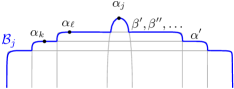
Figure 34: If $\alpha^{\prime},\beta^{\prime}\in\text{in}_{j}^{+}$, then $j<k<\ell$ and $(\alpha_{k},\alpha_{\ell},\alpha_{j},\beta^{\prime},\alpha^{\prime})$ appear in ccw order on $\mathcal{B}_{j}$.

Since many auxiliary arcs of $\text{in}_{j}^{+}$ can have the same source, we define

$$N_{j}=\{\text{source}_{j}(\alpha^{\prime})\in\mathscr{S}_{i}\;|\;\alpha^{\prime}\in\text{in}_{j}^{+}\}.$$

All arcs in $N_{j}$ are of different sites. Sets $\text{in}^{+}_{j}$ and $\text{in}^{+}_{k}$, $k\neq j$, may have many common arcs. However, we have the following disjointness property.

Lemma 19.

$N_{j}\cap N_{k}=\emptyset$ for all $k\neq j$. Thus, $\sum_{j=1}^{i}|N_{j}|=O(i)$.

Proof.

Suppose $\alpha_{\ell}\in N_{j}\cap N_{k}$ and $j<k$, then $\alpha_{\ell}=\text{source}_{j}(\alpha^{\prime})$, where $\alpha^{\prime}\in\text{in}^{+}_{j}$ and $\alpha_{\ell}=\text{source}_{k}(\alpha^{\prime\prime})$, where $\alpha^{\prime\prime}\in\text{in}^{+}_{k}$. (The arcs $\alpha^{\prime}$ and $\alpha^{\prime\prime}$ may or may not overlap). By Observation 3, $j<\ell$ (resp. $k<\ell$) and $(\alpha_{\ell},\alpha_{j},\alpha^{\prime})$ (resp. $(\alpha_{\ell},\alpha_{k},\alpha")$) must appear in ccw order on $\mathcal{B}_{j}$ (resp. $\mathcal{B}_{k}$).

Suppose first that $(\alpha_{\ell},\alpha_{k},\alpha_{j})$ appear in ccw order on $\mathcal{B}_{i}$. Then, since $k<\ell$, the arc $\alpha_{k}$ is inserted before $\alpha_{\ell}$ in $\mathcal{B}_{j}$, and thus, $\alpha^{\prime}$ cannot exist in $\mathcal{B}_{j}$, see Fig. 36. Suppose now that $(\alpha_{\ell},\alpha_{j},\alpha_{k})$ appear in ccw order on $\mathcal{B}_{i}$. Then, since $j<\ell$, the arc $\alpha_{j}$ is inserted before $\alpha_{\ell}$ in $\mathcal{B}_{k}$, thus, $\alpha^{\prime\prime}$ cannot exist on $\mathcal{B}_{k}$, see Fig. 36. In either case we derive a contradiction. ∎

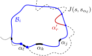
Figure 35: Illustration for Lemma 19. The case $(\alpha_{\ell},\alpha_{k},\alpha_{j})$ appear ccw.

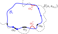
Figure 36: Illustration for Lemma 19. The case $(\alpha_{\ell},\alpha_{j},\alpha_{k})$ appear ccw.

We next establish that the parameters of the time complexity analysis for step $i$, as given in Definition 6 and Lemma 9, sum up to $O(i)$ on all boundary curves $\mathcal{B}_{j},j\leq i$.

Lemma 20.

Considering all the boundary curves of group $G(o_{i})$,

$$\sum_{j=1}^{i}(d_{1}(\alpha_{j},\mathcal{B}_{j})+d_{2}(\alpha_{j},\mathcal{B}_{j})+\tilde{d}(\alpha_{j},\mathcal{B}_{j}))=O(i).$$

Proof.

Let $\alpha$ and $\gamma$ denote the original arcs preceding and following $\alpha_{j}$ respectively in $\mathcal{B}_{i}$ (equiv. in $\mathcal{B}_{j}$). Let $d(\alpha_{j},\mathcal{B}_{k})$ denote the auxiliary arcs on the boundary curve $\mathcal{B}_{k}$, $k=i,j$, from $\alpha$ to $\gamma$.

We first observe that $d(\alpha_{j},\mathcal{B}_{j})$ cannot contain any portion of $\text{out}_{j}$ because no auxiliary arc of $\alpha_{j}$ may appear in $\mathcal{B}_{i}$ from $\alpha$ to $\gamma$, since $\alpha_{j}$ is the only core arc on $\mathcal{B}_{i}$ between $\alpha$ to $\gamma$. Thus, we only need to consider the auxiliary arcs of $\text{in}_{j}$. Next, we observe that no two auxiliary arcs in $d(\alpha_{j},\mathcal{B}_{j})$ can have the same source in $N_{j}$ for the same reason, i.e., there is no core arc from $\alpha$ to $\gamma$ except $\alpha_{j}$. Thus, we can bound $d(\alpha_{j},\mathcal{B}_{j})\leq d(\alpha_{j},\mathcal{B}_{i})+|N_{j}|$. Then, by Lemma 19, $\sum_{j=1}^{i}d(\alpha_{j},\mathcal{B}_{j})\leq|\mathcal{B}_{i}|+O(i)=O(i)$. Since $d_{1}(\alpha_{j},\mathcal{B}_{j})+d_{2}(\alpha_{j},\mathcal{B}_{j})\leq d(\alpha_{j},\mathcal{B}_{j})$, it follows $\sum_{j=1}^{i}(d_{1}(\alpha_{j},\mathcal{B}_{j})+d_{2}(\alpha_{j},\mathcal{B}_{j}))=O(i)$.

If $\tilde{d}(\alpha_{j},\mathcal{B}_{j})>0$, we have case (d) of Observation 1. In this case, the endpoints of $\alpha_{j}$ are incident to $\Gamma$, both in $\mathcal{B}_{j}$ and $\mathcal{B}_{i}$. Then, by Observations 2 and 4, both $\text{in}_{j}=\emptyset$ and $\text{out}_{j}=\emptyset$, implying that $\mathcal{B}_{j}=\mathcal{B}_{i}$; thus, $\tilde{d}(\alpha_{j},\mathcal{B}_{j})=\tilde{d}(\alpha_{j},\mathcal{B}_{i})$. Then, $\sum_{j=1}^{i}|\tilde{d}({\alpha_{j}},\mathcal{B}_{j})|\leq|\tilde{\mathcal{B}}_{i}|=O(i)$. ∎

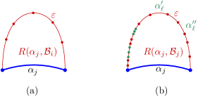
Figure 37: Illustration for Lemma 21. In between the two consecutively adjacent arcs $\alpha_{\ell}^{\prime}$ and $\alpha_{\ell}^{\prime\prime}$ of $\text{in}_{j}$ of the same source there must be an arc $\varepsilon\in\mathcal{B}_{i}$ that is adjacent to $R(\alpha_{j},\mathcal{B}_{j})$.

Lemma 21.

$|R(\alpha_{j},\mathcal{B}_{j})|\leq 2|R({\alpha_{j}},\mathcal{B}_{i})|+|N_{j}|$.

Proof.

We compare $R(\alpha_{j},\mathcal{B}_{j})$ and $R({\alpha_{j}},\mathcal{B}_{i})$ and bound differences in their adjacencies. First, we observe that no arc in $\text{out}_{j}$ can have a region adjacent to $R(\alpha_{j},\mathcal{B}_{j})$ (by Observation 2). Next, we observe that any arcs common to both $\mathcal{B}_{j}$ and $\mathcal{B}_{i}$, whose regions are adjacent to $R({\alpha_{j}},\mathcal{B}_{i})$, they must also be adjacent to $R({\alpha_{j}},\mathcal{B}_{j})$. In particular, if an arc $\varepsilon\in\mathcal{B}_{j}\cap\mathcal{B}_{i}$ has a region $R(\varepsilon,\mathcal{B}_{j})$ adjacent to $R(\alpha_{j},\mathcal{B}_{j})$ then $R(\varepsilon,\mathcal{B}_{i})$ must also be adjacent to $R({\alpha_{j}},\mathcal{B}_{i})$. This is clear, because otherwise, their common Voronoi edge $e$ in $\mathcal{V}_{l}(\mathcal{B}_{j})$ (or a portion of it) would be taken in $\mathcal{V}_{l}(\mathcal{B}_{i})$ by some arc in $\mathcal{B}_{i}$ that is missing from $\mathcal{B}_{j}$, by Lemma 17). This must be an auxiliary arc $\alpha_{j}^{\prime}$ of $\alpha_{j}$. But if we insert $\alpha_{j}^{\prime}$ to $\mathcal{V}_{l}(B_{j})$, the region $R(\alpha_{j}^{\prime},B_{j}\oplus\alpha_{j}^{\prime})$ will contain a portion of the edge $e$, thus, it will be adjacent to $R(\alpha_{j},B_{j}\oplus\alpha_{j}^{\prime})$, deriving a contradiction as arcs of the same site cannot be adjacent.

Let $|R(\alpha_{j},\mathcal{B}_{j})|_{x}$ denote the number of additional adjacencies that $R(\alpha_{j},\mathcal{B}_{j})$ may have over $R(\alpha_{j},\mathcal{B}_{i})$, i.e., $|R(\alpha_{j},\mathcal{B}_{j})|\leq|R(\alpha_{j},\mathcal{B}_{i})|+|R(\alpha_{j},\mathcal{B}_{j})|_{x}$. We show that $|R(\alpha_{j},\mathcal{B}_{j})|_{x}\leq|R(\alpha_{j},\mathcal{B}_{i})|+|N_{j}|$. Since auxiliary arcs of the same site can never have adjacent regions, it follows that between any two possible new adjacencies of $R(\alpha_{j},\mathcal{B}_{j})$ (counted in $|R(\alpha_{j},\mathcal{B}_{j})|_{x}$) with auxiliary arcs of $\text{in}_{j}$ belonging to the same source, there must be an adjacency with some arc not from $\text{in}_{j}$, which by the first paragraph is also contained in $\mathcal{B}_{i}$. Refer to Fig. 37(b), where in between the two consecutively adjacent arcs $\alpha_{\ell}^{\prime}$ and $\alpha_{\ell}^{\prime\prime}$ of $\text{in}_{j}$ the arc $\varepsilon\in\mathcal{B}_{i}$ is adjacent to $R(\alpha_{j},\mathcal{B}_{j})$.

Since by Observation 4 auxiliary arcs of one source in $N_{j}$ must appear in a certain order along $\mathcal{B}_{j}$ and they cannot alternate, the bound follows. ∎

Lemma 22.

Consider case (c) of Observation 1 at the insertion time of $\alpha_{j}$ in $\mathcal{B}_{j}$. Suppose that the insertion of $\alpha_{j}$ splits an existing arc $\omega$ into two pieces $\omega_{1}$ and $\omega_{2}$. Then at least one of these two arcs (say $\omega_{1}$) must also exist in $\mathcal{B}_{i}$. Further, $|R({\omega_{1}},\mathcal{B}_{j})|\leq 2|R({\omega_{1}},\mathcal{B}_{i})|+|N_{j}|$.

Proof.

Suppose $\omega_{1}\alpha_{j}\omega_{2}$ appear in $\mathcal{B}_{j}$ in ccw order and $\omega_{2}\not\in\mathcal{B}_{i}$. Then $\omega_{2}\in\text{in}_{j}^{+}$, see Fig. 38. Let $\alpha_{\ell}=\text{source}_{j}(\omega_{2})$, then $\ell>j$ as $\omega_{2}\in\text{in}_{j}^{+}$. We claim that $\omega_{1}$ must belong in $\mathcal{B}_{i}$.

Let $\tilde{\omega}\supset\alpha_{\ell}$ denote the expanded arc created at the insertion time of $\alpha_{\ell}$ following the order $o_{j}$. Clearly, $\tilde{\omega}\supset\omega$. Let $\hat{\omega}\supset\alpha_{\ell}$ denote the expanded arc created at the insertion time of $\alpha_{\ell}$, following $o_{i}$. Since $\ell>j$, it follows that $\hat{\omega}$ can extend ccw at most until $\alpha_{j}$ and $\hat{\omega}\subset\tilde{\omega}$. Since $\tilde{\omega}$ extends ccw past $\alpha_{j}$, it follows that no core arc $\alpha_{\rho}$, with $\rho<\ell$ can exist between $\alpha_{l}$ and $\alpha_{j}$. Thus, $\hat{\omega}$ must extend ccw to $\alpha_{j}$ and $\hat{\omega}\supset\omega_{1}$. In addition, no $\alpha_{\rho}$, with $\rho>\ell$, can delete $\omega_{1}$ during its insertion, while following $o_{i}$, because the same would happen in $o_{j}$ and $\omega_{1}$ exists in $\mathcal{B}_{j}$. Thus, $\omega_{1}$ must exist in $\mathcal{B}_{i}$.

We can now bound $|R({\omega_{1}},\mathcal{B}_{j})|\leq 2|R({\omega_{1}},\mathcal{B}_{i})|+|N_{j}|$ analogously to Lemma 21. The only additional argument needed for the fact that no arc in $\text{out}_{j}$ can have a region adjacent to $R(\omega_{1},\mathcal{B}_{j})$ is the observation that each arc in $\text{out}_{j}$ lies below the $s_{\omega}$-bisector, because arc $\alpha_{j}$ splits arc $\omega$ (case (c) of Observation 1). ∎

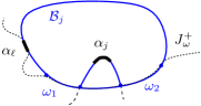
Figure 38: Illustration for the proof of Lemma 22. If $\omega_{2}\not\in\mathcal{B}_{i}$, then $\omega_{1}\in\mathcal{B}_{i}$.

Let $T(i,o_{j})$ denote the time that step-$i$ requires following permutation $o_{j}$, i.e., the time required by the last arc insertion of $o_{j}$.

Lemma 23.

The time for step-$i$ on the entire group $G=G(o_{i})$ is

$$T(i,G)=\sum_{o_{j}\in G}T(i,o_{j})=O(i)$$

Proof.

Lemmas 21 and 22 establish that $|R(\alpha_{j},\mathcal{B}_{j})|+|R(\omega_{j},\mathcal{B}_{j})|\leq 2(|R({\alpha_{j}},\mathcal{B}_{i})|+|R(\omega_{j},\mathcal{B}_{i})|+|N_{j}|)$, where $\omega_{j}$ denotes one of the two arcs that is split and belongs to $\mathcal{B}_{i}$ if case (c) of Observation 1 is concerned. Since $\omega_{j}$ is always an immediate neighbor of $\alpha_{j}$, we count it at most twice and thus, the total complexity $\sum_{j=1}^{i}|R(\omega_{j},\mathcal{B}_{i})|$ is $O(i)$. Together with Lemma 19 this directly implies that $\sum_{j=1}^{i}|R(\alpha_{j},\mathcal{B}_{j})|+r(\alpha_{j},\mathcal{B}_{j})=O(i)$. Lemma 20 establishes that $\sum_{j=1}^{i}d_{1}(\alpha_{j},\mathcal{B}_{j})+d_{2}(\alpha_{j},\mathcal{B}_{j})+\tilde{d}(\alpha_{j},\mathcal{B}_{j})=O(i)$. Then by Lemma 9 the claim is derived. ∎

Before stating the final result, we show that the partitioning of each block of $i!$ nodes (permutations) at level-$i$ of $\mathcal{T}$ into $(i-1)!$ groups of $i$ permutations each, is possible, if we follow the scheme we described in equation (2) for $G(o_{i})$. Let $\Pi_{i}$ denote such a block of all $i!$ permutations of the set $\mathscr{S}_{i}$. The references and the proof of the following lemma were provided by Stefan Felsner [9].

Lemma 24.

The partitioning of $\Pi_{i}$ into groups by the scheme we defined in equation (2) is possible, i.e.: For all $i\in\mathbb{N}$ and any block $\Pi_{i}$ of permutations on $\mathscr{S}_{i}$ there exists a set $F\subset\Pi_{i}$ of $(i-1)!$ permutations such that $\Pi_{i}=\dot{\bigcup}_{o\in F}G(o)$.

Proof.

Following [16] denote by $\left\lfloor\pi\right\rfloor$ the set of all permutations that are obtained from a permutation $\pi$ by deleting one element. The following property is clearly an equivalent condition for a set $F$ to satisfy $\Pi_{i}=\dot{\bigcup}_{o\in F}G(o)$. For each $\pi,\sigma\in F$ the sets $\left\lfloor\pi\right\rfloor$ and $\left\lfloor\sigma\right\rfloor$ are disjoint. Levenshtein calls a family $F$ of $(i-1)!$ permutations with this disjointness property a code capable of correcting single deletions and proves that these codes exist for all $i\in\mathbb{N}$ [16, Theorem 3.1]. ∎

All permutations at level-$i$ of the decision tree are equally likely. By Lemma 24, it is possible to partition them into groups of $i$ nodes each, which satisfy our scheme of equation (2). By Lemma 23, each group requires total $O(i)$ time to perform step $i$ on all its permutations. We thus conclude:

Theorem 4.

The expected time complexity of step $i$ of the randomized algorithm is $O(1)$.

We conclude with the following theorem.

Theorem 5.

Given an abstract Voronoi diagram $\mathcal{V}(S)$, $\mathcal{V}(S\setminus\{s\})\cap\mbox{VR}(s,S)$ can be computed in expected $O(h)$ time, where $h$ is the complexity of $\partial\mbox{VR}(s,S)$. Thus, $\mathcal{V}(S\setminus\{s\})$ can be updated from $\mathcal{V}(S)$ in expected time $O(h)$.

7 Computing the order-$k$ Voronoi diagram iteratively

Our algorithm to perform deletion in expected linear-time can be adapted to iteratively compute the order-${k}$ abstract Voronoi diagram, for increasing values of $k$, in total time $O(k(n-k)n+n\log n)$ if $k\leq n/2$. In particular, given a face $f$ of an order-$k$ Voronoi region, we can compute the order-$(k{+}1)$-subdivision within $f$ in expected time $O(|\partial f|)$. In this section we describe the required adaptation over site-deletion.

The order-$k$ abstract Voronoi region of a subset of sites $H\subset S$, $|H|=k$, is defined [3] as

$$\mbox{VR}_{k}{(}H,S)~{}=~{}\bigcap_{q\in H,p\in S\setminus H}D(q,p).$$

The order-$k$ abstract Voronoi diagram of $S$ is [3]

$$\mathcal{V}_{k}(S)=\mathbb{R}^{2}\setminus\bigcup_{H\subset S,|H|=k}\mbox{VR}_{k}{(}H,S).$$

The combinatorial complexity of $\mathcal{V}_{k}(S)$ is $O(k(n-k))$. For $k=1$, it is the nearest-neighbor abstract Voronoi diagram $\mathcal{V}(S)$, and for $k=n-1$, it is the farthest abstract Voronoi diagram $\mathrm{FVD}(S)$. The vertices of the diagram are classified into new and old, where a new vertex in $\mathcal{V}_{k}(S)$ is an old vertex of $\mathcal{V}_{k+1}(S)$.

Consider a face $f$ of an order-$k$ Voronoi region $\mbox{VR}_{k}{(}H)$, $H\subset S,|H|=k$. Let $S_{f}\subseteq S\setminus H$ denote the set of sites, which together with $H$, induce the Voronoi edges on the boundary $\partial f$. Our goal is to compute the Voronoi diagram of $S\setminus H$ within $f$, $\mathcal{V}(S_{f})\cap f$, in expected linear time, i.e., in time $O(|\partial f|)$. This diagram is a tree (or forest if $f$ is unbounded) with properties analogous to Lemma 1 (see also [5]). To extend Theorem 5 from $k=1$ to an arbitrary $k$, there is a non-trivial challenge to overcome: the complexity of $\partial f$ depends not only on $|S_{f}|$ but also on $k$. A direct application of our deletion algorithm would not result in a linear-time scheme for non-constant $k$.

Consider a face $f$ of $\mbox{VR}_{k}{(}H,S)$ and its boundary $\partial f$. We call any piece of $\partial f$ between two consecutive new vertices, an order-$k$ arc. Such an arc does not have constant complexity but may contain a sequence of old Voronoi vertices on $\partial f$. In this section, let $\mathscr{S}$ denote the collection of the order-$k$ arcs along the boundary of $f$.

An order-$k$ arc $\alpha$ is a piece of a so-called Hausdorff bisector between a site $s_{\alpha}\in S_{f}$ and $H$ (see, e.g., [19] for the definition of concrete Hausdorff bisectors and the Hausdorff Voronoi diagram of point-clusters). In abstract terms, the Hausdorff bisector between a site $s_{\alpha}\in S_{f}$ and $H$ can be defined as

$$J(s_{\alpha},H)=\partial\mbox{FVR}(s_{\alpha},H\cup\{s_{\alpha}\}),$$

where $\mbox{FVR}(s,S^{\prime})$ is the farthest Voronoi region of a site $s\in S^{\prime}\subseteq S$, $\mbox{FVR}(s,S^{\prime})=\bigcap_{q\in S^{\prime}\setminus\{s\}}D(q,s)$.

$J(s_{\alpha},H)$ is an unbounded Jordan curve dividing the plane in two parts; let $D(s_{\alpha},H)=\mbox{FVR}(s_{\alpha},H\cup\{s_{\alpha}\})$. The complexity of $J(s_{\alpha},H)$ is $\Theta(|H|)$, and this is an obstacle in directly applying our randomized linear time scheme. It is possible to overcome this problem by considering relaxed Hausdorff bisectors whose complexity depends solely on the order-$k$ arc, and which define a series of even larger shrinking domains enclosing the face $f$.

Let $H_{\alpha}\subseteq H$ be the subset of sites in $H$ that, together with $s_{\alpha}$, define the edges and vertices along the arc $\alpha$. Instead of $J(s_{\alpha},H)$, which is hard to compute, we consider the Hausdorff bisector $J(s_{\alpha},H_{\alpha})$, where $\alpha\subseteq J(s_{\alpha},H_{\alpha})$, and has complexity $\Theta(|H_{\alpha}|)$. In fact, $\alpha\subseteq J(s_{\alpha},\tilde{H}_{\alpha})$, for any $H_{\alpha}\subseteq\tilde{H}_{\alpha}\subseteq H$. Let $|\alpha|$ denote the complexity of arc $\alpha$, $|\alpha|=|H_{\alpha}|$. We make use of the following property.

Lemma 25.

$J(s_{\alpha},H)\subseteq\overline{D(s_{\alpha},\tilde{H}_{\alpha})}\subseteq\overline{D(s_{\alpha},H_{\alpha})}$, where $H_{\alpha}\subseteq\tilde{H}_{\alpha}\subseteq H$.

Proof.

Since $H_{\alpha}\subseteq H$, we have

$$D(s_{\alpha},H)=\mbox{FVR}(s_{\alpha},H\cup\{s_{\alpha}\})\subseteq\mbox{FVR}(s_{\alpha},H_{\alpha}\cup\{s_{\alpha}\})=D(s_{\alpha},H_{\alpha}).$$ (3)

Thus, it holds $J(s_{\alpha},H)=\partial{D(s_{\alpha},H)}\subseteq\overline{D(s_{\alpha},H_{\alpha})}$. Analogously we can show the subset relation for $\tilde{H}_{\alpha}$. ∎

It is now straightforward to adapt the algorithm of Section 6, using appropriate Hausdorff bisectors that are derived by the order-$k$ arcs in $\mathscr{S}$, in place of the $s$-related bisectors in the previous sections. The complexity of each such Hausdorff bisector must be proportional to the complexity of its underlying order-$k$ arc. Lemma 25 implies the correctness of adopting this relaxation.

We start with domain $D_{1}$ defined by $J(s_{\alpha_{1}},H_{\alpha_{1}})$, i.e., $D_{1}=D(s_{\alpha_{1}},H_{\alpha_{1}})\cap D_{\Gamma}$, for the first order-$k$ arc $\alpha_{1}$ of a random permutation of $\mathscr{S}$. The boundary complexity of $D_{1}$ is $O(|\alpha_{1}|)$. Note that $D_{1}$ is a superset of domain $D(s_{\alpha_{1}},H)\cap D_{\Gamma}$. At step $i$, we insert arc $\alpha_{i}$ considering bisector $J(s_{\alpha_{i}},\tilde{H}_{\alpha_{i}})$, where $H\supseteq\tilde{H}_{\alpha_{i}}\supseteq H_{\alpha_{i}}$, and $|\tilde{H}_{\alpha_{i}}|\leq|H_{\alpha_{i}}|+2$. We use $\tilde{H}_{\alpha_{i}}$, possibly a superset of $H_{\alpha_{i}}$, in order to include at most one site in $H$ for each neighbor of $\alpha_{i}$ in $\mathcal{P}_{i}$. This is done to correctly link two neighboring order-$k$ arcs on $\mathcal{P}_{i}$ so that they are both incident to a common (new) Voronoi vertex. By Lemma 25, domain $D_{i}$ is a superset of the domain we would get if we instead considered bisector $J(s_{\alpha_{i}},H)\supset\alpha_{i}$. Therefore, the relaxed construction works correctly. At the end, $D_{h}=f$.

We conclude that Theorem 5 applies, constructing $\mathcal{V}(\mathscr{S})=\mathcal{V}(S_{f})\cap f$ in expected time $O(|\partial f|)$.

Since the complexity of $\mathcal{V}_{k}(S)$ is $O(k(n-k))$, the $O(k^{2}(n-k)+n\log n)$ bound for iteratively constructing the diagram, starting at $\mathcal{V}(S)$, easily follows for $k\leq n/2$. Although there are algorithms of better time-complexity to construct $\mathcal{V}_{k}(S)$, such as the $O(k(n-k)\log^{2}n+n\log^{3}n)$ randomized incremental algorithm of Bohler et al. [5], the iterative construction is nice and simple, therefore, it can be preferable for small values of $k$.

8 The farthest abstract Voronoi diagram

In this section we show how to modify (in fact simplify) the algorithm for the deletion of one site to compute the farthest abstract Voronoi diagram, after the sequence of its faces at infinity is known.

The farthest Voronoi region of a site $p\in S$ is $\mbox{FVR}(p,S)=\bigcap_{q\in S\setminus\{p\}}D(q,p)$ and the farthest abstract Voronoi diagram of $S$ is $\mathrm{FVD}(S)=\mathbb{R}^{2}\setminus\bigcup_{p\in S}\mbox{FVR}(p,S)$. $\mathrm{FVD}(S)$ is a tree of complexity $O(n)$, however, regions may be disconnected and a farthest Voronoi region may consist of $\Theta(n)$ disjoint faces [17]. Let $D^{*}(p,q)=D(q,p)$; then $\mbox{FVR}(p,S)=\bigcap_{q\in S\setminus\{p\}}D^{*}(p,q)$.

Unless otherwise noted, we adopt the following convention: we reverse the labels of bisectors and use $D^{*}(\cdot,\cdot)$, in the place of $D(\cdot,\cdot)$, in most definitions and constructs of Sections 3, 4. Under this convention the definition of e.g., a $p$-monotone path remains the same but it uses $\partial\mbox{FVR}(p,\cdot)$ in the place of $\partial\mbox{VR}(p,\cdot)$. The corresponding arrangement of $p$-related bisectors $\mathcal{J}_{p,S^{\prime}}$, $S^{\prime}\subseteq S$, is considered with the labels of bisectors and their dominance regions reversed from the original system $\mathcal{J}$.

Consider the enclosing curve $\Gamma$ as defined in Section 2, and let $\mathscr{S}$ be the sequence of arcs on $\Gamma$ derived by $\Gamma\cap\mathrm{FVD}(S)$. $\mathscr{S}$ represents the sequence of the farthest Voronoi faces in $\mathrm{FVD}(S)$ at infinity. The domain of computation is $D_{\Gamma}$. For an arc $\alpha$ of $\mathscr{S}$, let $s_{\alpha}$ denote the site in $S$ for which $\alpha\subset\mbox{FVR}(s_{\alpha},S)$. With respect to site occurrences, $\mathscr{S}$ is a Davenport-Schinzel sequence of order 2. $\mathscr{S}$ can be computed in time $O(n\log n)$ in a divide and conquer fashion, similarly to computing the hull of a farthest segment Voronoi diagram, see e.g., [20].

We treat the arcs in $\mathscr{S}$ as sites and compute $\mathcal{V}(\mathscr{S})=\mathrm{FVD}(S)\cap D_{\Gamma}$. Let $\text{VR}(\alpha,\mathscr{S})$ denote the face of $\mathrm{FVD}(S)\cap D_{\Gamma}$ incident to $\alpha\in\mathscr{S}$, see Fig. 39. $\mathcal{V}(\mathscr{S})$ is a tree whose leaves are the endpoints of the arcs in $\mathscr{S}$.

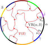
Figure 39: The farthest Voronoi diagram $\mathcal{V}(\mathscr{S})=\mathrm{FVD}(S)\cap D_{\Gamma}$ and the Voronoi region $\mbox{VR}(\alpha,\mathscr{S})$. Bisector labels are shown in the farthest (reversed) sense.

Consider $\mathscr{S}^{\prime}\subseteq\mathscr{S}$, and let $S^{\prime}\subseteq S$ be the set of sites that define the arcs in $\mathscr{S}^{\prime}$. Let $\mathcal{J}(S^{\prime})=\{J(p,q)\in\mathcal{J}\,|\,p,q\in S^{\prime},p\neq q\}$.

Definition 8.

A boundary curve $\mathcal{P}$ for $\mathscr{S}^{\prime}$ is a partitioning of $\Gamma$ into arcs whose endpoints are in $\Gamma\cap\mathcal{J}(S^{\prime})$ such that any two consecutive arcs $\alpha,\beta\in\mathcal{P}$ are incident to $J(s_{\alpha},s_{\beta})\in\mathcal{J}(S^{\prime})$, having consistent labels, and $\mathcal{P}$ contains an arc $\alpha\supseteq\alpha^{*}$, for every core arc $\alpha^{*}\in\mathscr{S}^{\prime}$. We say that the labels of $\alpha$, $\beta$ are consistent, if there is a neighborhood $\tilde{\alpha}\subseteq\alpha$ and $\tilde{\beta}\subseteq\beta$ incident to the common endpoint of $\alpha$ and $\beta$ such that $\tilde{\alpha}\in D^{*}(s_{\alpha},s_{\beta})$, and $\tilde{\beta}\in D^{*}(s_{\beta},s_{\alpha})$.

There can be several different boundary curves for $\mathscr{S}^{\prime}$. The arcs in $\mathcal{P}$ that contain a core arc in $\mathscr{S}^{\prime}$ are called original and any remaining arcs are called auxiliary. The arcs in $\mathcal{P}$, although they are arcs on $\Gamma$, they are all boundary arcs and none is considered a $\Gamma$-arc in the sense of the previous sections. The endpoint $J(s_{\alpha},s_{\beta})\cap\Gamma$ on $\mathcal{P}$ separating two consecutive arcs $\alpha,\beta$ is denoted by $\nu(\alpha,\beta)$.

The Voronoi-like diagram of a boundary curve $\mathcal{P}$ is defined analogously to Definition 4. Since $\mathcal{P}$ consists only of boundary arcs, $\mathcal{V}_{l}(\mathcal{P})$ is a tree whose leaves are the vertices of $\mathcal{P}$. The properties of a Voronoi-like diagram in Section 3 remain the same (under the conventions of this section).

Given $\mathcal{V}_{l}(\mathcal{P})$ for a boundary curve $\mathcal{P}$ of $\mathscr{S}^{\prime}\subset\mathscr{S}$, we can insert a core arc $\beta^{*}\in\mathscr{S}\setminus\mathscr{S}^{\prime}$ and obtain $\mathcal{V}_{l}(\mathcal{P}\oplus\beta^{*})$. The insertion is performed analogously to Section 4. The original arc $\beta\supseteq\beta^{*}$, with endpoints $x,y$ is defined as follows: let $\delta$ be the first arc on $\mathcal{P}$ counterclockwise (resp. clockwise) from $\beta^{*}$ such that $J(s_{\beta},s_{\delta})\cap\delta\neq\emptyset$; let $x=\nu(\delta,\beta)$ (resp. $y=\nu(\beta,\delta)$). Let $\mathcal{P}_{\beta}=\mathcal{P}\oplus\beta$ be the boundary curve obtained from $\mathcal{P}$ by substituting with $\beta$ its overlapping piece from $x$ to $y$. No original arc of $\mathcal{P}$ can be deleted by the insertion of $\beta$. Observation 1 remains the same, except from cases (d),(e) that do not exist.

The merge curve $J(\beta)$, given $\mathcal{V}_{l}(\mathcal{P})$, is defined analogously to Definition 5; it is only simpler as it does not contain $\Gamma$-arcs. Theorem 2 remains valid, i.e., $J(\beta)$ is an $s_{\beta}$-monotone path in $\mathcal{J}_{s_{\beta},S^{\prime}}$ connecting the endpoints of $\beta$. The proof structure is the same as for Theorem 2, however, Lemma 13 now requires a different proof, which we give in the sequel (see Lemma 27). Lemma 14 is not relevant; while Lemma 15 and Lemma 16 are analogous.

In the following lemma we restore the labeling of bisectors to the original.

Lemma 26.

In an admissible bisector system $\mathcal{J}$ (or $\mathcal{J}\cup\Gamma$) there cannot be two $p$-cycles, $p\in S$, with disjoint interior.

Proof.

By its definition, the nearest Voronoi region $\mbox{VR}(p,S)$ (resp. $\mbox{VR}(p,S)\cap D_{\Gamma}$) must be enclosed in the interior of any $p$-cycle of the admissible bisector system $\mathcal{J}$ (resp. $\mathcal{J}\cup\Gamma$). But $\mbox{VR}(p,S)$ (resp. $\mbox{VR}(p,S)\cap D_{\Gamma}$) is connected (by axiom (A1)), thus, there cannot be two different $p$-cycles with disjoint interior. ∎

Lemma 27.

Consider the merge curve $J(\beta)$. Suppose $v_{i+1}$ is not a valid vertex because $v_{i+1}\in\alpha_{i}$, i.e., $e_{i}$ hits arc $\alpha_{i}$. Then vertex $v_{m-j}$ can not be on $\mathcal{P}$.

Proof.

Suppose otherwise, i.e., vertex $v_{m-j}$ is on the boundary arc $\alpha_{m-j}$. Then $J_{x}^{i}$ and $J_{y}^{j}$ partition $D_{\Gamma}$ in three parts: a middle part incident to $\beta$, and two parts $C_{1}$ and $C_{2}$ at either side of $J_{x}^{i}$ and $J_{y}^{j}$ respectively, whose closures are disjoint, see Fig. 40. But the boundaries of $C_{1}$ and $C_{2}$ are $s_{\beta}$-cycles in the admissible bisector system $\mathcal{J}\cup\Gamma$ contradicting Lemma 26. Note that here we use the original labels of bisectors, including $\Gamma=J(s_{\beta},s_{\infty})$. ∎

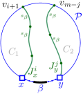
Figure 40: Illustration for Lemma 27. Nearest labels are shown.

The diagram ${\mathcal{V}_{l}(\mathcal{P})\oplus\beta}$ is defined analogously and the proof that ${\mathcal{V}_{l}(\mathcal{P})\oplus\beta}$ is the Voronoi-like diagram $\mathcal{V}_{l}(\mathcal{P}_{\beta})$ for $\mathcal{P}_{\beta}=\mathcal{P}\oplus\beta$, is analogous to the proof of Theorem 3.

The randomized algorithm for computing $\mathcal{V}(\mathscr{S})=\mathrm{FVD}(S)\cap D_{\Gamma}$ is the same as in Section 6. The time analysis is also completely analogous. For completeness we point out that, here, the set $\text{out}_{j}$ consists of the auxiliary arcs in $\mathcal{B}_{j}$ that overlap with the auxiliary arcs of $\alpha_{j}$ in $\mathcal{B}_{i}$. The set $\text{in}_{j}$ are any remaining auxiliary arcs in $\mathcal{B}_{j}\setminus\text{out}_{j}$ that differ from the corresponding auxiliary arcs in $\mathcal{B}_{i}$. All observations of Section 6.1 remain intact under this updated notion of $\text{in}_{j}$ and $\text{out}_{j}$. Thus, the (expected) linear time complexity can be analogously established.

Theorem 6.

Given the sequence of its faces at infinity, i.e., given the sequence of arcs $\mathscr{S}$ implied by $\mathrm{FVD}(S)\cap\Gamma$, the farthest abstract Voronoi diagram $\mathrm{FVD}(S)$ can be computed in expected linear time $O(|\mathscr{S}|)$.

9 Concluding remarks

In this paper we formalized the notion of an abstract Voronoi-like diagram, which is defined as a graph (tree or forest) on the arrangement of the underlying bisector system whose vertices are legal Voronoi vertices in Voronoi diagrams of three sites. We defined the Voronoi-like diagram of a boundary curve, which is implied by a subset $\mathscr{S}^{\prime}$ of Voronoi edges bounding a Voronoi region $\mbox{VR}(s,S)$. A boundary curve is defined as an $s$-monotone path in the arrangement of $s$-related bisectors that contains the arcs in $\mathscr{S}^{\prime}$. We showed that the Voronoi-like diagram of such a boundary curve is well-defined, unique, and robust under an arc-insertion operation, which enables its use in incremental constructions. Using Voronoi-like diagrams as intermediate structures, we derived a very simple, therefore practical, randomized incremental algorithm to update an abstract Voronoi diagram after deletion of one site in expected linear time. The algorithm is applicable to any concrete diagram under the umbrella of abstract Voronoi diagrams.

The technique can be adapted to compute the order-$(k{+}1)$ subdivision within an order-$k$ abstract Voronoi region, and the farthest abstract Voronoi diagram, after the order of its faces at infinity is known. The Voronoi-like structure provides the means to efficiently deal with the underlying disconnected Voronoi regions, which is the common complication characterizing these simple tree (or forest) Voronoi structures.

A deterministic linear-time construction for these problems has remained an open problem. In future research, we would like to investigate the applicability of the Voronoi-like structure within the linear-time framework of Aggarwal et al. [1] aiming to a deterministic linear-time algorithm for the same problems.

References

- [1] Alok Aggarwal, Leonidas J. Guibas, James B. Saxe, and Peter W. Shor. A linear-time algorithm for computing the voronoi diagram of a convex polygon. Discrete & Computational Geometry, 4:591–604, 1989.
- [2] Franz Aurenhammer, Rolf Klein, and Der-Tsai Lee. Voronoi Diagrams and Delaunay Triangulations. World Scientific, 2013.
- [3] Cecilia Bohler, Panagiotis Cheilaris, Rolf Klein, Chih-Hung Liu, Evanthia Papadopoulou, and Maksym Zavershynskyi. On the complexity of higher order abstract Voronoi diagrams. Computational Geometry: Theory and Applications, 48(8):539–551, 2015.
- [4] Cecilia Bohler, Rolf Klein, Andrzej Lingas, and Chih-Hung Liu. Forest-like abstract voronoi diagrams in linear time. Computational Geometry, 68:134 – 145, 2018.
- [5] Cecilia Bohler, Rolf Klein, and Chih-Hung Liu. An efficient randomized algorithm for higher-order abstract voronoi diagrams. Algorithmica, 81(6):2317–2345, 2019.
- [6] Kevin Buchin, Olivier Devillers, Wolfgang Mulzer, Okke Schrijvers, and Jonathan Shewchuk. Vertex deletion for 3D Delaunay triangulations. In Algorithms – ESA 2013, volume 8125 of LNCS, pages 253–264, Berlin, Heidelberg, 2013. Springer Berlin Heidelberg.
- [7] Paul L. Chew. Building Voronoi diagrams for convex polygons in linear expected time. Technical report, Dartmouth College, Hanover, USA, 1990.
- [8] Francis Chin, Jack Snoeyink, and Cao An Wang. Finding the medial axis of a simple polygon in linear time. Discrete & Computational Geometry, 21(3):405–420, 1999.
- [9] Stefan Felsner. Personal communication, 2019.
- [10] Kolja Junginger and Evanthia Papadopoulou. Deletion in Abstract Voronoi Diagrams in Expected Linear Time. In 34th International Symposium on Computational Geometry (SoCG 2018), volume 99 of LIPIcs, pages 50:1–50:14, Dagstuhl, Germany, 2018.
- [11] Elena Khramtcova and Evanthia Papadopoulou. An expected linear-time algorithm for the farthest-segment Voronoi diagram. arXiv:1411.2816v3 [cs.CG], 2017. Preliminary version in Proc. 26th Int. Symp. on Algorithms and Computation (ISAAC), LNCS 9472, 404-414, 2015.
- [12] Rolf Klein. Concrete and Abstract Voronoi Diagrams, volume 400 of Lecture Notes in Computer Science. Springer-Verlag, 1989.
- [13] Rolf Klein, Elmar Langetepe, and Z. Nilforoushan. Abstract Voronoi diagrams revisited. Computational Geometry: Theory and Applications, 42(9):885–902, 2009.
- [14] Rolf Klein and Andrzej Lingas. Hamiltonian abstract Voronoi diagrams in linear time. In Algorithms and Computation, 5th International Symposium, (ISAAC), volume 834 of Lecture Notes in Computer Science, pages 11–19, 1994.
- [15] Rolf Klein, Kurt Mehlhorn, and Stefan Meiser. Randomized incremental construction of abstract Voronoi diagrams. Computational geometry: Theory and Applications, 3:157–184, 1993.
- [16] Vladimir Levenshtein. On perfect codes in deletion and insertion metric. Discrete Mathematics and Applications, 2(3):241–258, 1992.
- [17] K. Mehlhorn, S. Meiser, and R. Rasch. Furthest site abstract Voronoi diagrams. International Journal of Computational Geometry and Applications, 11(6):583–616, 2001.
- [18] Atsuyuki Okabe, Barry Boots, Kokichi Sugihara, and Sung Nok Chiu. Spatial Tessellations: Concepts and Applications of Voronoi Diagrams. John Wiley, second edition, 2000.
- [19] Evanthia Papadopoulou. The Hausdorff Voronoi diagram of point clusters in the plane. Algorithmica, 40:63–82, 2004.
- [20] Evanthia Papadopoulou and Sandeep K. Dey. On the farthest line-segment Voronoi diagram. International Journal of Computational Geometry and Applications, 23(6):443–459, 2013.
- [21] Micha Sharir and Pankaj K. Agarwal. Davenport-Schinzel sequences and their geometric applications. Cambridge university press, 1995.