A Switched Systems Approach to Path Following with Intermittent State Feedback

Abstract

Autonomous agents are often tasked with operating in an area where feedback is unavailable. Inspired by such applications, this paper develops a novel switched systems-based control method for uncertain nonlinear systems with temporary loss of state feedback. To compensate for intermittent feedback, an observer is used while state feedback is available to reduce the estimation error, and a predictor is utilized to propagate the estimates while state feedback is unavailable. Based on the resulting subsystems, maximum and minimum dwell time conditions are developed via a Lyapunov-based switched systems analysis to relax the constraint of maintaining constant feedback. Using the dwell time conditions, a switching trajectory is developed to enter and exit the feedback denied region in a manner that ensures the overall switched system remains stable. A scheme for designing a switching trajectory with a smooth transition function is provided. Simulation and experimental results are presented to demonstrate the performance of control design.

I Introduction

Acquiring state feedback is at the core of ensuring stability in control designs. However, factors such as the task definition, operating environment, or sensor modality can result in temporary loss of feedback. For example, agents may be required to limit communication during predefined time frames or when traversing through certain regions. Motivated by such factors, various path planning and control methods have been developed that seek to ensure uninterrupted feedback (cf., [1, 2, 3, 4, 5, 6, 7, 8, 9, 10, 11, 12]). Such results inherently constrain the trajectory or behavior of a system. For instance, visual servoing applications for nonholonomic systems can result in limited, sharp-angled or non-smooth trajectories to keep a target in the camera field-of-view (FOV) as illustrated in results such as [13, 14, 15]. Rather than trying to constrain the system to ensure continuous feedback is available, the approach in this paper leverages switched systems methods to achieve an objective despite intermittent feedback.

Solutions to relaxing the constant feedback constraint have been investigated. For example, methods to relax the requirement of keeping landmarks in the FOV have been developed in results such as [16] and [17]. In [16], multiple landmarks are linked together by a daisy-chaining approach where new landmarks are mapped onto the initial world frame and are used to provide state feedback when initial landmarks leave the FOV. Similar concepts were adopted in [17], where a wheeled mobile robot (WMR) is allowed to navigate around a landmark without constantly keeping it in the FOV by relating feature points in the background to the landmark and thus provide state feedback. Although the objective to eliminate the requirement of constant visual on the landmark is achieved, state feedback is assumed to be available during periods when the landmark is outside the FOV. Such daisy-chaining approaches provide state feedback in an ideal scenario, but the accuracy of the feedback may degrade or even diverge in the presence of measurement noise and disturbances in the dynamics.

Conventional approaches to the simultaneous localization and mapping (SLAM) problem, such as the works in [18, 19, 20], use relationships between features or landmarks to estimate the pose (i.e., position and orientation) of the sensor, usually a monocular camera, and simultaneously determine the position of landmarks with respect to the world frame. Typically, a feature rich environment with sufficient measurements are required for SLAM methods to provide state estimation. However, a well-known drawback with SLAM algorithms is that without proper loop closures the estimates will drift over time due to the accumulation of measurement noise (cf., [21, 22]). In this paper, a state estimate dynamic model propagates the state estimate when feedback is not available, and no additional feedback information is required. Sufficient conditions may be derived via a Lyapunov-based analysis to ensure the loop closures are achieved before the state estimates degrade beyond a desired threshold.

Stability of systems that experience random state feedback has been analyzed in previous literature. Typically, the intermittent loss of measurement is modeled as a random Bernoulli process with a known probability. Resulting trajectories are then analyzed in a probabilistic sense, where the expected value of the estimation error is shown to converge asymptotically, compared to the result in this paper which examines the behavior of the actual tracking and estimation errors.

The networked control systems (NCS) community has also examined systems with temporarily unavailable measurements. Results such as [23, 24, 25, 26] rely on a decision maker that is independent of the estimator or controller to determine when to broadcast sensor information. The objective in these results is to minimize the cost of network bandwidth by reducing the frequency of data transmission. In [27, 28, 29], data loss is modeled as random missing outputs and noisy measurements. In each case, state estimates are propagated by a model of the controlled system during the periods when transmission is missing. On the contrary, the availability of sensor information in this paper is not controlled by a decision maker but instead determined by the region in which the actual states are located. Therefore, sensor information is only available when the states are inside a feedback region.

It is well known that slow switching between stable subsystems may result in instability as explained in [30]. For slow switching between stable subsystems, the underlying strategy for proving stability involves developing switching conditions to ensure the overall system is stable. If a common Lyapunov function exists for all subsystems such that the time derivative of the Lyapunov function is upper bounded by a common negative definite function, the overall system is proven to be stable in [30]. For cases where a common Lyapunov function cannot be determined, multiple subsystem-specific Lyapunov functions are used. In general, the overall Lyapunov function is discontinuous and jumps may occur at switching interfaces. Therefore, the stability of such a system is achieved by placing switching conditions on the subsystems to enforce a decrease in the subsystem-specific Lyapunov functions between each successive activation of the respective subsystems. Typically, these requirements manifest as (average) dwell time conditions which specifies the duration for which each subsystem must remain active, as described in [30].

When a subset of the subsystems is unstable, a layer of complication is introduced to the analysis. A stability analysis is provided in [31] for switched systems with stable and unstable linear time invariant (LTI) subsystems, where an average dwell time condition is developed. Similarly, the authors in [32] developed dwell time conditions for nonlinear switched systems with exponentially stable and unstable subsystems. However, dwell time conditions typically require the stable subsystems to be activated longer than the unstable subsystems, as indicated in [31]. In [33], the authors developed an observer to estimate the depths of feature points in a image from a monocular camera and use a predictor to propagate the state estimates when the features are occluded or outside the FOV. Based on the error system formulation, the subsystem for the observer is stable, while the subsystem for the predictor is unstable. An average dwell time condition is developed to ensure the stability of the switched system. However, the focus of [33] is the estimation of feature depths and therefore have not focused on achieving a control objective when feedback is unavailable.

The development in this paper aims to achieve a path following objective despite intermittent loss of feedback. The novelty of this result is guaranteeing the stability of following a path which lies outside a region with feedback while maximizing the amount of time the agent spends in the feedback-denied environment. Switched systems methods are used to develop a state estimator and predictor when state feedback is available or not, respectively. Since switching occurs between a stable subsystem when feedback is available and an unstable subsystem when feedback is not available, dwell time conditions are developed that determine the minimum time that the agent must be in the feedback region versus the maximum time the agent can be in the feedback denied region. Using these dwell time conditions, a switching trajectory is designed based on the dwell time conditions that leads the agent in and out of the feedback denied region so that the overall system remains stable. The most similar result to this paper is in [34], which includes state prediction and control for a nonholonomic system moving around an obstacle. The goal in [34] is to regulate a nonholonomic vehicle to a set-point in the presence of intermittent feedback. However, the difficulty of path following in the current paper arises when the system is outside the feedback region.

The paper is organized as follows. In Section II, the system model is introduced. In Section III, the tracking and estimation objective is given and the respective error systems are defined. Based on the error dynamics, a Lyapunov-based stability analysis for the resulting switched system is performed in Section V to develop the dwell time conditions and to show stability of the overall system. In Section VI, a strategy for designing a switching trajectory is presented. A simulation is provided in Section VII and an experiment is provided in Section VIII to demonstrate the performance of the approach.

II System Model

Consider a dynamic system subject to an exogenous disturbance as

$$\dot{x}(t)=f(x(t),t)+v(t)+d(t),$$ (1)

where $x(t),\>\dot{x}(t)\in\mathbb{R}^{n}$ denote a generalized state and its time derivative, $f:\>\mathbb{R}^{n}\times\mathbb{R}\rightarrow\mathbb{R}^{n}$ denotes the locally Lipschitz drift dynamics, $v(t)\in\mathbb{R}^{n}$ is the control input, and $d(t)\in\mathbb{R}^{n}$ is the exogenous disturbance where the Euclidean norm is bounded as $\|d(t)\|\leq\bar{d}\in\mathbb{R}_{\geq 0}$ with $n\in\mathbb{N}$ and $t\in\mathbb{R}_{\geq 0}$.

III State Estimate and Control Objective

In this paper, the overall objective is to achieve path following under intermittent loss of feedback. Specifically, a known feedback region is denoted as a closed set $\mathcal{F}\subset\mathbb{R}^{n}$, where the complement region where feedback is unavailable is denoted by $\mathcal{F}^{c}$. That is, feedback is available when $x(t)\in\mathcal{F}$ and unavailable when $x(t)\in\mathcal{F}^{c}$.

A desired path is denoted as $x_{d}\subset\mathcal{F}^{c}$. It is clear that state feedback is unavailable while attempting to follow $x_{d}$, and hence the system must return to the feedback region $\mathcal{F}$ intermittently to maintain stability. Therefore, a switching trajectory, denoted by $\bar{x}_{d}(t)\in\mathbb{R}^{n}$, is designed to overlay $x_{d}$ as much as possible while adhering to the subsequently developed dwell time constraints. To quantify the ability of the controller to track the switching trajectory, the tracking error $e(t)\in\mathbb{R}^{n}$ is defined as

$$e(t) \triangleq e_{1}(t)+e_{2}(t),$$ (2)

where the estimate tracking error $e_{1}(t)\in\mathbb{R}^{n}$ is defined as

$$e_{1}(t) \triangleq \hat{x}(t)-\bar{x}_{d}(t),$$ (3)

and the state estimation error $e_{2}(t)\in\mathbb{R}^{n}$ is defined as

$$e_{2}(t) \triangleq x(t)-\hat{x}(t),$$ (4)

where $\hat{x}(t)\in\mathbb{R}^{n}$ is the state estimate.

Based on (3) and (4), the control objective is to ensure that $e_{1}(t)$ and $e_{2}(t)$ converge, and therefore $e(t)$ will converge. To facilitate the subsequent development, let the composite error vector be defined as $z(t)\triangleq\left[\begin{array}[]{cc}e_{1}^{T}(t)&e_{2}^{T}(t)\end{array}\right]^{T}$.

IV Controller and Update Law Design

To facilitate the subsequent analysis, two subsystems are defined to indicate when the states are inside or outside the feedback region. When $x(t)\in\mathcal{F}$, an exponentially stable observer can be designed using various approaches (e.g., observers such as [33, 35, 36] could be used). The subsequent development is based on an observer update law designed as

$$\dot{\hat{x}}(t)=f(\hat{x}(t),t)+v(t)+v_{r}(t),$$ (5)

where $v_{r}(t)\in\mathbb{R}^{n}$ is a high-frequency sliding-mode term designed as

$$v_{r}(t)=k_{2}e_{2}(t)+\bar{d}sgn(e_{2}(t)),$$ (6)

where $k_{2}\in\mathbb{R}^{n\times n}$ is a constant, positive definite gain matrix. When $x(t)\in\mathcal{F}^{c}$, the state estimate is updated by a predictor designed as

$$\dot{\hat{x}}(t)=f(\hat{x}(t),t)+v(t).$$ (7)

Since the state is required to transition between $\mathcal{F}$ and $\mathcal{F}^{c}$, a switched systems analysis is used to investigate the stability of the overall switched system. To facilitate this analysis, the error systems for $e_{1}(t)$ and $e_{2}(t)$ are expressed as

$$\dot{e}_{1}(t) =f_{1p}\left(\bar{x}_{d}(t),\hat{x}(t),t\right),$$ (8)

$$\dot{e}_{2}(t) =f_{2p}\left(x(t),\hat{x}(t),t\right),$$ (9)

where $f_{1p},\ f_{2p}:\mathbb{R}^{n}\times\mathbb{R}^{n}\times\mathbb{R}_{\geq 0}\rightarrow\mathbb{R}^{n},\;p\in\{a,u\}$, $a$ is an index for subsystems with available feedback, and $u$ is an index for subsystems when feedback is unavailable. Based on (8) and the subsequent stability analysis, the controller is designed as

$$v(t)=\begin{cases}\dot{\bar{x}}_{d}(t)-f(\hat{x}(t),t)-k_{1}e_{1}(t)-v_{r}(t),&p=a,\\ \dot{\bar{x}}_{d}(t)-f(\hat{x}(t),t)-k_{1}e_{1}(t),&p=u,\end{cases}$$ (10)

where $\dot{\bar{x}}_{d}(t)\in\mathbb{R}^{n}$, and $k_{1}\in\mathbb{R}^{n\times n}$ is a constant, positive definite gain matrix. By taking the time derivative of (3) and substituting (5), (7) and (10) into the resulting expression, (8) can be expressed as

$$\dot{e}_{1}(t)=-k_{1}e_{1}(t),\ \forall p.$$ (11)

After taking the time derivative of (4) and substituting (1), (5) and (7) into the resulting expression, the family of systems in (9) can be expressed as

$$\dot{e}_{2}(t)=\begin{cases}f(x(t),t)-f(\hat{x}(t),t)+d(t)\\ -\bar{d}sgn(e_{2}(t))-k_{2}e_{2}(t),&p=a,\\ f(x(t),t)-f(\hat{x}(t),t)+d(t),&p=u.\end{cases}$$ (12)

V Switched System Analysis

To further facilitate the analysis for the switched system, let $t_{i}^{a}\in\mathbb{R}_{\geq 0}$ denote the time of the $i^{th}$ instance when $x(t)$ transitions from $\mathcal{F}^{c}$ to $\mathcal{F}$, and $t_{i}^{u}\in\mathbb{R}_{>0}$ denote the time of the $i^{\text{th}}$ instance when $x(t)$ transitions from $\mathcal{F}$ to $\mathcal{F}^{c}$, for $i\in\mathbb{N}$. The dwell time in the $i^{\text{th}}$ activation of the subsystems $a$ and $u$ is defined as $\Delta t_{i}^{a}\triangleq t_{i}^{u}-t_{i}^{a}\in\mathbb{R}_{>0}$ and $\Delta t_{i}^{u}\triangleq t_{i+1}^{a}-t_{i}^{u}\in\mathbb{R}_{>0}$, respectively. By Assumption 1 subsystem $a$ is activated when $t=0$, and consequently $t_{i}^{u}>t_{i}^{a},\ \forall i\in\mathbb{N}$.

Assumption 1.

The system is initialized in a feedback region (i.e. $x(0)\in\mathcal{F}$).

To analyze the switched system, a common Lyapunov-like function is designed as

$$V_{\sigma}(z(t))=V_{1}(e_{1}(t))+V_{2}(e_{2}(t)),$$ (13)

where the candidate Lyapunov functions for the tracking error and the estimation error are selected respectively as

$$V_{1}(e_{1}(t)) = \frac{1}{2}e_{1}^{T}(t)e_{1}(t),$$ (14)

$$V_{2}(e_{2}(t)) = \frac{1}{2}e_{2}^{T}(t)e_{2}(t).$$ (15)

The common Lyapunov-like function $V_{\sigma}(z(t))$ globally exponentially converges while $x(t)\in\mathcal{F}$ and exhibits an exponential growth when $x(t)\in\mathcal{F}^{c}$. Hence, a desired maximum bound $V_{M}$ and a minimum threshold $V_{T}$ on $V_{\sigma}(z(t))$ may be imposed such that $V_{\sigma}(z(t))\leq V_{M}$ and $V_{\sigma}(z(t_{i}^{u}))\leq V_{T}$. A representative illustration for the evolution of $V_{\sigma}(z(t))$ is shown in Figure 1. A lower threshold, $V_{T}$, enforces the convergence of $\|z(t)\|$ to an arbitrary small value. When implementing a high-frequency controller, $V_{T}$ may be selected arbitrarily close to zero. However, the closer $V_{T}$ is selected to zero, the longer $x(t)$ is required to remain in $\mathcal{F}$, and therefore the selection of $V_{T}$ is dependent of the individual application tolerance. When a high-gain controller (e.g., $v_{r}(t)=k_{2}e_{2}(t)+\frac{\bar{d}^{2}}{\epsilon}e_{2}(t)$) is implemented, $V_{T}$ should be selected such that $V_{T}\geq\epsilon$, where $\epsilon$ is a design parameter.

Theorem 1.

The composite error system trajectories of the switched system generated by the family of subsystems described by (11), (12), and a piecewise constant, right continuous switching signal $\sigma:[0,\infty)\rightarrow p\in\{a,u\}$ are globally uniformly ultimately bounded provided the switching signal satisfies the minimum feedback availability dwell time condition

$$\Delta t_{i}^{a}\geq\frac{-1}{\lambda_{s}}\ln\left(\min\left(\frac{V_{T}}{V_{\sigma}(z(t_{i}^{a}))},\ 1\right)\right)$$ (16)

and the maximum loss of feedback dwell time condition

$$\Delta t_{i}^{u}\leq\frac{1}{\lambda_{u}}\ln\left(\frac{V_{M}+\frac{\bar{d}^{2}}{2\lambda_{u}}}{V_{\sigma}(z(t_{i}^{u}))+\frac{\bar{d}^{2}}{2\lambda_{u}}}\right),$$ (17)

where $\lambda_{s}$ and $\lambda_{u}$ are subsequently defined known positive constants.

Proof:

By taking the time derivative of (14) and substituting for (11) yields

$$\dot{V}_{1}(e_{1}(t))\leq-2\underline{k}_{1}V_{1}(e_{1}(t)),\>\forall t,$$ (18)

where $\underline{k}_{1}$ is the minimum eigenvalue of $k_{1}$. By using (12), the time derivative of (15) can be expressed as

$$\dot{V}_{2}(e_{2}(t))\leq\begin{cases}-2(\underline{k}_{2}-c)V_{2}(e_{2}(t)),&t\in[t_{i}^{a},t_{i}^{u}),\\ \lambda_{u}V_{2}(e_{2}(t))+\frac{1}{2}\bar{d}^{2},&t\in[t_{i}^{u},t_{i+1}^{a}),\end{cases}$$ (19)

where $c\in\mathbb{R}_{>0}$ is a Lipschitz constant, $\underline{k}_{2}>c\in\mathbb{R}$ is the minimum eigenvalue of $k_{2}$, and $\lambda_{u}\triangleq 2c+1\in\mathbb{R}_{>0}$.

From (18) and (19), the time derivative of the common Lyapunov-like function can be expressed as

$$\dot{V}_{\sigma}(z(t))\leq\begin{cases}-\lambda_{s}V_{\sigma}(z(t)),&t\in[t_{i}^{a},t_{i}^{u}),\\ \lambda_{u}V_{\sigma}(z(t))+\frac{1}{2}\bar{d}^{2},&t\in[t_{i}^{u},t_{i+1}^{a}),\end{cases}\;\forall i\in\mathbb{N},$$ (20)

where $\lambda_{s}=2min\left(\underline{k}_{1},\left(\underline{k}_{2}-c\right)\right)\in\mathbb{R}_{>0}$. The solutions to (20) for the two subsystems are

$$V_{\sigma}(z(t)) \leq V_{\sigma}(z(t_{i}^{a}))e^{-\lambda_{s}\left(t-t_{i}^{a}\right)},\>t\in[t_{i}^{a},t_{i}^{u}),$$ (21)

$$V_{\sigma}(z(t)) \leq V_{\sigma}(z(t_{i}^{u}))e^{\lambda_{u}\left(t-t_{i}^{u}\right)}$$

$$-\frac{\bar{d}^{2}}{2\lambda_{u}}\left(1-e^{\lambda_{u}\left(t-t_{i}^{u}\right)}\right),\>t\in[t_{i}^{u},t_{i+1}^{a}).$$ (22)

The inequality in (21) indicates that $\|z(t)\|\leq\|z(t_{i}^{a})\|e^{-\frac{1}{2}\lambda_{s}\left(t-t_{i}^{a}\right)},\ t\in[t_{i}^{a},t_{i}^{u})$ . The minimum threshold $V_{T}$ is selected to enforce the convergence of $\|z(t)\|$ to desired threshold before allowing $x(t)$ to transition into $\mathcal{F}^{c}$. This condition can be expressed as $V_{\sigma}(z(t_{i}^{a}))e^{-\lambda_{s}\Delta t_{i}^{a}}\leq V_{T}$, and therefore the condition in (16) is obtained after algebraic manipulation. If $\frac{V_{T}}{V_{\sigma}(t_{i}^{a})}>1$, the value of $V_{\sigma}(t_{i}^{a})$ is already below the threshold and thus no minimum dwell time is required for the subsystem.

When $t\in[t_{i}^{u},t_{i+1}^{a})$, the inequality in (22) indicates that $\|z\|\leq\sqrt{\|z(t_{i}^{u})\|^{2}e^{\lambda_{u}(t-t_{i}^{u})}-\frac{\bar{d}^{2}}{2\lambda_{u}}\left(1-e^{\lambda_{u}\left(t-t_{i}^{u}\right)}\right)}$, and hence, the maximum bound $V_{M}$ is selected to limit the growth of errors, where $V_{M}>V_{T}$. The maximum dwell time condition for each of the $i^{\text{th}}$ unstable periods is expressed as $V_{\sigma}(z(t_{i}^{u}))e^{\lambda_{u}\Delta t_{i}^{u}}-\frac{\bar{d}^{2}}{2\lambda_{u}}\left(1-e^{\lambda_{u}\Delta t_{i}^{u}}\right)\leq V_{M},$ and therefore the condition in (17) can be obtained.

Therefore, the composite error system trajectories generated by (11) and (12) are globally uniformly ultimately bounded as depicted in Figure 1. ∎

Figure 1: Representative illustration for the evolution of $V_{\sigma}$ during the interval $\left[t_{i}^{a},t_{i+2}^{a}\right]$.

VI Switching Trajectory Design

Since $x_{d}$ lies outside the feedback region, i.e. $x_{d}\subset\mathcal{F}^{c},\ \forall t$, and cannot be followed for all time, the switching trajectory $\bar{x}_{d}(t)$ is designed to enable $x(t)$ to follow $x_{d}$ to the extent possible given the dwell time conditions in (16) and (17). A design challenge for $\bar{x}_{d}(t)$ is to ensure $x(t)$ re-enters $\mathcal{F}$ to satisfy the sufficient condition in (17). While $x(t)$ transitions through $\mathcal{F}^{c}$, $e(t)$ may grow as indicated by (22), and this growth must be accounted for when designing $\bar{x}_{d}(t)$. To facilitate the development of the switching trajectory $\bar{x}_{d}(t)$, $x_{b}(t)\in\mathbb{R}^{n}$ is defined as the closest orthogonal projection of $\bar{x}_{d}(t)$ on the boundary of $\mathcal{F}$.

When the maximum dwell time condition is reached, $\|e(t)\|\leq 2\sqrt{V_{M}}$. This bound implies there exist a set $\mathcal{B}=\left\{y\in\mathbb{R}^{n}|\|y-\bar{x}_{d}(t)\|\leq 2\sqrt{V_{M}}\right\}$ such that $x(t)\in\mathcal{B},\ \forall t$. Therefore, the switching trajectory must penetrate a sufficient distance into $\mathcal{F}$ to compensate for the error accumulation. The distance to compensate for error growth motivates the design of a cushion that ensures the re-entry of the actual states when the maximum dwell time is reached. Based on $x_{b}(t)$, the cushion $x_{\epsilon}(t)\in\mathbb{R}^{n}$ is selected as

$$x_{\epsilon}(t)=x_{b}(t)+\Phi,$$ (23)

where $\Phi\in\mathbb{R}^{n}$, such that $\|\Phi\|\geq 2\sqrt{V_{M}}$ and $\mathcal{B}\subseteq\mathcal{F}$. The general design rule is that the switching trajectory must coincide with $x_{\epsilon}(t)$ when $t=t_{i}^{u}+\Delta t_{i}^{u}$, implying that $x(t)\in\mathcal{B}\subseteq\mathcal{F}$ when the maximum dwell time is reached.

VI-A Design example

An example switching trajectory $\bar{x}_{d}(t)$ can be developed utilizing a smootherstep function described in [37] to transition smoothly between $x_{d}$ and $x_{\epsilon}(t)$ while meeting the dwell time conditions (see Remark 1). The smootherstep function is defined in [37] as

$$S(\rho) = 6\rho^{5}-15\rho^{4}+10\rho^{3}$$ (24)

where $\rho\in[0,1]$ is the input parameter. Given the transition function in (24), the switching trajectory is designed as

$$\bar{x}_{d}(t) \triangleq\begin{cases}H\Bigl{(}S(\rho_{i}^{a}),x_{b}(t),x_{\epsilon}(t)\Bigr{)},&t_{i}^{a}\leq t<t_{i}^{u},\\ H\Bigl{(}S(\rho_{i}^{u1}),g\left(x_{d},t\right),x_{b}(t)\Bigr{)},&t_{i}^{u}\leq t<t_{i}^{u1},\\ H\Bigl{(}S(\rho_{i}^{u2}),g\left(x_{d},t\right),g\left(x_{d},t\right)\Bigr{)},&t_{i}^{u1}\leq t<t_{i}^{u2},\\ H\Bigl{(}S(\rho_{i}^{u3}),x_{\epsilon}(t),g\left(x_{d},t\right)\Bigr{)},&t_{i}^{u2}\leq t<t_{i}^{u3},\end{cases}$$ (25)

where $H\left(S(\cdot),q\left(t\right),r\left(t\right)\right)\triangleq S(\cdot)q\left(t\right)+\left[1-S(\cdot)\right]r\left(t\right)$ for $q(t),\ r(t)\in\mathbb{R}^{n},$ $g:x_{d}\times\mathbb{R}\rightarrow\mathbb{R}^{n}$ gives the desired state on $x_{d}$ at time $t$, $\rho_{i}^{a},\ \rho_{i}^{u1}\ \rho_{i}^{u2},\text{ and }\rho_{i}^{u3}$ are designed as $\rho_{i}^{a}\triangleq\frac{t-t_{i}^{a}}{\Delta t_{i}^{a}}$ and $\rho_{i}^{uj+1}\triangleq\frac{t-\left(t_{i}^{u}+\sum_{k=0}^{j}p_{k}\Delta t_{i}^{u}\right)}{p_{j+1}\Delta t_{i}^{u}},\ j\in\left\{0,1,2\right\}$, the weights used to partition the maximum dwell time are denoted by $p_{k}\in\left[0,1\right)$, and the corresponding partitions are denoted by $t_{i}^{uj+1}$. The final partition, $t_{i}^{u3}$, coincides with $t_{i+1}^{a}$. To avoid singularity in $\rho_{i}^{a}$ and to ensure a smooth and continuous switching trajectory, $\Delta t_{i}^{a}$ must be arbitrarily lower bounded above zero (see Remark 2).

Remark 1.

Other trajectories satisfying the dwell time conditions in Theorem 1 may also be implemented, such as the work in [34].

Remark 2.

Lower bounding $\Delta t_{i}^{a}$ by an arbitrary value, $\alpha\in\mathbb{R}_{>0}$, does not violate Theorem 1 since the system is allowed to remain in the feedback region longer than the minimum dwell time, implying that $\Delta t_{i}^{a}\leq\alpha\leq\left(t-t_{i}^{a}\right)$ holds. Other trajectory designs may not require $\Delta t_{i}^{a}$ to be lower bounded.

VII Simulation

A simulation is performed to illustrate the performance of the controller given intermittent loss of state feedback. Based on the system model given in (1), $f(x(t),t)$ is selected as $f(x(t),t)=Ax$ where $A=0.5I_{3}$, and $d(t)$ is drawn from a uniform distribution between $\left[0,\ 0.06\right]$ meters per second. The initial states and estimates are selected as $x(0)=\left[\begin{array}[]{ccc}0.1\text{m}&0.2\text{m}&0\text{rads}\end{array}\right]$ and $\hat{x}(0)=\left[\begin{array}[]{ccc}0.2\text{m}&0.3\text{m}&\frac{\pi}{6}\text{rads}\end{array}\right]$. The observer and the controller gains were selected as$\begin{array}[]{cc}k_{1}=3I_{3}\text{ and}&k_{2}=3I_{3},\end{array}$ respectively. The desired upper bound and lower threshold for the composite error $\|z(t)\|$ are selected as 0.9 and 0.02 meters, respectively. Based on the desired error bound and threshold, the Lyapunov function bound and threshold are determined as $V_{M}=0.2025\text{ and }V_{T}=1\times 10^{-4}$.

The desired path $x_{d}$ is selected as a circular trajectory with a radius of 2 meters centered at the origin. The boundary of the feedback region is selected as a circle with a 1-meter radius about the origin. The switching trajectory $\bar{x}_{d}(t)$ were designed as described in Section VI and follows $x_{d}$ at $\frac{\pi}{5}$ radians per second, where the partition weights are selected as$\begin{array}[]{cccc}p_{0}0=0,&p_{1}=0.3,&p_{2}=0.4,&p_{3}=0.3\end{array}$.

Figure 2: Simulation result for 30 seconds. Both system state $x(t)$ and switching trajectory $\bar{x}_{d}(t)$ are initialized in the feedback region (gray). During the minimum dwell time, $x(t)$ converges to $\bar{x}_{d}(t)$ exponentially with the observer activated. When $x(t)$ transitions into the feedback-denied region (white), the predictor is activated, and $x(t)$ gradually diverges from $\bar{x}_{d}(t)$ due to disturbances. Before the maximum dwell time is reached, $x(t)$ re-enters the feedback region and the observer is re-activated. Hence, $x(t)$ is able to converge to $\bar{x}_{d}(t)$.

Figure 3: Evolution of $\|z(t)\|$. The top dashed line denotes $V_{M}$ and the bottom dashed line denotes $V_{T}$.

Figure 2 depicts the agent’s planar trajectory and shows that when the agent was inside the region with state feedback, both the estimation and tracking errors, $\|e_{1}(t)\|$ and $\|e_{2}(t)\|$, exponentially converged. When the agent was outside the feedback region, the tracking error converged while the predictor error exhibited exponential divergence.

The average maximum and minimum dwell times between switches are 2.16 and 0.26 seconds, respectively. Based on the simulation result, the system is allowed to remain 8.23 times longer outside the feedback region than inside on average. Furthermore, 40% of the maximum dwell time is dedicated to following the desired path, which translates to 36% of the combined duration of the maximum and minimum dwell times per cycle.

In Figure 3, the composite error $\|z(t)\|$ is shown. Figure 3 indicates that $\|z(t)\|$ remained below 0.9 meters for all time and less than or equal to 0.02 (indicated by the black dashed line) by the end of each stable period, which demonstrates the robustness of the presented control design under the dwell time condition constraints and disturbances. Since an exact model of the system was used in this simulation, the resulting tracking error is bounded well below the maximum bound, and hence emphasizing the conservative nature of the Lyapunov analysis method.

VIII Experiments

In Section VIII, an experiment is performed to verify the theoretical results where a single integrator dynamic is used instead of the exact system model. The overall goal of the experiment is to represent a scenario where an unmanned air vehicle is tasked with following a path where feedback is not available (e.g., inside an urban canyon). Specifically, the objective is to demonstrate the boundedness of the tracking error $e(t)$ through multiple cycles of switching between the feedback-available and unavailable regions based on the dwell time constraints established in Section V. A Parrot Bebop 2.0 quadcopter is used as the unmanned air vehicle. The quadcopter is equipped with a 3-axis gyroscope, a 3-axis accelerometer, an ultrasound sensor, and an optical-flow sensor. The on-board sensors provide an estimate of the linear and angular velocities of the quadcopter at 5Hz. To control the quadcopter, the bebop_autonomy package developed by [38] is utilized to send velocity commands generated from an off-board computer running Robotic Operating System (ROS) Kinetic in Ubuntu 16.04. The communication link between the computer and the quadcopter is established through a WiFi channel at 5GHz.

A NaturalPoint, Inc. OptiTrack motion capture system is used to simulate a feedback signal and record the ground truth pose of the quadcopter at a rate of 120Hz. While the quadcopter is inside the feedback region, pose information from the motion capture system is directly used as feedback in the controller and update laws designed in Section IV. When the quadcopter operated outside of the feedback region, the pose feedback is discarded. During these times, the on-board velocity measurements are used to feedforward the state estimate. Although the OptiTrack system continue to record the pose of the quadcopter, the pose information is only used as ground truth for illustration purposes.

Utilizing the motion capture system, a circular region of available feedback is centered at the origin of the Euclidean world frame with a radius of 1 meter. Since torque level control authority is not available, single integrator dynamics, $\dot{q}(t)=u(t)+d(t)$, are assumed for the quadcopter where $q(t)=\left[\begin{array}[]{cccc}x(t)&y(t)&z(t)&\alpha(t)\end{array}\right]^{T}$, and $x(t),\ y(t),\ z(t),\ \alpha(t)\in\mathbb{R}$ are the 3-D Euclidean coordinates and yaw rotation of the quadcopter with respect to the inertial frame. The disturbance is assumed to be upper bounded as $\bar{d}=0.035$. To compensate for the disturbance, a high-gain robust controller is implemented to ensure a continuous control command. The controller and update law gains are selected as $k_{1}=0.4I_{3},\ k_{2}=0.6I_{3},\text{ and }\epsilon=0.1$. To regulate and match the actual velocity output to the control command, a low level PID controller is implemented.

The desired upper bound and lower threshold on $\|z(t)\|$ are selected as 0.9 and 0.14 meters, respectively. Since single integrator dynamics are assumed for the quadcopter dynamic, a less conservative minimum dwell time condition can be derived (details are given in the Appendix). The desired path is defined as a circular path centered at the origin with a radius of 1.5 meters. Following the design method outlined in Section VI, a switching trajectory is designed to follow $x_{d}$ with an angular velocity of $\frac{\pi}{15}$ radians per second. To prevent the quadcopter from drifting out of the feedback region prematurely, a intermediate trajectory is design to be $x_{int}(t)=0.7x_{b}(t)$ to replace $x_{b}(t)$ in (25) as a safety measure. The partitions for the maximum dwell time are selected as $p_{0}=0,\ p_{1}=0.4,\ p_{2}=0.2,\ p_{3}=0.4$.

Initially, the quadcopter is launched inside $\mathcal{F}$ along with the switching trajectory, which transitions between $\mathcal{F}$ and $x_{d}$ over the prescribed time span. The experimental results demonstrate that the quadcopter is capable of intermittently leaving $\mathcal{F}$ to follow $x_{d}$ for some period of time and then return to $\mathcal{F}$ consistently. The supplementary video accompanying this paper, available for download at http://ieeexplore.ieee.org, gives a recording of the experiment with the motion of the quadcopter and the switching trajectory projected on the floor. The overall path following plot, including the desired path, switching trajectory and actual states, is shown in Figure 4, where a total of 8 cycles of leaving and re-entering $\mathcal{F}$ occurred. During the periods when the quadcopter is outside the feedback region, large odometry drifts are apparent and the actual tracking error diverges as the dynamic models in Section V indicate. Table I indicates the maximum and minimum dwell times for each cycle. On average, the quadcopter was allowed to reside approximately 6 times longer in $\mathcal{F}^{c}$ than $\mathcal{F}$, and 20% of which is dedicated to following $x_{d}$. Specifically, the quadcopter is allowed 19.85 seconds in $\mathcal{F}^{c}$ and is required to remain in $\mathcal{F}$ for 3.31 seconds on average. Based on the partition weights of the maximum dwell time, Table II describes the partitions and the duration for each partition. During partition 1, $\bar{x}_{d}(t)$ transitions from the $x_{b}(t)$ to $x_{d}$ where the partition weight was set to 50%. The relatively large partition allots more time in transition to yield a slower velocity profile, which produces less overshoot in the tracking performance. The distance between $x_{d}$ and $\mathcal{F}$ is also a major factor in distributing partition weights in the sense that the closer $x_{d}$ is to $\mathcal{F}$, the less time is required for transition and more time can be allocated to follow $x_{d}$.

Figure 4: Actual and switching trajectory over 185 seconds.

Table I: Minimum and Maximum Dwell Times.

Cycle	Max. D. T. (s)	Min. D. T. (s)
0	-	3.50
1	19.12	4.55
2	19.38	4.09
3	19.25	3.20
4	19.72	3.34
5	20.21	1.67
6	19.08	2.55
7	19.65	3.73
8	22.35	3.16
Avg	19.85	3.31

Table II: Maximum Dwell Time Partitions.

Cycle	Maximum dwell times (s)
	Part. 1 (40%)	Part. 2 (20%)	Part. 3 (40%)
1	7.65	3.82	7.65
2	7.75	3.88	7.75
3	7.70	3.85	7.70
4	7.89	3.94	7.89
5	8.08	4.04	8.08
6	7.63	3.82	7.63
7	7.86	3.93	7.86
8	8.94	4.47	8.94

To illustrate the stability of the control scheme, the Euclidean norm of the estimate tracking error, $e_{1}(t)$, and the estimation error, $e_{2}(t)$, are displayed in Figure 5 and 6. The estimate tracking error exponentially converges, reflecting the analysis in (18). The estimation error exhibits growth when $x(t)\in\mathcal{F}^{c}$. For a better illustration, the norm of the composite and actual tracking error are shown in Figure 7 and 8, respectively, where the dwell time duration is indicated by vertical dash-dot lines and the upper bound and lower threshold on the actual tracking error are indicated by horizontal dashed lines. Over the 8 cycles, $\|z(t)\|$ is upper bounded by 0.9 meters at all times, and converges to below 0.14 meters within the minimum dwell time when $x(t)\in\mathcal{F}$. The plots also indicate that $x(t)$ is able to return to $\mathcal{F}$ within the maximum dwell times. This can be verified by the activation of the observer before the maximum dwell time is reached for every cycle. In Figure 9, the evolution of $V_{\sigma}$ is shown along with the calculated $V_{M}$ and $V_{T}$ as indicated by the horizontal dashed lines. As expected, the Lyapunov-like function $V_{\sigma}$ is upper bounded below $V_{M}$ for all times and converges below $V_{T}$ within the minimum dwell times. Based on Figure 8 and 9, the controller and update laws developed in Section IV demonstrate robustness towards disturbances and a simple assumed dynamic model. Hence, the trajectory design scheme provided in Section VI is able to generate a switching signal $\sigma(t)$ that satisfied the dwell time conditions developed in Section V and, therefore, verifying the claim in Theorem 1.

Figure 5: Estimate tracking error $\|e_{1}(t)\|$. As indicated by the analysis, the estimate tracking error exhibits exponential stability regardless of feedback availability.

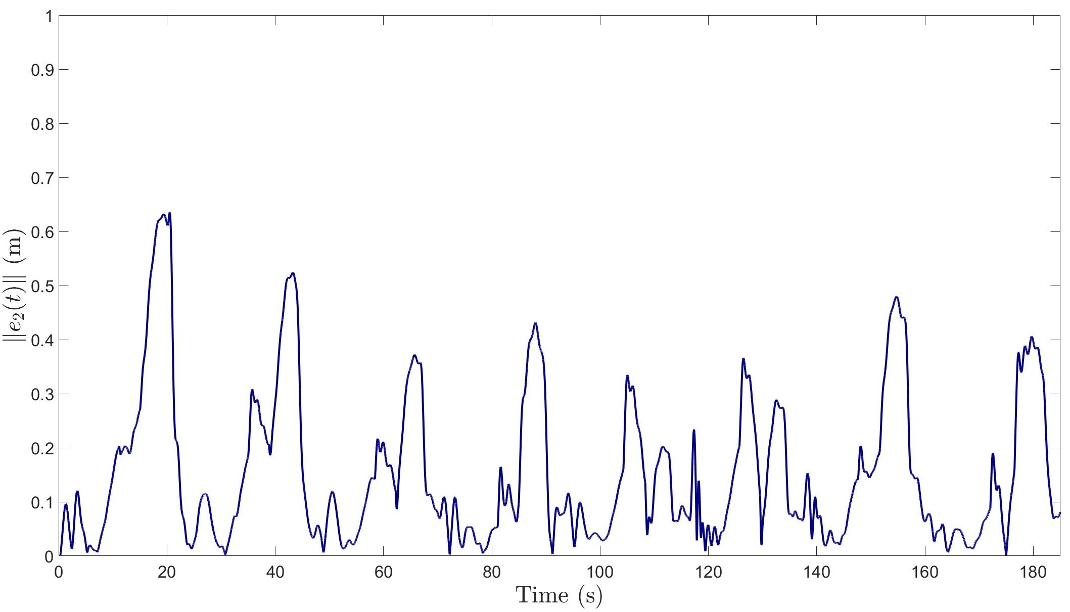
Figure 6: Estimation error $\|e_{2}(t)\|$. As indicated by the analysis, the estimation error converges when $x(t)\in\mathcal{F}$ and diverges when $x(t)\in\mathcal{F}^{c}$.

Figure 7: Evolution of $\|z(t)\|$. The dash-dot (vertical) lines indicate the switching interface of minimum and maximum dwell times, and the dashed (horizontal) lines indicate the prescribed upper bound and lower threshold.

Figure 8: Actual tracking error $\|e(t)\|$. The dash-dot lines indicate the switching interface of minimum and maximum dwell times.

Figure 9: Evolution of $V_{\sigma}(t)$. The dotted (vertical) lines indicate the time instants when the quadcopter crossed the feedback region boundary. The dashed (horizontal) lines indicate the prescribed $V_{M}$ and $V_{T}$ for $V_{\sigma}$.

IX Conclusion

A novel method that utilizes a switched systems approach to ensure path following stability under intermittent state feedback is presented. The presented method relieves the requirement of state feedback at all times. State estimates are used in the tracking control to compensate for the intermittence of state feedback. A Lyapunov-based, switched systems analysis is used to develop maximum and minimum dwell time conditions to guarantee stability of the overall system. The dwell time conditions allow the desired path to be completely outside of the feedback region, and a switching trajectory is designed to bring the states back into the feedback region before the error growth exceeds a defined threshold. The candidate switching trajectory switches between the desired path and the feedback region using smootherstep transition functions. A simulation and an experiment were performed to illustrate the robustness of the control and trajectory design. Future research will focus on development of an approximate optimal control approach using adaptive dynamic programming concepts to yield approximately optimal results. Further efforts will also examine cases where the feedback region is time-varying or unknown.

When using single integrator dynamics, $\dot{x}(t)=u+d(t)$, the resulting estimation error dynamics for the unstable subsystem is $\|\dot{e}_{2}(t)\|\leq\bar{d}$ , and the corresponding Lyapunov-like function derivative is $\dot{V}_{\sigma}(t)\leq\bar{d}\|e_{2}(t)\|$. By solving the ordinary differential equation for $\dot{e}_{2}(t)$, the estimation error $e_{2}(t)$ exhibits a linear growth that can be bounded as $e_{2}(t)\leq e_{2}(t_{i}^{u})+\bar{d}(t-t_{i}^{u})$. After substituting in the linear bound on $e_{2}(t)$, it follows that $\dot{V}_{\sigma}(t)\leq\bar{d}\|e_{2}(t_{i}^{u})\|+\bar{d}^{2}(t-t_{i}^{u})$, and solving the ordinary differential equation yields $V_{\sigma}(t)\leq\frac{1}{2}\bar{d}^{2}\left(t-t_{i}^{u}\right){}^{2}+\bar{d}\|e_{2}(t_{i}^{u})\|\left(t-t_{i}^{u}\right)+V_{\sigma}(z(t_{i}^{u}))$. After imposing $V_{\sigma}(t)\leq V_{M}$ as the upper bound constraint, the maximum dwell time can be derived by solving the quadratic equation and taking the positive root as

$$\Delta t_{i}^{u}\leq\frac{\left(\sqrt{\|e_{2}(t_{i}^{u})\|^{2}-2\left(V_{\sigma}(z(t_{i}^{u}))-V_{M}\right)}-\|e_{2}(t_{i}^{u})\|\right)}{\bar{d}}.$$

References

- [1] N. Gans, S. Hutchinson, and P. Corke, “Performance tests for visual servo control systems, with application to partitioned approaches to visual servo control,” Int. J. Rob. Res., vol. 22, no. 10, pp. 955–981, 2003.
- [2] S. Hutchinson, G. Hager, and P. Corke, “A tutorial on visual servo control,” IEEE Trans. Robot. Autom., vol. 12, no. 5, pp. 651–670, Oct. 1996.
- [3] N. Gans, G. Hu, K. Nagarajan, and W. E. Dixon, “Keeping multiple moving targets in the field of view of a mobile camera,” IEEE Trans. Robot. Autom., vol. 27, no. 4, pp. 822–828, 2011.
- [4] N. Gans, G. Hu, J. Shen, Y. Zhang, and W. E. Dixon, “Adaptive visual servo control to simultaneously stabilize image and pose error,” Mechatron., vol. 22, no. 4, pp. 410–422, 2012.
- [5] G. Hu, N. Gans, and W. E. Dixon, “Quaternion-based visual servo control in the presence of camera calibration error,” Int. J. Robust Nonlinear Control, vol. 20, no. 5, pp. 489–503, 2010.
- [6] G. Hu, N. Gans, N. Fitz-Coy, and W. E. Dixon, “Adaptive homography-based visual servo tracking control via a quaternion formulation,” IEEE Trans. Control Syst. Technol., vol. 18, no. 1, pp. 128–135, 2010.
- [7] G. Hu, W. Mackunis, N. Gans, W. E. Dixon, J. Chen, A. Behal, and D. Dawson, “Homography-based visual servo control with imperfect camera calibration,” IEEE Trans. Autom. Control, vol. 54, no. 6, pp. 1318–1324, 2009.
- [8] J. Chen, D. M. Dawson, W. E. Dixon, , and V. Chitrakaran, “Navigation function based visual servo control,” Automatica, vol. 43, pp. 1165–1177, 2007.
- [9] J. Chen, D. M. Dawson, W. E. Dixon, and A. Behal, “Adaptive homography-based visual servo tracking for fixed and camera-in-hand configurations,” IEEE Trans. Control Syst. Technol., vol. 13, pp. 814–825, 2005.
- [10] G. Palmieri, M. Palpacelli, M. Battistelli, and M. Callegari, “A comparison between position-based and image-based dynamic visual servoings in the control of a translating parallel manipulator,” J. Robot., vol. 2012, 2012.
- [11] N. Gans and S. Hutchinson, “Stable visual servoing through hybrid switched-system control,” IEEE Trans. Robot., vol. 23, no. 3, pp. 530–540, 2007.
- [12] G. Chesi and A. Vicino, “Visual servoing for large camera displacements,” IEEE Trans. Robot. Autom., vol. 20, no. 4, pp. 724–735, 2004.
- [13] N. R. Gans and S. A. Hutchinson, “A stable vision-based control scheme for nonholonomic vehicles to keep a landmark in the field of view,” in Proc. IEEE Int. Conf. Robot. Autom., Roma, Italy, Apr. 2007, pp. 2196–2201.
- [14] G. L. Mariottini, G. Oriolo, and D. Prattichizzo, “Image-based visual servoing for nonholonomic mobile robots using epipolar geometry,” IEEE Trans. Robot., vol. 23, no. 1, pp. 87–100, Feb. 2007.
- [15] G. Lopez-Nicolas, N. R. Gans, S. Bhattacharya, C. Sagues, J. J. Guerrero, and S. Hutchinson, “Homography-based control scheme for mobile robots with nonholonomic and field-of-view constraints,” IEEE Trans. Syst. Man Cybern., vol. 40, no. 4, pp. 1115–1127, Aug. 2010.
- [16] S. S. Mehta, G. Hu, A. P. Dani, and W. E. Dixon, “Multi-reference visual servo control of an unmanned ground vehicle,” in Proc. AIAA Guid. Navig. Control Conf., Honolulu, Hawaii, Aug. 2008.
- [17] B. Jia and S. Liu, “Switched visual servo control of nonholonomic mobile robots with field-of-view constraints based on homography,” Control Theory Technol., vol. 13, no. 4, pp. 311–320, 2015.
- [18] G. Klein and D. Murray, “Parallel tracking and mapping for small ar workspaces,” in IEEE ACM Int. Symp. Mixed Augment. Real., 2007, pp. 225–234.
- [19] A. J. Davison, I. D. Reid, N. D. Molton, and O. Stasse, “Monoslam: Real-time single camera slam,” IEEE Trans. Pattern Anal. Mach. Intell., vol. 29, no. 6, pp. 1052–1067, Jun. 2007.
- [20] D. Cremers, “Direct methods for 3d reconstruction and visual slam,” in IEEE IAPR Int. Conf. Mach. Vis. Appl., 2017, pp. 34–38.
- [21] B. Williams, M. Cummins, J. Neira, P. Newman, I. Reid, and J. Tardós, “A comparison of loop closing techniques in monocular slam,” Robot. Auton. Syst., vol. 57, no. 12, pp. 1188–1197, 2009.
- [22] C. Cadena, L. Carlone, H. Carrillo, Y. Latif, D. Scaramuzza, J. Neira, I. Reid, and J. Leonard, “Past, present, and future of simultaneous localization and mapping: Towards the robust-perception age,” IEEE Trans. Robot., vol. 32, no. 6, pp. 1309–1332, 2016.
- [23] E. Garcia and P. J. Antsaklis, “Adaptive stabilization of model-based networked control systems,” in Proc. Am. Control Conf., San Francisco, CA, USA, Jul. 2011, pp. 1094–1099.
- [24] S. S. Mehta, W. MacKunis, S. Subramanian, E. L. Pasiliao, and J. W. Curtis, “Stabilizing a nonlinear model-based networked control system with communication constraints,” in Proc. Am. Control Conf., Washington, DC, Jun. 2013, pp. 1570–1577.
- [25] E. Garcia and P. J. Antsaklis, “Model-based event-triggered control for systems with quantization and time-varying network delays,” IEEE Trans. Autom. Control, vol. 58, no. 2, pp. 422–434, Feb. 2013.
- [26] M. J. McCourt, E. Garcia, and P. J. Antsaklis, “Model-based event-triggered control of nonlinear dissipative systems,” in Proc. Am. Control Conf., Portland, Oregon, USA, Jun. 2014, pp. 5355–5360.
- [27] N. E. Leonard and A. Olshevsky, “Cooperative learning in multi-agent systems from intermittent measurements,” in Proc. IEEE Conf. Decis. Control, Florence, Italy, Dec. 2013, pp. 7492–7497.
- [28] J. Liang, Z. Wang, and X. Liu, “Distributed state estimation for discrete-time sensor networks with randomly varying nonlinearities and missing measurements,” IEEE Trans. Neural Netw., vol. 22, no. 3, pp. 486–496, Mar. 2011.
- [29] Y. Shi, H. Fang, and M. Yan, “Kalman filter-based adaptive control for networked systems with unknown parameters and randomly missing outputs,” Int. J. Robust Nonlinear Control, vol. 19, no. 18, pp. 1976–1992, Dec. 2009.
- [30] D. Liberzon, Switching in Systems and Control. Birkhauser, 2003.
- [31] G. Zhai, B. Hu, K. Yasuda, and A. N. Michel, “Stability analysis of switched systems with stable and unstable subsystems: An average dwell time approach,” Int. J. Syst. Sci., vol. 32, no. 8, pp. 1055–1061, Nov. 2001.
- [32] M. A. Müller and D. Liberzon, “Input/output-to-state stability and state-norm estimators for switched nonlinear systems,” Automatica, vol. 48, no. 9, pp. 2029–2039, 2012.
- [33] A. Parikh, T.-H. Cheng, H.-Y. Chen, and W. E. Dixon, “A switched systems framework for guaranteed convergence of image-based observers with intermittent measurements,” IEEE Trans. Robot., vol. 33, no. 2, pp. 266–280, April 2017.
- [34] H.-Y. Chen, Z. I. Bell, R. Licitra, and W. E. Dixon, “Switched systems approach to vision-based tracking control of wheeled mobile robots,” in Proc. IEEE Conf. Decis. Control, 2017, pp. 4902–4907.
- [35] A. Dani, N. Fischer, Z. Kan, and W. E. Dixon, “Globally exponentially stable observer for vision-based range estimation,” Mechatron., vol. 22, no. 4, pp. 381–389, Special Issue on Visual Servoing 2012.
- [36] Z. I. Bell, H.-Y. Chen, A. Parikh, and W. E. Dixon, “Single scene and path reconstruction with a monocular camera using integral concurrent learning,” in Proc. IEEE Conf. Decis. Control, 2017, pp. 3670–3675.
- [37] D. S. Ebert, Texturing & modeling: a procedural approach. Morgan Kaufmann, 2003.
- [38] “bebop_autonomy library,” http://bebop-autonomy.readthedocs.io.