Quantum features and signatures of quantum-thermal machines

Abstract

The aim of this book chapter is to indicate how quantum phenomena are affecting the operation of microscopic thermal machines, such as engines and refrigerators. As converting heat to work is one of the fundamental concerns in thermodynamics, the platform of quantum-thermal machines sheds light on thermodynamics in the quantum regime. This chapter focuses on the basic features of quantum mechanics, such as energy quantization, the uncertainty principle, quantum coherence and correlations, and their manifestation in microscopic thermal devices. In addition to indicating the peculiar behaviors of thermal-machines due to their non-classical features, we present quantum-thermodynamic signatures of these machines. Any violation of the classical bounds on thermodynamic measurements of these machines is a sufficient condition to conclude that quantum effects are present in the operation of that thermal machine. Experimental setups demonstrating some of the results are also presented.

I Introduction

Quantum mechanics is one of the greatest revolutions in the history of science. It changed the way we understand the world and demonstrates that the microscopic realm is governed by a theory that is fundamentally different from classical mechanics. Classical mechanics is formulated on the phase space and treats particles as points whereas quantum mechanics is described by wave functions and operators acting in Hilbert space. In the quantum framework, the classical perception of certainty is replaced by probability, and instead of being continuous, physical quantities are generally quantized. These significant differences result in peculiar phenomena that are observed only in the quantum regime.

Since the beginning, the development of quantum mechanics has been influenced by thermodynamics. Planck initiated the quantum era by introducing the quantization hypothesis to describe thermal radiation emitted from a black body; Einstein discovered stimulated emission while studying thermal equilibration between light and matter. In spite of the close historical relationship between quantum mechanics and thermodynamics, one could wonder if the quantum revolution would eventually shake the foundations of thermodynamics as it did with classical mechanics. Some of the early works in this direction studied the behavior of heat machines, which, besides their technological applications, were used to test the compliance with the laws of thermodynamics. Despite the effort focused on this direction, as of today, the fundamental laws and bounds of thermodynamics seem to hold also in the quantum regime.

Even though quantum mechanics complies with the laws of thermodynamics, classical and quantum heat machines still diverge from one another in a non trivial way. As we show in this chapter, not only are classical and quantum heat machines fundamentally different, but quantum mechanics allows the realization of classically inconceivable heat machines.

In order to identify the appearance and effects of quantum features in thermal machines, one should first have a clear notion of classical thermal machines. Throughout this chapter, we will use different notions or levels of classicality, starting from the purest definitions, (i.e., a system is classical only if it is precisely described by classical mechanics), and working toward less strict definitions, which consider systems governed by quantum Hamiltonians as classical as long as either their coherences or quantum correlations are zero. In this manner we obtain a thorough understanding of how different quantum features influence thermal devices.

The chapter is divided into three sections concerning three main quantum features and their corresponding thermodynamic signatures. In the first section, classicality will be considered as it is in classical thermodynamics, where the probability distribution is fully described by a phase space distribution without any constraint aside from normalization. In this section, quantum effects result only from the quantization of energy levels and the uncertainty principle, which sets some limitations on these probability distributions. These features alone lead to discrepancies in the behavior of classical and quantum heat machines.

The second section describes the effects of quantum coherence in thermal machines. Both the positive and negative implications of coherence are discussed. Furthermore, we present a recent experiment demonstrating some of these results. In these scenarios thermal machines that are governed by a quantum Hamiltonian, but can be fully described by their populations are considered classical (stochastic). In this context it’s also important to note that the preferred basis to describe thermal machine is the one in which measurements are preformed, typically, this will be the energy basis.

In the last section, we discuss the role of correlations in the operation of thermal machines. We demonstrate that quantum correlations can induce anomalous heat flow from a colder body to a hotter body, that can not be explained classically. Here, classicality refers to separable quantum states with zero discord, (i.e., only classical correlations are allowed). The chapter is structured so that each of the three main section is independent of the others.

II energy quantization and uncertainty principle

Classical and quantum mechanics provide different descriptions of the same physical system. This is true even for the simplest cases. As an example, consider a harmonic oscillator with mass $m$ and frequency $\omega$, in a thermal state at temperature $T$. Classically, its phase space distribution is given by the following Gaussian:

$$P_{HO}^{clas}(x,p)=\frac{\omega}{2\pi k_{B}T}e^{-\left(\frac{m\omega^{2}x^{2}}{2k_{B}T}+\frac{p^{2}}{2mk_{B}T}\right)}.$$ (1)

Strictly speaking, phase space distributions are not part of the quantum mechanics framework, as it is impossible to simultaneously determine the position and momentum of a system. Nevertheless, quasi-probability distributions, such as the Wigner function, share many properties with phase distributions Case (2008); Wigner (1932) and are considered the “closest quantum equivalent” to a phase space distribution. The Wigner function for the same harmonic oscillator at the same state is

$$P_{HO}^{quan}(x,p)=\frac{\tanh[\frac{\hbar\omega}{2k_{B}T}]}{\hbar\pi}e^{-\tanh[\frac{\hbar\omega}{2k_{B}T}]\left(\frac{m\omega x^{2}}{\hbar}+\frac{p^{2}}{\hbar m\omega}\right)}.$$ (2)

These two distributions coincide at the regime where the thermal energy is much larger than the quantization energy, i.e., $\frac{\hbar\omega}{k_{B}T}\ll 1.$ At this limit, the classical description is very precise, so quantum effects can be neglected. Nevertheless, the distributions diverge at low temperatures (see Fig. 1), where classical mechanics predicts a smaller and smaller position and momentum uncertainties, in contradiction with the uncertainty principle. In contrast, the Wigner distribution, Eq. (2), obeys the uncertainty principle at any temperature.

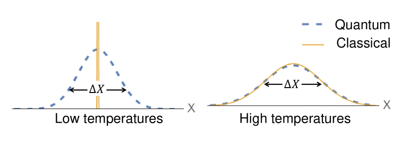
Figure 1: Position projection of the classical (yellow continuos line) and quantum (blue dashed line) phase space distributions for a harmonic oscillator in a thermal state. Both distributions coincide at high temperatures (right), but at low temperatures (left) the quantum Wigner distribution, in contrast with the classical one, has to comply with the uncertainty principle, forcing the distributions to diverge.

The differences between these distributions are based on the fact that quantum systems have to comply with the uncertainty principle Wigner (1932). Moreover, confining potentials impose boundary conditions that quantize the energy state, create a zero point energy, and establish a dependence of the system energy on the boundary conditions. The combination of all these effects results on different energy, heat capacity and other thermal properties Sundar et al. (2017) relatively to the ones predicted by classical mechanics and thermodynamics that neglect boundary effects Callen (1985). In this section of the chapter we will explore how those differences affect the performance of thermal heat machines. We will compare exactly the same heat machine, i.e., same working medium, same baths, same temperatures, etc., but in one case the behavior of the working medium is dictated by classical mechanics and in the other by quantum mechanics. In this section we do not consider the effects of quantum coherences or quantum correlations. These are left for subsequent sections of this chapter.

In particular, we consider an Otto heat machine Gelbwaser-Klimovsky et al. (2017); Quan et al. (2007a); Zheng and Poletti (2014) operating with a M-dimensional working medium, but a similar analysis can be done for other cycles. The Otto cycle is composed of the following four strokes (see Fig. 2): At point A of the cycle the working medium potential is $V_{h}(x_{1},...x_{M})\equiv V_{h}$. Its Hamiltonian is $H_{h}$ and its energy levels are $\{E_{n}^{h}\}$. The working medium is in thermal equilibrium with a hot bath at temperature $T_{h},$ so its state in the Hamiltonian energy basis is $\rho_{A}=Z_{T_{h}}^{-1}\sum_{n}e^{-\frac{E_{n}^{h}}{k_{B}T_{h}}}|n\rangle\langle n|,$ where $Z_{T_{h}}$ is the partition function. At $A$, the adiabatic stroke starts: the working medium is decoupled from the hot bath and the potential is slowly deformed until point B, where it reaches $V_{c}(x_{1},...x_{M})\equiv V_{c}$. Here, the Hamiltonian is $H_{c}$, and its energy levels are $\{E_{n}^{c}\}$. The deformation is slow enough for the process to fulfill the assumptions of the quantum adiabatic theorem Griffiths (2016), so the levels populations are the same $\rho_{B}=\rho_{A}$. At $B$, the system is coupled to the cold thermal bath at temperature $T_{c}$, initiating the cold isochoric stage. The system relaxes, achieving thermal equilibrium at C, i.e., $\rho_{C}=Z_{T_{c}}^{-1}\sum_{n}e^{-\frac{E_{n}^{c}}{k_{B}T_{c}}}|n\rangle\langle n|,$ where $Z_{T_{c}}$ is the partition function. Then, the working medium undergoes the second adiabatic stroke: it is decoupled from the bath and the potential is again slowly transformed back, reaching $V_{h}$ at $D$. Here too, we apply the quantum adiabatic theorem so $\rho_{D}=\rho_{C}.$ Finally, at this point, the second isochoric phase starts: the working medium is coupled again to the hot bath and equilibrates with it, returning to point A.

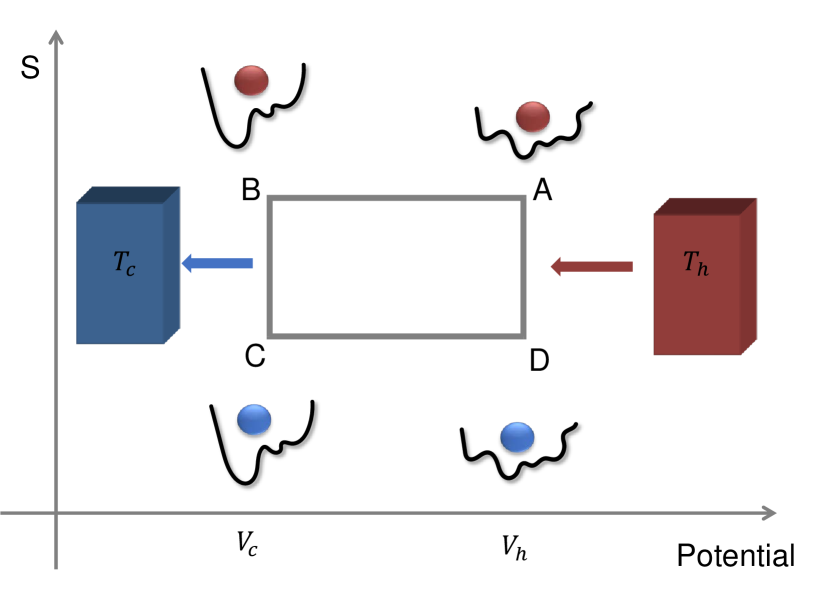
Figure 2: Otto cycle. The x-axis represents a parameter that controls the working medium potential and the y-axis represents its Von Neumann entropy.

One useful feature of the Otto cycle is that work and heat are exchanged during different parts of the cycle: work is transferred during the adiabatic processes and heat over the isochoric strokes. The heat flow from the hot bath is

$$Q_{h}=\langle H_{h}\rangle_{A}-\langle H_{h}\rangle_{D}=\sum_{n}E_{n}^{h}\left(\frac{e^{-\frac{E_{n}^{h}}{k_{B}T_{h}}}}{Z_{T_{h}}}-\frac{e^{-\frac{E_{n}^{c}}{k_{B}T_{c}}}}{Z_{T_{c}}}\right)$$ (3)

and from the cold bath is

$$Q_{c}=\langle H_{c}\rangle_{C}-\langle H_{c}\rangle_{B}=\sum_{n}E_{n}^{c}\left(\frac{e^{-\frac{E_{n}^{c}}{k_{B}T_{c}}}}{Z_{T_{c}}}-\frac{e^{-\frac{E_{n}^{h}}{k_{B}T_{h}}}}{Z_{T_{h}}}\right).$$ (4)

Using the first law of thermodynamics, the expression for the work can be obtained,

$$W=-Q_{h}-Q_{c}=\left(E_{n}^{c}-E_{n}^{h}\right)\left(\frac{e^{-\frac{E_{n}^{h}}{k_{B}T_{h}}}}{Z_{T_{h}}}-\frac{e^{-\frac{E_{n}^{c}}{k_{B}T_{c}}}}{Z_{T_{c}}}\right).$$ (5)

Here, we use the sign convention that energy flowing to the working medium is positive and flowing from the working medium is negative. The heat machine has several operating modes: for $W<0$ and $Q_{h}>0$, it is a heat engine and its thermal efficiency quantifies the amount of work extracted per unit of incoming heat, i.e., $\eta=\frac{-W}{Q_{h}}$; for $W>0$ and $Q_{c}>0$, it is a refrigerator and its efficiency or coefficient of performance measures how much energy flows from the cold bath per unit of invested work $COP=\frac{Q_{c}}{W}.$

For a classical Otto heat machine, whose working medium is an ideal gas, the operation mode is determined by the compression ratio $r=\frac{Vol_{c}}{Vol_{h}}$, ($Vol_{c}$ is the container volume at point C and $Vol_{h}$ is the container volume at point $A$): for $r>r_{Car}=\left(\frac{T_{h}}{T_{c}}\right)^{\frac{1}{\gamma-1}}$, it operates as a refrigerator and for $1<r<r_{Car}$ the classical Otto heat machine operates as an engine with an efficiency

$$\eta=1-\frac{1}{r^{\gamma-1}}\leq 1-\frac{1}{r_{Car}^{\gamma-1}}=\eta_{Car},$$ (6)

where $\eta_{Car}$ is the Carnot efficiency for an engine and $\gamma=\frac{C_{p}}{C_{v}}$ is the heat capacities ratio. An important property of the classical Otto machine is that, in order to extract work or extract heat from the cold bath, the working medium has to be compressible Callen (1985); Farris (1979); Mullen et al. (1975); Paolucci (2016); Gurtin et al. (2010). Otherwise, $r=1$ and $\eta=0$, precluding work extraction. This compression ratio is smaller than $r_{Car}$, hindering also the refrigerator operation. Here, quantum mechanics provides heat machines with an advantage over their classical counterparts. As it was shown on Gelbwaser-Klimovsky et al. (2017) and we explain below, once the working medium is governed by quantum laws instead of classical mechanics, compressibility is no longer required for work extraction or for cooling down the cold bath. Quantum mechanics allows the realization of heat machines with incompressible working media, opening the possibility for creating classically inconceivable heat machines.

One feature of a classical ideal gas undergoing an Otto cycle is that it is always at equilibrium, so at every point of the cycle it is possible to define the ideal gas temperature. This is not always true for a quantum working medium. For example, at $B,$ the working medium is at the state $\rho_{B}=Z_{T_{h}}^{-1}\sum_{n}e^{-\frac{E_{n}^{h}}{k_{B}T_{h}}}|n\rangle\langle n|,$ which is a Boltzmann distribution of the energy levels at point A ($\{E_{n}^{h}\}$) instead of point B ($\{E_{n}^{c}\}$). So, in general, the state $\rho_{B}$ is not a thermal equilibrium state with respect to the Hamiltonian at point B. The only exception is if the transformation homogeneously scales the energy levels i.e., $E_{n}^{c}=qE_{n}^{h}$, where $q$ is independent of $n$. Under this condition we can rewrite the state at B as $\rho_{B}=Z_{qT_{h}}^{-1}\sum_{n}e^{-\frac{E_{n}^{c}}{k_{B}qT_{h}}}|n\rangle\langle n|,$ which is a Boltzmann distribution at temperature $qT_{h}$ of the energy levels at point B. In a similar way, the state at D, $\rho_{D}=Z_{T_{c}}^{-1}\sum_{n}e^{-\frac{E_{n}^{c}}{k_{B}T_{c}}}|n\rangle\langle n|=Z_{T_{c}/q}^{-1}\sum_{n}e^{-\frac{qE_{n}^{h}}{k_{B}T_{c}}}|n\rangle\langle n|$ is a Boltzmann distribution at temperature $T_{c}/q$ of the energy levels at point D. Most of the research on quantum Otto cycles has focused on this type of transformations Quan et al. (2007a); Zheng and Poletti (2014) which includes the length change of a 1D infinite well Quan (2009), frequency shift of a 1D harmonic oscillator Kosloff and Rezek (2017) or any other scale invariant transformation Zheng and Poletti (2015). We will first study the differences between classical and quantum heat machines undergoing homogeneously energy scaling, which allows the working medium to be in a thermal state during the whole cycle. Then, we will explore the regime of inhomogeneous energy scaling, which has been seldom studied, with few exceptions Uzdin and Kosloff (2014); Quan et al. (2005). For an inhomogeneous energy scaling, the working medium deviates from a thermal state during the adiabatic strokes, resulting on more striking discrepancies between the operation of classical and quantum heat machines, and providing the later with more noteworthy advantages.

II.1 Homogeneous energy scaling: work and heat corrections

In the case of the homogeneous energy scaling, the working medium is in a thermal state during the whole cycle. So we can use Wigner’s original computation to calculate the quantum corrections to the performance of a heat machine. In 1932, Wigner calculated the quantum corrections to the quasiprobability distribution of a M-dimensional system in a potential $V$ at thermal equilibrium at temperature $T$ Wigner (1932). After integrating the momentum, the not normalized position distribution is given by a series expansion on $\hbar$:

$$\int...\int dp_{1}...dp_{M}P^{quan}(x_{1},...,x_{n};p_{1},...p_{M})=P^{clas}+\hbar^{2}P_{2}^{quan}+\hbar^{4}P_{4}^{quan}+O(\hbar^{6}),$$ (7)

where

$$P^{clas}=e^{-\frac{V}{k_{B}T}}$$ (8)

is the classical phase space distribution and $P_{2n}^{quan}$ are quantum corrections that depend on the potential and its derivatives but not on $\hbar$. For example, the first quantum correction is

$$P_{2}^{quan}=e^{-\frac{V}{k_{B}T}}\left[-\frac{1}{12\left(k_{B}T\right)^{2}}\sum_{k}\frac{1}{m_{k}}\frac{\partial^{2}V}{\partial x_{k}^{2}}+\frac{1}{24(k_{B}T)^{3}}\sum_{k}\frac{1}{m_{k}}\left(\frac{\partial V}{\partial x_{k}}\right)^{2}\right].$$ (9)

At high temperatures, the Wigner function tends to the classical phase space distribution, i.e., $\int...\int dp_{1}...dp_{M}P^{quan}(x_{1},...,x_{n};p_{1},...p_{M})\approx e^{-\frac{V}{k_{B}T}}$. But as the temperature decreases, quantum corrections need to be included to prevent the violation of the uncertainty principle. These corrections change the expectation value of the energy,

$$\langle H\rangle_{T}=E_{clas}(V,T)+\hbar^{2}E_{2,QC}(V,T)+O(\hbar^{4}),$$ (10)

where $E_{clas}(V,T)$ corresponds to the system energy predicted by classical mechanics and $E_{2,QC}(V,T)$ is the first quantum correction

$$E_{2,QC}(V,T)=$$

$$\frac{1}{\int P^{clas}}\left[\frac{1}{24k_{B}T}\int\sum\frac{1}{m_{k}}\frac{\partial^{2}V}{\partial^{2}x_{k}}P^{clas}+\int V\times P_{2}^{quan}-\frac{\int V\times P^{clas}\int P_{2}^{quan}}{\int P^{clas}}\right]$$ (11)

where all the integrals are over all the positions, $x_{1},...,x_{M}.$ The quantum corrections to the energy affect the output of a heat machine. For example, the heat exchanged with the hot bath, including quantum corrections of the order $\hbar^{2}$ is

$$Q_{h}=Q_{h}^{clas}+\hbar^{2}\left(E_{2,QC}(V_{h},T_{h})-E_{2,QC}(V_{h},T_{c}/q)\right)+O(\hbar^{4}),$$ (12)

where $Q_{h}^{clas}$ corresponds to the heat that a classical working medium would exchange with the hot bath during the Otto cycle, and the other terms are corrections that have to be included for a quantum working medium. In the same way, we can calculate the exchanged work,

$$W=W^{clas}-\hbar^{2}\left(E_{2,QC}(V_{h},T_{h})-E_{2,QC}(V_{h},T_{c}/q)+E_{2,QC}(V_{c},T_{c})-E_{2,QC}(V_{c},qT_{h})\right)+O(\hbar^{4}),$$ (13)

where $W^{clas}$ corresponds to the work exchange by a classical Otto engine and the rest are the quantum corrections. As we explain later (see Eq. (17)), in order to extract work, i.e., $W\text{<0, }$ the scaling factor of the energy levels has to comply with the following inequality: $\frac{T_{c}}{T_{h}}<q<1$.

For 1D systems in an Otto cycle with potentials $V_{c}=a_{c}x^{2n}$ and $V_{h}=a_{h}x^{2n}$, the scaling factor between energy levels is $q=\left(\frac{a_{c}}{a_{h}}\right)^{\frac{1}{1+n}}$ Zheng and Poletti (2014) and the correction of order $\hbar^{2}$ to the exchanged work can be analytically calculated. It is equal to

$$-\frac{\hbar^{2}\pi(2n^{2}+n-1)\csc[\frac{\pi}{2n}]}{12m(\Gamma[\frac{1}{2n}])^{2}}\left(\frac{a_{c}}{k_{B}T_{c}}\right)^{\frac{1}{n}}\left(1-\frac{1}{q}\right)\left(1-\left(\frac{T_{c}}{qT_{h}}\right)^{\frac{1}{n}}\right),$$ (14)

where $\Gamma$ is the gamma function. The correction can be positive or negative, but in the regime of work extraction, $W<0$, it is always positive, i.e., it always reduces the work extraction.

The first quantum correction starts being relevant when the operation temperatures are not so high and any of the Wigner functions during the cycle deviate from the classical phase space distribution. As temperatures decrease even more, higher order corrections should be considered. At least for 1D systems, there are recursive formulas that could be used to calculate any $P_{2n}^{quan}$ Coffey et al. (2007), from which the full quantum corrections to the work and heat could be calculated. Nevertheless, this is not a practical approach and we will now introduce a simpler strategy that is exact at any temperature.

Using the fact that the energy levels are homogeneously scaled, $E_{n}^{c}=qE_{n}^{h}$, the expressions for the exchanged heat and work, Eqs. (3)-(5), can be rewritten. Consider for example $Q_{h}$ (Eq. (3)). Using the relation between the energy levels this equation becomes

$$Q_{h}=\sum_{n}E_{n}^{h}\left(\frac{e^{-\frac{E_{n}^{h}}{k_{B}T_{h}}}}{Z_{T_{h}}}-\frac{e^{-\frac{qE_{n}^{h}}{k_{B}T_{c}}}}{Z_{T_{c}/q}}\right)=$$

$$\int_{T_{c}/q}^{T_{h}}\frac{d}{dT}\left(\sum_{n}E_{n}^{h}\frac{e^{-\frac{E_{n}^{h}}{k_{B}T}}}{Z_{T}}\right)dT=\int_{T_{c}/q}^{T_{h}}\frac{d\langle H_{h}\rangle_{T}}{dT}dT=\int_{T_{c}/q}^{T_{h}}C_{v}dT,$$ (15)

where we have used the fundamental theorem of calculus and $C_{v}$ is the heat capacity of a thermal state at temperature $T$ with Hamiltonian $H_{h}$. In the same way, we can rewrite the equations for $Q_{c}$ and $W$ as:

$$Q_{c}=-q\int_{T_{c}/q}^{T_{h}}C_{v}dT;$$ (16)

$$W=(q-1)\int_{T_{c}/q}^{T_{h}}C_{v}dT;$$ (17)

Because the heat capacity is always positive, work is extracted only if $\frac{T_{c}}{T_{h}}<q<1$. We leave the readers to prove this as an exercise. All the information about the nature of the working medium is contained only on the heat capacity, $C_{v}.$ If the working medium is a classical system, classical mechanics should be used to compute $C_{v}$. If the working medium is a quantum system, quantum mechanics should be used to calculate $C_{v}.$ Consider for example a working medium composed of $N$ independent harmonic oscillators at thermal equilibrium at temperature $T$. A classical description, based on the equipartition theorem, assigns a contribution of $\frac{k_{B}}{2}$ for each quadratic degree of freedom of the Hamiltonian. There are two quadratic degrees of freedom for each harmonic oscillator, x and p. Therefore, classically $C_{v}^{HO,clas}=Nk_{B}$ at any $T.$ In contrast, if we use quantum mechanics for calculating the heat capacity, we will get $C_{v}^{HO,quan}=Nk_{B}\left(\frac{\hbar\omega}{2k_{B}T}csch\left[\frac{\hbar\omega}{2k_{B}T}\right]\right)^{2},$ which is temperature dependent (see Fig. 3-left). Because, $C_{v}^{HO,quan}\leq C_{v}^{HO,clas},$ the heat and work exchanged by a heat machine made of a quantum harmonic oscillator working medium is always less than its classical counterpart, turning the classical heat machine into a better election if we want to increase the heat or work exchange.

Nevertheless, the advantage of the classical heat machine is not a general feature and depends on the type of working medium, which is determined by the potentials, and the temperature range. As an example consider a working medium composed of particles of mass $m$ in a one dimensional box of length $L$. The quantum heat capacity is larger than its classical counterpart at not so low temperatures, i.e., $k_{B}T\gtrsim\frac{\hbar^{2}\pi^{2}}{2mL^{2}}$ (see Fig. 3-right). Thus, for a one dimensional box potential, a quantum heat machine may have a larger output than its classical counterpart, i.e., extracts more work and exchanges more heat with the thermal baths. What are the required features for a potential in order to boost the heat machine output and how they relate with other quantum effects, such as the Wigner function negativity, are still open questions that should be further investigated.

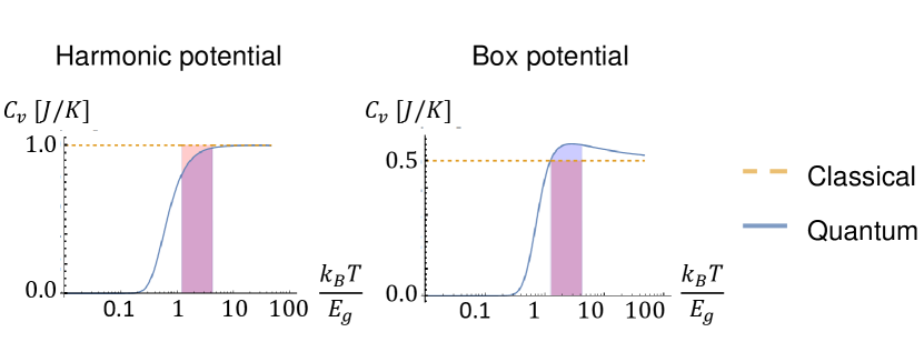
Figure 3: Classical (yellow dashed line) and quantum (blue continuous line) heat capacities as function of the temperature normalized by the working medium ground state energy. The area below the curves, enclosed by the temperatures $T_{c}/q$ and $T_{h},$ is proportional to the work and heat exchange by a classical or a quantum heat machine. For 1D harmonic oscillator potentials (left), the classical heat machine has a larger output than its quantum counterpart (see red area above the quantum curve). In contrast, for a particle in a 1D box (right), the output of the quantum heat machine is larger (see blue area above the classical curve).

Up to this point we have talked about the work and heat exchange. But what about the thermal efficiencies, such as the engine efficiency or the coefficient of performance of a refrigerator? Because these quantities are rates of the exchanged work and the heat from one of the baths,

$$\eta=-\frac{W}{Q_{h}}=1-q;\quad COP=\frac{Q_{c}}{W}=\frac{q}{1-q},$$ (18)

they do not depend on the heat capacity, and therefore they do not depend on the quantum or classical nature of the working medium. Thus, $\eta^{quan}=\eta^{clas}$ and $COP^{quan}=COP^{clas}.$ The efficiencies only depend on the potential deformation, which is characterized by the energy levels scaling factor, $q$.

II.2 Inhomogeneous energy scaling and the efficiency divergence

Could the efficiency of a quantum heat machine be greater than or at least different from its classical counterpart? Do quantum heat machines have any fundamental advantage over their classical counterparts? The answer to both questions is yes, but the potential transformation should be such that the energy levels are not homogeneously scaled, i.e., $E_{n}^{c}\neq qE_{n}^{h}.$ As we show below, not only the performance is different, but energy quantization enables the realization of classically inconceivable heat machines, such as those operating with an incompressible working medium Gelbwaser-Klimovsky et al. (2017).

We exemplify these effects in a particular 2D example, but a similar analysis can be done for higher dimensions, such as 3D, or other potentials Gelbwaser-Klimovsky et al. (2017). Here, we consider a working medium contained in a two dimensional box. At points D and A of the cycle, the measurements of the box are $L_{x}^{h}$ and $L_{y}^{h}$. At points B and C, they are $L_{x}^{c}$ and $L_{y}^{c}$ . If the working medium is incompressible, the box transformations during the adiabatic strokes have to keep the area constant: if the length along $x$ is increased by a factor $j$, $L_{x}^{c}=jL_{x}^{h},$ then the size along $y$ has to be scaled by a factor $\frac{1}{j}$, $L_{y}^{c}=\frac{1}{j}L_{y}^{h}$. These transformations correspond to the red lines on the plots on Fig. 4.

During the adiabatic strokes, the adiabatic invariants have to be constant. The adiabatic invariant for a classical particle of mass $m$ and energy $E$ in a two dimensional box of area A is Brown et al. (1987)

$$\mu=2\pi mEA,$$ (19)

which implies that during the adiabatic transformation $mEA$ is constant. So, for a constant area adiabatic transformation, the energy of the classical working medium does not change, precluding the work extraction. This is true for any classical non-interacting system, from an ideal gas to a single particle. Furthermore, the lack of work extraction is confirmed by taking the classical limit ($\hbar\rightarrow 0$) of the quantum calculation for the work, (see Eq. (5) and Fig. 4-center).

For a quantum working medium, one has to consider the energy levels, which are given by

$$E_{n_{x},n_{y}}^{i}=\frac{\hbar^{2}\pi^{2}}{2m}\left(\left(\frac{n_{x}}{L_{x}^{i}}\right)^{2}+\left(\frac{n_{y}}{L_{y}^{i}}\right)^{2}\right),$$ (20)

where $n_{x}$ and $n_{y}$ are integers, and $i=\{h,c\}$. For the constant area transformations, as long as $j\neq 1,$ the energy levels scaling is inhomogeneous and the classical and quantum efficiencies diverge. Moreover, Eq. (19) is not an adiabatic invariant at the quantum regime, where constant level populations is enough to warrant adiabaticity. As stated by the quantum adiabatic theorem, adiabaticity is achieved by performing the transformation slowly enough. This can be realized for constant area deformations that change the energy of the working medium. For simplicity, here we are assuming that the quantum working medium is composed of distinguishable particles.

In contrast to the classical heat machine, a quantum heat machine can be highly efficient, i.e., operate close to the Carnot limit, even for constant area transformations (see red line on Fig. 4-center). This opens the possibility of creating heat machines using incompressible working media, which classically would be impossible. Despite the increase in efficiency, quantum heat machines are always limited by the Carnot bound and fully comply with the second law of thermodynamics.

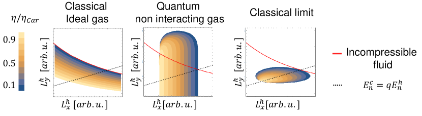
Figure 4: Heat engine efficiency for a 2D potential box normalized by the Carnot efficiency. At point B and C of the cycle, the box lengths are such that $L_{y}^{c}/L_{x}^{c}=0.25$ and the temperature ratio is $T_{h}/T_{c}=2$. The plots show the results for different values of the box lengths at points D and A of the cycle, i.e., $L_{x}^{h}$ and $L_{y}^{h}$. An incompressible working medium can only undergo area preserving transformations, here indicated by the red line. For these transformations there is no work extraction for a classical working medium, independently if it is an ideal gas (left) or the classical limit $\hbar\rightarrow 0$ (right) of a quantum particle in a box. In contrast, a quantum working medium (center) can be highly efficient, $\eta/\eta_{Car}>0.9$, even for area preserving transformations. The dashed black line indicates transformations where the energy levels are homogeneously scaled and the quantum and classical efficiency coincide.

The quantum model of a particle in a two dimensional box is not the exact counterpart of a classical ideal gas heat machine. For an ideal gas, changes on one of the directions affect the other, redistributing the energy. In contrast, our quantum model is composed of two independent degrees of freedom that do not interact between themselves. Its classical limit, $\hbar\rightarrow 0$, corresponds to a different performance than the ideal gas heat machine (see Fig. 4 right and left, respectively). In any case, for a classical working medium contained in a two dimensional box, either an ideal gas or one composed of two independent degrees of freedom, classical adiabatic invariants forbid the work extraction for constant area transformations. This differs from the quantum case where quantum adiabatic invariants still allow work extraction. Further extension of this work should confirm if, for constant area transformations, work can be extracted using a “quantum ideal gas” . The gas Hamiltonian should include non-trivial interactions among its degrees of freedom, i.e., non-linear couplings, in order to avoid the formation of normal modes and to achieve full thermalization. Further works should also consider the effects of different quantum statistics, such as Fermi-Dirac or Bose-Einstein statistics.

In summary, in this section we have analyzed the differences between heat machines with a working medium governed either by classical or quantum mechanics. The difference in their operation is determined by the type of Hamiltonian transformation: if the energy levels are homogeneously scaled, the work and heat exchange may diverge, but the efficiencies are the same. In contrast, for inhomogeneous energy level scaling, the efficiencies also diverge, allowing the extraction of work with incompressible working fluids and opening for the realization of classically impossible heat machines. Future research should focus on finding other fundamental differences between the operation of classical and quantum heat machines. In this section, we have not studied quantum coherences or correlations. All the quantum effects that have been considered are the basic quantum effects of a confined system: energy quantization and the uncertainty principle. Nevertheless, as we showed, this is enough for heat machines to have fundamentally different performances.

III Coherence and small action regime

Quantum coherence is one of the underlying principles of quantum mechanics that allows us to distinguish between classical and quantum phenomena. Historically, quantum coherence clarified the basic aspect of wave-particle duality in physical objects. Nowadays, scientists are trying to reveal the role of quantum coherence in biological, chemical, and physical systems and learn how to exploit it as a resource Streltsov et al. (2017); Gelbwaser-Klimovsky and Aspuru-Guzik (2017).

In recent years, the role of coherence in quantum thermodynamics has been studied extensively. One fundamental question is how, if at all, quantum coherence can be extracted as thermodynamic work Lostaglio et al. (2015); Korzekwa et al. (2016); Skrzypczyk et al. (2013); Åberg (2014); Horodecki and Oppenheim (2013); Niedenzu et al. (2015); Gelbwaser-Klimovsky and Kurizki (2015). The role of coherence in the operation of quantum thermal machines is another area of investigation. For example, it has been shown that noise-induced coherence can break detailed balance and enable the removel of additional power from a laser or a photocell heat engine Scully et al. (2011). It has also been shown that coherence enhances heat flow between a quantum engine and the thermal bath, impling that coherence plays an important role in the operation of quantum refrigerators Rahav et al. (2012); Mitchison et al. (2015); Latune et al. (2018). Engines subject to coherent and squeezed thermal baths have also been studied Roßnagel et al. (2014); Manzano et al. (2016); Alicki and Gelbwaser-Klimovsky (2015). While such engines can exceed the Carnot efficiency or even extract work from a single bath M. O. Scully, M. S. Zubairy, G. S. Agarwal, H. Walther (2003); Gelbwaser-Klimovsky et al. (2013a), they do not break the second-law of thermodynamics as useful work is hidden in the bath Niedenzu et al. (2016). In this context, it is important to note, that the Carnot bound is a relevant reference point only when thermal bath are considered.

However, the existence of coherence in quantum thermal machines is not always beneficial for their operation. In Brandner et al. (2017) it was shown that for slow driving in the linear response of a Stirling-type engine coherence leads to power loss. This detraction in the performance of the engine is related to the phenomenon of quantum friction Feldmann and Kosloff (2000); Kosloff and Feldmann (2002); Plastina et al. (2014); Alecce et al. (2015). In this section we will discuss both positive and negative implications of coherence. In particular, we will present a study by Uzdin et al. Uzdin et al. (2015, 2016) that reveals the thermodynamic equivalence of different types of engines in the small action regime. In this regime it has further been shown that coherence enhances power extraction. We further present a recent experiment Klatzow et al. (2017) that demonstrate these two findings. At the end of this section we will discuss the origin of quantum friction which degrades the performance of thermal machines.

III.1 Heat machines types and the mathematical description

III.1.1 Heat machine types

In this section, we will consider the three most common types of heat engines: the continuous engine, the two-stroke engine, and the four-stroke engine (see Fig. 5). The elementary components for assembling a quantum heat engine are two heat baths at different temperatures, $T_{h}$ and $T_{c}$, where the subscripts $h(c)$ correspond to hot(cold), such that $T_{h}>T_{c}$, a work source, which is used for consuming/extracting energy in/out of the engine, and as the working medium, a quantum system, that couples the different components of the engine.

As was discussed in the previous chapters and in Refs. Kosloff and Levy (2014); Chen et al. (2017); Geva and Kosloff (1992); Correa (2014); Esposito et al. (2010), the working medium can be described by different types of quantum systems. Here, we treat the working medium as a three-level system. The three-level setup was first studied by Scovil and DuBois Scovil and Schulz-DuBois (1959) and is considered the pioneering work in the field. This model was later studied by Kosloff et al. Kosloff and Levy (2014); Geva and Kosloff (1994); Palao et al. (2001) who employed a quantum dynamical description, which reveals the significance of quantum effects in the study of thermodynamics of microscopic heat engines. Besides being an elementary model, the three-level engine has demonstrated quantum signatures in nitrogen-vacancy centers experimental setup Klatzow et al. (2017). This will be discussed in more detail in section III.4. In Fig. 5 the three types of quantum heat engines that are compromised of three-level systems are described schematically. The Hamiltonian of the system, including the driving Hamiltonian, takes the form $H(t)=H_{o}+H_{w}(t)$ with

$$H_{o} = \hbar\omega\left|2\right>\left<2\right|+\hbar\omega_{h}\left|3\right>\left<3\right|$$ (21)

$$H_{w} = \epsilon(t)\exp(i\omega t)\left|1\right>\left<2\right|+\text{H.c.}.$$

Here, $H_{o}$ is the bare Hamiltonian, where the energy of level one is assumed to be zero. The system is periodically driven with the frequency $\omega=\omega_{h}-\omega_{c}$ which is in resonance with the transition frequency between the first and second levels. The driving Hamiltonian, $H_{w}(t)$, is expressed after performing the rotating wave approximation (assuming $\epsilon\ll\omega$), and H.c. stands for the Hermitian conjugate. The interaction with the bath will be described explicitly below for both the Markovian and non-Markovian regimes.

Continuous engines- are machines in which all components of the engine are simultaneously coupled through the working medium Levy and Kosloff (2012); Kosloff and Levy (2014); Gelbwaser-Klimovsky et al. (2013b, 2015), attaining a steady-state operation. The hot bath couples the first and third levels while the cold bath couples the second and third levels. The coupling to the heat baths generates a population inversion between the first and second levels, which is used to extract work by amplifying a driving field connecting the two levels. In the weak driving limit, the condition for population inversion can be simplified to $\frac{T_{h}}{T_{c}}>\frac{\omega_{h}}{\omega_{c}}>1$. The device can operate as a refrigerator by simply changing the direction of the inequality $\frac{T_{h}}{T_{c}}<\frac{\omega_{h}}{\omega_{c}}$ Levy et al. (2012). We remark that population inversion is not the only mechanism to gain power from a quantum heat engine. In Ref. Harris (2016) electromagnetically induced transparency mechanism was suggested to obtain bright narrow emission light without population inversion, and this was later demonstrated experimentally Zou et al. (2017) with cold Rb atoms.

Two-stroke engines- operate in a two stage mode A. E. Allahverdyan, R.S. Johal and G. Mahler (2008); Quan et al. (2007b). In the first stroke, the quantum system is coupled to both the cold and hot baths, whereas in the second stroke, after the system is decoupled from the heat baths, work is extracted from the quantum system via a coupling to an external field. In the example of the three level system, at the end of the first stroke population inversion between the first and second levels is created, and in the second stroke this population inversion is exploited to extract useful work from the engine (see Fig. 5).

Four-stroke engines- are perhaps the most familiar types of engines, as they include the Otto and Carnot engines. The Otto cycle, which was already introduced in Sec. II is comprised of four strokes, two isochores and two adiabats Feldmann and Kosloff (2000); Kosloff and Rezek (2017); Zhang et al. (2014). In Fig. 5, we describe the quantum analog of the four-stroke Otto engine. In the first stroke, levels one and three are coupled to the hot bath, and heat flows into the working medium. In the second stroke, work is invested without any transfer of heat, and in the third stroke levels three and two are coupled to the cold bath, and heat flows out of the working medium. In the last stroke, the working medium is again decoupled from the heat bath and work is extracted from the engine, completing a full cycle.

The stroke-type engines operate repeatedly, and each cycle takes a certain amount of time $\tau_{cyc}$. Defining where the cycle begins is arbitrary, as long as all four stroke are completed. Unlike the continuous engines, the stroke-type engines do not reach a steady state operation, but rather, they reach a limit cycle, where at the end of each cycle the state of the quantum system is the same. The efficiencies for all of the engines described in Fig. 5 are given by $\eta_{otto}=1-\frac{\omega_{c}}{\omega_{h}}$, which is termed the quantum otto efficiency Feldmann and Kosloff (2000); Kosloff and Rezek (2017); Kosloff and Levy (2014). We leave the readers to prove this as an exercise. For simplicity, the description of the stroke-engines above is based solely on population inversion and does not require description of quantum coherence. In this sense, these engines describe a stochastic (classical) operation of the engines. In the following sections we will see that the presence of quantum coherence will have an influence on the thermodynamics of these thermal devices.

The mathematical description of these engines requires tools from the theory of open quantum systems. While the work strokes are described using a unitary propagator $U$ which preserve the entropy of the quantum system, the coupling to the bath introduces irreversible dynamics accompanied with entropy generation. The dynamics of the engine is described by a completely-positive and trace-preserving map. In the Markovian regime this can be achieved using the Lindblad-Gorini-Kossakowski-Sudarshan (LGKS) master equation Lindblad (1976); V. Gorini, A. Kossakowski and E.C.G. Sudarshan (1976), which is described in detail in the next section. Extending the study of quantum heat machines beyond the Markovian regime and the weak system-bath coupling limit can be preformed using Green’s functions Esposito et al. (2015), the polaron transformation Gelbwaser-Klimovsky and Aspuru-Guzik (2015); Segal (2014); Xu et al. (2016), or using simulations based on the stochastic surrogate Hamiltonian Gil Katz, David Gelman, Mark A. Ratner, and Ronnie Kosloff (2008). Here, we will take a different approach based on the idea of heat exchangers Uzdin et al. (2016), which will be described in detail in Sec. III.1.3.

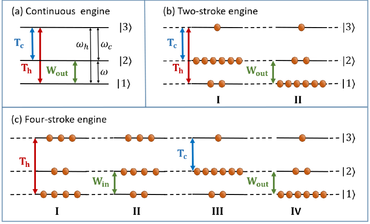
Figure 5: Scheme of three different types of heat engines: (a) a continuous engine, (b) a two-stroke engine, and (c) a four-stroke engine.

III.1.2 Markovian regime and Liouville space

In the Markovian regime, the dynamics of the system (the working medium) is described by a reduced description for the density operator $\rho$ and takes the form of the LGKS Markovian master equation H.-P. Breuer and F. Petruccione (2002); Lindblad (1976); V. Gorini, A. Kossakowski and E.C.G. Sudarshan (1976):

$$i\hbar\frac{d}{dt}\rho=L(\rho)\equiv[H_{s},\rho]+i\sum_{k}S_{k}\rho S_{k}^{\dagger}-\frac{1}{2}S_{k}^{\dagger}S_{k}\rho-\frac{1}{2}\rho S_{k}^{\dagger}S_{k}.$$ (22)

The $S_{k}$ operators depend on the system-bath coupling and on the properties of the bath, including the temperature and the correlations H.-P. Breuer and F. Petruccione (2002). In following, we concentrate on thermal generators $L$ that asymptotically induce the system to evolve into a Gibbs state, $\rho_{th}=\exp(-\beta H_{s})/Z$, with the inverse bath temperature $\beta=1/k_{B}T$ and the partition function $Z$. This type of generator can be derived from a microscopic Hamiltonian dicription in the weak system-bath coupling limit Davies (1974); H.-P. Breuer and F. Petruccione (2002) and for a collision model in the low density limit Dumcke (1985). The necessity of a microscopic derivation was discussed in Levy and Kosloff (2014), where it was shown that a local phenomenological description may lead to a violation of the second law of thermodynamics.

To derive the results of this chapter, we analyze the dynamics in the extended Liouville space. In this space, any matrix representation of an operator acting in a Hilbert space is mapped to a vector. That is, for a general matrix $B$ acting in Hilbert space: $B_{N\times N}\rightarrow\left|B\right>_{1\times N^{2}}$. Given this index mapping, the master equation (22) in Liouville space reads:

$$i\hbar\frac{d}{dt}\left|\rho\right>\equiv\mathcal{L}\left|\rho\right>\equiv(\mathcal{H}_{s}+\mathcal{L}^{d})\left|\rho\right>.$$ (23)

The super-operator $\mathcal{H}_{s}$ is represented by a Hermitian $N^{2}\times N^{2}$ matrix that corresponds to the first term on the right hand side of (22), and the super-operator $\mathcal{L}^{d}$ is a non-Hermitian $N^{2}\times N^{2}$ matrix that corresponds to the dissipative terms in (22). In this chapter, we use calligraphic letters to describe super-operators acting in Liouville space and ordinary letters for operators acting on a Hilbert space. We also chose a specific map known as the “vec-ing”. More details on the Liouville-space representation of quantum mechanics are presented in Box 1.

The LGKS operators in Hilbert space that describes the coupling of the system to the hot bath are expressed as

$$S_{1}^{h} = \sqrt{\gamma_{h}}e^{-\hbar\omega_{h}\beta_{h}}\left|3\right>\left<1\right|,$$ (24)

$$S_{2}^{h} = \sqrt{\gamma_{h}}\left|1\right>\left<3\right|,$$

and those to the cold bath as

$$S_{1}^{c} = \sqrt{\gamma_{c}}e^{-\hbar\omega_{c}\beta_{c}}\left|3\right>\left<2\right|,$$ (25)

$$S_{2}^{c} = \sqrt{\gamma_{c}}\left|2\right>\left<3\right|.$$

These operators form the dissipators $\mathcal{L}_{h}$ and $\mathcal{L}_{c}$ respectively. In the weak coupling limit, the parameters $\gamma_{h}$ and $\gamma_{c}$ are given by the Fourier-transforms of the baths correlation functions H.-P. Breuer and F. Petruccione (2002). Without any external driving, the coupling to the baths will lead asymptotically to a Boltzmann factor ratio of the populations, $p_{3}/p_{1}=e^{-\hbar\omega_{h}\beta_{h}}$ and $p_{3}/p_{2}=e^{-\hbar\omega_{c}\beta_{c}}$. However, when driving is incorporated to the process, the behavior of the state is changing, and different engine-types will differ from one another. With these building blocks a full description in the Markovian regime of the different engines can be obtained.

Box 1 : Liouville-space representation of quantum mechanics

Quantum dynamics is traditionally described in Hilbert space. However, it is convenient, particularly, for open quantum systems, to introduce an extended space where the density operator is represented by a vector and the time evolution of a quantum system is generated by a Schr$\ddot{\text{o}}$dinger-like equation. This space is usually referred to as Liouville space Mukamel (1999). We denote the “density vector” by $\left|\rho\right>\in\mathbb{C}^{1\times N^{2}}$, which is obtained by reshaping the density matrix $\rho$ into a larger vector with index $\alpha\in\{1,2,....N^{2}\}.$ The one-to-one mapping of the two matrix indices into a single vector index $\{i,j\}\to\alpha$ is arbitrary, but has to be used consistently. In general, the vector $\left|\rho\right>$ is not normalized to unity. Its norm is equal to the purity, $\mathcal{P}=\text{tr}(\rho^{2})=\left<\rho|\rho\right>$, where $\left<\rho\right|=\left|\rho\right>^{\dagger}$. The equation of motion of the density vector in Liouville space follows from

$$d_{t}\rho_{\alpha}=\sum_{\beta}\rho_{\beta}\partial(d_{t}\rho_{\alpha})/\partial\rho_{\beta}.$$ (26)

Using this equation, one can verify that the dynamics of the density vector $\left|\rho\right>$ is governed by a Schr$\ddot{\text{o}}$dinger-like equation in the new space,

$$i\hbar\partial_{t}\left|\rho\right>=\mathcal{L}\left|\rho\right>,$$ (27)

where the super-operator $\mathcal{L}\in\mathbb{C}^{N^{2}\times N^{2}}$ is given by

$$\mathcal{L}_{\alpha\beta}=i\hbar\frac{\partial(d_{t}\rho_{\alpha})}{\partial\rho_{\beta}}.$$ (28)

A particularly useful index mapping is the “vec-ing” maping Machnes and Penio (2014); Roger and Charles (1994); Am-Shallem et al. (2015) that provides a simple form for $\mathcal{L}$ in terms of original Hilbert-space Hamiltonian and Lindblad operators. In this mapping, the density vector $\left|\rho\right>$ is ordered row by row, i.e., $\alpha$ = col+$N$(row-1), and the following relations hold:

$$[H,\rho] \rightarrow \left(H\otimes I-I\otimes H^{T}\right)\left|\rho\right>$$ (29)

$$A\rho A^{\dagger} \rightarrow \left(A\otimes A^{*}\right)\left|\rho\right>$$

$$A^{\dagger}A\rho \rightarrow \left(A^{\dagger}A\otimes I\right)\left|\rho\right>$$

$$\rho AA^{\dagger} \rightarrow \left(I\otimes\left(A^{\dagger}A\right)^{T}\right)\left|\rho\right>,$$

where ^T denotes the transpose and ^∗ denotes the complex conjugate. Using these relations the generator $\mathcal{L}$ can easily be expressed in a matrix form. The dynamical map generated by the Lindblad super-operator can also be expressed in a matrix form $\Lambda=\exp({-i\mathcal{L}t/\hbar})$. This matrix has a single eigenvalue which is equal to one and it’s eigenvector is associated with the stationary state of the system.

For standard thermalization dynamics, this state is the Gibbs (thermal) state with the temperature of the bath. The inner product of two operators $A$ and $B$ in Hilbert space is mapped to Liouville-space as

$$tr(A^{\dagger}B)\rightarrow\left<A|B\right>.$$ (30)

Since $\rho$ is Hermitian, (30) implies that the expectation value of an operator $A$ in Liouville space is given by the inner product of $\rho$ and $A$,

$$\left<A\right>=\left<\rho|A\right>.$$ (31)

The dynamics of the expectation value $\left<A\right>$ can then be expressed as

$$\frac{d}{dt}\left<A\right>=\frac{i}{\hbar}\left<\rho\right|\mathcal{L}^{\dagger}\left|A\right>+\left<\rho|\partial_{t}A\right>.$$ (32)

Another useful relation for the Hamiltonian part

$$\mathcal{H}\left|H\right>=\left<H\right|\mathcal{H}=0,$$ (33)

where we mapped $H\rightarrow\left|H\right>$ and $[H,\cdot]\rightarrow\mathcal{H}$. This relation follows from the fact that the Hamiltonian commutes with itself.

III.1.3 Non-Markovian and strong coupling regime

Generally, treating non-Markovian dynamics and a strong system-bath coupling can be challenging. Here we adopt the idea developed in Uzdin et al. (2016) of heat exchangers that captures the effects of non-Markovianity and strong coupling on the quantum thermal-machines equivalence principle which will be discussed in Sec. III.2.

Heat exchangers are widely used in engineering to pump heat out of a system. For example, computer chips interact strongly with a metal that conducts the heat and then is cooled by the surrounding air. In the context of the engines described in Fig. 5, the quantum system interacts with heat exchangers that are modeled by two level particles. There are $N_{h}$ and $N_{c}$ particles in the hot and the cold heat exchangers, respectively. We assume that in each stroke, the working medium interacts with a single particle of the heat exchangers. Before the interaction, each of the particles in the exchangers is in a thermal state with temperature $T_{h,c}$. During the interaction, heat is exchanged with the quantum system and the states of the particle and the working medium change. After the interaction, the particle relaxes back to its original thermal state via a coupling to a thermal bath. Thus, each particle will interact with the working medium cyclically with a period $N_{h,c}\tau_{cyc}$.

The advantage of the above description is that it is independent of the properties of the thermal bath (the interaction can be described in the weak coupling and Markovian limits). On the other hand, the particles may interact strongly with the working medium and in a non-Markovian manner, imposing the effects of strong and non-Markovianity on the equivalence principle.

In this scheme, the work source is modeled by a set of qubits or qutrits interacting with the working medium. After a complete cycle of the engine, energy is stored in the work repository which can later be extracted, similar to the function of a battery. The concepts of quantum batteries and quantum flywheels, where energy is stored and extracted from internal degrees of a quantum system were studied in different contexts Levy et al. (2016); Uzdin et al. (2016); Alicki and Fannes (2013); Binder et al. (2015); Perarnau-Llobet et al. (2015); Korzekwa et al. (2015)

When the work repository is quantized, the exchange of energy with the working medium cannot necessarily be considered as pure work, since entropy may be generated in the battery and the working medium Levy et al. (2016); Uzdin et al. (2016); Woods et al. (2015); Gelbwaser-Klimovsky and Kurizki (2014); Gelbwaser-Klimovsky et al. (2013c). This phenomenon is ignored when the work repository is modeled as a semi-classical field. The field is typically considered large enough that the entropy generated in the field is negligible, and since its operation on the quantum system is unitary the entropy of the quantum system does not change as well. This generation of entropy in the battery can be resolved using a feedback scheme Levy et al. (2016) or by applying a specific procedure that guarantees that entropy will be produced in the working medium while the entropy of the battery is not changing or even reduced (super-charging) Uzdin et al. (2016).

The interaction of the working medium with the work repository and the heat exchangers can be modeled by unitary dynamics evolving from a Hamiltonian description. The initial states of the heat exchangers, the work repository, and the working medium in each cycle are uncorrelated, i.e., $\rho_{tot}(0)=\rho_{c}\otimes\rho_{h}\otimes\rho_{w}\otimes\rho$. Here $\rho$ is the engine (working medium) state and $\rho_{c,h,w}$ are the heat exchangers and work repository states. The coupling between the engine and the rest of the particles takes the form

$$H_{int}=\sum_{k=c,h,w}f_{k}(t)H_{ok},$$ (34)

where $f_{k}(t)$ is a periodic function that control the timing of the interaction. We further require that the interactions will be energy conserving. Thus the energy in the exchangers, the work repository, and the engine are not effected by $H_{ok}$ but only redistributed. Mathematically this requirement is translated to $[H_{ok},H_{o}+H_{k}]=0$, where the index $k$ stands for $c,h,w$, and $H_{o}$ is defined by Eq. (21). The interaction Hamiltonian takes the form,

$$H_{ok}=a_{k}^{\dagger}a_{ok}+a_{k}a_{ok}^{\dagger},$$ (35)

where $a_{k}$ is the annihilation operator of the $k$ particle of the exchangers and battery, and $a_{ok}$ is the annihilation operator of the $k$ manifold of the working medium (the three-level system, see Fig. 5). This type of interaction generates a partial or full swap between the $k$ manifold of the engine and the corresponding $k$ particle of the exchangers and battery. Since the swap operation may significantly change both the states of the heat exchangers particles and the engine and form quantum correlations, this simplified model captures non-Markovian and strong coupling effects.

III.2 Quantum thermal machines equivalence

A peculiar phenomenon in the thermodynamic behavior of the different engine-types described above occurs in a quantum regime where the action over a cycle is small compared to $\hbar$ Uzdin et al. (2015). In this regime of operation, the four-stroke, two-stroke, and continuous engines have the same thermodynamic properties for both transient and steady state operation. At the end of each cycle, the power, heat and efficiency becomes equivalent. This phenomenon can be traced back to the coherent mechanisms of the engines that become dominant in the small action regime. The action is defined as the integral over a cycle time of the spectral norm of the generator of the dynamics:

$$s=\int_{0}^{\tau}\parallel\mathcal{L}(t)\parallel dt.$$ (36)

The spectral norm (operator norm) is simply given by $\parallel\mathcal{L}\parallel=\text{max}\sqrt{\text{eig}(\mathcal{L}^{\dagger}\mathcal{L})}$. For a non-Hermitian operator, this magnitude is the largest singular value of the operator $\mathcal{L}$. The action norm Eq. (36) has been used before to obtain quantum speed limits and distance bounds for quantum states Uzdin and Kosloff (2016); Lidar et al. (2008) and the distance between protocols in the context of quantum control Levy et al. (2017). As an example Uzdin et al. (2015), the action norm limits the maximal state change during time $\tau$, such that $\text{max}\left(\parallel\left|\rho(\tau)\right>-\left|\rho(0)\right>\parallel\right)\leqslant s/\hbar$.

The derivation of the equivalence is based on the Strang decomposition Jahnke and Lubich (2000); Strang (1968) for two non-commuting operators $\mathcal{A}$ and $\mathcal{B}$,

$$e^{(\mathcal{A}+\mathcal{B})dt}=e^{\frac{1}{2}\mathcal{A}dt}e^{\mathcal{B}dt}e^{\frac{1}{2}\mathcal{A}dt}+O\left(\bar{s}^{3}\right)\cong e^{\frac{1}{2}\mathcal{A}dt}e^{\mathcal{B}dt}e^{\frac{1}{2}\mathcal{A}dt}.$$ (37)

Here we define $\bar{s}\equiv s/\hbar$, which is the norm action $s=(\parallel\mathcal{A}\parallel+\parallel\mathcal{B}\parallel)dt$ divided by $\hbar$ that must be small parameter for the expansion to hold, i.e. $\bar{s}\ll 1$ Uzdin et al. (2015).

III.2.1 Equivalence in the Markovian regime

To derive the engines equivalence we start with the dynamical description of the continuous engine. The following calculations are carried out in a rotating frame, according to the transformation $\mathcal{U}=e^{-i\mathcal{H}_{o}t/\hbar}$. Since $\mathcal{L}_{h}$ and $\mathcal{L}_{c}$ commute with $\mathcal{H}_{o}$ the transformation will not affect these generators. The interaction Hamiltonian is now time independent $H_{w}\rightarrow\tilde{H}_{w}=\epsilon\left|1\right>\left<2\right|+\text{H.c.}$ (see Eq. (21)), and the generator of the dynamics reads,

$$\tilde{\mathcal{L}}=\mathcal{L}_{h}+\mathcal{L}_{c}+\tilde{\mathcal{H}}_{w}.$$ (38)

We chose the cycle time $\tau_{cyc}=6m\tau_{d}$, where $\tau_{d}$ is the external drive cycle and $m\in\mathbb{Z}^{+}$. The propagator of the continuous engine over time $\tau_{cyc}$ is

$$\Lambda^{cont}=\exp\left[-i(\mathcal{L}_{h}+\mathcal{L}_{c}+\tilde{\mathcal{H}}_{w})\tfrac{\tau_{cyc}}{\hbar}\right].$$ (39)

Applying the Strang splitting Eq. (37) on $\mathcal{L}_{h}+\mathcal{L}_{c}$ we obtain the two-stroke propagator over one cycle,

$$\Lambda^{2st}=\exp\left[-i\tfrac{3}{2}(\mathcal{L}_{h}+\mathcal{L}_{c})\tfrac{\tau_{cyc}}{3\hbar}\right]\exp\left[-i3\tilde{\mathcal{H}}_{w}\tfrac{\tau_{cyc}}{3\hbar}\right]\exp\left[-i\tfrac{3}{2}(\mathcal{L}_{h}+\mathcal{L}_{c})\tfrac{\tau_{cyc}}{3\hbar}\right].$$ (40)

Here we rescaled the cycle time and the couplings to the bath and the external field such that the total cycle time will remain $\tau_{cyc}$. Moreover, we set the fraction time of the work stroke to be $1/3$ of the cycle time, in agreement with the experiment Klatzow et al. (2017) described in Sec. III.4. We can repeat this procedure and obtain the four-stroke propagator over one cycle. First we split $\mathcal{L}_{c}$ in Eq. (39) and then split $\mathcal{H}_{w}$,

$$\Lambda^{4st}=\exp\left[-i3\mathcal{L}_{c}\tfrac{\tau_{cyc}}{6\hbar}\right]\exp\left[-i3\tilde{\mathcal{H}}_{w}\tfrac{\tau_{cyc}}{6\hbar}\right]\exp\left[-i3\mathcal{L}_{h}\tfrac{\tau_{cyc}}{3\hbar}\right]\exp\left[-i3\tilde{\mathcal{H}}_{w}\tfrac{\tau_{cyc}}{6\hbar}\right]\exp\left[-i3\mathcal{L}_{c}\tfrac{\tau_{cyc}}{6\hbar}\right].$$ (41)

Also here, the cycle time and couplings are rescaled to maintain a similar $\tau_{cyc}$ for all engines. According to Eq. (37), given $\bar{s}\ll 1$, all engine-types propagators over a cycle are equivalent to order $O(\bar{s}^{3})$, that is

$$\Lambda^{cont}\cong\Lambda^{2st}\cong\Lambda^{4st}.$$ (42)

The equivalence holds also for the average work and heat over a cycle:

$$W^{cont} \cong W^{2st}\cong W^{4st}$$ (43)

$$Q_{c,h}^{cont} \cong Q_{c,h}^{2st}\cong Q_{c,h}^{4st}.$$

As heat and work are process-dependent, and since the states of the different engines differ significantly from one another during the cycle, Eq. (43) should be proved. The rigorous proof can be found in Uzdin et al. (2015) and is based on the symmetric rearrangement theorem. Here we will explicitly show how work equivalence can be derived for the continuous and the two-stroke engines. In steady state, the work performed over one cycle of the continuous engine is given by the steady state power multiplied by the cycle time Uzdin et al. (2015),

$$W^{cont}=\frac{-i}{\hbar}\left<H_{o}\right|\tilde{\mathcal{H}}_{w}\left|\tilde{\rho}_{s}\right>\tau_{cyc}.$$ (44)

Here $\tilde{\rho_{s}}$ is the steady state density matrix of the continuous engine in the rotating frame. The work output over a single cycle of the two-stroke engine is simply given by the energy difference between the end and beginning of the work stroke. Assuming that the engine operates in the limit cycle and that the cycle (40) starts at a state $\left|\tilde{\rho}(t_{o}-\tau_{cyc}/2)\right>$, we have, $\left|\tilde{\rho}(t_{o}-\tau_{cyc}/2)\right>=\left|\tilde{\rho}(t_{o}+\tau_{cyc}/2)\right>$. The work in this cycle is then given by

$$W^{2st}=\left<H_{o}|\tilde{\rho}\left(t_{o}+\tfrac{\tau_{cyc}}{6}\right)\right>-\left<H_{o}|\tilde{\rho}\left(t_{o}-\tfrac{\tau_{cyc}}{6}\right)\right>=\tfrac{-i}{\hbar}\left<H_{o}\right|\tilde{\mathcal{H}}_{w}\left|\tilde{\rho}(t_{o})\right>\tau_{cyc}+O(\bar{s}^{3}).$$ (45)

The second equality in Eq. (45) follows from the fact that in the small action regime we can expand the states $\left|\tilde{\rho}(t_{o}\pm\tau_{cyc}/6)\right>=\left|\tilde{\rho}(t_{o})\right>\mp i3\tilde{H}_{w}\tfrac{\tau_{cyc}}{6\hbar}\left|\tilde{\rho}(t_{o})\right>+O(\bar{s}^{2})$. Because of symmetry, the second order term vanishes and we are left with correction of the order $O(\bar{s}^{3})$. Using Eq. (42), we have $\left|\tilde{\rho}\left(t_{o}\pm\tau_{cyc}/2\right)\right>=\left|\tilde{\rho}_{s}\right>+O(\bar{s}^{3})$, and $\left|\tilde{\rho}(t_{o}\pm\tau_{cyc}/2)\right>=\left|\tilde{\rho}(t_{o})\right>\mp i\tilde{\mathcal{L}}\tfrac{\tau_{cyc}}{2\hbar}\left|\tilde{\rho}(t_{o})\right>+O(\bar{s}^{2})$, which implies $\left|\tilde{\rho}(t_{o})\right>=\left|\tilde{\rho}_{s}\right>+O(\bar{s}^{2})$. Inserting this last relation into the right hand side of Eq. (44), we obtain $W^{cont}=W^{2st}+O(\bar{s}^{3})$. In a similar manner, one can show the equivalence of the heat which is defined as

$$Q_{c,h}^{cont}=\frac{-i}{\hbar}\left<H_{o}\right|\mathcal{L}_{c,h}\left|\tilde{\rho}_{s}\right>\tau_{cyc}.$$ (46)

The proof above assumes operation in the limit cycle. However, note that the equivalence holds also for transients and can be shown to hold for the four stroke engine without explicit calculation. To show this, the symmetric rearrangment theorem Uzdin et al. (2015) should be applied.

The average power and heat flow are given by $P=W/\tau_{cyc}$ and $J_{c,h}=Q_{c,h}/\tau_{cyc}$. The power and heat flows of the continuous engine is independent of the cycle time $\tau_{cyc}$. Thus, according to the proof of the equivalence for the work and heat, the power and heat flow of the two-stroke and four-stroke engines will deviate quadratically from the power of the continuous one,

$$P^{i}=P^{cont}+\alpha_{i}\bar{s}^{2}\quad\text{for}\quad i=2st,4st.$$ (47)

This result can be observed in Fig. 7b and will be discussed in detail in Sec. III.4.

III.2.2 Equivalence in the strong-coupling and non-Markovian regime

The thermodynamic equivalence of heat machines can be extended to the non-Markovian and strong coupling regime. Adapting the setup introduced in Sec. III.1.3 and applying the Strang decomposition Eq. (37), one can show the equivalence principle for small action in a similar manner to the Markovian regime. Yet, the equivalence work and heat in this setup is of the order of $O(\bar{s}^{4})$, instead of $O(\bar{s}^{3})$ as it is in the Markovian regime. The dynamics of the engine and its interaction with the heat exchangers and the battery are described by a unitary transformation. By choosing the energy gaps in the engine manifold $k$ to match those of the $k$-th heat exchanger and battery, we have the condition $[H_{o}+\sum_{k=h,c,w}H_{k},H_{int}]=0$. This condition implies that transformation to a rotated frame according to $U_{0}=\exp[-i(H_{o}+\sum_{k=h,c,w}H_{k})t/\hbar]$ will not affect $H_{int}$. Thus, in the rotated frame, the propagators in Hilbert space of continuous, two-stroke, and four-stroke engines over a cycle time read:

$$U^{cont} = \exp[-i(H_{oh}+H_{oc}+H_{ow})\tfrac{\tau_{cyc}}{\hbar}]$$ (48)

$$U^{2st} = \exp[-i\tfrac{3}{2}H_{ow}\tfrac{\tau_{cyc}}{3\hbar}]\exp[-i3(H_{oh}+H_{oc})\tfrac{\tau_{cyc}}{3\hbar}]\exp[-i\tfrac{3}{2}H_{ow}\tfrac{\tau_{cyc}}{3\hbar}]$$

$$U^{4st} = \exp\left[-i3H_{oc}\tfrac{\tau_{cyc}}{6\hbar}\right]\exp\left[-i3H_{ow}\tfrac{\tau_{cyc}}{6\hbar}\right]\exp\left[-i3H_{oh}\tfrac{\tau_{cyc}}{3\hbar}\right]\exp\left[-i3H_{ow}\tfrac{\tau_{cyc}}{6\hbar}\right]\exp\left[-i3H_{oc}\tfrac{\tau_{cyc}}{6\hbar}\right].$$

Applying the Strang decomposition in a similar manner to Sec. III.2.1 results in

$$U^{cont}(\tau_{cyc})\cong U^{2st}(\tau_{cyc})\cong U^{4st}(\tau_{cyc})$$ (49)

up to order $O(\bar{s}^{3})$. If the engines start in the same initial condition, then their states at time $m\tau_{cyc}$ for $m\in\mathbb{Z}^{+}$ will differ at most by $O(\bar{s}^{3})$, while at other times, they will differ in the strongest order possible $O(\bar{s})$. The heat and the work over one cycle are given by the energy of the heat exchanger particle and the energy stored in the battery after this cycle,

$$W^{j} = tr\left[\left(U^{j}(\tau_{cyc})\rho_{tot}(0)U^{j}(\tau_{cyc})^{\dagger}-\rho_{tot}(0)\right)H_{w}\right]$$ (50)

$$Q^{j}_{c,h} = tr\left[\left(U^{j}(\tau_{cyc})\rho_{tot}(0)U^{j}(\tau_{cyc})^{\dagger}-\rho_{tot}(0)\right)H_{c,h}\right]\quad j=cont,2st,4st.$$

Equations (49) and (50) imply immediately, without the need of the symmetric rearrangement theorem, the equivalence of heat and work for the different heat engine types.

Since at every cycle the engine interacts with new particles of the battery and the heat exchangers, and no initial correlation is present, the equivalence of heat and work hold up to order $O(\bar{s}^{4})$. The $O(\bar{s}^{3})$ corrections contribute only to inter-particle coherence generation and not to population changes. The inter-particle coherence should be distinguished from the single particle coherence, which is manifested by local operations on the single particles. The inter-particle coherence represents the interaction between degenerate states. In the model describe above, we have three pairs of degenerate states $\{\left|0_{w}2\right>,\left|1_{w}1\right>\}$, $\{\left|0_{h}3\right>,\left|1_{h}1\right>\}$, and $\{\left|0_{c}3\right>,\left|1_{c}2\right>\}$, which are essential for the engine operation. Suppression of these coherences will lead to a Zeno effect, where the engine will not evolve in time.

Here, we assumed that the initial states of all the engines are the same, which implies that the equivalence also holds in the transient dynamics. However, the equivalence holds also in the limit cycle regardless of the initial state of the engines. To show this one should look at the reduced state of one of the engine types at the limit cycle and apply the evolution operator of a different engine and see how the state changes.

III.3 Quantum-thermodynamic signatures

Much like in quantum information theory, where entanglement witness are identified in order to distinguish between entangled and separable states, it is desirable to identify quantum thermodynamic signatures in the operation of quantum thermal machines. We define a quantum-thermodynamic signature as a thermodynamic measurement, such as power or heat flow, that confirms the presence of quantum effects, such as coherence or quantum correlations, in the operation of the device. In this section, we will focus on the presence of coherence (interference) in the operation of quantum heat engines and its signature Uzdin et al. (2015).

A quantum-thermodynamic signature is constructed by setting a bound on a thermodynamic measurement of a classical engine. In this section we define a classical engine as a device that can be fully described by its population dynamics. Considering, for example, the two-stroke engine described in III.2.1, the work done in the work stroke is given by $W=\left<H_{o}\right|\exp[-\tfrac{i}{\hbar}\tilde{\mathcal{H}}_{w}\tau_{w}]\left|\tilde{\rho}\right>-\left<H_{o}|\tilde{\rho}\right>$, where $\tau_{w}$ is the work stroke duration. Splitting the state into the diagonal (population) contribution and to off-diagonal (coherence) contribution such that $\left|\tilde{\rho}\right>=\left|\tilde{\rho}_{pop}\right>+\left|\tilde{\rho}_{coh}\right>$, we can express the work as

$$W=\left<H_{o}\right|\sum_{n=1}\frac{(-\tfrac{i}{\hbar}\tilde{\mathcal{H}}_{w}\tau_{w})^{2n}}{2n!}\left|\tilde{\rho}_{pop}\right>+\left<H_{o}\right|\sum_{n=1}\frac{(-\tfrac{i}{\hbar}\tilde{\mathcal{H}}_{w}\tau_{w})^{2n-1}}{(2n-1)!}\left|\tilde{\rho}_{coh}\right>.$$ (51)

The above splitting is possible because of two reasons. First, note that $\tilde{H}_{w}$ in Hilbert space only has off-diagonal terms in the energy basis of $H_{o}$. This implies that in Liouville space, the super-operator and the state will have the structure

$$\tilde{\mathcal{H}}_{w}=\begin{pmatrix}0&h\\ h^{\dagger}&0\end{pmatrix}\quad\quad\left|\tilde{\rho}\right>=\begin{pmatrix}pop\\ coh\end{pmatrix}.$$ (52)

This means that $\tilde{\mathcal{H}}_{w}$ couples only coherences to populations and populations to coherences. Second, since in Hilbert space $H_{o}$ is diagonal, $\left<H_{o}\right|$ projects the state on the population space in Liouville space. Thus, contributions to the work will come from odd powers of $\tilde{\mathcal{H}}_{w}$ operating on coherences and from even powers operating on populations.

To construct classical (stochastic) engines based on our previous description of the two-stroke and the four-stroke quantum engines, we introduce a dephasing operator $\mathcal{D}$ that will eliminate coherences in the engine. This is achieved by operating with $\mathcal{D}$ at the beginning and at the end of each stroke. We require that the operator $\mathcal{D}$ dephase the system in the energy basis such that it does not change the energy population. This is referred as pure dephasing, which means that before and after the operation of $\mathcal{D}$, the energy of the engine and the population in the energy basis are the same. Conceptually this operator can be described as a projection operator on the population space $\mathcal{D}=\left|pop\right>\left<pop\right|$. In practice, this operator can be expressed in Hilbert space, for example, as $D(\rho)=-\eta[H_{o},[H_{o},\rho]]$ with the dephasing rate $\eta>0$. This term may arise in different physical scenarios Milburn (1991); Levy et al. (2017); Diósi (1988). Since $\mathcal{D}$ commutes with $\mathcal{L}_{h,c}$, the effect of $\mathcal{D}$ on the dynamics and the work is reduced to its influence on the unitary strokes. The work of the stochastic engine can now be expressed as $W^{stoch}=\left<H_{o}\right|\mathcal{D}(\exp[-\tfrac{i}{\hbar}\tilde{\mathcal{H}}_{w}\tau_{w}]-\mathbb{I})\mathcal{D}\left|\tilde{\rho}\right>=\left<H_{o}\right|(\exp[-\tfrac{i}{\hbar}\tilde{\mathcal{H}}_{w}\tau_{w}]-\mathbb{I})\left|\tilde{\rho}_{pop}\right>$, where we used the relation $\left<H_{o}\right|\mathcal{D}=\left<H_{o}\right|$. In the small action regime the leading order to the work is quadratic in $\mathcal{H}_{w}$,

$$W^{stoch}=-\frac{\tau_{w}^{2}}{2\hbar^{2}}\left<H_{o}\right|\tilde{\mathcal{H}}_{w}^{2}\left|\tilde{\rho}_{pop}\right>+O(\bar{s}^{4}).$$ (53)

Energy leaving the system is always negative, hence we will bound the absolute value of the work produced by the engine. Applying Hölder’s inequality we obtain $|\left<H_{o}\right|\tilde{\mathcal{H}}_{w}^{2}\left|\tilde{\rho}_{pop}\right>|\leq\parallel\left<H_{o}\right|\tilde{\mathcal{H}}_{w}^{2}\parallel_{\infty}\parallel\tilde{\rho}_{pop}\parallel_{1}$. Since $\parallel\tilde{\rho}_{pop}\parallel_{1}=1$, the upper bound on the work and power is independent of the state of the engine and is determined solely by the configuration of the engine,

$$|W^{stoch}| \leq \tfrac{\tau_{w}^{2}}{2\hbar^{2}}\parallel\left<H_{o}\right|\tilde{\mathcal{H}}_{w}^{2}\parallel_{\infty}$$ (54)

$$|P^{stoch}| \leq \tfrac{d^{2}\tau_{cyc}}{2\hbar^{2}}\parallel\left<H_{o}\right|\tilde{\mathcal{H}}_{w}^{2}\parallel_{\infty}.$$

Here $d=\tfrac{\tau_{w}}{\tau_{cyc}}$ is the partial duration of the work stroke. The upper bound (54) is tighter than the one introduced in Uzdin et al. (2015) as the norm $\parallel\cdot\parallel_{\infty}\leq\parallel\cdot\parallel_{2}$. For the Hamiltonian (21) the two-stroke stochastic engine upper bound is then given by

$$|P^{stoch}|\leq\hbar\omega|\epsilon|^{2}d^{2}\tau_{cyc}.$$ (55)

Any power measurement that exceeds the stochastic bound $|P|>|P^{stoch}|$ is considered a quantum-thermodynamic signature, indicating the existence of interference in the engine (see Fig. 7a). Thus, exceeding the classical bound is a sufficient (but not necessary) condition that the engine incorporates coherence in its operation. Two immediate results can be derived from the above construction. First, continuous engines with the Hamiltonian structure (52), only have a coherent work extraction mechanism, which is a result of Eq. (44) and the splitting (51). Thus, complete dephasing nulls the power. Second, given the same thermodynamic resources, in the small action regime, a coherent quantum engine will outperform a stochastic (classical) engine, resulting in higher power output (see Fig. 7a).

III.4 Experimental realization

Major advances in realizing microscopic thermal machines have been made in recent years. Experimental demonstration of such devices have been implemented with trapped ions Roßnagel et al. (2016); Maslennikov et al. (2017), superconducting circuits Pekola and Hekking (2007); Fornieri et al. (2016), and quantum dots Thierschmann et al. (2015). In this section we will concentrate on the pioneering experiment by Klatzow et al. Klatzow et al. (2017) in nitrogen-vacancy centers in diamonds, which clearly demonstrates the contrast between classical and quantum heat engines. In particular, klatzow et al. have demonstrated both the equivalence of two-stroke and continuous engines and the violation of the stochastic power bound discussed in previous sections.

The working medium of the engine is an ensemble of negatively charged nitrogen vacancy (NV^-) centers in diamond. The NV^- center consist of a ground state spin triplet ${}^{3}A_{2}$ $\{\left|-1\right>,\left|0\right>,\left|+1\right>\}$ in which degeneracy can be removed by applying a magnetic field. The excited states consist of two spin triplets and three singlets. Due to fast decay rates and time averaging at room temperature, the excited states can be considered as a meta-stable spin singlet state ${}^{1}E$ denoted $\left|0^{\prime}\right>$. Optical excitation, de-excitation (fluorescence) and non-radiative decay through the state $\left|0^{\prime}\right>$ mimic the effect of the couplings to the thermal baths. The system approaches a steady state with population inversion between the states $\left|0\right>$ and $\left|+1\right>$. Schematic description of the system is introduced in Fig. 6.

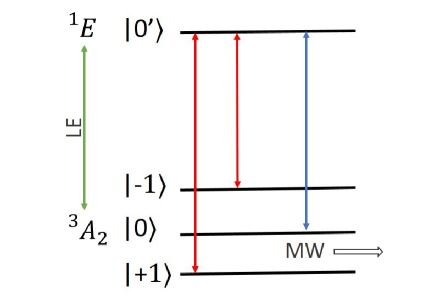
Figure 6: Scheme of NV^- center levels and the effective couplings. The ground state triplet and the meta-stable exited singlet state are coupled through a 532 nm laser field. The collective effects of optical excitation, de-excitation and non-radiative decay are similar to coupling the NV^- to hot (red arrows) and cold (blue arrow) thermal baths. Work is extracted in the form of amplifying a MW field that is in resonance with the transition $\left|+1\right>\leftrightarrow\left|0\right>$.

A microwave (MW) field set in resonance with the $\left|+1\right>\leftrightarrow\left|0\right>$ transition is then amplified, and power in the form of stimulated emission of MW radiation (maser) is extracted from the engine. The power is determined from a direct measurement of the fluorescence intensity change once the MW field is applied. This setup can be mapped to the three-level continuous engine discussed in detail in Sec. III.1.1. Since the level $\left|-1\right>$ is off-resonance with the MW field, it will not contribute to work extraction. Then the states $\{\left|+1\right>,\left|0\right>,\left|0^{\prime}\right>\}$ in Fig. (6) can be mapped to states $\{\left|1\right>,\left|2\right>,\left|3\right>\}$ of Fig. (5), where the level $\left|-1\right>$ only contributes to population transfer through level $\left|0^{\prime}\right>$. Switching on and off the MW field allows for the realization of a two-stroke engine and its comparison to the continuous engine.

The normalized action in this case Klatzow et al. (2017) is given by $\bar{s}=[\tfrac{\epsilon}{2}d+\gamma(1-d)]\tau_{cyc}$, where $\epsilon$ in Eq. (21) is twice the Rabi frequency, $\gamma$ is the total coupling rates to the baths and $d$ is the fraction of time of the work stroke out of the full cycle. Fig 7a presents a power measurement of a two-stroke engine that exceeds the stochastic bound set by Eq. (55). This is a clear indication of a quantum-thermodynamic signature in the operation of the engine. The stochastic bound, plotted in the purple line, was calculated for the parameters $\omega=2\pi\times 2600$ MHz, $\epsilon=3.2$ Mrad/s, $\gamma=0.41$ MHz, and $d=1/3$ while changing the cycle time $\tau_{cyc}$. The bound is violated by $2.4$ standard deviations. Fig. 7b demonstrates the equivalence principle in the form of Eq.(47). The powers of the two-stroke and continuous engines coincide in the small action regime. We also notice that, as predicted, the power of the continuous engine is independent of the cycle time. That is, for $\tau_{cyc}\rightarrow 0$ the power does not vanish as it would for a stochastic engine in the small action regime. This indicates that a continuous engine with the Hamiltonian structure (52) requires coherence in order to operate. In this experiment $\epsilon=5$ Mrad/s.

This experiment demonstrated the existence of quantum phenomena in microscopic thermal machines for the first time. In the small action regime, quantum coherence plays an important role in the operation of the engine. In this regime, the extracted power is enhanced, and thermodynamic properties of different types of engines coincide.

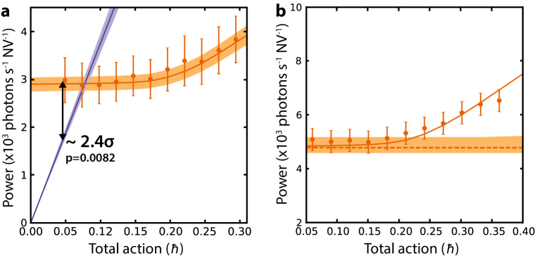
Figure 7: Power per NV^- center vs. the normalized action $\bar{s}$. (a) Quantum-thermodynamic signature: the orange line and data points present the theoretical and measured power of the two-stroke engine, respectively. The purple straight line is the upper stochastic bound on the power. In the small action regime, a clear violation of the stochastic bound (2.4 standard deviation) is observed. (b) The equivalence principle: The data points and the shaded region present power measurements of the two-stroke and continuous engines, respectively. The theoretical predictions for the two-stroke and continuous engines are given by the solid and dashed line, respectively. In the small action regime, the two measurements coincide. Figure courtesy of J. Klatzow, J. N. Becker, and E. Poem.

III.5 Quantum friction

Quantum friction is a quantum phenomenon that influences the operation of quantum thermal machines. It is related to the generation of coherences and excitations along a finite-time unitary evolution, and its dissipation when coupled to a thermal environment. Quantum friction in the context of quantum-theromodynamics was termed by Feldmann and Kosloff Feldmann and Kosloff (2000); Kosloff and Feldmann (2002) and is often referred as intrinsic or internal quantum friction. To understand this phenomenon intuitively, we will consider a specific example. We will compare two thermodynamic processes that will reveal the amount of energy lost to friction. The first process is an ideal quantum adiabatic process, where the initial state of the system is a thermal state $\rho_{i}=\exp[-\beta_{i}H_{i}]Z_{i}^{-1}$ with the initial inverse temperature $\beta_{i}$ and the initial Hamiltonian $H_{i}=H(0)$. The system is then driven adiabatically by changing the system energy scale and keeping its population constant. We require the final state to be expressed as $\rho_{f}=\exp[-\beta_{f}H_{f}]Z_{f}^{-1}$ such that $\beta_{f}$ is the inverse final temperature, $H_{f}=H(t_{f})$, and the final populations satisfy $P_{n}^{i}=P_{n}^{f}$. This requirement implies that for all $n$-levels, the compression ratio is given by $\epsilon_{n}^{f}/\epsilon_{n}^{i}=\beta_{i}/\beta_{f}$, where $\epsilon_{n}^{f,i}$ are the eigenvalues of $H_{f,i}$. This condition corresponds to Sec. II homogeneous energy scaling.

In real, finite-time processes, the adiabatic limit does not hold in general. Because of the non-commutativity of the Hamiltonian at different times, $[H(t),H(t^{\prime})]\neq 0$, coherences and excitations will be generated in the final state. Thus, we will consider a second, more real process. In the first stage the system is driven non-adiabaticaly by changing the Hamiltonian $H_{i}\rightarrow H_{f}$ so that at the end of this stage the system is found in some state $\rho_{\tau}$. In the second stage, the system is brought to equilibrium via coupling to a thermal bath at inverse temperature $\beta_{f}$ such that the final state is $\rho_{f}=\exp[-\beta_{f}H_{f}]Z_{f}^{-1}$. Such a process is elementary when studying quantum thermal machines, such as in the study of Carnot and Otto cycles. The energy that was invested in the creation of coherences and excitations and that was later dissipated to the thermal bath is the amount of energy lost to quantum friction.

In this sense, the effect of the non-adiabatic driving resembles the effect of friction in classical mechanics. Extra energy is needed to complete the process, which is then dissipated to the environment. The energy lost to friction is evaluated by the difference between the work invested in the real non-adiabatic stage and the work of the ideal adiabatic process,

$$W_{fric}=W_{re}-W_{ad}.$$ (56)

This amount of work is exactly the amount of energy dissipated (irreversibly) to the bath during the second stage of the second process. The work in the adiabatic process is $W_{ad}=tr(\rho_{f}H_{f})-tr(\rho_{i}H_{i})=\sum_{n}P_{n}^{i}(\epsilon_{n}^{f}-\epsilon_{n}^{i})$. For the non-adiabatic stage in the second process we have, $W_{re}=tr(\rho_{\tau}H_{f})-tr(\rho_{i}H_{i})$, implying that

$$W_{fric}=\sum_{n}\epsilon_{n}^{f}\left(\left<\epsilon_{n}^{f}\right|\rho_{\tau}\left|\epsilon_{n}^{f}\right>-P_{n}^{f}\right).$$ (57)

The work (57) can be related to the relative entropy of the final state $\rho_{\tau}$ at the end of stage one with the final thermal state $\rho_{f}$ at the end of stage two Plastina et al. (2014),

$$W_{fric}=\beta_{f}^{-1}S(\rho_{\tau}\parallel\rho_{f}).$$ (58)

To show this we, consider the the definition of the relative entropy

$$S(\rho_{\tau}\parallel\rho_{f}) = tr(\rho_{\tau}\ln\rho_{\tau})-tr(\rho_{\tau}\ln\rho_{f})=\sum_{n}P_{n}^{i}\ln P_{n}^{i}-\left(\left<\epsilon_{n}^{f}\right|\rho_{\tau}\left|\epsilon_{n}^{f}\right>-\ln P_{n}^{f}\right)$$

$$= \sum_{n}\beta_{f}\epsilon_{n}^{f}\left(\left<\epsilon_{n}^{f}\right|\rho_{\tau}\left|\epsilon_{n}^{f}\right>-P_{n}^{f}\right).$$

Here we used the fact that the von-Neumann entropy is invariant to unitary transformations, the relation $P_{n}^{i}=P_{n}^{f}$, and that $\ln P_{n}^{f}=-\beta_{f}\epsilon_{n}^{f}-\ln Z_{f}$. Since the relative entropy is non-negative, Eq. 58 implies that $W_{fric}\geq 0$. Applying arguments from Deffner and Lutz (2010) it was shown in Plastina et al. (2014) that a tighter bound for $W_{fric}$ can be obtained using the Bures length

$$W_{fric}\geq\frac{8\beta_{f}^{-1}}{\pi}L^{2}(\rho_{\tau},\rho_{f}),$$ (60)

where $L(\rho_{\tau},\rho_{f})=\text{arcos}(\sqrt{F(\rho_{\tau},\rho_{f})})$, with the fidelity $F(\rho_{\tau},\rho_{f})=\left[tr(\sqrt{\sqrt{\rho_{\tau}}\rho_{f}\sqrt{\rho_{\tau}}})\right]^{2}$.

More generally (i.e., not limited to the process above), the power along the work stroke of a thermal machine can be divided into classical and coherent extraction mechanisms Brandner et al. (2017)

$$P\equiv tr\left(\frac{dH(t)}{dt}\rho(t)\right)=\sum_{n}\dot{\epsilon}_{n}(t)\left<\epsilon_{n}(t)\right|\rho(t)\left|\epsilon_{n}(t)\right>+\left<\epsilon_{n}(t)\right|[H(t),\rho(t)]\left|\dot{\epsilon}_{n}(t)\right>.$$ (61)

The first term can be associated with classical power,

$$P_{clas}=\sum_{n}\dot{\epsilon}_{n}(t)\left<\epsilon_{n}(t)\right|\rho(t)\left|\epsilon_{n}(t)\right>=\sum_{n}\dot{\epsilon}_{n}(t)\rho_{nn}(t),$$ (62)

and the second term with the coherent power,

$$P_{coh}=\sum_{n}\left<\epsilon_{n}(t)\right|[H(t),\rho(t)]\left|\dot{\epsilon}_{n}(t)\right>=\sum_{n,l}(\epsilon_{n}-\epsilon_{l})\left<\epsilon_{l}|\dot{\epsilon}_{n}\right>\rho_{nl}(t),$$ (63)

where $\rho$ is expressed in the instantaneous eigenbasis of $H(t)$. Here, the term classical power is referred to power generated by changes in the energy levels of the engine and the contribution comes only from the diagonal terms of the density matrix in the energy basis. The contribution to the coherent power, however, arises only from the off-diagonal terms. The average classical and coherent work can be calculated by taking the time integral over the power. For the adiabatic process described above, $P_{coh}$ vanishes and the population $\rho_{nn}$ is fixed in time. Thus, the average work is again given by $\sum_{n}P_{n}^{i}(\epsilon_{n}^{f}-\epsilon_{n}^{i})$. Starting with a diagonal state in the energy basis, which often occurs after a full thermalization stroke, coherence will be generated once $[H(t),H(t^{\prime})]\neq 0$. Thus, $P_{coh}\neq 0$, and in general, the average coherent work will be non-zero. The terms “classical” and “coherent” in Eq. (62) and Eq. (63) should be used carefully. As we saw in the previous section, coherences and populations are coupled to each other during the dynamical evolution, so the distinction between the two may become ambiguous.

As long as dissipation is not introduced, friction is absent from the process, since the dynamic is reversible. In principle, one can extract all of the work from the state before it interacts with the thermal bath. By introducing a unitary cyclic process that transforms the state to a passive state Pusz and Wornwicz (1978), work can be extracted without changing the energy levels. This is the maximal amount of extractable work from a quantum state, and is sometimes referred to as ergotropy A. E. Allahverdyan, R. Balian, and Th. M. Nieuwenhuizen (2004). This procedure assumes that we have access to a semi-classical field and that the unitary operation can be implemented in practice.

Extracting work from coherences before they dissipate is one way to avoid friction. Other strategies to avoid friction in finite-time processes employ different control methods. Quantum lubrication Tova Feldmann and Ronnie Kosloff (2006) is a method that minimizes $S(\rho_{\tau}\parallel\rho_{f})$ in Eq. (58) by adding pure dephasing noise to the unitary stage. This additional noise can be considered as an instantaneous quantum Zeno effect, where the state of the system is projected to the instantaneous eigenstates of the time dependent Hamiltonian, eliminating the generation of coherence Levy et al. (2017). Shortcut to adiabaticity Torrontegui et al. (2013) are other useful control methods that can be essisted in order to find frictionless control Hamiltonians Xi Chen, A. Ruschhaupt, S. Schmidt, A. del Campo, D. Guery-Odelin, J. G. Muga (2010); Del Campo et al. (2014), which speed up adiabatic processes. For a given final time, the state of the system is an eigenstate of the final Hamiltonian $H_{f}$, but during the process, the state is subject to the generation of coherences and excitations. These control processes can be executed on very short time scales with high fidelity. If one assumes that the unitary evolution is not subject to noise from the control fields or from the environment, an exact frictionless Hamiltonian for finite time can be found. In a more realistic scenario where noise is present in the unitary process, one should aim to find a control Hamiltonian that minimizes the effect of noise Levy et al. (2018).

The average work measured by the energy difference between the end and the beginning of the process is the same for the shortcut to adiabticity protocol and the regular adiabatic process, which implies that frictionless protocols can in principle be implemented. However, in the shortcut protocol the instantaneous power can become very large and will require different resources in order to be implemented. Very fast protocols may require infinite resources. This is the manifestation of the time-power trade-off Levy et al. (2018) or the speed-cost trade-off Campbell and Deffner (2017). This feature was also recently studied by examining the growth of work fluctuations in shortcut protocols Funo et al. (2017).

IV Quantum correlations in the operation of thermal machines

The existence of quantum correlations is one of the most powerful signatures of non-classicality in quantum systems, as seen in recent reviews Modi et al. (2012); Horodecki et al. (2009) and references therein. In this context, thermodynamic approaches play a major role in witnessing and quantifying the existence of quantum correlations Oppenheim et al. (2002); Zurek (2003); Jennings and Rudolph (2010); Brodutch and Terno (2010); Popescu and Rohrlich (1997); Goold et al. (2016). Many studies relating thermodynamics with quantum correlation have focused on the amount of work extractable from correlations Alicki and Fannes (2013); Hovhannisyan et al. (2013); Perarnau-Llobet et al. (2015); Giorgi and Campbell (2015) or the thermodynamic cost of creating correlations Huber et al. (2015).

Quantum correlations have also been considered in the study of quantum thermal machines such as engines and refrigerators. In Brunner et al. (2014), entanglement between three qubits that form a quantum absorption refrigerator was studied. It was shown that near the Carnot bound entanglement is absent, nevertheless, in other regimes entanglement enhanced cooling and energy transport in the device. On the other hand, in a similar setup, that employed a different dynamical description of the refrigerator Luis A. Correa and Alonso (2013), it was shown that bipartite entanglement is absent between the qubits and correlations in the form of quantum discord which always exist in the system, do not influence the stationary heat flows. Entanglement in the working medium of quantum engines has mainly been investigated in the form of thermal-entanglement of two spins in Heisenberg types of models Zhang et al. (2007); Altintas et al. (2014); Wang et al. (2009); Huang et al. (2012). In these studies, the heat and the work produced by the engines are expressed in terms of the concurrence that measure the amount of entanglement in the system. Existence of temporal quantum correlations in a single two-level system Otto engine was also considered Friedenberger and Lutz (2017). It was shown that in some regimes of the engine operations, the Legget-Garg function exceeds its maximal classical value, which is a signature of non-classical behavior.

However, in most of the studies referred above, quantum correlations do not play a major role in the thermodynamic operation of the devices. The correlations were not exploited to gain power, and no clear quantum-thermodynamic signature is obtained. Instead, these studies only indicates that quantum correlation are present in the working medium when setting carefully the parameters of the problem. Next, we review a quantum-thermodynamic signature in the form of heat exchange. We believe this work will motivate further study on whether and how correlation can be exploited in the repeated operation of quantum thermal machines.

IV.1 Quantum-thermodynamic signatures

Here we derive a result obtained by Jennings and Rudolph Jennings and Rudolph (2010) on the average heat exchange between two local correlated thermal states. This study was motivated by the work of Parovi on the disappearance of the thermodynamic arrow in highly correlated environments Partovi (2008). Although the setup is not a standard thermal machine, which is the focus of this chapter, it can be considered as a single-shot cooling process where no external work is invested. Instead, correlations are exploited (as fuel) in order to cool the system. Moreover, this study presents an important thermodynamic signature of quantum-mechanical features that goes beyond what is possible classically. In the language of quantum information, the signature is called an entanglement witness. In particular, a bound on the amount of heat that can flow from a cold local thermal state to a hot local thermal state due to classical correlations is obtained. It is further shown that quantum correlations may violate this bound.

The Clausius statement of the second law of thermodynamics implies that when no work is done on the system, heat can only flow from a hotter body to colder body. This statement holds when no initial correlations are present between the two bodies. To show this, we consider two initially uncorrelated systems $A$ and $B$. The global initial state is thus represented by the product of the states of the two subsystems, $\rho_{AB}(0)=\rho_{A}(0)\otimes\rho_{B}(0)$. This is known as Boltzmann’s assumption of molecular chaos. We further assume that each subsystem is initially in a thermal state, $\rho_{X}(0)=\exp[-\beta_{X}H_{X}]$, where $X\in\{A,B\}$. Next we let the two subsystems interact via a global unitary interaction $U(\tau,0)$ for time $\tau$ that couples the two subsystems. As we wish to preserve the average energy of $\rho_{AB}$, and thus not perform any work on the system from external sources, we require that the transformation uphold $tr\left[\rho_{AB}(0)(H_{A}+H_{B})\right]=tr\left[\rho_{AB}(\tau)(H_{A}+H_{B})\right]$. After the interaction, the local reduced states are $\rho_{A,B}=tr_{B,A}(\rho_{AB})$ and the corresponding internal energy and entropy will change by the amount $\Delta E_{X}$ and $\Delta S_{X}$, where

$$\Delta E_{X} = tr\left[(\rho_{X}(\tau)-\rho_{X}(0))H_{X}\right],$$ (64)

$$\Delta S_{X} = S_{X}(\tau)-S_{X}(0),$$

and $S_{X}=-tr(\rho_{X}\ln\rho_{X})$ is the von-Neumann entropy. Since the thermal state minimizes the free energy, $F(\rho_{X})=tr\left[\rho_{X}H_{X}\right]-S(\rho_{X})/\beta_{X}$, we obtain, $tr\left[\rho_{X}(0)H_{X}\right]-S(\rho_{X}(0))/\beta_{X}\leq tr\left[\rho_{X}(\tau)H_{X}\right]-S(\rho_{X}(\tau))/\beta_{X}$, which can be cast into Peres (2006)

$$\beta_{X}\Delta E_{X}-\Delta S_{X}\geq 0.$$ (65)

To quantify the amount of correlations present between the two subsystems $A$ and $B$ we will use the quantum mutual information for bipartite systems:

$$I_{q}[\rho_{AB}]\equiv S(\rho_{AB}\parallel\rho_{A}\otimes\rho_{B})=S_{A}+S_{B}-S_{AB}.$$ (66)

This function is always non-negative Wehrl (1978) and accounts for both classical and quantum correlations. For product states, like the one considered in the process above, the mutual information vanishes, $I_{q}[\rho_{AB}(0)]=0$. This implies that at time $\tau$ the change in the mutual information is $\Delta I_{q}[\rho_{AB}]=I_{q}[\rho_{AB}(\tau)]\geq 0$. On the other hand since $S_{AB}$ is invariant under the unitary transformation $U(\tau,0)$ we obtain $\Delta I_{q}[\rho_{AB}]=\Delta S_{A}+\Delta S_{B}$ which is true irrespective of the initial conditions. Applying these relation to (65) we obtain

$$\beta_{A}Q_{A}+\beta_{B}Q_{B}\geq\Delta I_{q}(\rho_{AB})\geq 0,$$ (67)

where we identified the heat transferred to system $X$ as the change in its internal energy, $Q_{X}=\Delta E_{X}$. Since $Q_{A}=-Q_{B}$, relation (67) implies that heat will always flow from hot to cold. Note, however, if the assumption of initial product state is removed then $\Delta I_{q}[\rho_{AB}]$ can become negative, which opens up the possibility of “anomalous heat flow” namely heat flowing from the colder body to the hotter body. In this case Eq. (67) reads

$$\beta_{A}Q_{A}+\beta_{B}Q_{B}\geq-|\Delta I_{q}(\rho_{AB})|.$$ (68)

The initial correlations present in the system, which can be either classical, quantum, or both, are the source of this backward flow. In order to derive a clear quantum-thermodynamic signature, a bound on the maximal backward flow that could occur from just classical correlations is set. The classical mutual information of a quantum state is given by taking the maximum over all POVMs $M_{A}\otimes M_{B}$, which are the most general kind of quantum measurements possible on $A$ and $B$ Terhal et al. (2002):

$$I_{c}(\rho_{AB})=\max_{M_{A}\otimes M_{B}}\left[H(P_{A})+H(P_{B})-H(P_{AB})\right],$$ (69)

where $H(P)$ is the Shannon entropy of the measurement statistics $P$. The classical mutual information satisfies $0\leq I_{c}(\rho_{AB})\leq I_{q}(\rho_{AB})$ Lindblad (1974), which implies that $\max|\Delta I_{c}(\rho_{AB})|\leq\max|\Delta I_{q}(\rho_{AB})|$. To obtain a bound on $\max|\Delta I_{c}(\rho_{AB})|$ that is independent of the specific details of the states, we note that $I_{c}(\rho_{AB})\leq\ln D$, where $D=\min\{\text{Dim}(\rho_{A}),\text{Dim}(\rho_{B})\}$ is the dimension of the smaller system. This bound is a result of the monotonicity property of the Shannon entropy under partial trace, $H(P_{AB})\geq H(P_{A}),H(P_{B})$. The same argument applies for the von-Neumann entropy for separable states $S(\rho_{AB}|_{\text{sep}})\geq S(\rho_{A}),S(\rho_{B})$ Horodecki and Horodecki (1994). The upper bound, $\ln D$, is saturated for perfectly correlated, zero discord, separable states $\rho_{AB}=\tfrac{1}{D}\sum_{k}\left|e_{k}\right>\left<e_{k}\right|_{A}\left|f_{k}\right>\left<f_{k}\right|_{B}$, where $\left|e_{k}\right>$ and $\left|f_{k}\right>$ are orthonormal bases for A and B. Assuming that the initial state $\rho_{AB}$ is the perfectly correlated state above and that at the final time it is a product state, the maximal violation of heat transfer from cold to hot due to classical correlations is

$$Q_{clas}=\frac{\ln D}{|\beta_{A}-\beta_{B}|}.$$ (70)

Since for entangled states the mutual entropy can exceed $\ln D$, and in fact, go to $2\ln D$ for maximally entangled states, the violation of heat transfer can exceed $Q_{clas}$. Thus, any measurement of heat exchange that gives $Q>Q_{clas}$ indicates that the initial state $\rho_{AB}$ was necessarily entangled. Therefore the heat-flow pattern acts as a “witness” that reveals genuine non-classicality in the thermodynamic system. Moreover, this quantum resource can be exploited in a cooling process, removing heat from a colder body and transfer it to a hotter one. This phenomenon was recently demonstrated in a NMR experiment Micadei et al. (2017), where it was shown that heat is transferred from a colder nuclear spin to a hotter one due to correlations. The result presented here was later extended to derive an exchange fluctuation theorem for energy exchange between thermal quantum systems beyond the assumption of molecular chaos Jevtic et al. (2015).

V Conclusions

In this chapter we have presented a short review about some of the studies that compare the performance of classical and quantum heat machines. In particular, we have focused on three main quantum features, energy quantization, quantum coherence, quantum correlations, and their manifestation in the operation of quantum thermal machines. All of these features boil down to the mathematical structure of quantum mechanics, which is represented by wave functions and operators acting in Hilbert space. However, we showed that the manifestation of particular quantum phenomena can be distinguished from one another. Specifically, we saw that energy quantization and the uncertainty principle alone lead to differences in the behavior of heat engines. Moreover, quantum mechanics enables the realization of thermal-machines with incompressible working medium which is classically impossible.

The role of quantum coherence was also studied. Since the generation of coherences for interacting quantum systems is typically unavoidable, and since coherences have thermodynamic cost, dephasing leads to quantum friction. Working in the small action regime, complete dephasing can be suppressed. In this regime, coherences survive the couplings to the thermal baths, and quantum engines outperform stochastic engines, which incorporate only populations in their operation. This phenomenon can be observed experimentally by setting a bound on the maximal power obtained by a stochastic engine. A violation of this bound is a signature of a quantum-thermodynamic behavior. Furthermore, in the small action regime, the thermodynamic properties of different types of engines coincide, since coherent work extraction becomes dominant.

Quantum correlations are obviously closely related to the existence of coherence between particles, however, by investigating bounds on classically correlated systems, it is possible to isolate the effects of quantum correlations. Here, we demonstrated that the presence of quantum correlations can explain anomalous heat flow that cannot be achieved classically.

As we have shown, operating in the quantum regime is not always advantageous. Thus it is important to understand the quantum behavior of thermal-machines in order to avoid undesired reductions in the performance. We believe that the results presented here represent only some initial results that require further investigation, such as:

• What are the features needed on the potentials for providing a quantum boost to the work and heat exchange and how do these features relate to other quantum proprieties?

• One possible manner of obtaining an efficiency divergence between classical and quantum heat machines is by performing a thermal cycle that involves an inhomogeneous energy level scaling. As of today, there are only a small number of studies concerned with this type of cycle, calling for further research in this direction.

• Since coupling to a thermal source is an elementary process in thermal devices, innovative methods to exploit quantum coherences and correlations before they decay are essential for obtaining quantum supremacy. Possible approaches are: identifying and operating in the regime where the quantum effects are still relevant; applying quantum control methods, such as feedback control, in order to maintain the quantum properties.

• The main results concerning the relationship between thermodynamics and quantum correlations are focused on single-shot processes. A desired goal would be to exploit correlations in the repeated operation of a device.

• Can the quantum thermal-machines be scaled up in size and maintain their quantum nature? Can we deduce from these models something about energy transfer and quantum behavior of more complex systems, such as biological systems?

As we have shown, the actual performances of classical and quantum heat machine diverge, even though both are limited by the same fundamental thermodynamic bounds, such as the Carnot efficiency. Nevertheless, the difference between them is noteworthy and should be studied further, especially considering the fast experimental progress that has already succeeded in demonstrating quantum behavior of thermal-machines.