Calculation of interatomic forces and optimization of molecular geometry with auxiliary-field quantum Monte Carlo

Abstract

We propose an algorithm for accurate, systematic and scalable computation of interatomic forces within the auxiliary-field Quantum Monte Carlo (AFQMC) method. The algorithm relies on the Hellman-Fenyman theorem, and incorporates Pulay corrections in the presence of atomic orbital basis sets. We benchmark the method for small molecules by comparing the computed forces with the derivatives of the AFQMC potential energy surface, and by direct comparison with other quantum chemistry methods. We then perform geometry optimizations using the steepest descent algorithm in larger molecules. With realistic basis sets, we obtain equilibrium geometries in agreement, within statistical error bars, with experimental values. The increase in computational cost for computing forces in this approach is only a small prefactor over that of calculating the total energy. This paves the way for a general and efficient approach for geometry optimization and molecular dynamics within AFQMC.

Calculating interatomic forces in molecules is important for a quantitative understanding of their physical properties. Forces are the basic ingredient in a variety of fundamental studies including molecular dynamics simulations Car_PRL55_1985 , optimization of molecular geometries Pulay_MP17_1969 ; Eckert_JCC18_1997 ; Pulay_WIRES4_2014 , computation of vibrational properties Pulay_WIRES4_2014 and reaction path following Eckert_TCA100_1998 .

Despite the incredible success within the framework of density functional theory (DFT) Reveles_JCC25_2004 , much effort has been devoted to developing many-body schemes that can describe more accurately physical and chemical situations where DFT is less reliable, for instance in cases of large electronic correlations and long-range dispersive forces Busch_JCP94_1991 ; Azhary_JCP108_1998 ; Rauhut_PCCP3_2001 . Quantum Monte Carlo (QMC) methods are one of the promising alternative many-body approaches, which treat electronic correlations by stochastically sampling of correlated wavefunctions.

The auxiliary-field quantum Monte Carlo (AFQMC) method Zhang_PRL90_2003 , in particular, has seen rapid development and applications to a wide variety of quantum chemistry and condensed-matter systems AlSaidi_JCP124_2006 ; Suewattana_PRB75_2007 ; Purwanto_JCP128_2008 ; Purwanto_JCP130_2009 ; Purwanto_JCP142_2015 ; Purwanto_JCP144_2016 ; Kwee_PRL100_2008 ; Purwanto_PRB80_2009 ; Ma_PRL114_2015 ; Shee2017 , yielding state-of-the-art, benchmark-quality results Motta_PRX_2017 for the energies of ground and excited states. It is intrinsically parallel, having tremendous capacity to take advantage of petascale (and bebyond) computing resources Esler_JP125_2008 . The computational cost scales as the third or fourth power of the system size, offering the potential to treat large many-electron systems.

The calculation of forces with QMC methods has been a long standing problem Zong_PRE58_1998 ; Casalegno_JCP118_2003 ; Lee_JCP122_2005 ; Sorella_JCP133_2010 . Despite significant recent development Assaraf_JCP113_2000 ; Assaraf_JCP119_2003 ; Filippi_PRB61_2000 ; Casalegno_JCP118_2003 ; Chiesa_PRL94_2005 ; Moroni_JCTC10_2014 , computing forces reliably and efficiently beyond variational Monte Carlo (VMC) methods has remained a major challenge.

In this paper, we present an algorithm to directly calculate interatomic forces within AFQMC. As the AFQMC algorithm works by sampling a non-orthogonal Slater determinant space, its formalism allows the adaptation of several key ingredients from other electronic structure or quantum chemistry methods. Combining this with recent advances in the back-propagation technique Motta_JCTC_2017 , we achieve an efficient approach for computing atomic forces within AFQMC. In this paper we describe the algorithm, and demonstrate it by full QMC geometry optimization in molecules using a simple steepest descent approach. Internal consistency of the algorithm is verified by measuring the agreement between computed forces and the gradients of the potential energy surface. We benchmark the accuracy of the algorithm by comparison with available high-level quantum chemistry and/or experimental results.

The AFQMC method Zhang_PRL90_2003 ; Zhang_notes_2013 ; Motta_WIRES_2017 reaches the many-body ground state $\Psi_{0}$ of a Hamiltonian $\hat{H}$ by an iterative process, $|\Psi_{0}\rangle\propto\lim_{n\to\infty}\exp(-n\,\Delta\tau\hat{H})\,|\Psi_{T}\rangle$, where $\Delta\tau$ is a small parameter and, for convenience, we take the initial state $\Psi_{T}$, which must be non-orthogonal to $\Psi_{0}$, to be a single Slater determinant. The many-body propagator is written as

$$e^{-\Delta\tau\hat{H}}=\int d{\bf{x}}\,p({\bf{x}})\,\hat{B}({\bf{x}})\,,$$ (1)

where $\hat{B}({\bf{x}})$ is an independent-particle propagator that depends on the multi-dimensional vector ${\bf{x}}$, and $p({\bf{x}})$ is a probability distribution function Zhang_PRL90_2003 . AFQMC thus represents the many-body wave function in the iteration as an ensemble of Slater determinants,

$$\begin{split}|\Psi^{(n)}\rangle&=e^{-n\,\Delta\tau\hat{H}}|\Psi_{T}\rangle\propto\int d\Psi\,\lambda_{n}(\Psi)|\Psi\rangle\,,\\ \lambda_{n}(\Psi)&=\int\prod_{l=0}^{n-1}d{\bf{x}}_{l}\,\,p({\bf{x}}_{l})\,\,\delta\left(\Psi,\prod_{l=0}^{n-1}\hat{B}({\bf{x}}_{l})\Psi_{T}\right)\,,\end{split}$$ (2)

where $\int d\Psi$ denotes integration over the manifold of Slater determinants $\Psi$ Fahy_PRB43_1991 .

The ground-state expectation value of an operator $\hat{A}$ can be obtained as

$$\frac{\langle\Psi^{(m)}|\hat{A}|\Psi^{(n)}\rangle}{\langle\Psi^{(m)}|\Psi^{(n)}\rangle}=\frac{\int d\Phi d\Psi\,\rho_{m,n}(\Phi,\Psi)\,W(\Phi,\Psi)\,A_{loc}(\Phi,\Psi)}{\int d\Phi d\Psi\,\rho_{m,n}(\Phi,\Psi)\,W(\Phi,\Psi)}\,,$$ (3)

in the limit of large $n$ and $m$, where $\rho_{m,n}(\Phi,\Psi)=\mu^{*}_{m}(\Phi)\lambda_{n}(\Psi)$. Formally $\mu_{m}$ in the distribution $\rho$ should be the same as $\lambda_{m}$; however, we have used a different symbol to emphasize that in AFQMC the paths leading to it are obtained by the back-propagation algorithm Purwanto_PRE70_2004 ; Motta_JCTC_2017 . Operationally this can be thought of as generating $N_{w}$ Monte Carlo (MC) path configurations of auxiliary fields, $\{{\bf{x}}_{0},{\bf{x}}_{1},\cdots,{\bf{x}}_{n-1};{\bf{x}}_{n},\cdots,{\bf{x}}_{n+m-1}\}$, in the stochastic sampling of $\langle\Psi^{(m)}|\Psi^{(n)}\rangle=\langle\Psi_{T}|\Psi^{(n+m)}\rangle$, and then back-propagate $\langle\Psi_{T}|$ for $m$ steps along the path to obtain $\langle\Psi^{(m)}|$,

$$\mu_{m}(\Phi)=\int\prod_{l=n}^{n+m-1}d{\bf{x}}_{l}\,\,p({\bf{x}}_{l})\,\,\delta\left(\Phi,\prod_{l=n+m-1}^{n}\hat{B}({\bf{x}}_{l})^{\dagger}\Psi_{T}\right)\,.$$ (4)

In Eq. (3), $|\Psi\rangle$ and $\langle\Phi|$ in the overlap $W(\Phi,\Psi)=\langle\Phi|\Psi\rangle$ and the local expectation $A_{loc}(\Phi,\Psi)=\langle\Phi|\hat{A}|\Psi\rangle/\langle\Phi|\Psi\rangle$ are defined on the path at “time-slices” $(n-1)$ and $n$, respectively. The expectation is evaluated over the MC samples (labeled by $w$) as

$$\frac{\langle\Psi_{0}|\hat{A}|\Psi_{0}\rangle}{\langle\Psi_{0}|\Psi_{0}\rangle}\simeq\frac{\sum_{w=1}^{N_{w}}W(\Phi_{w},\Psi_{w})\,A_{loc}(\Phi_{w},\Psi_{w})}{\sum_{w=1}^{N_{w}}W(\Phi_{w},\Psi_{w})}\,.$$ (5)

Because the propagator $\hat{B}({\bf{x}})$ contains stochastically fluctuating fields, the MC sampling will lead to negative (indeed complex) overlaps $W$, which will cause the variance of this estimator to grow exponentially with the projection times, $n$ and $m$. Control of this phase problem is achieved by the introduction of an importance sampling transformation and a generalized gauge condition to constrain the random walks Zhang_PRL90_2003 .

This framework eliminates the phase problem, at the cost of modifying the distribution $\rho_{m,n}$. The constraint introduces a bias in $\lambda_{n}$. For $\mu_{m}$ an additional subtlety arises because the constraint on the path is imposed in the time-reversed direction Motta_WIRES_2017 . Previous studies in a variety of systems have shown that the bias from the constraint tends to be small, in both models LeBlanc_PRX5_2015 and realistic materials Motta_PRX_2017 , making AFQMC of the most accurate many-body approaches for general interacting fermion systems.

To address the problem of computing atomic forces, let us consider a molecule comprising $N_{n}$ ions, whose spatial positions ${\bf{R}}=({\bf{R}}_{1}\dots\bf{R}_{N_{n}})$ define a molecular geometry. Given a molecular geometry ${\bf{R}}$, ground-state expectation values of physical observables are given by

$$A({\bf{R}})=\frac{\langle\Psi_{0}({\bf{R}})|\hat{A}({\bf{R}})|\Psi_{0}({\bf{R}})\rangle}{\langle\Psi_{0}({\bf{R}})|\Psi_{0}({\bf{R}})\rangle}\equiv\mathcal{A}[\rho_{m,n};{\bf{R}}]\,.$$ (6)

For $\hat{A}({\bf{R}})=\hat{H}({\bf{R}})$, Eq. (6) gives the potential energy surface (PES), $E({\bf{R}})$. The gradient of (6) is in general given by

$$\frac{\partial A}{\partial R_{\alpha}}=\frac{\partial\rho_{m,n}}{\partial R_{\alpha}}\frac{\partial\mathcal{A}}{\partial\rho_{m,n}}+\frac{\partial\mathcal{A}}{\partial R_{\alpha}}\,.$$ (7)

In the case of the PES, the first two terms vanish for sufficiently large $m$ and $n$. However, the expression does not reduce to Hellmann-Feynman theorem Hellmann_book_1937 ; Feynman_PR56_1939 , because $\Psi$ and $\Phi$ are represented by incomplete atom-centered basis sets which depend on ${\bf{R}}$. Performing the partial derivative in Eq. (3), one obtains

$$\begin{split}&F^{\alpha}({\bf{R}})=\frac{\partial E}{\partial R_{\alpha}}({\bf{R}})=\\ =\,&\frac{\int d\Phi d\Psi\,\rho_{m,n}(\Phi,\Psi)\,W(\Phi,\Psi;{\bf{R}})\,F^{\alpha}_{loc}(\Phi,\Psi;{\bf{R}})}{\int d\Phi d\Psi\,\rho_{m,n}(\Phi,\Psi)\,W(\Phi,\Psi;{\bf{R}})}\,,\end{split}$$ (8)

with

$$\begin{split}&F^{\alpha}_{loc}(\Phi,\Psi;{\bf{R}})=\frac{\partial E_{loc}}{\partial R_{\alpha}}(\Phi,\Psi;{\bf{R}})\\ +\,&\frac{\partial_{R_{\alpha}}W(\Phi,\Psi;{\bf{R}})}{W(\Phi,\Psi;{\bf{R}})}\big{(}E_{loc}(\Phi,\Psi;{\bf{R}})-E({\bf{R}})\big{)}\,.\end{split}$$ (9)

The terms in Eq. (9) are detailed in the Appendix, and encompass a Pulay’s correction Pulay_MP17_1969 to take into account the explicit dependence of the one-electron Green’s function on atomic coordinates ${\bf{R}}$.

Ground-state expectation values of the form in Eq. (LABEL:eq:gradient) can be computed accurately with the back-propagation algorithm, originally formulated for lattice models of correlated electrons Zhang_PRB_1997 , generalized to weakly correlated systems with complex $\hat{B}({\bf x})$ Purwanto_PRE70_2004 , and recently adapted to molecular systems with a “path restoration” (BP-PRes) technique Motta_JCTC_2017 . The computational cost of evaluating $F^{\alpha}_{loc}(\Phi,\Psi;{\bf{R}})$ is similar to that of computing the local energy. Additional speedup can be achieved by exploiting the local nature of the atomic forces and the sparsity of the Hamiltonian matrix elements. In larger molecules and solids, the ability to evaluate all forces simultaneously (as opposed to separate total energy calculations for each force component) is crucial, and paves the way for geometry optimizations.

We note that the formalism and estimator detailed above hold for any other method operating in an overcomplete manifold of non-orthogonal Slater determinants. Differences arise in the generation of the distributions $\mu$ and $\lambda$ which, as discussed above, need not be differentiated to compute the atomic forces.

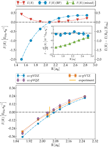
Figure 1: (color online) Top: AFQMC potential energy surface $E(R)$ (red triangles) and computed force $F(R)$ (blue points) of CH₄ as function of the CH bondlength $R$ (cc-pVDZ basis). The minimum of the energy $E(R)$ is attained when $F(R)=0$, as expected. Inset: comparison between computed force $F(R)$ using back-propagation (blue points) and mixed estimator, i.e. $m=0$ in Eq. (3) (green triangles), and numerical finite difference of $dE(R)/dR$, taken as reference. Bottom: AFQMC computed force $F(R)$ of CH₄, using cc-pVxZ basis sets.

In Fig. 1 we assess the internal consistency and accuracy of our method using the symmetric stretching of the CH bond in CH₄ as a test case. The computed gradients, across the entire bondlength range, are in agreement with results from explicit (numerical) derivative of the PES within statistical uncertainties. As the inset in the upper panel illustrates, it is crucial to have BP in order for Eq. (LABEL:eq:gradient) to achieve an accurate representation of Eq. (7). Performing calculations with increasingly large basis sets, we observe convergence of the equilibrium bondlength to the complete basis set (CBS) limit ($R=2.0844(32)$, $2.0605(70)$, $2.0458(62)\,\mathrm{a_{B}}$ at cc-pVDZ, TZ, QZ level respectively), and good agreement with the experimental equilibrium bondlength ($R=2.0541(19)\,\mathrm{a_{B}}$ CCCBDB2016 ).

As a further test, we perform a geometry optimization in Fig. 2 for the H₂O molecule using the steepest-descent algorithm. The computed equilibrium geometry is in agreement with the global minimum of the PES, obtained from AFQMC calculations of the ground-state energy on a dense mesh of points. In Table 1 we list the optimized geometries for different basis sets, together with those from the coupled-cluster CCSD(T) for comparison and benchmark. The statistical error bars on the QMC geometry are obtained by averaging over configurations of $\{{\bf{R}}_{i}\}$ with converged and statistically compatible energies, for example, at the cc-pVDZ level, $i=6\dots 11$ (see bottom panel in Fig. 2). From Table 1, convergence to the CBS limit is seen at the cc-pVQZ level, where the AFQMC results are in good agreement with experiment CCCBDB2016 .

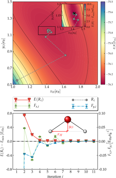
Figure 2: (color online) Top: The PES, $E({\bf{R}})$, computed on a dense mesh from AFQMC (color plot) and steps (gray points) of a steepest-descent geometry optimization for H₂O, at cc-pVDZ level. Inset: magnified view around the equilibrium geometry. The location of the global minimum of PES is indicated with a cross ($x_{H}=1.4179(12)\,\mathrm{a_{B}}$, $y_{O}=1.1593(12)\,\mathrm{a_{B}}$). Bottom: convergence of the AFQMC energy $E({\bf{R}}_{i})$ and extinction of the residual forces $F_{x,i}=\partial E({\bf{R}}_{i})/\partial x_{H}$ (green diamonds) and $F_{y,i}=\partial E({\bf{R}}_{i})/\partial y_{O}$ (blue squares) during the steepest-descent geometry optimization. The relevant geometry parameters $x_{H}$ and $y_{O}$ are sketched.

basis	method	$x_{H}$ [$\mathrm{a_{B}}$]	$y_{O}$ [$\mathrm{a_{B}}$]
cc-pVDZ	CCSD(T)	1.418	1.149
	AFQMC	1.414(2)	1.158(1)
cc-pVTZ	CCSD(T)	1.424	1.118
	AFQMC	1.426(3)	1.121(4)
cc-pVQZ	CCSD(T)	1.439	1.109
	AFQMC	1.425(5)	1.098(4)
	experiment	1.431	1.108

Table 1: Equilibrium geometries of H₂O computed from AFQMC with several basis sets, compared to the corresponding CCSD(T) result and experimental CCCBDB2016 equilibrium geometries. The geometry is defined in terms of two parameters $x_{H}$ and $y_{O}$, as sketched in Fig. 2.

In Fig. 3 we move to the more challenging case of ethane. Geometries respecting the $\mathrm{D_{3}h}$ symmetry of the molecule can be expressed in terms of $3$ parameters, as sketched in the inset. As the number of geometric parameters grows, it quickly becomes impractical to compute the entire PES with AFQMC as was done in Fig. 2, and forced-based methods become essential. The optimized parameters, with the modest but realistic cc-pVDZ basis, are within 0.02 a.u. (or 1%) of the experimental equilibrium geometry, as seen in Table 2. The excellent agreement between the AFQMC geometry and those from high-level QC methods at this basis level suggests that the discrepancy with experimental data is likely a result of basis set incompleteness, which is quantitatively confirmed by a cc-pVTZ calculation. The ground-state energies computed at the optimized geometry and at the experimental equilibrium geometry are in agreement with each other: $E({\bf R}_{\rm op})-E({\bf R}_{\rm eq})=-0.5(4)$ mHa.

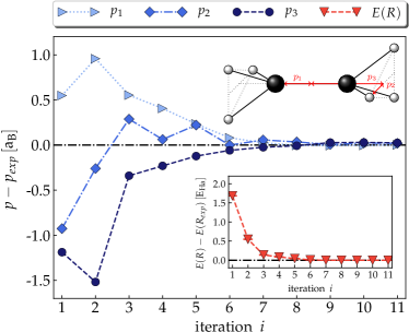
Figure 3: (color online) Evolution of the molecular geometry for ethane during an AFQMC geometry optimization with the steepest descent algorithm. (The cc-pVDZ basis set was used here.) The inset shows the corresponding total energy.convergence. Molecular geometries are expressed in terms of $3$ parameters, ${\bf{R}}={\bf{R}}({\bf{p}})$, as sketched in the upper right corner.

basis	method	$p_{1}\,[\mathrm{a_{B}}]$	$p_{2}\,[\mathrm{a_{B}}]$	$p_{3}\,[\mathrm{a_{B}}]$
cc-pVDZ	DFT-B3LYP	1.4447	1.9393	2.2080
	QCISD(TQ) CCCBDB2016	1.4513	1.9496	2.2079
	CCSD(T)	1.4498	1.9476	2.2061
	AFQMC	1.448(2)	1.947(6)	2.205(8)
cc-pVTZ	DFT-B3LYP	1.4430	1.9202	2.1941
	QCISD(TQ) CCCBDB2016	1.4456	1.9271	2.1902
	CCSD(T)	1.4391	1.9183	2.1803
	AFQMC	1.443(5)	1.912(8)	2.192(6)
	experiment CCCBDB2016	1.4513	1.9260	2.1869

Table 2: Equilibrium geometries of ethane from AFQMC. Results with the cc-pVDZ basis set are compared with several other QC methods. Results from cc-pVTZ indicate reasonable convergence with respect to basis set, and good agreement with experiment. DFT and CCSD(T) data were computed using the NWChem software Valiev_CPC_2010 . Geometries are expressed in terms of the parameters $p_{1}$, $p_{2}$, $p_{3}$ sketched in Fig. 3.

As a last example, we optimize the molecular geometry of nitric acid. We use increasingly larger basis sets to reach the continuum limit near the optimal geometry. As shown in Fig. 4, there is a large residual error in the STO-6G basis set, and the optimized geometry is significantly different from experiment. As more realistic basis sets are employed, systematically improved results are obtained, and the computed geometry approaches the experimental equilibrium geometry. At the cc-pVTZ level, AFQMC results are in agreement with experiment to within 0.01 a.u.

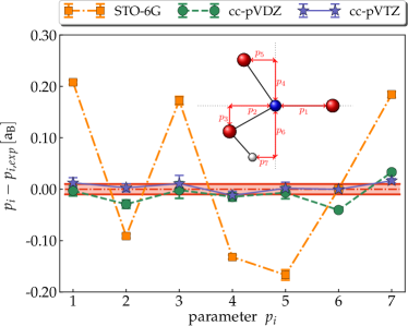
Figure 4: (color online) Optimization of nitric acid with AFQMC. The deviation between the final optimized geometry and the experimental equilibrium geometry is shown for each basis set ( STO-6G, cc-pVDZ and cc-pVTZ). The pink band indicates a range within 0.01 a.u. of experimental values.

We have demonstrated the direct computation of interatomic forces and molecular geometry optimization within AFQMC. We proposed an internally consistent, numerically stable and computationally efficient algorithm based on the Hellman-Feynman theorem and Pulay’s corrections. Results from a first application are presented. Accurate forces are obtained using simple RHF Slater determinant as constraining trial wave function. These results pave the way for systematic geometry optimization and potentially molecular dynamics using one of the most accurate many-body methods with low-power computational scaling.

A variety of future directions are possible, including both applications and further generalization and improvement of the algorithm. More refined Ansätze Purwanto_JCP130_2009 ; Purwanto_JCP142_2015 ; Purwanto_JCP144_2016 for the trial wave function can be adopted straightforwardly for more challenging molecules. Interfacing with better optimization strategies and improving the efficiency of the force computation algorithm with AFQMC itself can both lead to major increases in the capability of the method. Alternative representations Purwanto_JCP135_2011 ; Ma_PRL114_2015 of the Hamiltonian operator should be explored. Applications to a variety of molecular systems are within reach including those containing post-second-row elements. Geometry optimization in crystalline solids is being investigated.

We acknowledge support by NSF (Grant no. DMR-1409510), DOE (Grant no. DE-SC0001303), and the Simons Foundation. Computations were carried out at the Extreme Science and Engineering Discovery Environment (XSEDE), which is supported by National Science Foundation grant number ACI-1053575, at the Storm and SciClone Clusters at the College of William and Mary. M. M. acknowledges James Shee and Qiming Sun for valuable interaction.

Appendix A AFQMC estimator of interatomic forces

The starting point for the evaluation of forces is the general form of the ground-state expectation value of the Hamiltonian operator,

$$E({\bf{R}})=\frac{\int d\Phi d\Psi\,\rho_{m,n}(\Phi,\Psi)\,W(\Phi,\Psi;{\bf{R}})\,E_{loc}(\Phi,\Psi;{\bf{R}})}{\int d\Phi d\Psi\,\rho_{m,n}(\Phi,\Psi)\,W(\Phi,\Psi;{\bf{R}})}\,.$$ (10)

The Slater determinant $|\Psi\rangle=\prod_{\sigma}\prod_{l=1}^{N_{\sigma}}\psi_{l\sigma}^{\dagger}|\emptyset\rangle$ has $N_{\sigma}$ ($\sigma=\uparrow$ or $\downarrow$) fermions occupying orbitals $|\psi_{l\sigma}\rangle\equiv\psi_{l\sigma}^{\dagger}|\emptyset\rangle=\sum_{i}\left(C_{\Psi,\sigma}\right)_{il}|\chi_{i}\rangle$, where $\{|\chi_{i}\rangle,i=1\dots M\}$ are the basis functions and $C_{\Psi,\sigma}$ is a $M\times N_{\sigma}$ matrix that contains the orbital coefficients. The Slater determinant $|\Phi\rangle$ is similarly defined in terms of orbitals $|\phi_{l\sigma}\rangle$ and matrix $C_{\Phi,\sigma}$. In Eq. (10), the overlap is given by

$$\begin{split}&W(\Phi,\Psi;{\bf{R}})\equiv\langle\Phi|\Psi\rangle\\ =&\prod_{\sigma}\mbox{det}\left(C_{\Phi,\sigma}^{\dagger}S({\bf{R}})C^{\phantom{\dagger}}_{\Psi,\sigma}\right)\equiv\prod_{\sigma}\mbox{det}\left(\Omega_{\sigma}({\bf{R}})\right)\,,\end{split}$$ (11)

where $S({\bf{R}})_{ij}=\langle\chi_{i}|\chi_{j}\rangle$ is the overlap matrix of the AO basis set. The local energy is given by

$$\begin{split}E_{loc}(\Phi,\Psi;{\bf{R}})=H_{0}({\bf{R}})+\sum_{\sigma}\mbox{Tr}[h({\bf{R}})G_{\sigma}({\bf{R}})]+\sum_{\gamma}\Big{(}\sum_{\sigma}\mbox{Tr}[L^{\gamma}({\bf{R}})G_{\sigma}({\bf{R}})]\Big{)}^{2}-\sum_{\sigma}\mbox{Tr}[L^{\gamma}({\bf{R}})G_{\sigma}({\bf{R}})L^{\gamma}({\bf{R}})G_{\sigma}({\bf{R}})]\,,\end{split}$$ (12)

where $H_{0}({\bf{R}})$ is a constant from the internuclear repulsion, the matrix $h({\bf{R}})$ is the one-body part of the Hamiltonian in the AO basis ($h({\bf{R}})_{ij}=\langle\chi_{i}|h_{1}({\bf{R}})|\chi_{j}\rangle$), the matrices $L^{\gamma}({\bf{R}})$ arise from decomposing the two-body part of the Hamiltonian (e.g., via the Cholesky or density-fitting decomposition Purwanto_JCP135_2011 ; Sun_arxiv_2017 , $(ik|jl)=\sum_{\gamma}L^{\gamma}({\bf{R}})_{ik}L^{\gamma}({\bf{R}})_{jl}$), and the (spin-dependent) one-electron Green’s function is

$$G_{\sigma}({\bf{R}})=C^{\phantom{\dagger}}_{\Psi,\sigma}\Omega_{\sigma}({\bf{R}})^{-1}C_{\Phi,\sigma}^{\dagger}\,,$$ (13)

which obeys the idempotence relation

$$G_{\sigma}({\bf{R}})=G_{\sigma}({\bf{R}})S_{\sigma}({\bf{R}})G_{\sigma}({\bf{R}})\,.$$ (14)

The gradient of $W$ can be obtained from Jacobi’s formula for the derivative of the determinant,

$$\frac{\partial_{R_{\alpha}}W(\Phi,\Psi;{\bf{R}})}{W(\Phi,\Psi;{\bf{R}})}=\sum_{\sigma}\mbox{Tr}\left(\partial_{R_{\alpha}}S({\bf{R}})\,G_{\sigma}({\bf{R}})\right)\,.$$ (15)

The gradient of $E_{loc}(\Phi,\Psi;{\bf{R}})$ is readily computed by recalling the cyclicity of the trace, and that differentiation of (13) yields

$$\partial_{R_{\alpha}}G_{\sigma}({\bf{R}})=-G_{\sigma}({\bf{R}})\,\partial_{R_{\alpha}}S_{\sigma}({\bf{R}})\,G_{\sigma}({\bf{R}})\,,$$ (16)

complying with the idempotence relation (14) Pulay_MP17_1969 . The gradient $\partial_{R_{\alpha}}G_{\sigma}({\bf{R}})$ incorporates Pulay’s corrections in the framework of AFQMC, which are important for an accurate evaluation of forces when atom-centered Gaussian orbitals are used as basis for the one-electron Hilbert space. The presence of Pulay’s corrections is reminiscent of the covariant derivatives that appear in fiber bundle theory and differential geometry Helgaker_chap_1986 . This reminiscence is not accidental: the purpose of corrective terms in covariant derivatives is to preserve some properties of the space on which they act. For example, in gauge theories corrections preserve the gradient of the wavefunction under gauge transformations and, on Riemann manifolds, connections preserve parallelism. In this framework, Pulay’s correction preserve the idempotency (14) of the one-particle reduced Green’s function under changes in molecular geometries.

The gradient of $E_{loc}(\Phi,\Psi;{\bf{R}})$ thus reads

$$\begin{split}&\partial_{R_{\alpha}}E_{loc}(\Phi,\Psi;{\bf{R}})=\partial_{R_{\alpha}}H_{0}({\bf{R}})+\sum_{\sigma}\mbox{Tr}[\partial_{R_{\alpha}}h({\bf{R}})\,G_{\sigma}({\bf{R}})]+\sum_{\sigma}\mbox{Tr}[h({\bf{R}})\,\partial_{R_{\alpha}}G_{\sigma}({\bf{R}})]\\ +&2\,\sum_{\gamma,\sigma{\sigma^{\prime}}}\mbox{Tr}[L^{\gamma}({\bf{R}})G_{\sigma}({\bf{R}})]\,\mbox{Tr}[\partial_{R_{\alpha}}L^{\gamma}({\bf{R}})\,G_{\sigma^{\prime}}({\bf{R}})]-2\,\sum_{\gamma,\sigma}\mbox{Tr}[\partial_{R_{\alpha}}L^{\gamma}({\bf{R}})\,G_{\sigma}({\bf{R}})L^{\gamma}({\bf{R}})G_{\sigma}({\bf{R}})]+\\ +&2\,\sum_{\gamma,\sigma{\sigma^{\prime}}}\mbox{Tr}[L^{\gamma}({\bf{R}})G_{\sigma}({\bf{R}})]\,\mbox{Tr}[L^{\gamma}({\bf{R}})\,\partial_{R_{\alpha}}G_{\sigma^{\prime}}({\bf{R}})]-2\sum_{\gamma,\sigma}\mbox{Tr}[L^{\gamma}({\bf{R}})G_{\sigma}({\bf{R}})L^{\gamma}({\bf{R}})\,\partial_{R_{\alpha}}G_{\sigma}({\bf{R}})]\,.\end{split}$$ (17)

Computing the local energy requires $\mathcal{O}(N_{\gamma}(M^{3}+M+M^{2}))$ operations, while computing all components of the force requires $\mathcal{O}(N_{\gamma}(3M^{3}+M+M^{2}+4N_{R_{\alpha}}M^{2}))$ operations, with $N_{R_{\alpha}}$ being the number of force components. Thus the cost for computing all force components is about a factor $(3+4\frac{N_{p}}{M})$ of that of the local energy. The ratio is of course bounded by $7$ and should be approximately $3$ in most situations, which was confirmed in our studies. t should be possible to exploit the structure of the components of $L$ and possibly regroup terms in Eq. (17) to further speed up the computation. The AFQMC estimator of the force is then given by

$$F^{\alpha}({\bf{R}})=\frac{\int d\Phi d\Psi\,\rho_{m,n}(\Phi,\Psi)\,W(\Phi,\Psi;{\bf{R}})\,\left(\partial_{R_{\alpha}}E_{loc}(\Phi,\Psi;{\bf{R}})+\frac{\partial_{R_{\alpha}}W(\Phi,\Psi;{\bf{R}})}{W(\Phi,\Psi;{\bf{R}})}\big{(}E_{loc}(\Phi,\Psi;{\bf{R}})-E({\bf{R}})\big{)}\right)}{\int d\Phi d\Psi\,\rho_{m,n}(\Phi,\Psi)\,W(\Phi,\Psi;{\bf{R}})}\,.$$ (18)

When $m=n=0$, $\rho_{m,n}(\Phi,\Psi)=\delta(\Phi-\Psi_{T})\delta(\Psi-\Psi_{T})$, so that $E({\bf{R}})=E_{loc}(\Psi_{T},\Psi_{T};{\bf{R}})$ and the estimator reduces to the familiar Hartree-Fock expression Pulay_MP17_1969 .

In this work, the derivatives $\partial_{R_{\alpha}}S$, $\partial_{R_{\alpha}}h$ and $\partial_{R_{\alpha}}L^{\gamma}$ were all obtained by numerical differentiation. A finite difference step size of $10^{-4}$ a.u. was used, and it was verified that using a smaller step does not change the results within statistical error bars.

References

- (1) R. Car and M. Parrinello, “Unified approach for molecular dynamics and density-functional theory,” Phys. Rev. Lett., vol. 55, pp. 2471–2474, Nov 1985.
- (2) P. Pulay, “Analytical derivatives, forces, force constants, molecular geometries, and related response properties in electronic structure theory,” Wiley Interdisciplinary Reviews: Computational Molecular Science, vol. 4, no. 3, pp. 169–181, 2014.
- (3) F. Eckert, P. Pulay, and H.-J. Werner, “Ab initio geometry optimization for large molecules,” Journal of Computational Chemistry, vol. 18, no. 12, pp. 1473–1483, 1997.
- (4) P. Pulay, “Ab initio calculation of force constants and equilibrium geometries in polyatomic molecules,” Molecular Physics, vol. 17, no. 2, pp. 197–204, 1969.
- (5) F. Eckert and H.-J. Werner, “Reaction path following by quadratic steepest descent,” Theoretical Chemistry Accounts, vol. 100, pp. 21–30, Nov 1998.
- (6) J. U. Reveles and A. M. Koster, “Geometry optimization in density functional methods,” J. Comp. Chem., vol. 25, no. 9, pp. 1109–1116, 2004.
- (7) T. Busch, A. D. Esposti, and H.-J. Werner, “Analytical energy gradients for multiconfiguration self-consistent field wave functions with frozen core orbitals,” J. Chem. Phys., vol. 94, no. 10, pp. 6708–6715, 1991.
- (8) A. E. Azhary, G. Rauhut, P. Pulay, and H.-J. Werner, “Analytical energy gradients for local second-order Möller-Plesset perturbation theory,” J. Chem. Phys., vol. 108, no. 13, pp. 5185–5193, 1998.
- (9) G. Rauhut and H.-J. Werner, “Analytical energy gradients for local coupled-cluster methods,” Phys. Chem. Chem. Phys., vol. 3, pp. 4853–4862, 2001.
- (10) S. Zhang and H. Krakauer, “Quantum Monte Carlo method using phase-free random walks with slater determinants,” Phys. Rev. Lett., vol. 90, p. 136401, Apr 2003.
- (11) W. A. Al-Saidi, S. Zhang, and H. Krakauer, “Auxiliary-field quantum Monte Carlo calculations of molecular systems with a Gaussian basis,” J. Chem. Phys., vol. 124, no. 22, p. 224101, 2006.
- (12) M. Suewattana, W. Purwanto, S. Zhang, H. Krakauer, and E. J. Walter, “Phaseless auxiliary-field quantum Monte Carlo calculations with plane waves and pseudopotentials: Applications to atoms and molecules,” Phys. Rev. B, vol. 75, p. 245123, Jun 2007.
- (13) W. Purwanto, W. A. Al-Saidi, H. Krakauer, and S. Zhang, “Eliminating spin contamination in auxiliary-field quantum Monte Carlo: Realistic potential energy curve of ,” J. Chem. Phys., vol. 128, no. 11, p. 114309, 2008.
- (14) W. Purwanto, S. Zhang, and H. Krakauer, “Excited state calculations using phaseless auxiliary-field quantum Monte Carlo: Potential energy curves of low-lying singlet states,” J. Chem. Phys., vol. 130, no. 9, p. 094107, 2009.
- (15) W. Purwanto, S. Zhang, and H. Krakauer, “An auxiliary-field quantum Monte Carlo study of the chromium dimer,” J. Chem. Phys., vol. 142, no. 6, p. 064302, 2015.
- (16) W. Purwanto, S. Zhang, and H. Krakauer, “Auxiliary-field quantum Monte Carlo calculations of the molybdenum dimer,” J. Chem. Phys., vol. 144, no. 24, p. 244306, 2016.
- (17) H. Kwee, S. Zhang, and H. Krakauer, “Finite-size correction in many-body electronic structure calculations,” Phys. Rev. Lett., vol. 100, p. 126404, Mar 2008.
- (18) W. Purwanto, H. Krakauer, and S. Zhang, “Pressure-induced diamond to -tin transition in bulk silicon: A quantum Monte Carlo study,” Phys. Rev. B, vol. 80, p. 214116, Dec 2009.
- (19) F. Ma, W. Purwanto, S. Zhang, and H. Krakauer, “Quantum Monte Carlo calculations in solids with downfolded hamiltonians,” Phys. Rev. Lett., vol. 114, p. 226401, Jun 2015.
- (20) J. Shee, S. Zhang, D. R. Reichman, and R. A. Friesner, “Chemical transformations approaching chemical accuracy via correlated sampling in auxiliary-field quantum Monte Carlo,” J. Chem. Theor. Comput., vol. 13, no. 6, pp. 2667–2680, 2017. PMID: 28481546.
- (21) M. Motta, D. M. Ceperley, G. K.-L. Chan, J. A. Gomez, E. Gull, S. Guo, C. A. Jiménez-Hoyos, T. N. Lan, J. Li, F. Ma, A. J. Millis, N. V. Prokof’ev, U. Ray, G. E. Scuseria, S. Sorella, E. M. Stoudenmire, Q. Sun, I. S. Tupitsyn, S. R. White, D. Zgid, and S. Zhang, “Towards the solution of the many-electron problem in real materials: Equation of state of the hydrogen chain with state-of-the-art many-body methods,” Phys. Rev. X, vol. 7, p. 031059, Sep 2017.
- (22) K. P. Esler, J. Kim, D. M. Ceperley, W. Purwanto, E. J. Walter, H. Krakauer, S. Zhang, P. R. C. Kent, R. G. Hennig, C. Umrigar, M. Bajdich, J. Kolorenč, L. Mitas, and A. Srinivasan, “Quantum Monte Carlo algorithms for electronic structure at the petascale; the Endstation project,” Journal of Physics: Conference Series, vol. 125, no. 1, p. 012057, 2008.
- (23) F. Zong and D. M. Ceperley, “Path integral Monte Carlo calculation of electronic forces,” Phys. Rev. E, vol. 58, pp. 5123–5130, Oct 1998.
- (24) M. Casalegno, M. Mella, and A. M. Rappe, “Computing accurate forces in quantum Monte Carlo using Pulay’s corrections and energy minimization,” J. Chem. Phys., vol. 118, no. 16, pp. 7193–7201, 2003.
- (25) M. W. Lee, M. Mella, and A. M. Rappe, “Electronic quantum Monte Carlo calculations of atomic forces, vibrations, and anharmonicities,” J. Chem. Phys., vol. 122, no. 24, p. 244103, 2005.
- (26) S. Sorella and L. Capriotti, “Algorithmic differentiation and the calculation of forces by quantum Monte Carlo,” J. Chem. Phys., vol. 133, no. 23, p. 234111, 2010.
- (27) R. Assaraf and M. Caffarel, “Computing forces with quantum Monte Carlo,” J. Chem. Phys., vol. 113, no. 10, pp. 4028–4034, 2000.
- (28) R. Assaraf and M. Caffarel, “Zero-variance zero-bias principle for observables in quantum Monte Carlo: Application to forces,” J. Chem. Phys., vol. 119, no. 20, pp. 10536–10552, 2003.
- (29) C. Filippi and C. J. Umrigar, “Correlated sampling in quantum Monte Carlo: A route to forces,” Phys. Rev. B, vol. 61, pp. R16291–R16294, Jun 2000.
- (30) S. Chiesa, D. M. Ceperley, and S. Zhang, “Accurate, efficient, and simple forces computed with quantum Monte Carlo methods,” Phys. Rev. Lett., vol. 94, p. 036404, Jan 2005.
- (31) S. Moroni, S. Saccani, and C. Filippi, “Practical schemes for accurate forces in quantum Monte Carlo,” J. Chem. Theor. Comput., vol. 10, no. 11, pp. 4823–4829, 2014. PMID: 26584369.
- (32) M. Motta and S. Zhang, “Computation of ground-state properties in molecular systems: back-propagation with auxiliary-field quantum Monte Carlo,” arXiv:1707.02684, 2017.
- (33) S. Zhang, “Auxiliary-field quantum Monte Carlo for correlated electron systems,” in Emergent Phenomena in Correlated Matter: Modeling and Simulation (E. P. E. Koch and U. Schollwöck, eds.), ch. 15, Verlag des Forschungszentrum Jülich, 2013.
- (34) M. Motta and S. Zhang, “Ab initio computations of molecular systems by the auxiliary-field quantum Monte Carlo method,” arXiv:1711.02242, 2017.
- (35) S. Fahy and D. R. Hamann, “Diffusive behavior of states in the hubbard-stratonovitch transformation,” Phys. Rev. B, vol. 43, pp. 765–779, Jan 1991.
- (36) W. Purwanto and S. Zhang, “Quantum Monte Carlo method for the ground state of many-boson systems,” Phys. Rev. E, vol. 70, p. 056702, Nov 2004.
- (37) J. P. F. LeBlanc, A. E. Antipov, F. Becca, I. W. Bulik, G. K.-L. Chan, C.-M. Chung, Y. Deng, M. Ferrero, T. M. Henderson, C. A. Jiménez-Hoyos, E. Kozik, X.-W. Liu, A. J. Millis, N. V. Prokof’ev, M. Qin, G. E. Scuseria, H. Shi, B. V. Svistunov, L. F. Tocchio, I. S. Tupitsyn, S. R. White, S. Zhang, B.-X. Zheng, Z. Zhu, and E. Gull, “Solutions of the two-dimensional hubbard model: Benchmarks and results from a wide range of numerical algorithms,” Phys. Rev. X, vol. 5, p. 041041, Dec 2015.
- (38) H. Hellmann, Einführung in die Quantenchemie. Franz Deuticke, 1937.
- (39) R. P. Feynman, “Forces in molecules,” Phys. Rev., vol. 56, pp. 340–343, Aug 1939.
- (40) S. Zhang, J. Carlson, and J. E. Gubernatis, “Constrained path Monte Carlo method for fermion ground states,” Phys. Rev. B, vol. 55, pp. 7464–7477, Mar 1997.
- (41) R. D. J. III, NIST Computational Chemistry Comparison and Benchmark Database (CCC-BDB). NIST Standard Reference Database Number 101, Release 18, 2016.
- (42) M. Valiev, E. Bylaska, N. Govind, K. Kowalski, T. Straatsma, H. V. Dam, D. Wang, J. Nieplocha, E. Apra, T. Windus, and W. de Jong, “Nwchem: A comprehensive and scalable open-source solution for large scale molecular simulations,” Computer Physics Communications, vol. 181, no. 9, pp. 1477 – 1489, 2010.
- (43) W. Purwanto, H. Krakauer, Y. Virgus, and S. Zhang, “Assessing weak hydrogen binding on Ca centers: an accurate many-body study with large basis sets,” J. Chem. Phys., vol. 135, no. 16, p. 164105, 2011.
- (44) Q. Sun, T. C. Berkelbach, N. S. Blunt, G. H. Booth, S. Guo, Z. Li, J. Liu, J. McClain, E. R.Sayfutyarova, S. Sharma, S. Wouters, and G. K.-L. Chan, “The python-based simulations of chemistry framework (pyscf),” WIREs Comput. Mol. Sci.
- (45) T. U. Helgaker, “Hamiltonian expansion in geometrical distortions,” in Geometrical Derivatives of Energy Surfaces and Molecular Properties (J. S. Poul Jorgensen, ed.), ch. 1, NATO Science Series C, 1986.