ABSTRACT

Translation of mRNA into protein is a fundamental yet complex biological process with multiple factors that can potentially affect its efficiency. Here, we study a stochastic model describing the traffic flow of ribosomes along the mRNA (namely, the inhomogeneous $\ell$-TASEP), and identify the key parameters that govern the overall rate of protein synthesis, sensitivity to initiation rate changes, and efficiency of ribosome usage. By analyzing a continuum limit of the model, we obtain closed-form expressions for stationary currents and ribosomal densities, which agree well with Monte Carlo simulations. Furthermore, we completely characterize the phase transitions in the system, and by applying our theoretical results, we formulate design principles that detail how to tune the key parameters we identified to optimize translation efficiency. Using ribosome profiling data from S. cerevisiae, we shows that its translation system is generally consistent with these principles. Our theoretical results have implications for evolutionary biology, as well as synthetic biology.

To appear in Cell Systems: https://doi.org/10.1016/j.cels.2019.12.003
Copyright: CC BY-NC-ND license

INTRODUCTION

Being a major determinant of gene expression and protein abundance levels (Lu et al.,, 2007; Kristensen et al.,, 2013), translation of mRNA into polypeptides is one of the most fundamental biological processes underlying life. The extent to which this process is regulated and shaped by the sequence landscape has been widely studied over the past decades (Dever et al.,, 2016; Hanson and Coller,, 2018; Quax et al.,, 2015), revealing many intricate mechanisms that may affect translation dynamics. From a more global perspective, however, it has been challenging to integrate these findings to elucidate the key factors that govern translation efficiency. Indeed, translation is a complex process that depends on many parameters, including the initiation rate, site-specific elongation rates (which can vary substantially along a given transcript), and the termination rate. How does the overall rate of protein synthesis depend on these parameters? To make the problem more concrete, suppose that the goal is to achieve the fastest rate of protein production while minimizing the cost. Would choosing the “fastest” synonymous codon at each site do the job? If the local elongation rate changes at a particular site, would it necessarily affect the overall rate of protein synthesis? If not, then which parameters actually matter? Aside from achieving a desired protein production rate, how does a translation system make efficient use of available resources, particularly the ribosomes? These are important questions in molecular and evolutionary biology, as well as synthetic biology, but challenging to answer because there are many parameters involved – for a transcript consisting of $N$ codons, one has to analyze a model with about $N$ parameters, which is seemingly intractable when $N$ is large.

In this article, we develop a theoretical tool to answer the above questions. Our work hinges on analyzing a mathematical model that describes the traffic flow of ribosomes, which mediate translation by moving along the mRNA transcript. Beginning with MacDonald et al., (1968), most mechanistic studies of translation dynamics have been based on the so-called Totally Asymmetric Simple Exclusion Process (TASEP), a probabilistic model that explicitly describes the flow of particles along a lattice (Zia et al.,, 2011; Zur and Tuller,, 2016). As a classical model of transport phenomena in non-equilibrium, the TASEP has attracted wide interest from mathematicians and physicists (Blythe and Evans,, 2007). To describe translation realistically, however, a generalized version of the model needs to be employed, taking into account the extended size of the ribosome and the heterogeneity of the elongation rate along the transcript. Under such general conditions, critical questions have hitherto remained open; in particular, identifying the parameters most crucial to the current and particle density has proven elusive.

Here we carry out a theoretical analysis of a generalized version of the TASEP and obtain analytic results that provide practical insights into translation dynamics. Our approach is to study the process in a continuum limit called the hydrodynamic limit, which leads to a general PDE satisfied by the density of particles. Upon solving this PDE, we obtain exact closed-form expressions for stationary currents and particle densities that agree very well with Monte Carlo simulations of the original TASEP model. Furthermore, we provide a complete characterization of phase transitions in the system. These results allow us to identify the key parameters that govern translation dynamics, and to formulate a set of specific design principles for optimizing translation efficiency in terms of protein production rate and resource usage. Using experimental ribosome profiling data of S. cerevisiae, we show that the translation system of this organism is generally efficient according to the design principles we found.

RESULTS

We first present our theoretical results on a mathematical model of translation and identify the key parameters that govern its dynamics. We then apply our theoretical results to formulate four simple design principles that detail how to tune these parameters to optimize the overall rate of protein synthesis and efficiency of ribosome usage. We then analyze ribosome profiling data of S. cerevisiae and demonstrate that its translation system is generally efficient, consistent with the design principles we found.

Theoretical Results on a Stochastic Model of Translation

Model description of the inhomogeneous $\ell$-TASEP

At a high level, translation of mRNA involves three types of movement of the ribosome, as illustrated in Figure 1A: 1) Initiation – a small ribosomal subunit enters the open reading frame so that its A-site is positioned at the second codon and then a large ribosomal subunit binds with the small subunit. 2) Elongation – the nascent peptide chain gets elongated by one amino acid and the ribosome moves forward by one codon. 3) Termination – the ribosome with its A-site at the stop codon unbinds from the transcript. An important point to note is that more than one ribosome can translate the same mRNA transcript simultaneously, so the movement of a ribosome can be obstructed by another ribosome in front, similar to what happens in a traffic flow on a one-lane road. Such interaction is what makes the dynamics difficult to analyze.

We model the flow of ribosomes on mRNA using a generalized TASEP, called the inhomogeneous $\ell$-TASEP, on a one-dimensional lattice with $N$ sites (see Figure 1B). In this process, each particle (corresponding to a ribosome in mRNA translation) is of a fixed size $\ell\in\mathbb{N}$ and is assigned a common reference point (e.g., the midpoint in the example illustrated in Figure 1B). The position of a particle is defined as the location of its reference point on the lattice. A configuration of particles is denoted by the vector $\bm{\tau}=(\tau_{1},\ldots,\tau_{N})$, where $\tau_{i}=1$ if the $i^{\textnormal{th}}$ site is occupied by a particle reference point and $\tau_{i}=0$ otherwise. The jump rate at site $i$ of the lattice is denoted by $p_{i}>0$. During every infinitesimal time interval $dt$, each particle located at position $i\in\left\{1,\ldots,N-1\right\}$ has probability $p_{i}dt$ of jumping exactly one site to the right, provided that the next $\ell$ sites are empty; particles at positions between $N-\ell+1$ and $N$, inclusive, never get obstructed. Additionally, a new particle enters site 1 with probability $\alpha dt$ if $\tau_{i}=0$ for all $i=1,\ldots,\ell$. If $\tau_{N}=1$, the particle at site $N$ exits the lattice with probability $\beta dt$. The parameter $\alpha$ is called the entrance (or initiation) rate, while $\beta$ is called the exit (or termination) rate.

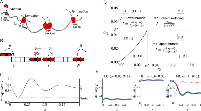
Figure 1: Illustration of the translation process, the inhomogeneous $\ell$-TASEP with open boundaries, and its phase diagram. A: Ribosomes initiate translation at the mRNA $5^{\prime}$ end, elongate the polypeptide by decoding one codon at a time, and eventually terminate the process by detaching from the transcript. B: Particles (of size $\ell=3$ here) enter the lattice at rate $\alpha$ and a particle at position $i$ (here defined by the position of the midpoint of the particle) moves one site to the right at rate $p_{i}$, provided that the move is not blocked by another particle in front. C: Example rate function with key parameters shown. D: The phase diagram is completely determined by $\lambda_{0},\lambda_{1},\lambda_{\min}$ and $\ell$. In this example, $(\lambda_{0},\lambda_{1},\lambda_{\min},\ell)=(0.9,0.3,0.1,10)$. All phase transitions are continuous in $J$ and, unless $\lambda_{\min}$ coincides with $\lambda_{0}$ or $\lambda_{1}$, discontinuous in $\rho$. E: Simulated results for $\ell=3,N=800$, and $\lambda$ as in C are compared with theoretical predictions. Dashed black and red lines represent upper and lower branches of solutions to (1). Circles are averaged counts over $5\times 10^{7}$ Monte-Carlo steps after $10^{7}$ burn-in cycles.

The hydrodynamic limit

The key quantities of interest are the stationary probability $\langle\tau_{i}\rangle$ of any individual site $i$ being occupied or not, and the current (or flux) $J$ of particles in the system. In the corresponding translation process, these quantities reflect the local ribosomal density and the protein production rate, respectively.

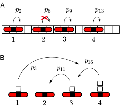
Figure S1: (Related to Figure 1A,B and The hydrodynamic limit of the inhomogeneous $\ell$-TASEP of STAR Methods). Correspondence between inhomogeneous $\ell$-TASEP (A) and the ZRP (B). $\ell$-TASEP particles (rods) correspond to ZRP sites, and holes (empty squares) become ZRP particles.

In the special case of the homogeneous $1$-TASEP ($p_{i}=p$ for all $i$ and $\ell=1$), the stationary distribution of the process decomposes into matrix product states, which can be treated analytically (Derrida et al.,, 1993). Unfortunately, in the general case this approach is intractable, necessitating alternative methods such as the hydrodynamic limit. When $\ell>1$, deriving the hydrodynamic limit is not straightforward, however, as the process does not possess stationary product measures (Schönherr and Schütz,, 2004). To tackle this problem, we mapped the $\ell$-TASEP to another interacting particle system called the zero range process (ZRP, see The hydrodynamic limit of the inhomogeneous $\ell$-TASEP of STAR Methods and Figure S1), whose hydrodynamic limit, assuming it exists, can be derived from the associated master equation. More precisely, we obtained the hydrodynamic limit through Eulerian scaling of time and space by a factor $a=N^{-1}$, and by following its dynamics on scale $x$ such that $k=\left\lfloor{\frac{x}{a}}\right\rfloor$, for $1<k<N$ (Rezakhanlou,, 1991). Implementing this limiting procedure for the ZRP and mapping it back to the inhomogeneous $\ell$-TASEP, we found that the limiting occupation density $\rho(x,t):=\mathbb{P}(\tau_{k}(t)=1)$, assuming its existence, satisfies the nonlinear PDE

$$\partial_{t}\rho=-\partial_{x}\left[\lambda(x)\rho\,G(\rho)\right]+\frac{a}{2}\partial_{xx}\left[\lambda(x)G(\rho)\right]+O(a^{2}),\hskip 8.53581pt$$ (1)

where $G(\rho)=\dfrac{1-\ell\rho}{1-(\ell-1)\rho}$ and $\lambda$ is a differentiable extension of $(p_{1},\ldots,p_{N})$, such that $\lambda(x)=\lambda(ka)=p_{k}$. More generally, this PDE takes the form of a conservation law with systematic and diffusive currents $J$ and $J_{D}$, given by

$$J(\rho,x)=\lambda(x)\rho G(\rho)\hskip 14.22636pt\text{and}\hskip 14.22636ptJ_{D}(\rho,x)=\dfrac{\lambda(x)\rho}{1-(\ell-1)\rho}.$$ (2)

As $a\ll 1$, the systematic current dominates and solutions of (1) generically converge locally uniformly on $(0,1)$ to so-called entropy solutions of

$$\partial_{t}\rho=-\partial_{x}\left[\lambda(x)\rho\,G(\rho)\right].$$ (3)

Further details and relevant calculations are provided in The hydrodynamic limit of the inhomogeneous $\ell$-TASEP of STAR Methods.

Particle densities, currents and phase transitions

The first order nonlinear PDE given by (3) can be solved using the method of characteristics (Evans,, 2010), which describes the evolution of differently dense “patches” of particles over time. Solving for the characteristics yields two branches of solutions, which we call “upper” and “lower” branches, while the boundary conditions imposed by $\alpha$ and $\beta$ determine which branch is taken by the stationary density of particles (see Phase transitions and profiles. of STAR Methods). As a consequence, the behavior of the system is characterized by a phase diagram in $\alpha$ and $\beta$. Moreover, this phase diagram depends on only few parameters of the system (see Figure 1C): the size of particles $\ell$, the jump rates at the boundaries, $\lambda_{0}:=\lambda(0)$ and $\lambda_{1}:=\lambda(1)$, and the minimum jump rate $\lambda_{\min}:=\min\{\lambda(x):x\in[0,1]\}$. In particular, these parameters determine the critical initiation and termination rates, $\alpha^{*}$ and $\beta^{*}$, that are associated with phase transitions. More precisely, the critical initiation rate $\alpha^{*}$ is given by

$$\alpha^{*}=\frac{\lambda_{0}-(\ell-1)J_{\max}}{2}\!\left[1-\sqrt{1-\dfrac{4\lambda_{0}J_{\max}}{\left[\lambda_{0}-(\ell-1)J_{\max}\right]^{2}}}\,\right],$$ (4)

where $J_{\max}=\frac{\lambda_{\min}}{(1+\sqrt{\ell})^{2}}$. Note that $\alpha^{*}$ is determined by the jump rates $\lambda_{0}$ and $\lambda_{\min}$. In the context of translation dynamics, this means that $\alpha^{*}$ will be specific to each gene, as different genes will likely have different values of $\lambda_{0}$ and $\lambda_{\min}$. For a fixed $\lambda_{0}$, the critical rate $\alpha^{*}$ increases as $\lambda_{\min}$ increases. For a fixed $\lambda_{\min}$, it turns out that $\alpha^{*}$ satisfies

$$\frac{\lambda_{\min}}{(1+\sqrt{\ell})^{2}}\leq\alpha^{*}\leq\frac{\lambda_{\min}}{1+\sqrt{\ell}},$$ (5)

where the lower bound is achieved as $\lambda_{0}\to\infty$, while the upper bound is achieved when $\lambda_{0}=\lambda_{\min}$. More generally, for a fixed $\lambda_{\min}$, the critical initiation rate $\alpha^{*}$ decreases as $\lambda_{0}$ increases. The critical termination rate $\beta^{*}$ is obtained from (4) by replacing $\lambda_{0}$ with $\lambda_{1}$. Hence, for mRNA translation, $\beta^{*}$ is also gene-specific, determined by the key elongation rates $\lambda_{1}$ and $\lambda_{\min}$.

The resulting phase diagram, which generalizes previous formulas for the homogeneous 1-TASEP (Derrida et al.,, 1993), is summarized as follows (see Figure 1D):

1. If $\alpha<\alpha^{\ast}$ and $\beta>\beta^{\ast}$ (LD I): In this regime the flux is limited by the initiation rate, leading to a low density profile. The corresponding current assumed by the system is

$$J_{L}=\frac{\alpha(\lambda_{0}-\alpha)}{\lambda_{0}+(\ell-1)\alpha},\\$$ (6)

while the site-specific particle density is

$$\rho_{L}(x)=\frac{1}{2\ell}+\frac{J_{L}(\ell-1)}{2\ell\lambda(x)}-\sqrt{\left[\frac{1}{2\ell}+\frac{J_{L}(\ell-1)}{2\ell\lambda(x)}\right]^{2}-\dfrac{J_{L}}{\ell\lambda(x)}}.$$ (7)

2. If $\alpha>\alpha^{\ast}$ and $\beta<\beta^{\ast}$ (HD I): Now the flux is limited by the particle exit rate, resulting in a high density regime. The associated current $J_{R}$ and density $\rho_{R}$ are identical to $J_{L}$ ((6)) and $\rho_{L}$ ((7)), respectively, with $\lambda_{0}$ and $\alpha$ replaced by $\lambda_{1}$ and $\beta$.

3. If $\alpha<\alpha^{\ast}$ and $\beta<\beta^{\ast}$ (LD II and HD II): The steady state is determined by the sign of $J_{L}-J_{R}$ (computed as above). If it is positive ($J_{L}>J_{R}$), the system is in a low density regime with current and density given by $J_{L}$ and $\rho_{L}$, respectively. Conversely, if it is negative, the system is in a high density regime with $J_{R}$ and $\rho_{R}$ as the current and density.

4. If $\alpha>\alpha^{\ast}$ and $\beta>\beta^{\ast}$ (MC): The system carries the maximum possible current (also referred to as the transport capacity of the system)

$$J_{\max}=\dfrac{\lambda_{\mathrm{min}}}{(1+\sqrt{\ell})^{2}},$$ (8)

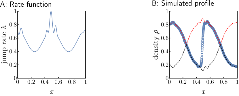
Figure S2: (Related to Particle densities, currents and phase transitions and Phase diagram analysis of STAR Methods). Atypical behaviour of MC branch switching in the presence of two global minima. Hydrodynamic predictions suggest that branch switching is bound to occur between any two global minima, but do not provide explicit information about the precise location of these singularities. Simulations indicate that branch switching is preferentially situated around local maxima. A: Elongation rates. B: Circles are averaged counts over $5\times 10^{7}$ Monte-Carlo steps after $10^{7}$ burn-in cycles on a lattice of size $N=2000$ with parameters $\alpha=\beta=\ell=1$ and elongation rate function shown in A. We compare these simulated densities to the theoretical profile obtained from the upper (red) and lower (black) branch solutions (described in (19)).

which is limited only by the minimum elongation rate $\lambda_{\min}$. Its density is characterized by qualitatively different profiles to the left and right of $x_{\mathrm{min}}=\arg\min_{x}\lambda(x)$: For $x<x_{\mathrm{min}}$, $\rho(x)$ is described by the upper branch (obtained by replacing $J_{R}$ with $J_{\max}$ in the equation for $\rho_{R}$), while for $x>x_{\mathrm{min}}$, $\rho(x)$ is described by the lower branch (obtained by replacing $J_{L}$ with $J_{\max}$ in $\rho_{L}$). That is, a branch switch occurs at $x_{\min}$ (where $\rho(x_{\min})=(1+\sqrt{\ell})^{-2}$). We proved more generally that every global minimum of $\lambda$ regulates the traffic of particles (like a toll reducing the traffic flow) in this fashion: incoming densities to the left of it are always described by the upper branch whereas outgoing particles on the right follow the lower branch. In particular, this implies that in the case of multiple global minima, the density between two consecutive minima must undergo a discontinuous jump from lower to upper branch (for more details, see Phase transitions and profiles. of STAR Methods and Figure S2).

Novel phenomena and applicability to discrete lattices

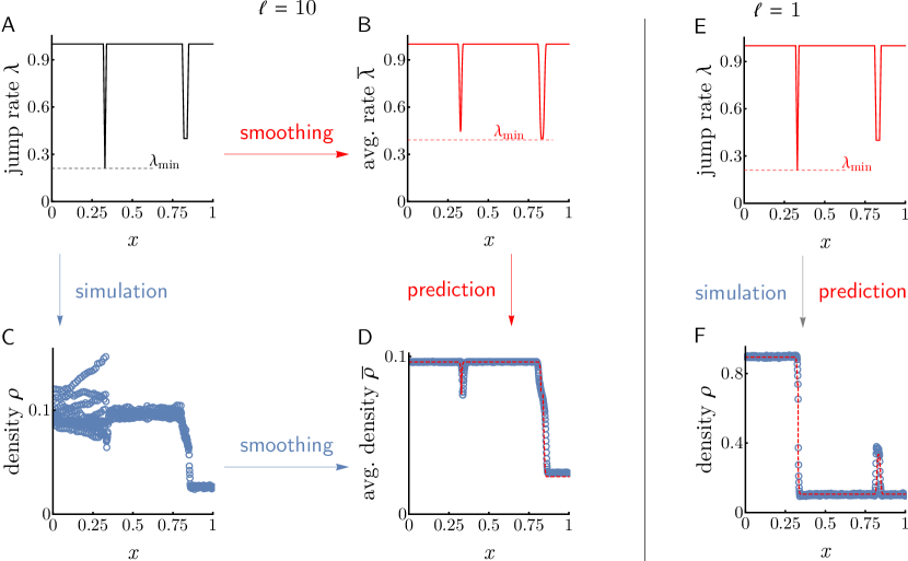
Figure S3: (Related to Figure 2 and Phase transitions and profiles. of STAR Methods). MC branch switching is determined by locally averaged elongation rates rather than raw elongation rates (A-D), and the averaging scale depends on the particle size (E,F). Both the value as well as the location of the minimal elongation rate may differ significantly when measured with respect to the discrete elongation profile (Panel A) or smoothed elongation profile (Panel B). Panels C and D demonstrate that our hydrodynamic prediction is very accurate, and show that MC branch switching is governed by the smoothed elongation profile rather than its discrete counterpart. Several of the yeast transcripts we analyzed are affected by this phenomenon, suggesting that a codon’s local neighborhood is a stronger determinant of translation dynamics than the absolute elongation rate at that site. Whether smoothed elongation rates (as opposed to unsmoothed rates) describe the translation dynamics more accurately is strongly linked to the particle size $(\ell)$ and the long-range correlations (in particular, $\ell$-periodicity after traffic jams) it induces. To demonstrate this point, we performed the same analysis as in Panels A-D using particles of size $\ell=1$. We found that our hydrodynamic predictions based on the raw, unsmoothed elongation rates (Panel E) does indeed provide an accurate approximation of simulated densities (Panel F). In short, the fact that the ribosome occupies 10 codons (i.e. the “particle” size is $\ell=10$) provides another reason (in addition to alleviating the irregularity of elongation rates that cause analytical difficulty) for why smoothing the elongation rates is the right thing to do when applying the hydrodynamic limit of the $\ell$-TASEP to study mRNA translation.

As shown in Figure 1E, for smooth rate functions the densities predicted by our analysis agree well with Monte Carlo simulations in all regimes of the phase diagram. In the context of translation dynamics, however, elongation rates are typically less regular, exhibiting substantial fluctuations throughout the entire transcript (see Figure 2A). Despite this lack of regularity, the hydrodynamic limit can still be employed to describe local averages of such a system. In particular, smoothing particle profiles by windows of length $\ell$ reproduces parameters that closely match hydrodynamic predictions (see Applicability to discrete lattices of STAR Methods and Figure S3). Hence, all subsequent analyses described below will pertain to elongation rate profiles smoothed by a ten-codon moving average. A noteworthy consequence of the above results is that local averages of elongation rates are more predictive of overall translation dynamics than their non-smoothed counterparts. In particular, the location at which branch switching occurs in the MC regime is governed by $x_{\min}=\arg\min_{x}\{\overline{p}_{x}\}/N$ which may be, and in many cases is, considerably different from $\arg\min_{x}\{p_{x}\}/N$ (cf. Figure S3).

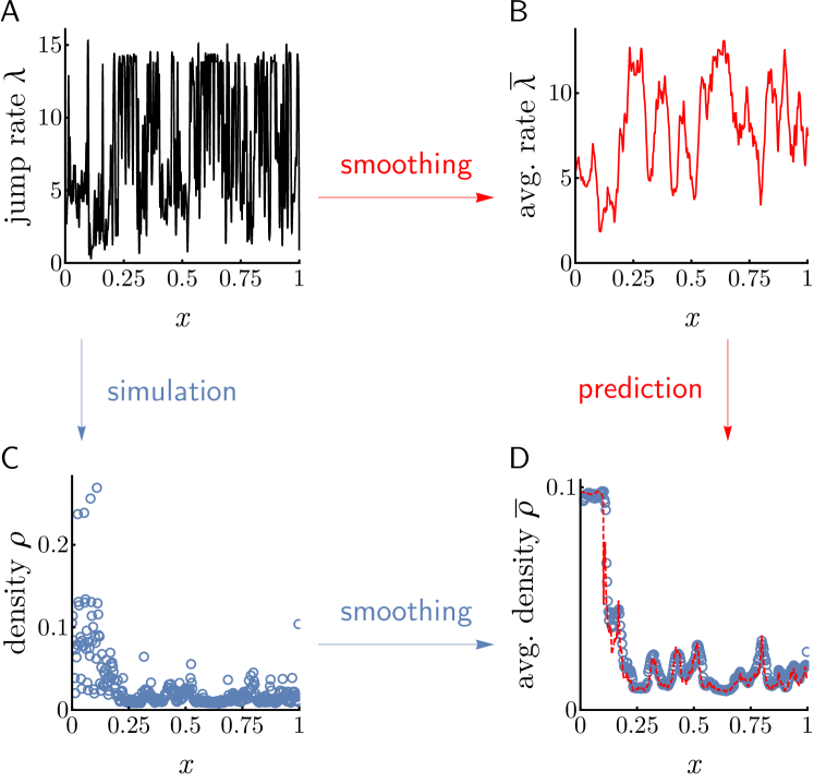
Figure 2: Local averaging reproduces hydrodynamic limit in lattices with discontinuous rate functions. Applying the hydrodynamic theory to smoothed jump rates correctly predicts smoothed density profiles and currents. A: Elongation rates of the yeast gene YHR025W arbitrarily chosen from Dao Duc and Song, (2018) (see Empirical Study: Translational Efficiency in Yeast for further details). B: Smoothed elongation rates obtained by applying a ten-codon moving average to the raw profile in A. C: Density profile resulting from simulation (as in Figure 1E except with $\ell=10,N=357$) under discontinuous profile in A. D: The hydrodynamic density profile (dashed red) associated with the smoothed elongation rates of B reproduces the smoothed density profile obtained from averaging the raw densities in C by a moving ten-codon window. Similarly, simulated and predicted currents are in excellent agreement ($0.1072$ and $0.1077$, respectively).

We highlight a few novel phenomena in our generalization of the homogeneous $1$-TASEP: First, extending particles to size $\ell>1$ and lowering the limiting jump rate $\lambda_{\min}$ reduces both the transport capacity $J_{\max}$ and the critical rates ($\alpha^{*}$ and $\beta^{*}$) for entrance and exit, leading to an enlarged MC phase region. This is expected as fewer particles are needed to saturate the lattice, and distances between particles are larger, which in turn limits the number of particles able to cross a site per given time. This phenomenon is quantified precisely using our explicit expressions for $\alpha^{\ast},\beta^{\ast}$, and $J_{\max}$ (see (4) and (8)). Second, the inhomogeneity in $\lambda$ may deform the LD-HD phase separation from being a straight line in the homogeneous $\ell$-TASEP (Chou and Lakatos,, 2004) to a generally nonlinear curve (see Figure 1D) determined by solutions $(\alpha,\beta)$ of

$$\frac{\alpha(\lambda_{0}-\alpha)}{\lambda_{0}+(\ell-1)\alpha}=\frac{\beta(\lambda_{1}-\beta)}{\lambda_{1}+(\ell-1)\beta},$$ (9)

corresponding to the condition $J_{L}=J_{R}$. This is a consequence of $\alpha$ and $\beta$ affecting the system at different scales whenever $\lambda_{0}\neq\lambda_{1}$, resulting in a phase diagram that is no longer symmetric. Lastly, our observation of density profiles performing branch switching in the MC phase was indiscernible in the homogeneous case, as the high density and low density branches merge into a single value (viz. $\rho=\frac{1}{\sqrt{\ell}+\ell}$).

Application: Design Principles for Translational Systems

We sought to apply our theoretical analysis to understand how the translational system can be regulated and optimized with regard to protein synthesis rate and ribosome usage. The hydrodynamic theory developed above singles out the key parameters that determine the current and particle densities. We illustrate in Figure 3 how $\lambda_{0}$, $\lambda_{\min}$, and $x_{\min}$ impact the current capacity, its sensitivity to the initiation rate $\alpha$, and the global particle density, suggesting the following principles:

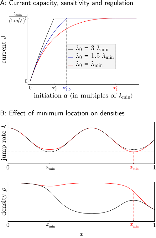
Figure 3: Main determinants of current and particle densities. A: We plot the current $J$ in LD and MC against the initiation rate $\alpha$, for various choices of $\lambda_{0}$. While $\lambda_{\min}$ governs the maximum current at which $J$ reaches a plateau (coinciding with the transition from LD to MC), changing the size of $\lambda_{0}$ results in changes in $\partial_{\alpha}J$, the sensitivity of $J$ with respect to $\alpha$. Distinct configurations of $\lambda_{\min}$ and $\lambda_{0}$ give rise to vastly different dependencies of $J$ on $\alpha$, suggesting different responses to global changes in the ribosome pool. $\alpha^{*}_{3}$, $\alpha^{*}_{1.5}$, and $\alpha^{*}_{1}$ correspond to the $\alpha^{*}$ value (in units of $\lambda_{\min}$) when $\lambda_{0}=3\lambda_{\min},\lambda_{0}=1.5\lambda_{\min},$ and $\lambda_{0}=\lambda_{\min}$, respectively. B: Two elongation rate profiles that differ slightly in overall shape, but drastically in their position $x_{\min}$ of minimum elongation are plotted (top panel) together with their associated MC ribosome densities (bottom panel). The branch switching phenomenon has extreme consequences for equilibrium particle densities and hence ribosomal costs, with elongation rate profiles achieving minimum rates close to the initiation site (top, dotted black curve) benefiting from drastic savings (bottom, black curve) compared to otherwise similar profiles (red curves).

1. The initiation rate $\alpha$ (and not termination rate $\beta$) should regulate the production rate $J$. As shown by our analysis of the current, any value of the current that lies below the system’s production capacity $J_{\max}$ can be attained through either HD or LD regime. In order to avoid overuse of resources, however, a transcript should always operate in LD, where the main determinant for currents is the initiation rate $\alpha$ (cf. (6)). To guarantee LD profiles, termination rates merely need to exceed the critical value $\beta^{\ast}$, whereas initiation rates are more tightly controlled, varying between $0$ and $\alpha^{\ast}$. Within this interval, the current $J$ increases with $\alpha$ according to (6), as illustrated in Figure 3A.

2. The minimum elongation rate $\lambda_{\min}$ determines the production capacity $J_{\max}$. As $\alpha$ increases in the LD regime, the current $J$ reaches a plateau that is associated with the maximal current (MC) regime (see Figure 3A). By (8), the maximum possible current is directly proportional to $\lambda_{\min}$, which therefore sets the range within which production rates may vary. Large values of $\lambda_{\min}$ allow for both constitutively high expression of genes as well as highly variable protein levels, while small values of $\lambda_{\min}$ guarantee constitutively low expression.

3. In the LD regime, the sensitivity of production rate $J$ to $\alpha$ is moderated by $\lambda_{0}$ and varies across different values of $\alpha$. Our theory predicts that for $\beta>\beta^{*}$ (i.e., provided that the termination rate is sufficiently high), the dynamic range of the initiation rate (i.e., the range of $\alpha$ within which the overall protein production rate $J$ varies with $\alpha$) is given by $(0,\alpha^{*})$, where the critical initiation rate $\alpha^{*}$ is defined in (4). Furthermore, the degree to which $J$ varies with $\alpha$ is fully determined by the elongation rate $\lambda_{0}$, as shown in (6). Indeed, $\lambda_{0}$ controls the time spent by particles at the start of the lattice, and can induce significant buffering if $\alpha$ is large enough, thereby modulating the effective rate of entrance associated with $J$. We illustrate this in Figure 3A, where we compare how the current varies as a function of $\alpha$ for different values of $\lambda_{0}$ relative to $\lambda_{\min}$. Recall that the critical initiation rate $\alpha^{*}$ satisfies the inequalities in (5), and that $\alpha^{*}$ increases as $\lambda_{0}$ decreases. Figure 3A also shows that for $\lambda_{0}$ fixed, the production rate of a system closer to the MC regime (i.e., with $\alpha$ just below $\alpha^{*}$) is less sensitive to changes in $\alpha$, and that this effect is more pronounced the closer $\lambda_{0}$ is to $\lambda_{\min}$. More generally, the $\alpha$-sensitivity of $J$ increases as $\lambda_{0}$ increases. While the dependence of $J$ in $\alpha$ is sublinear for $\lambda_{0}=\lambda_{\min}$, it becomes linear as $\lambda_{0}$ gets large (see (6)). This suggests in particular that changes in the free ribosome pool (changing the initiation rate globally) can impact the protein production rate differently across different genes.

4. Positioning $\lambda_{\min}$ close to the start site can reduce the amount of ribosomes used. At maximum production capacity (MC regime), we have shown that the density profile follows the high density branch from the start of the lattice until the location $x_{\min}$ of $\lambda_{\min}$ whereafter it adopts the low density branch. This characteristic branch switching phenomenon makes $x_{\min}$ critical for the purpose of resource allocation. In Figure 3B, we illustrate how a small local change in the rate function can induce a large increase of average particle density when $x_{\min}$ changes substantially. Therefore, a way to limit the excessive usage of ribosomes induced by traffic jams at maximum capacity is to position the minimum rate close to the start. However, as previously shown, positioning it too close to the start (such that $\lambda_{0}=\lambda_{\min}$) would also decrease the sensitivity of the system to $\alpha$.

Empirical Study: Translational Efficiency in Yeast

In light of the aforementioned principles, we explored the extent to which the translational system in yeast is efficient. For this study, we used elongation rates previously inferred from ribosome profiling data for a set of 850 genes in S. cerevisiae (Dao Duc and Song,, 2018) (see Data processing of STAR Methods). These genes were selected in Dao Duc and Song, (2018) based on length and footprint coverage, to yield robust estimates of rates. The advantage of using this particular dataset over most others lies in the fact that the inferred rates for this subset of genes faithfully reproduce ribosome profiling data, incorporating several experimental artifacts of ribo-seq such as undetected stacked ribosomes, thereby minimizing confounding from technical biases. Furthermore, primarily analyzing high-coverage (and thus likely highly expressed) genes does not confound our study of design principles, but rather provides us an increased signal-to-noise ratio, as these genes are precisely those on which our design principles are expected to act most strongly.

We analyzed the location of these 850 genes in the phase diagram, and the distribution of the key parameters and variables that determine the ribosomal currents and densities. We found the aforementioned theoretical design principles being reflected as follows:

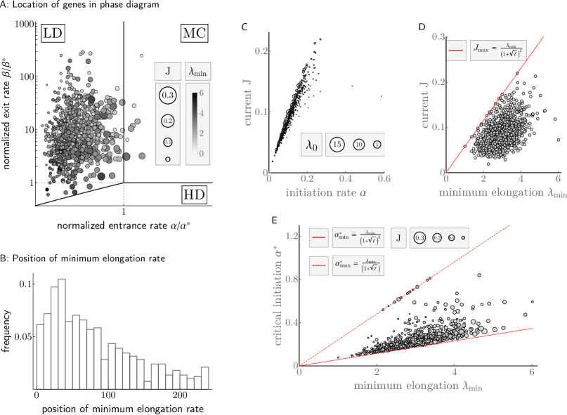
Figure 4: Translation machinery in S. cerevisiae optimizes for ribosomal cost, flexible regulation and production capacity. All rates are in codons per second, while currents are measured in ribosomes per second. A: 850 genes of S. cerevisiae are located in the phase diagram, with size and hue of each data point reflecting current and minimum elongation rate, respectively. On a population level, systems of comparable production capacities ($\propto\lambda_{\min}$) fully exploit their dynamic range by adjustment of $\alpha$, with highly expressed proteins likely situated inside or close to MC. B: The resulting resource cost considerations drive a significant number of transcripts to position their minimum elongation rate early on in the codon sequence, forcing ribosomal traffic jams to remain short. C: Initiation $\alpha$ is the main determinant of currents, at least for low to average current genes. For highly expressed genes, the correlation between $\alpha$ and $J$ decreases due to stronger variation in $\lambda_{0}$ and transitions into MC. D: Genes utilize the full dynamical range of currents set by $\lambda_{\min}$, through variation in $\alpha$ and $\lambda_{0}$. Constitutively highly expressed genes tend to be closer to maximum capacity (red line), while genes with variable expression demands are distributed more broadly (see main manuscript). E: For fixed production capacity $\propto\lambda_{\min}$, $\alpha^{\ast}$ (the critical initiation rate at which genes reach maximum production capacity) tends to be smaller for genes with larger production rates. That is, larger $\lambda_{0}$ (which are inversely related to $\alpha^{\ast}$ for fixed $\lambda_{\min}$) seem to facilitate attainment of large currents. Moreover, within highly expressed genes, those associated with variable expression patterns over time exhibit higher sensitivities (smaller $\alpha^{\ast}$), whereas genes with constitutive high expression are found closer towards maximal insensitivity (dotted red line) as these configurations ease stable expression.

1. Translation mainly operates in LD regime. Upon computing $\alpha^{*}$ and $\beta^{*}$, we located the position of each gene in the phase diagram (see Figure 4A). Over the 850 genes in our dataset, we found 841 in LD and the remaining 9 in the MC region. No genes were found in HD, suggesting no excessive usage of ribosome to achieve any protein level. As a result, the initiation rate is the main determinant and limiting factor of the current (Spearman’s rank correlation coefficient $\rho=0.979$). The strength of this correlation nevertheless decreases as genes get closer to the MC regime, since $J$ becomes less sensitive to $\alpha$ and $\lambda_{\min}$ becomes its rate limiting factor (see Figure 4C). To quantify this reduction in correlation, we binned the data by quartiles of $J$ and computed Spearman correlations within each bin, which yielded (in order of quartiles): $0.93,0.72,0.64,$ and $0.58$.

2. Wide ranges of currents are covered within production capacity. For each gene in our dataset, we examined the maximal protein production rate, which according to our theory is proportional to $\lambda_{\min}$. The data exhibit an overall range of $\lambda_{\min}$ between $1.01$ and $6.01$ codons/second, and for any fixed $\lambda_{\min}$, currents are well spread out across $[0,J_{\max}]$ (see Figure 4D). Given that genes cover almost all of the theoretically possible range of currents, we investigated whether certain configurations of $\lambda_{\min}$ and $J$ are associated with the biological function of specific genes. To do so, we compared ribosomal protein genes (known to be highly expressed) and genes related to stress response (requiring variable expression over time, see Data processing of STAR Methods). We found that, while both sets of genes display comparable $\lambda_{\min}$, ribosomal genes are more likely to be close to their maximal production capacity ($p<7\times 10^{-3}$, see QUANTIFICATION AND STATISTICAL ANALYSIS of STAR Methods) and more consistently so (the coefficient of variation is 0.22 for ribosomal genes and 0.36 for stress response).

3. $\lambda_{0}$ (associated with sensitivity to $\alpha$) is higher for genes that are either highly expressed or subject to varying expression demand. The impact of increasing $\alpha$-sensitivity is primarily twofold: First, for fixed production capacity, large currents may be attained with smaller initiation rates; and second, more substantial changes in currents may be achieved with small changes in $\alpha$. To investigate the former we computed $\alpha^{\ast}$, the critical rate necessary for a gene to attain maximum capacity, across all genes whose $\lambda_{\min}$ exceeded the median $\lambda_{\min}$ of the data set (as large currents presuppose large capacities). Further binning this range into quartiles (to isolate the dependence of $\alpha^{\ast}$ on $\lambda_{0}$), we found that genes whose currents are at least $90\%$ of the production capacity are significantly more sensitive ($p<0.008,0.01,0.05,$ and $0.004$, respectively; see Figure 4E), requiring smaller initiation rates to reach peak production rate (cf. Figure 4C). To inspect the second aspect of $\lambda_{0}$ as facilitator or inhibitor of rapid changes in current, we explored the ratio of $\lambda_{0}$ to $\lambda_{\min}$ again in ribosomal and stress response genes. For constitutively highly expressed genes like ribosomal genes, we expect this ratio to be small to maintain stable current close to MC (cf. Figure 3), whereas genes with variable expression demands like the ones associated with stress response should exhibit larger ratios. Confirming this intuition, we found significantly reduced levels of $\lambda_{0}/\lambda_{\min}$ in ribosomal genes ($p<2\times 10^{-6}$), and significantly increased levels in stress response genes ($p<0.04$).

4. The position of $\lambda_{\min}$ is preferentially located early in the open reading frame. Upon analyzing the distribution of $x_{\min}$ from our dataset (see Figure 4B), we found it preferentially located in the codon positions between 30 to 40, consistent with genes forestalling excessive ribosome usage through enforcing branch switching early on. More specifically, we reasoned that both genes closer to MC and those highly sensitive to $\alpha$ run higher risk of incurring substantial ribosome cost and should thus locate $x_{\min}$ early in the coding sequence. Indeed, both the top quartile of genes close to MC (as measured by $\alpha/\alpha^{\ast}$) and stress response associated genes showed significantly smaller $x_{\min}$ ($p<0.03$ and $0.01$, respectively). Moreover, genes with unusually large values of $x_{\min}$ are significantly less likely to be close to MC (top quartile of $x_{\min}$: $p<1\times 10^{-3}$).

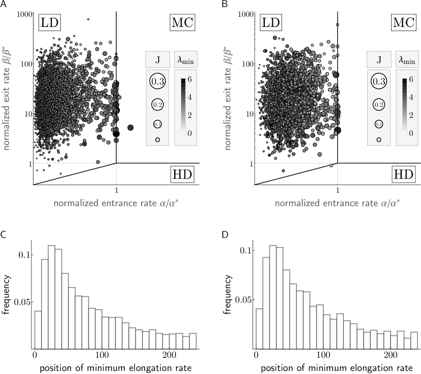
Figure S4: (Related to Empirical Study: Translational Efficiency in Yeast and Figure 4). Inferences on the efficiency of yeast’s translational system are consistent across datasets. To test the replicability of our analysis using the previously inferred elongation rates in Dao Duc and Song, (2018) and to exclude any possible systematic biases, we repeated our inference on elongation rates obtained by inverting (3) on two independent ribosome profiling datasets: One compiled by Williams et al., (2014) (A, C, total of $3098$ genes), and one by Pop et al., (2014) (B, D, total of $2536$ genes). The clear localization of genes within LD and at the LD/MC boundary, together with a characteristic ramp-shaped distribution of the minimum elongation location remain apparent, lending support to our proposed design principles holding true not only on the 850 genes analyzed in the main manuscript, but more generally as a framework governing translation efficiency.

To check for systematic biases potentially present in our subsampled gene set and to show replicability of our main biological conclusions, we also analyzed two other independent (and much larger) datasets from Williams et al., (2014) (combined with polysome profiling from MacKay et al., (2004)) and Pop et al., (2014) (see Data Processing of STAR Methods). We inverted the solution of (3) to obtain approximate estimates of initiation rates, termination rates, and smoothed elongation rates for these datasets, and repeated our analyses. As shown in Figure S4, the results are generally in excellent agreement with what is discussed above (Figure 4A,B).

DISCUSSION

While past quantitative studies of the TASEP under general conditions of extended particle size and/or rate heterogeneity have mostly been limited to numerical simulations or mean-field approximations, (Lakatos and Chou,, 2003; Shaw et al.,, 2003, 2004; Chou and Lakatos,, 2004; Dong et al.,, 2007), we used here a different approach that relies on studying the hydrodynamic limit of the process. In the case of homogeneous rates, previous studies (Schönherr,, 2005; Schönherr and Schütz,, 2004) established this hydrodynamic limit, but without further analyzing the subsequent PDE. After deriving this limit for inhomogeneous rates, we obtained closed-form formulas for the associated current, densities, and phase diagram, generalizing previous theoretical results for the TASEP (Derrida et al.,, 1993; Blythe and Evans,, 2007) and its variants (Shaw et al.,, 2003; Chou and Lakatos,, 2004; Stinchcombe and de Queiroz,, 2011). Our approach has the advantage of revealing the key parameters that the current and densities depend on, enabling an immediate quantification of the process and its phase diagram. Such a quantification is difficult to achieve via conventional stochastic simulations or approximations used in the past several years (Zia et al.,, 2011; Zur and Tuller,, 2016; Szavits-Nossan et al.,, 2018).

Our characterization of the current and densities in the phase diagram suggests that, in agreement with earlier experimental studies (Kosuri et al.,, 2013; Salis et al.,, 2009), translation dynamics should be mainly governed by the initiation rate, while the termination rate and most elongation rates have negligible impact. In particular, our results explain why having the initiation rate as the main limiting factor of the current (Plotkin and Kudla,, 2011) minimizes ribosome usage. In addition, we discovered the importance of smoothed rather than raw elongation profiles in predicting translation dynamics, explaining the previously observed mild effect that any individual elongation change has compared to accumulated, neighboring changes (Levin and Tuller,, 2018). This allowed us to identify two key parameters of the system, namely, the smoothed elongation rate $\lambda_{0}$ immediately following initiation and the minimal smoothed elongation rate $\lambda_{\min}$. Previous studies have established some association between the sequence context in the early $5^{\prime}$ coding region and protein production levels (Frumkin et al.,, 2017; Boël et al.,, 2016; Ben-Yehezkel et al.,, 2015). For example, it has been shown that mRNA secondary structure in the first $\sim 16$ codons (which locally decreases the elongation rate) negatively affects the translation rate in E. Coli, while no significant contribution of mRNA folding in other regions was found (Frumkin et al.,, 2017). By exposing $\alpha$ and $\lambda_{0}$ as the only parameters that currents in LD depend on, our analysis suggests a direct explanation for such contrast.

We also highlighted the impact of $\lambda_{0}$ on the sensitivity of the current to changes in $\alpha$. In practice, initiation rates can vary at the individual gene level (e.g., through interactions with specific miRNAs (Humphreys et al.,, 2005)). According to our theory, the way that these variations impact the protein production rate depends on $\lambda_{0}$; we hence suggest that this may explain why genes associated with stress response present higher values of $\lambda_{0}$, as it facilitates the response to changes in $\alpha$. At a more global level, our study shows how protein levels can be more or less robust against changes in the ribosomal pool, which can simultaneously affect all initiation rates in a cell (Shah et al.,, 2013). Since the level of ribosomes present in a cell fluctuates over time (Wyant et al.,, 2018), it would be interesting to see if protein levels scale uniformly with these variations across genes, and if not, whether the differences in $\lambda_{0}$ can explain it.

To the best of our knowledge, the role of the minimum elongation rate $\lambda_{\min}$ has so far received attention only indirectly, through the study of what is known as the “$5^{\prime}$ translational ramp” (Tuller et al.,, 2010). This ramp is a pattern of translational slowdown around codon position $30$-$50$ followed by steadily accelerating elongation rates, which is mirrored by the spatial distribution of minimum elongation rates we found here. This ramp has been hypothesized to prevent crowding of ribosomes on the transcript (Tuller et al.,, 2010), for which we provide a theoretical basis, exposing $\lambda_{\min}$ as a separator between crowded and freely elongating ribosomes. More generally, the complex interplay between the maximum current capacity, ribosome usage, and sensitivity to the initiation rate suggests various ways to set the parameters $\lambda_{0}$, $\lambda_{\min}$ and $x_{\min}$, depending on the desired object to optimize. For example, allocating the minimum elongation rate near the beginning of the ramp region provides an optimal trade-off between high sensitivity and minimal traffic jams. On the other hand, it would be optimal for genes with housekeeping function to have a decreased sensitivity, which would push the minimum to earlier positions.

Our analysis can also help to answer the long-debated question regarding the implication of translation on codon usage bias (Hershberg and Petrov,, 2008; Frumkin et al.,, 2018; Shah et al.,, 2013). Since highly expressed genes are enriched for synonymous codons translated by more abundant tRNAs (Yu et al.,, 2015; Hanson and Coller,, 2018), it has been hypothesized that codon usage bias increases the overall protein synthesis rate by accelerating elongation (Hershberg and Petrov,, 2008). However, recent studies have challenged such a hypothesis, suggesting that translational selection for speed is not sufficient to explain the observed variation in codon usage bias (Mahajan and Agashe,, 2018). Synonymous changes of the coding sequence modify local elongation rates, but, according to our theory, such a modification impact the overall protein production rate only if the smoothed elongation rates $\lambda_{0}$ or $\lambda_{\min}$ are affected. In addition, our work implies that synonymous codon replacements that substantially change the location $x_{\min}$ of $\lambda_{\min}$ affect the efficiency of ribosome usage, and hence are more likely to be under selective pressure. Aside from these cases, there should be little direct impact of synonymous codon usage on translation efficiency; this prediction is consistent with previous studies that tried to explain differences in expression using codon identity (Gustafsson et al.,, 2012), and to characterize the sensitivity of translational output with respect to changes in elongation (Levin and Tuller,, 2018). Codon usage bias could affect the protein production rate indirectly, however, by reducing the cost of translation: replacing a codon by a “faster” synonymous codon helps to reduce the local ribosome density on the transcript, and this can in turn increase the availability of free ribosomes and therefore increase the initiation rate $\alpha$ slightly; in the LD regime, increasing $\alpha$ would increase the protein production rate. We note that other factors such as mRNA decay (Hanson and Coller,, 2018), or reduction of nonsense errors or co-translational misfolding (Gilchrist,, 2007; Frumkin et al.,, 2018) might be more important drivers of codon usage bias.

Finally, it would be interesting to experimentally test our theoretical predictions, e.g., using cell-free expression protocols such as lysate-based systems, which have been developed to optimize protein synthesis and more recently refined to study translation dynamics (Moore et al.,, 2017; Rosenblum and Cooperman,, 2014; Katranidis and Fitter,, 2019). By designing an appropriate mRNA sequence and controlling different components (NTPs, ribosomes, tRNAs, specific amino acids), these systems allow to manipulate the initiation and elongation rates, and hence tune the key parameters identified by our theoretical analysis. For example, one can modify $\lambda_{\min}$ or $\lambda_{0}$ by changing the level of corresponding amino acids, and vary $\alpha$ by modifying the $5^{\prime}$ UTR sequence or changing the ribosome concentration. The flexible nature of such cell-free expression systems, coupled with precise measurement of protein levels (e.g., via isotope-labeled amino acids or reporter proteins), should help to verify our theoretical results. In particular, it would be interesting to experimentally demonstrate the existence of phase transitions, and by modifying the mRNA sequence, test our predictions on how to effectively control the robustness and sensitivity of the translation system. We are currently pursuing these research directions.

DECLARATION OF INTERESTS

The authors declare no competing interests.

STAR METHODS

LEAD CONTACT AND MATERIALS AVAILABILITY

Further information and requests for resources and reagents should be directed to and will be fulfilled by the Lead Contact, Yun S. Song (yss@berkeley.edu).
This study did not generate new reagents.

METHOD DETAILS

The hydrodynamic limit of the inhomogeneous $\ell$-TASEP

We derive here the PDE governing the hydrodynamic limit of the open-boundaries inhomogeneous $\ell$-TASEP. To do so we exploit a representation of its dynamics in terms of another interacting particle system, the so-called zero range process (ZRP), whose hydrodynamics can be found explicitly. This TASEP-ZRP duality provides an expedient and general tool for identifying explicit TASEP formulas; however, rigorously proving the validity of these formulas often requires more technical tools from probability theory. Since this work’s emphasis is on the application of TASEP to unraveling the key parameters of translation dynamics, we will here concentrate on showcasing the TASEP-ZRP framework, and keep a rigorous existence proof of the hydrodynamic limit, combining techniques from Rezakhanlou, (1991); Covert and Rezakhanlou, (1997) and Bahadoran, (2012), to a separate manuscript.

Reduction to periodic boundaries and mapping to the ZRP.

The purpose of the hydrodynamic limit is to describe the local evolution of the macroscopic particle density in the large system limit. As such, it does not explicitly rely on the precise formalism by which particles enter and exit the lattice at the boundaries (which will only later be needed to impose boundary conditions on the resulting PDE (Bahadoran,, 2012)). In particular, we are free to choose periodic boundary conditions for our limiting procedure without changing the resulting PDE (Schönherr and Schütz,, 2004). This has the advantage of preserving the total number of particles, which is essential for establishing the correspondence between TASEP and ZRP. In the following, we thus consider the $\ell$-TASEP with $M$ particles on a ring of $N$ sites jumping to the right at rate $p_{i}$, and take $M,N\to\infty$ while $M/N$ remains constant.

The ZRP is now obtained by reversing the roles of holes and particles: It consists of $N-M\ell$ particles (corresponding to the $N-M\ell$ holes in the TASEP) distributed across $M$ sites (matching the TASEP particles) $\{1,\ldots,M\}$, with multiple particles allowed to stack up on the same site. A ZRP configuration $(\xi_{i,t})_{1\leq i\leq M}$ describes the number of particles $\xi_{i,t}$ at each site $i\in\{1,\ldots,M\}$ and time $t$, and can be seen as a representation of spacings between particles $i$ and $i+1$ in the TASEP.

As a result, the TASEP dynamics are translated into ZRP dynamics as follows: If a site $i$ at time $t$ is occupied by at least one particle, then the topmost particle jumps to the left with rate $m_{i,t}=p_{k(i,t)}$, where $k(i,t)$ is the position of the $i$th TASEP particle (see formula (10) below) at time $t$. This jump occurs regardless of whether the destination site is occupied or not. That is, neither exclusion nor long range interactions are present, which will be key to establishing the hydrodynamic limit.

The correspondence between TASEP and ZRP states described above is so far only determined up to rotations of the TASEP lattice, hence we introduce one further variable $\xi_{0,t}\in\{1,\ldots,N\}$ to trace the position of particle $1$. More explicitly, at time $t$, TASEP particle $i$ is located at site

$$k(i,t)=\sum_{j=0}^{i-1}\xi_{j,t}+\ell(i-1)$$ (10)

on the TASEP ring. An illustration of this correspondence is given in Figure S1.

The hydrodynamic limits of the ZRP and TASEP.

The connection between the TASEP and the ZRP has been fruitfully used to derive hydrodynamic limits for homogeneous systems (Schönherr and Schütz,, 2004; Schönherr,, 2005). Here we generalize this approach to heterogeneous lattices and supply appropriate boundary conditions to the PDE, which become necessary when working with open rather than periodic boundaries.

We start with the master equation associated with the ZRP:

$$\partial_{t}\xi_{i,t}=m_{i+1,t}z_{i+1,t}-m_{i,t}z_{i,t},$$ (11)

where $z_{i,t}=\mathbb{P}(\xi_{i,t}>0)$ is the probability that site $i$ is non-empty at time $t$. Our goal is to identify a PDE that describes the limit of (11) under Euler scaling, i.e., on time scale $at$ and spatial scale $ia$. Denoting these scaled variables as $t$ again in time and $x,y$ in space such that $k=\lfloor x/a\rfloor$ and $i=\lfloor y/a\rfloor$, and assuming the existence of a continuously differentiable rate function $\lambda$ such that $\lambda(x)=p_{k}$, the master equation (11) becomes

$$a\partial_{t}c(y,t) =\lambda(x(y+a,t))z(y+a,t)-\lambda(x(y,t))z(y,t)$$

$$=a\partial_{y}[\lambda(x(y,t))z(y,t)]+\dfrac{a^{2}}{2}\partial_{yy}[\lambda(x(y,t))z(y,t)]+O(a^{3}),$$ (12)

where $c(y,t)$ and $z(y,t)$ are the continuum limits of $\xi_{i,t}$ and $z_{i,t}$, respectively. Under local stationarity (Kipnis and Landim,, 2013), we may replace $z$ in (12) using the fugacity-density relation $z=c(1+c)^{-1}$ to obtain the final hydrodynamic limit of the inhomogeneous ZRP as

$$\partial_{t}c=\partial_{y}\bigg{(}\lambda\dfrac{c}{1+c}\bigg{)}+\dfrac{a}{2}\partial_{yy}\bigg{(}\lambda\dfrac{c}{1+c}\bigg{)}.$$ (13)

The assumption of local stationarity is essentially justified by the one-block estimates in Covert and Rezakhanlou, (1997), as long as one can ensure slow enough variation of $\lambda(x(y,t))$ in $t$. In our case, this smooth dependency is given, since in a small (on the Eulerian scale) time interval $N\Delta t$, we expect a particle to perform $O(N\Delta t)$ jumps, and whence $\lambda(x(y,t+N\Delta t))-\lambda(x(y,t))\in O(\Delta t)$.

To derive the corresponding PDE for the TASEP, we use (10) to establish the continuum relation between $x,y$ and $t$. More precisely,

$$x(y,t)=ak(i,t)=a\bigg{(}\sum_{j=0}^{i-1}\xi_{j,t}+\ell(i-1)\bigg{)}=\int_{0}^{y}c(u,t)\ \mathrm{d}u-\dfrac{a}{2}\bigg{(}c(y,t)-c(0,t)\bigg{)}+\ell(y-a)+O(a^{2}).$$ (14)

Upon recognizing that particle densities are related by $\rho=(c+\ell)^{-1}$ and changing coordinates according to (14), (13) yields the hydrodynamic limit of the TASEP

$$\partial_{t}\rho=-\partial_{x}\left[\lambda(x)\rho G(\rho)\right]-\frac{a}{2}\partial_{xx}\left[\lambda(x)G(\rho)\right]+O(a^{2}),$$ (15)

where $G(\rho)=\frac{1-\ell\rho}{1-(\ell-1)\rho}$.

Phase diagram analysis

We now use (15) to provide a detailed derivation of the phase diagram described in the main text.

Reduction to conservation law.

Solutions of (15) converge locally uniformly (under mild conditions on $\lambda$, see Phase transitions and profiles.) to viscosity solutions of the scalar conservation law

$$\partial_{t}\rho(x,t) =-\partial_{x}[\underbrace{\lambda(x)H(\rho(x,t))}_{J(\rho(x,t),x)}],$$ (16)

where $H(\rho)=\rho G(\rho)$, which thus determines the phase diagram in the hydrodynamic regime. Setting $\partial_{t}\rho=0$ identifies the stationary profiles of the TASEP as distributions satisfying

$$J\left(\rho,x\right)=J_{c},$$ (17)

where $J_{c}=J_{c}(\alpha,\beta,\lambda)$ is the critical current, set to belong to $[0,J_{\max}]$, where $J_{\max}$ is the transport capacity of the lattice

$$J_{\max}=\min_{x\in[0,1]}\max_{\rho\in[0,1/\ell]}J(\rho,x)=\dfrac{\lambda_{\mathrm{min}}}{(1+\sqrt{\ell})^{2}}.$$ (18)

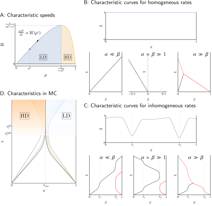
Figure S5: (Related to Phase transitions and profiles. of STAR Methods). $H(\rho)$ and its effect on characteristic curves. A: The rate-normalized flux $H(\rho)=J(\rho,x)/\lambda(x)$ is depicted in solid blue and orange, with characteristic velocity of $x^{t}$ indicated. If $J(\rho^{0},x^{0})<J_{\max}$, the characteristic density $\rho^{t}$ stays within the regions marked LD (blue) or HD (orange), depending on the sign of $\rho^{0}-(\ell+\sqrt{\ell})^{-1}$. Otherwise, $\rho^{t}$ may cross $(\ell+\sqrt{\ell})^{-1}$ forcing the characteristic $x^{t}$ to return to its origin $x^{0}$. B,C: Characteristic curves starting at lattice start (black solid curves) and end (red solid curves) for different regions of the phase diagram. Dotted curves represent shock fronts, with colors indicating which characteristic drives the shock. B: Homogeneous rates give rise to straight line characteristics with speed $\partial_{\rho}J(\rho_{0})$ and $\partial_{\rho}J(\rho_{1})$, respectively. C: Inhomogeneous rates produce more complicated behavior, with characteristics curves slowing down (and potentially reversing direction) near the troughs ($x_{1}$ and $x_{2}$) of $\lambda$. D: If $J(\rho^{0},x^{0})>J_{\max}$ the characteristic curves $x^{t}$ (left and right colored solid curves) reverse directions at critical times $t_{c}$ and return to their origin. At $t_{c}$, the density $\rho^{t}$ switches from LD (blue) to HD (orange) (if associated with $x^{0}=0$) or HD to LD (if associated with $x^{0}=1$, cf. A). The same happens on all associated rarefaction waves (dashed curves), which interpolate between $x^{t}$ and the stationary shock of $x_{\max}^{t}$ (solid black curve).

(17) has two solutions (see Figure S5A) of the form

$$\rho_{\pm}(x)=\dfrac{1}{2\ell}+\dfrac{J_{c}(\ell-1)}{2\ell\lambda(x)}\pm\sqrt{\bigg{(}\dfrac{1}{2\ell}+\dfrac{J_{c}(\ell-1)}{2\ell\lambda(x)}\bigg{)}^{2}-\dfrac{J_{c}}{\ell\lambda(x)}},$$ (19)

any mixture of which may be a potential attractor picked by the system as $t\to\infty$. Deciding precisely which mixture dominates requires analysis of the characteristic curves.

Solving the characteristic ODE.

Denoting the characteristic curves by $x^{t}$ and $\rho^{t}$ with initial data $x^{0},\rho^{0}$, their evolution is described by the system of ODE (Evans,, 2010)

$$\frac{dx^{t}}{dt} =\lambda(x^{t})H^{\prime}(\rho^{t}),$$ (20)

$$\frac{d\rho^{t}}{dt} =-\lambda^{\prime}(x^{t})H(\rho^{t}),$$ (21)

where $H^{\prime}$ and $\lambda^{\prime}$ respectively denote the derivatives of $H$ and $\lambda$ with respect to their arguments. The solutions are easily verified to be

$$x^{t} =F^{-1}(t)$$ (22)

$$\rho^{t} =H^{-1}\left(\dfrac{J(\rho^{0},x^{0})}{\lambda(x^{t})}\right)$$ (23)

as long as $J(\rho^{0},x^{0})\in[0,J_{\max}]$. The form of $F$ follows from formally separating variables:

$$F(x)=\int_{x^{0}}^{x}\dfrac{1}{\lambda(y)H^{\prime}\circ H^{-1}(J(\rho^{0},x^{0})/\lambda(y))}\ \mathrm{d}y,$$ (24)

while $H^{-1}(J(\rho^{0},x^{0})/\lambda(x^{t}))$ is understood to be the preimage compatible with $\rho^{0}$, see Figure S5A. For the homogeneous $\ell$-TASEP (22) and (23) depend linearly on each other, giving rise to straight line characteristic curves (see Figure S5B). In the more general heterogeneous setting, however, more complicated behavior emerges (Figure S5C). In particular, if $J(\rho^{0},x^{0})<J_{\max}$, then for all $t\geq 0$,

$$\frac{J(\rho^{0},x^{0})}{\lambda(x^{t})}<\frac{1}{(1+\sqrt{\ell})^{2}},$$

so $\rho^{t}<\frac{1}{\ell+\sqrt{\ell}}$ for all $t$ if $\rho^{0}<\frac{1}{\ell+\sqrt{\ell}}$, while $\rho^{t}>\frac{1}{\ell+\sqrt{\ell}}$ for all $t$ if $\rho^{0}>\frac{1}{\ell+\sqrt{\ell}}$. Hence, the sign of $\frac{dx^{t}}{dt}=\lambda(x^{t})H^{\prime}(\rho^{t})$ remains the same for all $t$, and any characteristic curve $x^{t}$ starting at the left lattice boundary $x^{0}=0$ or right lattice boundary $x^{0}=1$ propagates towards the opposite end and fills the lattice entirely.

On the other hand, if $J(\rho^{0},x^{0})>J_{\max}$, then $\frac{J(\rho^{0},x^{0})}{\lambda(x_{\min})}>\frac{1}{(1+\sqrt{\ell})^{2}}$, where $x_{\mathrm{min}}=\arg\min_{x}\lambda(x)$, so $H^{-1}\Big{(}\frac{J(\rho^{0},x^{0})}{\lambda(x_{\min})}\Big{)}>\frac{1}{\ell}$. Recalling (23) and noting that it is physically not possible to have $\rho^{t}>\frac{1}{\ell}$, we conclude that the characteristic curve $x^{t}$ cannot reach $x_{\min}$. Indeed, it follows from (20) and (21) that at some critical time $t_{c}$ before reaching $x_{\min}$, the characteristic curve $x^{t}$ reverses direction while $\rho^{t}$ crosses $\arg\max_{\rho}H(\rho)=(\ell+\sqrt{\ell})^{-1}$, resulting in $x^{t}$ returning to its origin. Figure 1E of the main text and Figure S5D illustrate this behavior.

Computing initial densities $\rho^{0}$.

As a consequence of the above, determining phase transitions in the $\alpha$-$\beta$ phase diagram reduces to establishing regimes in which $J(\rho^{0},x^{0})$ exceeds or falls short of $J_{\max}$, which in turn is equivalent to finding an expression for $\rho^{0}$ in terms of $\alpha$ and $\beta$. This is done by considering each lattice end separately and balancing currents:

The right lattice end $x^{0}=1$: As described in the main text, $\rho_{1}=\rho(1)$ decomposes into a sum of two contributions, the periodic part $\rho_{1}^{+}$ and the troughs $\rho_{1}^{-}$ (Chou and Lakatos,, 2004). More explicitly,

$$\rho_{1}=\dfrac{1}{\ell}\bigg{[}(\ell-1)\rho_{1}^{-}+\rho_{1}^{+}\bigg{]}.$$ (25)

Since the current $J_{c}$ is a conserved quantity of the system, the local currents across the last lattice site, the second to last lattice site and within the last $\ell$ sites must all be the same:

$$J_{R}:=J(\rho_{1},1)=\beta\rho_{1}^{+}=\lambda_{1}\rho_{1}^{-}.$$ (26)

Solving for $\rho_{1}$ gives exactly $\frac{1}{\ell}(1-\frac{\beta}{\lambda_{1}})$. Consequently, $J_{R}\leq J_{\max}$ iff

$$\beta<\beta^{\ast}=\frac{1}{2}\Bigg{[}\lambda_{1}-\frac{\ell-1}{(1+\sqrt{\ell})^{2}}\lambda_{\mathrm{min}}-\sqrt{\left(\lambda_{1}-\frac{\ell-1}{(1+\sqrt{\ell})^{2}}\lambda_{\mathrm{min}}\right)^{2}-\frac{4\lambda_{1}\lambda_{\mathrm{min}}}{(1+\sqrt{\ell})^{2}}}\;\Bigg{]}.$$ (27)

The left lattice end $x^{0}=0$: Computing $\alpha^{\ast}$ is more delicate as the effective jump rate is a combination of entrance rate and particle exclusion. To bypass this problem, we investigate the current of holes rather than particles, which is running in the opposite direction. With the loss of the particle-hole symmetry present in the simple $1$-TASEP (Derrida et al.,, 1993), the hole density $\rho^{h}$ here assumes a more complicated form. It satisfies its own conservation law given by

$$\partial_{t^{h}}\rho^{h}=\partial_{x}[J^{h}(\rho^{h},x)],$$ (28)

where

$$J^{h}(\rho^{h},x)=\lambda(x)\rho^{h}\dfrac{1-\rho^{h}}{1+(\ell-1)\rho^{h}}$$ (29)

and $t^{h}=\ell t$ is the time scale of the holes, moving slower as their density is higher. Thus by balancing hole currents rather than particle currents at $x^{0}=0$, we obtain, noting that the effective exit rate (of holes) is still $\alpha$ (as $\ell$ holes need to accumulate for exiting to happen),

$$J^{h}(\rho_{0}^{h},0)=\alpha\rho_{0}^{h}.$$ (30)

Solving for $\rho_{0}^{h}$ and using $\rho_{0}^{h}=1-\ell\rho_{0}$, we obtain $\rho_{0}=\alpha/[\lambda_{0}+(\ell-1)\alpha]$. Defining $J_{L}:=J(\rho_{0},0)$, we obtain $\alpha^{\ast}$ by solving for $\alpha,\ J_{L}=J_{\max}$.

Phase transitions and profiles.

Using the densities obtained from (26) and (30) in the characteristic curves (20) and (21) yields the HD and LD regimes for parameter configurations $(\alpha>\alpha^{\ast},\beta<\beta^{\ast})$ and $(\alpha<\alpha^{\ast},\beta>\beta^{\ast})$, respectively. To describe the phase transition between HD and LD, we observe that for $\alpha<\alpha^{\ast}$ and $\beta<\beta^{\ast}$ both characteristic curves move into the lattice, meet, and move along a common shock with speed

$$v_{\mathrm{shock}}=\dfrac{J_{R}-J_{L}}{\rho_{r}-\rho_{l}},$$ (31)

where $\rho_{l}$ and $\rho_{r}$ are the densities left and right of the shock. As $\rho_{r}-\rho_{l}>0$ as long as $\alpha<\alpha^{\ast}$ and $\beta<\beta^{\ast}$ (cf. Figure S5A), $v_{\mathrm{shock}}>0$ if and only if $J_{R}>J_{L}$. That is, the slower current pushes the faster one past the lattice boundaries and dominates the stationary behavior of the system. The HD and LD regimes are thus separated by incoming currents of equal magnitudes

$$J_{L}=\dfrac{\alpha(\lambda_{0}-\alpha)}{\lambda_{0}+(\ell-1)\alpha}=\dfrac{\beta(\lambda_{1}-\beta)}{\lambda_{1}+(\ell-1)\beta}=J_{R}.$$ (32)

Lastly, we can use the behavior of characteristic curves for $J(\rho^{0},x^{0})>J_{\max}$ to describe stationary profiles in the MC regime ($\alpha>\alpha^{\ast}$ and $\beta>\beta^{\ast}$): Each characteristic curve reverses direction at a critical time $t_{c}$ and returns to its respective lattice boundary, while the density $\rho^{t}$ it carries transitions from $\rho_{-}$ to $\rho_{+}$ (on the left characteristic) or $\rho_{+}$ to $\rho_{-}$ (on the right characteristic). Since the reversal of directions occurs strictly before reaching $x_{\min}$, these characteristics provide density information on only part of the lattice. The uncovered regions are determined by the simultaneously propagating rarefaction waves (Evans,, 2010), which interpolate between $x^{t}$ and the characteristic curve $x_{\max}^{t}$ associated with $J(\rho^{0},x^{0})=J_{\max}$ (see Figure S5D). Together, these observations combine to produce the high density and low density profiles to the left and right of $x_{\min}$, respectively, with critical current $J_{c}=J_{\max}$, as described in the main manuscript.

If $\lambda$ has exactly one global minimum $x_{\min}$, this description captures the density profile on the entire lattice. In the case of multiple global minima at $\{x_{\min,1},\ldots,x_{\min,n}\}$ however, it describes $\rho$ on $[0,x_{\min,1}]\,\cup\,[x_{\min,n},1]$ only, leaving open fluctuations on the middle segment $(x_{\min,1},x_{\min,n})$. Although unlikely to be encountered in practice, these singular rate functions exhibit interesting stochastic phenomena: The presence of high densities on the initial interval and low densities on the terminal one suggest the formation of a coexistence phase in-between. Indeed, the subsystem restricted to $[x_{\min,1},x_{\min,n}]$ may be regarded as a TASEP with entrance and exit rates $\alpha=\beta=\lambda_{\min}/(1+\sqrt{\ell})$, positioning it at the triple point of the phase diagram, and computing the characteristics reveals one or multiple stationary shock fronts in the interior. Such macroscopic phenomenon in the homogeneous $1$-TASEP has previously been associated on the microscopic level with a shock performing a random walk on the lattice with reflecting boundaries (Derrida et al.,, 1997). Numerical simulations seem to locate these shock around local maxima disproportionately often (cf. Figure S2), which might reflect dependencies of its diffusivity on $\lambda$.

Applicability to discrete lattices

The existence of a continuous limiting rate function $\lambda:[0,1]\to\mathbb{R}^{+}$ extending the discrete jump rates $p_{k}=\lambda(ak)$ is an important ingredient in our treatment of the hydrodynamic limit. That is, in order for density profiles to be accurately approximated by solutions to the PDE (3), the $p_{k}$ must vary smoothly across lattice sites. Microscopic systems like the translation machinery in cells, however, are typically subjected to substantial amounts of fluctuations, resulting in far rougher elongation profiles (see Figure 2A). Despite this lack of regularity, the hydrodynamic limit can still be employed to describe local averages of such a system. More precisely, fixing $r\in\{1,\dots,N\}$, we associate with an elongation rate profile $\{p_{1},\dots,p_{N}\}$ and the corresponding density profile $\{\rho_{1},\dots,\rho_{N}\}$ their smoothed profiles $\{\overline{p}_{1},\dots,\overline{p}_{N-r+1}\}$ and $\{\overline{\rho}_{1},\dots,\overline{\rho}_{N-r+1}\}$, respectively, obtained through a moving $r$-codon average: $\overline{p}_{k}=\sum_{i=k}^{k+r-1}p_{i}/r$, and $\overline{\rho}_{k}=\sum_{i=k}^{k+r-1}\rho_{i}/r$. Moreover, we define $\{\sigma_{1},\dots,\sigma_{N-r+1}\}$ to be the steady state density profile under the elongation rates $\{\overline{p}_{k}\}$. If $\{p_{k}\}$ extends to a smooth $\lambda:[0,1]\to\mathbb{R}^{+}$, then since $|\overline{p}_{k}-p_{k}|\in O(N^{-1})$, $\{\overline{p}_{k}\}$ extends to this same $\lambda$, and hence $\{\rho_{k}\},\{\overline{\rho}_{k}\}$ and $\{\sigma_{k}\}$ all converge to the solution $\rho$ of (3). When $\{p_{k}\}$ does not extend to a continuous limit, then $\{\rho_{k}\}$ generally does not either. However, by the same reasoning that establishes the hydrodynamics for the $1$-TASEP with quenched disorder (Seppäläinen et al.,, 1999), $\{\overline{\rho}_{k}\}$ should still be close to $\{\sigma_{k}\}$, which, due to the greater regularity of $\{\overline{p}_{k}\}$, is well approximated by the hydrodynamic density profile under $\{\overline{p}_{k}\}$. Thus, $\{\overline{\rho}_{k}\}$ is ultimately well approximated by the hydrodynamic limit under $\{\overline{p}_{k}\}$.

To confirm this, we carried out an extensive simulation study on elongation rate profiles obtained from ribosome profiling data of yeast (see Data processing for more details on data). Specifically, we performed the smoothing $\{p_{k}\}\to\{\overline{p}_{k}\}$ (Figure 2A,B), simulated density profiles $\{\rho_{k}\}$ under $\{p_{k}\}$ (Figure 2A,C), and compared the corresponding smoothed densities $\{\overline{\rho}_{k}\}$ with the hydrodynamic prediction under $\{\overline{p}_{k}\}$ (Figure 2D). A choice of $r=10$, which is equal to the particle (ribosome) size $\ell$ in translation and the smallest window size guaranteeing smoothness of $\{\overline{p}_{k}\}$ due to the $\ell$-periodicity induced by traffic jams, resulted in excellent agreement both in densities and currents uniformly across transcripts while maintaining local structure.

Boundary conditions

The computation of initial densities in Solving the characteristic ODE. yielded precise boundary values for $x=0$ in the LD regime and $x=1$ in the HD regime, respectively. Using the same principle of balancing currents, boundary conditions for all locations in the phase diagram can be computed. The results are listed in Table S1, which extend previous results obtained in (Lakatos and Chou,, 2003) (who derived entries (1,1), (2,2) and (2,3) of Table S1). More precise information about the boundary layers can be gleaned from direct analysis of (15) rather than its limit (16).

Data processing

Initiation, elongation, and termination rates were obtained from an earlier work (Dao Duc and Song,, 2018), where the rates were estimated from ribosome profiling data of S. cerevisiae for a set of 850 genes selected based on length and footprint coverage. The initiation and termination rates ($\alpha$ and $\beta$) were taken directly from that previous work. To compute the elongation rates relevant to the hydrodynamic limit, we applied a ten-codon moving average to their elongation rates (see Applicability to discrete lattices). To demonstrate replicability on larger datasets, we took ribosome profiles directly from Williams et al., (2014) and Pop et al., (2014) (combined with polysome profiling from MacKay et al., (2004) for normalization purposes, yielding 3098 and 2536 genes, respectively), smoothed them by moving averages of length $\ell=10$, and inverted the solution of (3) to obtain initiation rates, termination rates, and smoothed elongation profiles.

QUANTIFICATION AND STATISTICAL ANALYSIS

Hypothesis tests and $p$-values

To establish significance of a subset $X$ of genes with respect to a statistic $f$ (e.g., $\alpha,J$ or $x_{\min}$) relative to a background set $Y$, we performed hypothesis testing on the median $m_{f}$ of $f$ over samples in $X$. Under the null distribution of $X$ being drawn uniformly at random, the probability of this test statistic exceeding $m$ equals the probability of a hypergeometric variable with parameters $N=\left|Y\right|,K=2\left|Y_{m}\right|,n=\left|X\right|$, where $Y_{m}$ is the set of genes in $Y$ whose $f$ exceeds $m$, exceeding $\lfloor\left|X/2\right|\rfloor$. This p-value can be computed explicitly. Sets of ribosomal and stress response genes were taken from the Saccharomyces Genome Database (Cherry et al.,, 2011).

Agreement between theoretical prediction and simulation

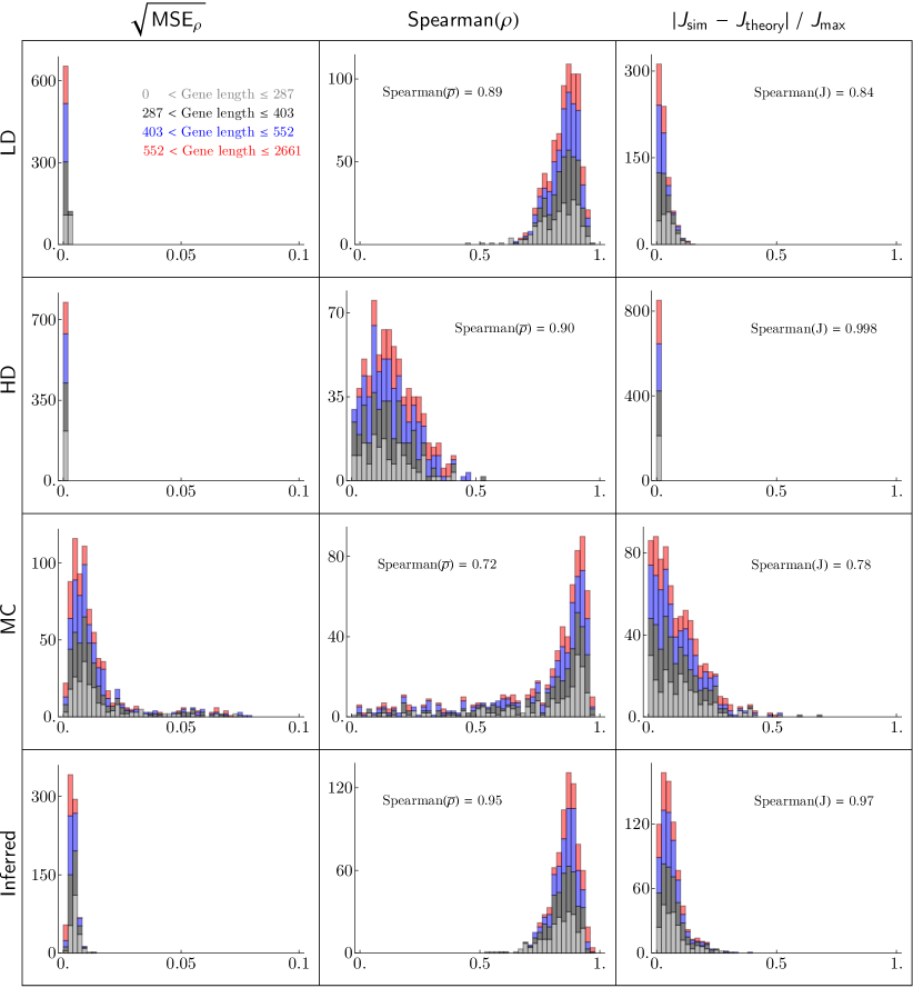
Figure S6: (Related to Agreement between theoretical prediction and simulation of STAR Methods). Comparison between simulation and theoretical prediction of our hydrodynamic approximation. Absolute errors in position-specific ribosome densities $\rho$ (first column) and currents $J$ (third column) are low for all gene lengths (colored), for different regimes in the phase diagram (first three rows), and for biologically relevant initiation and termination rates (last row) inferred in Dao Duc and Song, (2018). Moreover, transcript-by-transcript ribosome density profiles $\rho$ and mean ribosome occupancies $\overline{\rho}$ correlate well between simulated data and our hydrodynamic predictions (middle column), as does currents (figure inset in third column).

In order to empirically verify our theoretical justification of the hydrodynamic limit, we simulated ribosome profiles and currents for all 850 S. cerevisiae genes studied in Dao Duc and Song, (2018). For each gene, we considered four conditions: LD, HD, MC, and under the actual initiation and termination rates inferred in Dao Duc and Song, (2018); these four conditions correspond to different rows in Figure S6. Absolute errors in ribosome density profiles and currents (first and last columns of Figure S6) are accurately predicted across all gene lengths—with a slight increase in prediction accuracy for longer genes (as expected, since the hydrodynamic limit becomes exact in the infinite length limit)—and across all regimes of the phase diagram. Due to two or more bottlenecks occasionally competing on the same transcript (i.e., when $|\{x\ :\ \lambda(x)=\lambda_{\min}\}|>1$, cf. last paragraph of Phase transitions and profiles. of STAR Methods), error distributions in MC exhibit heavier tails than in LD and HD. However, overall these outliers do not affect the quality of our theoretical prediction significantly. In particular, correlations between simulated and theoretical transcript-by-transcript quantities—ribosome density profiles and mean occupancies (middle column), as well as currents (last column)—are consistently high, demonstrating good predictive power of our hydrodynamic framework.

In HD, predicted and simulated ribosome density profiles had quite low mean squared differences (second row, first column of Figure S6), but poor correlation (histograms in second row, second column). This seemingly contradictory result can be explained by typical fluctuations in theoretical density profiles being of the same order as typical fluctuations in the random noise (mean ratio of fluctuations $=0.037$). That is, generic HD profiles are close to flat, allowing uncorrelated site-by-site noise to substantially reduce overall correlations.

DATA AND CODE AVAILABILITY

This study did not generate new data. Code, including the code used to generate all figures, is publicly available at https://github.com/songlab-cal/l-TASEP.

Supplementary Figures and Table

Table S1: (Related to Boundary conditions of STAR Methods). Boundary conditions by phase. Expected densities at the left ($x=0$) and right ($x=1$) end boundaries of the lattice.

Phase	$\rho_{0}$	$\rho_{1}^{+}$	$\rho_{1}^{-}$
LD	$\dfrac{\alpha}{\lambda_{0}+(\ell-1)\alpha}$	$\dfrac{1}{\beta}\bigg{[}\dfrac{\alpha(\lambda_{0}-\alpha)}{\lambda_{0}+(\ell-1)\alpha}\bigg{]}$	$\dfrac{1}{\lambda_{1}}\bigg{[}\dfrac{\alpha(\lambda_{0}-\alpha)}{\lambda_{0}+(\ell-1)\alpha}\bigg{]}$
HD	$\dfrac{1}{\ell}-\dfrac{1}{\ell\alpha}\bigg{[}\dfrac{\beta(\lambda_{1}-\beta)}{\lambda_{1}+(\ell-1)\beta}\bigg{]}$	$\dfrac{\lambda_{1}-\beta}{\lambda_{1}+(\ell-1)\beta}$	$\dfrac{1}{\lambda_{1}}\bigg{[}\dfrac{\beta(\lambda_{1}-\beta)}{\lambda_{1}+(\ell-1)\beta}\bigg{]}$
MC	$\dfrac{1}{\ell}-\dfrac{1}{\ell\alpha}\bigg{[}\dfrac{\lambda_{\min}}{(1+\sqrt{\ell})^{2}}\bigg{]}$	$\dfrac{1}{\beta}\bigg{[}\dfrac{\lambda_{\min}}{(1+\sqrt{\ell})^{2}}\bigg{]}$	$\dfrac{1}{\lambda_{1}}\bigg{[}\dfrac{\lambda_{\min}}{(1+\sqrt{\ell})^{2}}\bigg{]}$

REFERENCES

- Bahadoran, (2012) Bahadoran, C. (2012). Hydrodynamics and hydrostatics for a class of asymmetric particle systems with open boundaries. Communications in Mathematical Physics, 310(1):1–24.
- Ben-Yehezkel et al., (2015) Ben-Yehezkel, T., Atar, S., Zur, H., Diament, A., Goz, E., Marx, T., Cohen, R., Dana, A., Feldman, A., Shapiro, E., et al. (2015). Rationally designed, heterologous s. cerevisiae transcripts expose novel expression determinants. RNA biology, 12(9):972–984.
- Blythe and Evans, (2007) Blythe, R. A. and Evans, M. R. (2007). Nonequilibrium steady states of matrix-product form: a solver’s guide. Journal of Physics A: Mathematical and Theoretical, 40(46):R333–R441.
- Boël et al., (2016) Boël, G., Letso, R., Neely, H., Price, W. N., Wong, K.-H., Su, M., Luff, J. D., Valecha, M., Everett, J. K., Acton, T. B., et al. (2016). Codon influence on protein expression in E. coli correlates with mRNA levels. Nature, 529(7586):358–363.
- Cherry et al., (2011) Cherry, J. M., Hong, E. L., Amundsen, C., Balakrishnan, R., Binkley, G., Chan, E. T., Christie, K. R., Costanzo, M. C., Dwight, S. S., Engel, S. R., et al. (2011). Saccharomyces Genome Database: the genomics resource of budding yeast. Nucleic Acids Research, 40(D1):D700–D705.
- Chou and Lakatos, (2004) Chou, T. and Lakatos, G. (2004). Clustered bottlenecks in mRNA translation and protein synthesis. Phys. Rev. Lett., 93:198101.
- Covert and Rezakhanlou, (1997) Covert, P. and Rezakhanlou, F. (1997). Hydrodynamic limit for particle systems with nonconstant speed parameter. Journal of statistical physics, 88(1):383–426.
- Dao Duc and Song, (2018) Dao Duc, K. and Song, Y. S. (2018). The impact of ribosomal interference, codon usage, and exit tunnel interactions on translation elongation rate variation. PLoS Genetics, 14(e1007166):1–32.
- Derrida et al., (1993) Derrida, B., Evans, M. R., Hakim, V., and Pasquier, V. (1993). Exact solution of a 1D asymmetric exclusion model using a matrix formulation. Journal of Physics A: Mathematical and General, 26(7):1493–1517.
- Derrida et al., (1997) Derrida, B., Lebowitz, J., and Speer, E. (1997). Shock profiles for the asymmetric simple exclusion process in one dimension. Journal of Statistical Physics, 89(1-2):135–167.
- Dever et al., (2016) Dever, T. E., Kinzy, T. G., and Pavitt, G. D. (2016). Mechanism and regulation of protein synthesis in Saccharomyces cerevisiae. Genetics, 203(1):65–107.
- Dong et al., (2007) Dong, J. J., Schmittmann, B., and Zia, R. K. P. (2007). Inhomogeneous exclusion processes with extended objects: The effect of defect locations. Phys. Rev. E, 76:051113.
- Evans, (2010) Evans, L. C. (2010). Partial Differential Equations, Vol. 19 of Graduate Studies in Mathematics American Mathematical Society. American Mathematical Society, Providence, Rhode Island.
- Frumkin et al., (2018) Frumkin, I., Lajoie, M. J., Gregg, C. J., Hornung, G., Church, G. M., and Pilpel, Y. (2018). Codon usage of highly expressed genes affects proteome-wide translation efficiency. Proceedings of the National Academy of Sciences, 115(21):E4940–E4949.
- Frumkin et al., (2017) Frumkin, I., Schirman, D., Rotman, A., Li, F., Zahavi, L., Mordret, E., Asraf, O., Wu, S., Levy, S. F., and Pilpel, Y. (2017). Gene architectures that minimize cost of gene expression. Molecular Cell, 65(1):142–153.
- Gilchrist, (2007) Gilchrist, M. A. (2007). Combining models of protein translation and population genetics to predict protein production rates from codon usage patterns. Molecular Biology and Evolution, 24(11):2362–2372.
- Gustafsson et al., (2012) Gustafsson, C., Minshull, J., Govindarajan, S., Ness, J., Villalobos, A., and Welch, M. (2012). Engineering genes for predictable protein expression. Protein Expression and Purification, 83(1):37–46.
- Hanson and Coller, (2018) Hanson, G. and Coller, J. (2018). Codon optimality, bias and usage in translation and mRNA decay. Nature Reviews Molecular Cell Biology, 19(1):20–30.
- Hershberg and Petrov, (2008) Hershberg, R. and Petrov, D. A. (2008). Selection on codon bias. Annual Review of Genetics, 42:287–299.
- Humphreys et al., (2005) Humphreys, D. T., Westman, B. J., Martin, D. I., and Preiss, T. (2005). MicroRNAs control translation initiation by inhibiting eukaryotic initiation factor 4E/cap and poly(A) tail function. Proceedings of the National Academy of Sciences, 102(47):16961–16966.
- Katranidis and Fitter, (2019) Katranidis, A. and Fitter, J. (2019). Single-molecule techniques and cell-free protein synthesis: A perfect marriage. Analytical Chemistry, 91(4):2570–2576.
- Kipnis and Landim, (2013) Kipnis, C. and Landim, C. (2013). Scaling limits of interacting particle systems, volume 320. Springer Science & Business Media.
- Kosuri et al., (2013) Kosuri, S., Goodman, D. B., Cambray, G., Mutalik, V. K., Gao, Y., Arkin, A. P., Endy, D., and Church, G. M. (2013). Composability of regulatory sequences controlling transcription and translation in Escherichia coli. Proceedings of the National Academy of Sciences, 110(34):14024–14029.
- Kristensen et al., (2013) Kristensen, A. R., Gsponer, J., and Foster, L. J. (2013). Protein synthesis rate is the predominant regulator of protein expression during differentiation. Molecular Systems Biology, 9(689):1–12.
- Lakatos and Chou, (2003) Lakatos, G. and Chou, T. (2003). Totally asymmetric exclusion processes with particles of arbitrary size. Journal of Physics A: Mathematical and General, 36(8):2027–2041.
- Levin and Tuller, (2018) Levin, D. and Tuller, T. (2018). Genome-scale analysis of perturbations in translation elongation based on a computational model. Scientific reports, 8(1):16191.
- Lu et al., (2007) Lu, P., Vogel, C., Wang, R., Yao, X., and Marcotte, E. M. (2007). Absolute protein expression profiling estimates the relative contributions of transcriptional and translational regulation. Nature Biotechnology, 25(1):117–124.
- MacDonald et al., (1968) MacDonald, C. T., Gibbs, J. H., and Pipkin, A. C. (1968). Kinetics of biopolymerization on nucleic acid templates. Biopolymers, 6(1):1–25.
- MacKay et al., (2004) MacKay, V. L., Li, X., Flory, M. R., Turcott, E., Law, G. L., Serikawa, K. A., Xu, X., Lee, H., Goodlett, D. R., Aebersold, R., et al. (2004). Gene expression analyzed by high-resolution state array analysis and quantitative proteomics response of yeast to mating pheromone. Molecular & Cellular Proteomics, 3(5):478–489.
- Mahajan and Agashe, (2018) Mahajan, S. and Agashe, D. (2018). Translational selection for speed is not sufficient to explain variation in bacterial codon usage bias. Genome Biology and Evolution, 10(2):562–576.
- Moore et al., (2017) Moore, S. J., MacDonald, J. T., and Freemont, P. S. (2017). Cell-free synthetic biology for in vitro prototype engineering. Biochemical Society Transactions, 45(3):785–791.
- Plotkin and Kudla, (2011) Plotkin, J. B. and Kudla, G. (2011). Synonymous but not the same: the causes and consequences of codon bias. Nature Reviews Genetics, 12(1):32–42.
- Pop et al., (2014) Pop, C., Rouskin, S., Ingolia, N. T., Han, L., Phizicky, E. M., Weissman, J. S., and Koller, D. (2014). Causal signals between codon bias, mrna structure, and the efficiency of translation and elongation. Molecular Systems Biology, 10(12):770.
- Quax et al., (2015) Quax, T. E., Claassens, N. J., Söll, D., and van der Oost, J. (2015). Codon bias as a means to fine-tune gene expression. Molecular Cell, 59(2):149–161.
- Rezakhanlou, (1991) Rezakhanlou, F. (1991). Hydrodynamic limit for attractive particle systems on . Communications in Mathematical Physics, 140(3):417–448.
- Rosenblum and Cooperman, (2014) Rosenblum, G. and Cooperman, B. S. (2014). Engine out of the chassis: Cell-free protein synthesis and its uses. FEBS letters, 588(2):261–268.
- Salis et al., (2009) Salis, H. M., Mirsky, E. A., and Voigt, C. A. (2009). Automated design of synthetic ribosome binding sites to control protein expression. Nature Biotechnology, 27(10):946–950.
- Schönherr, (2005) Schönherr, G. (2005). Hard rod gas with long-range interactions: Exact predictions for hydrodynamic properties of continuum systems from discrete models. Phys. Rev. E, 71:026122.
- Schönherr and Schütz, (2004) Schönherr, G. and Schütz, G. (2004). Exclusion process for particles of arbitrary extension: hydrodynamic limit and algebraic properties. Journal of Physics A: Mathematical and General, 37(34):8215–8231.
- Seppäläinen et al., (1999) Seppäläinen, T. et al. (1999). Existence of hydrodynamics for the totally asymmetric simple k-exclusion process. The Annals of Probability, 27(1):361–415.
- Shah et al., (2013) Shah, P., Ding, Y., Niemczyk, M., Kudla, G., and Plotkin, J. B. (2013). Rate-limiting steps in yeast protein translation. Cell, 153(7):1589–1601.
- Shaw et al., (2004) Shaw, L. B., Sethna, J. P., and Lee, K. H. (2004). Mean-field approaches to the totally asymmetric exclusion process with quenched disorder and large particles. Phys. Rev. E, 70:021901.
- Shaw et al., (2003) Shaw, L. B., Zia, R., and Lee, K. H. (2003). Totally asymmetric exclusion process with extended objects: a model for protein synthesis. Physical Review E, 68(2):021910(17).
- Stinchcombe and de Queiroz, (2011) Stinchcombe, R. B. and de Queiroz, S. L. A. (2011). Smoothly varying hopping rates in driven flow with exclusion. Physical Review E, 83:061113.
- Szavits-Nossan et al., (2018) Szavits-Nossan, J., Ciandrini, L., and Romano, M. C. (2018). Deciphering mRNA sequence determinants of protein production rate. Phys. Rev. Lett., 120:128101.
- Tuller et al., (2010) Tuller, T., Carmi, A., Vestsigian, K., Navon, S., Dorfan, Y., Zaborske, J., Pan, T., Dahan, O., Furman, I., and Pilpel, Y. (2010). An evolutionarily conserved mechanism for controlling the efficiency of protein translation. Cell, 141(2):344–354.
- Williams et al., (2014) Williams, C. C., Jan, C. H., and Weissman, J. S. (2014). Targeting and plasticity of mitochondrial proteins revealed by proximity-specific ribosome profiling. Science, 346(6210):748–751.
- Wyant et al., (2018) Wyant, G. A., Abu-Remaileh, M., Frenkel, E. M., Laqtom, N. N., Dharamdasani, V., Lewis, C. A., Chan, S. H., Heinze, I., Ori, A., and Sabatini, D. M. (2018). NUFIP1 is a ribosome receptor for starvation-induced ribophagy. Science, 360:751–758.
- Yu et al., (2015) Yu, C.-H., Dang, Y., Zhou, Z., Wu, C., Zhao, F., Sachs, M. S., and Liu, Y. (2015). Codon usage influences the local rate of translation elongation to regulate co-translational protein folding. Molecular Cell, 59(5):744–754.
- Zia et al., (2011) Zia, R. K., Dong, J., and Schmittmann, B. (2011). Modeling translation in protein synthesis with TASEP: A tutorial and recent developments. Journal of Statistical Physics, 144(2):405–428.
- Zur and Tuller, (2016) Zur, H. and Tuller, T. (2016). Predictive biophysical modeling and understanding of the dynamics of mrna translation and its evolution. Nucleic Acids Research, 44(19):9031–9049.