Excited States of Methylene, Polyenes, and Ozone
from Heat-bath Configuration Interaction

Abstract

The electronically excited states of methylene (CH₂), ethylene (C₂H₄), butadiene (C₄H₆), hexatriene (C₆H₈), and ozone (O₃) have long proven challenging due to their complex mixtures of static and dynamic correlations. Semistochastic heat-bath configuration interaction (SHCI), which efficiently and systematically approaches the full configuration interaction (FCI) limit, is used to provide close approximations to the FCI energies in these systems. This article presents the largest FCI-level calculation to date – on hexatriene using a polarized double-zeta basis (ANO-L-pVDZ), which gives rise to a Hilbert space containing more than $10^{38}$ determinants. These calculations give vertical excitation energies of 5.58 and 5.59 eV respectively for the $2^{1}{\rm A}_{\rm g}$ and $1^{1}{\rm B}_{\rm u}$ states, showing that they are nearly degenerate. The same excitation energies in butadiene/ANO-L-pVDZ were found to be 6.58 and 6.45 eV. In addition to these benchmarks, our calculations strongly support the presence of a previously hypothesized ring-minimum species of ozone that lies 1.3 eV higher than the open-ring minimum energy structure and is separated from it by a barrier of 1.11 eV.

I Introduction

The exponential increase in Hamiltonian dimension with increasing system size means that exact, Born-Oppenheimer electronic energies are not easily achievable for polyatomic molecular systems. Knowles1984 ; Olsen1988 ; Olsen1990 ; Olsen1996 ; Rossi1999 ; Dutta2003 ; Gan2006 Recent years have seen impressive progress in methods that produce FCI-quality energies at greatly reduced cost, such as density matrix renormalization group (DMRG), White1993 ; White1999 ; Chan2002 ; Chan2011 ; Olivares-Amaya2015 FCI quantum Monte Carlo (FCIQMC), Booth2009 ; Cleland2010 ; PetHolChaNigUmr-PRL-12 ; Booth2013 and incremental FCI (iFCI). Zimmerman2017 ; Zimmerman2017a ; Zimmerman2017b

Another avenue for obtaining FCI-quality energies has also recently become available due to the revival of the selected configuration interaction plus perturbation theory (SCI+PT) algorithms. SCI+PT consists of two steps. In the first step, the most important determinants of the wavefunction of interest are identified iteratively and the Hamiltonian in this subspace ($\mathcal{V}$) is diagonalized to obtain the approximate variational energies and wavefunctions. In the second step, the perturbative step of SCI+PT attempts to correct these energies and wavefunctions. The first such SCI+PT method was called Configuration Interaction by Perturbatively Selecting Iteratively (CIPSI), which established the basic steps of the SCI+PT algorithms. Huron1973 ; Buenker1975 ; Buenker1978 ; Evangelisti1983 ; Harrison1991 ; BenAmor2011 Since then, many variations of CIPSI have been developed over the years, BuePey-TCA-74 ; langlet1976excited ; oliveros1978ci ; cimiraglia1985second ; cimiraglia1987recent ; Knowles89 ; Har-JCP-91 ; povill1992treating ; SteWenWilWil-CPL-94 ; GarCasCabMal-CPL-95 ; WenSteWil-IJQC-96 ; Neese-JCP-03 ; NakEha-JCP-05 ; AbrShe-CPL-05 ; BytRue-CP-09 ; Rot-PRC-09 ; Eva-JCP-14 ; Kno-MP-15 ; SchEva-JCP-16 ; LiuHof-JCTC-16 ; zhang2016deterministic ; scemama2016quantum ; garniron2017hybrid ; giner2017jeziorski ; schriber2017adaptive all of which try to improve upon the CIPSI algorithm. However, a common drawback of all these variants is that, to construct the selected space $\mathcal{V}$ iteratively, the algorithm has to loop over all the determinants connected to any determinant in previous iteration of $\mathcal{V}$. This becomes prohibitively expensive as the size of space $\mathcal{V}$ increases to several million determinants. Some of us have recently proposed the Heat-bath CI (HCI) Holmes2016 algorithm that eliminates this expensive step by changing the selection criterion such that it enables an algorithm that loops over only those determinants that will be included in the selected space $\mathcal{V}$, a small fraction of all the possible connected determinants. This results in orders of magnitude speed up over other variants of SCI+PT for this step of the algorithm. HCI was further improved by semistochastic evaluation of the pertubative energy in semistochastic HCI (SHCI), Sharma2017 which eliminated the need to store a long list of perturbative determinants in memory. SHCI’s potential has been demonstrated in previous works, where it was shown to efficiently treat CI spaces orders of magnitude larger than is possible with conventional CI algorithms. Sharma2017 ; HolUmrSha-JCP-17 ; Smith2017 ; Mussard17

In this paper, highly accurate benchmarks for electronically excited states of the polyatomics in Figure 1 are computed using SHCI. Methylene is presented as the first test case, due to its small size yet challenging electronic structure. Sherrill1998 Additionally, ozone is examined to answer a long-standing question regarding the existence of a theorized meta-stable ozone species. Hay1972 ; Theis2016 Finally, SHCI is applied to the first few polyenes $-$ ethylene, butadiene, and hexatriene $-$ which have long been studied for their role as prototypical organic conducting polymers. The state ordering of the low-lying valence excited states, $2^{1}{\rm A}_{\rm g}$ and $1^{1}{\rm B}_{\rm u}$, in butadiene and hexatriene have been especially challenging due to the significant numbers of highly correlated electrons and the near-degenerate nature of the valence states. Tavan1987 ; Watts1996 ; Starcke2006 ; Li1999 ; Nakayama1998 ; Schreiber2008 ; Mazur2009 ; Schmidt2012 ; Piecuch2015 Herein, extrapolated SHCI state energies will provide high accuracy $2^{1}{\rm A}_{\rm g}$/$1^{1}{\rm B}_{\rm u}$ state orderings in butadiene and hexatriene.

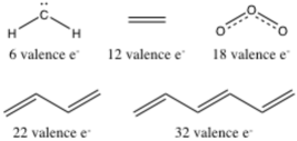
Figure 1: The molecules, methylene, ethylene, ozone, butadiene and hexatriene, investigated with SHCI.

This article is organized as follows. In Section II, the excited-state SHCI algorithm is reviewed, and the path to convergence to the FCI limit is discussed. In Section III, results on the smaller methylene and ethylene systems are used to validate SHCI against current benchmark values and establish convergence with respect to FCI. These observations are then used to estimate FCI-quality energies for the larger ozone, butadiene, and hexatriene molecules. Section IV provides conclusions and an outlook on the SHCI method.

II Methods

II.1 Semistochastic Heat-Bath Configuration Interaction

As HCI and semistochastic perturbation theory have been described in detail, Holmes2016 ; Sharma2017 ; HolUmrSha-JCP-17 only a brief overview will be given here. The HCI algorithm can be divided into variational and perturbative stages, each of which selects determinants through threshold values, $\epsilon_{\rm V}$ and $\epsilon_{\rm PT}$, respectively. The current variational space of determinants is denoted by $\mathcal{V}$ and the space of all determinants connected by single or double excitations to $\mathcal{V}$, but not in $\mathcal{V}$, is denoted by $\mathcal{C}$.

The variational stage iteratively adds determinants to $\mathcal{V}$ by

1. Adding all determinants $a$ connected to determinants in the current $\mathcal{V}$ that pass the importance criterion $\max_{i}\left|H_{ai}\max_{n}\left(\left|c_{i}^{n}\right|\right)\right|>\epsilon_{\rm V}$, where $c_{i}^{n}$ is the coefficient of determinant $i$ in state $n$.

2. Constructing the Hamiltonian and solving for the roots of interest, in the basis of all determinants in the newly expanded $\mathcal{V}$.

3. Repeat 1-2 until convergence.

Convergence of the variational wavefunction for a given $\epsilon_{\rm V}$ is signified by the addition of a small number of new determinants or small changes in the variational energy ($E_{\rm var}$). The second-order Epstein-Nesbet perturbative energy correction ($\Delta E_{2}$) is added to $E_{\rm var}$ to obtain the total HCI energy ($E_{tot}$). This correction is

$$\Delta E_{2}=\sum_{a\in\mathcal{C}}\frac{\left(\sum_{i\in\mathcal{V}}^{(\epsilon_{\rm PT})}H_{ai}c_{i}\right)^{2}}{E_{0}-H_{aa}},$$ (1)

where $a$ runs over determinants in $\mathcal{C}$, and $i$ over determinants in $\mathcal{V}$. Similar to the variational stage, the perturbation only considers the determinants connected to the final $\mathcal{V}$ space that have an importance measure greater than a parameter $\epsilon_{\rm PT}$, which is typically orders of magnitude smaller than $\epsilon_{\rm V}$. In both the variational and the perturbative stages, the fact that the number of distinct values of the double-excitation matrix elements scales only as $N_{\rm orb}^{4}$ is used to avoid ever looking at the unimportant determinants. Nevertheless, storing the full space of determinants used in the perturbative correction becomes a memory bottleneck for larger systems.

SHCI sidesteps this memory bottleneck using a semistochastic second-order perturbation correction. Sharma2017 In this procedure, the perturbative correction is split into deterministic and stochastic contributions. A larger $\epsilon_{\rm PT}^{\rm d}$, automatically determined to correspond to a determinant space of manageable size depending on available computer memory, is first used to obtain a deterministic energy correction. The remaining correlation is then calculated stochastically by taking the difference of the second-order corrections evaluated with $\epsilon_{\rm PT}$ and $\epsilon_{\rm PT}^{\rm d}$. Samples are taken until the statistical error falls below a specified threshold.

II.2 Converging SHCI Energies to the FCI Limit

The target accuracy for total or relative energies are typically be chosen to be 1 mHa or 1.6 mHa (1 kcal/mol, representing chemical accuracy), though for the smaller systems it is easy to achieve much higher accuracy. In SHCI, the error in the variational energy can be straightforwardly estimated by the magnitude of the perturbative correction.

In methylene and ethylene, SHCI can provide such highly converged variational energies. In larger systems, however, converging the variational energy would require prohibitively large variational spaces. Instead, we fit the variational energy or the total energy, $E_{\mathrm{tot}}=E_{\mathrm{var}}+\Delta E_{2}$, to $E_{\mathrm{var}}-E_{\mathrm{tot}}$ using a quadratic function and use the fitted function to extrapolate to the no perturbative correction ($E_{\mathrm{var}}-E_{\mathrm{tot}}=0$) limit. The fit coefficients for variational and total energies are the same, except that the coefficients of the linear terms differ by one, so the two energies extrapolate to precisely the same value. There is not a well-defined method for estimating the extrapolation error, but a reasonable choice is one fifth of the difference between the calculated energy with the smallest value of $\epsilon_{\rm V}$ and the extrapolated energy. In many cases the fitted function is very nearly linear (see e.g. Figs. 2, 4 and 5). Furthermore, even when the fitted functions are not close to linear, the functions for different states are often close to parallel, making the estimates of the energy differences particularly accurate.

II.3 Computational Details

SHCI is implemented in Fortran90, parallelized using MPI, and makes use of spatial symmetry, and time-reversal symmetry when the number of up- and down-spin electrons is equal. Sharma2017 The variational iterations are terminated when when the number of new determinants added is less than 0.001% of the current variational space or when the change in variational energy is less than $1\cdot 10^{-5}$ Ha. For all calculations, $\epsilon_{\rm PT}$ is set to $1\cdot 10^{-7}$ Ha, which provides converged perturbative corrections. Holmes2016 ; Sharma2017 $\epsilon_{\rm V}$ is made as small as possible on our hardware, obtaining either small $\Delta E_{2}$ or enough data points to reliably extrapolate to $\Delta E_{2}=0$. The threshold for statistical error of the stochastic perturbative correction is generally set to $5\cdot 10^{-5}$ Ha, although the larger hexatriene/ANO-L-pVDZ computations use $1\cdot 10^{-4}$ Ha.

For the smaller systems (methylene and ethylene) achieving convergence is relatively easy, allowing the use of Hartree-Fock and HCI natural orbitals (obtained with $\epsilon_{\rm V}=3\cdot 10^{-5}$ Ha), for methylene and ethylene respectively, to construct the molecular orbital integrals. For the larger systems (ozone, butadiene, hexatriene), the convergence was improved by using orbitals that minimize the HCI variational energy Smith2017 for $\epsilon_{\rm V}=2\cdot 10^{-4}$. Possibly, yet better convergence could be obtained by using orbitals that make the total energy stationary Smith2017 .

Basis sets used are aug-cc-pVQZ Dunning1989 ; Kendall1992 for methylene, ANO-L-pVTZ Widmark1990 for ethylene, ANO-L-pVDZ Widmark1990 for butadiene and hexatriene, and cc-pVTZ Dunning1989 for ozone. Geometries for methylene are FCI/TZVP quality taken from Sherrill et al. Sherrill1998 and ozone geometries are CASSCF(18,12)/cc-pVQZ quality, taken from Theis et al. Theis2016 For the polyenes, all geometries are of MP2/cc-pVQZ quality, with ethylene and hexatriene geometries the same as in Zimmerman Zimmerman2017a and butadiene the same as in Alavi et al. Daday2012 and Chan et al. Olivares-Amaya2015 All calculations utilize the frozen-core approximation. For comparisons to coupled cluster theories, the same geometries and basis sets are used with the Q-Chem 4.0 Krylov2013 CR-EOM-CC(2,3)D Woch2006 implementation. Manohar2008

III Results and Discussion

III.1 Methylene

Methylene is a prototypical test case for advanced electronic structure methods, being small enough to be amenable to canonical FCI benchmarks, yet still requiring accurate treatment of dynamic and static correlations for correct excitation energies. Schaefer1986 ; Bauschlicher1986 ; Sherrill1997 ; Sherrill1998 ; Zimmerman2009 ; Slipchenko2002 ; Shao2003 ; Chien2017 The four lowest lying states of methylene vary in spin and spatial symmetry: $1^{3}{\rm B}_{\rm 1}$, $1^{1}{\rm A}_{\rm 1}$, $1^{1}{\rm B}_{\rm 1}$, and $2^{1}{\rm A}_{\rm 1}$. With only six valence electrons to correlate, SHCI can handily obtain FCI-quality energies even with the large aug-cc-pVQZ basis (Table 1), obtaining perturbative corrections less than 0.01 mHa with $\epsilon_{\rm V}$ = $10^{-5}$ Ha.

Table 1 shows the most accurate SHCI adiabatic energy gaps calculated with $\epsilon_{\rm V}$ = $10^{-5}$ Ha, which differ from experiment by about 0.01 eV. Comparing canonical FCI in the TZ2P basis with SHCI in the larger aug-cc-pVQZ basis shows differences of up to 0.158 eV, Sherrill1998 demonstrating that large basis sets are necessary to fully describe correlation in methylene. This was first demonstrated using diffusion Monte Carlo (DMC) results, Zimmerman2009 which are much less sensitive to basis sets and agree with SHCI to within about 0.02 eV. CR-EOMCC(2,3)D relative energies are generally within 1.6 mHa (0.044 eV) of the benchmark SHCI values, indicating that high-level multi-reference coupled cluster calculations are able to correlate six electrons sufficiently to obtain FCI-quality energy gaps.

Table 1: Methylene/aug-cc-pVQZ total (Ha) and relative (eV) energies

State	SHCIa	CR-EOMCC (2,3)Dc	FCIb
	aug-cc-pVQZ	aug-cc-pVQZ	TZ2P
$1^{3}$B1	-39.08849(1)	-39.08817	-39.06674
$1^{1}$A1	-39.07404(1)	-39.07303	-39.04898
$1^{1}$B1	-39.03711(1)	-39.03450	-39.01006
$2^{1}$A1	-38.99603(1)	-38.99457	-38.96847
Gap	SHCIa	CR-EOMCC (2,3)Dc	FCIb	DMCd	Exp
	aug-cc-pVQZ	aug-cc-pVQZ	TZ2P
$1^{1}$A${}_{1}-1^{3}$B1	0.393	0.412	0.483	0.406	0.400e
$1^{1}$B${}_{1}-1^{3}$B1	1.398	1.460	1.542	1.416	1.411f
$2^{1}$A${}_{1}-1^{3}$B1	2.516	2.547	2.674	2.524	$-$

• Using $\epsilon_{\rm V}$ = $10^{-5}$ Ha

• FCI/TZ2P results from reference 56

• This work

• Diffusion Monte Carlo results from reference 78

• References 56, 82

• References 56, 83

III.2 Ethylene

Ethylene is another prototypical benchmark system for electronic excitations, including an especially challenging $1^{1}{\rm B}_{\rm u}$ state. Although the $1^{1}{\rm B}_{\rm u}$ state is qualitatively well described by a $\pi$-$\pi$* excitation, a quantitative description requires a thorough accounting of dynamic correlation between $\sigma$ and $\pi$ electrons. Davidson1996 ; Muller1999 ; Angeli2010 Here, SHCI is applied to the low-lying valence states of ethylene: $1^{1}{\rm A}_{\rm g}$, $1^{1}{\rm B}_{\rm 1u}$ and $1^{3}{\rm B}_{\rm 1u}$, in the ANO-L-pVTZ basis.

Fully correlating ethylene’s twelve valence electrons is a considerably more difficult task than correlating methylene’s six. This is reflected in the fact that SHCI perturbative corrections start to fall below 1.6 mHa only at $\epsilon_{\rm V}$ = $7\cdot 10^{-6}$ Ha (Figure 2). These results suggest that polyatomics with up to twelve valence electrons and triple-zeta basis sets are amenable to treatment at the FCI level using just the variational component of SHCI. Table 2 compares SHCI total and relative energies with previous FCIQMC Daday2012 and iFCI Zimmerman2017a results. SHCI total energies are only about 1 mHa lower than FCIQMC and the $1^{1}$B${}_{\rm 1u}-1^{1}$A_g excitation energy is in even better agreement. The $1^{3}$B${}_{\rm 1u}-1^{1}$A_g energy obtained from iFCI is also in reasonably good agreement, thought it is obtained using a different triple-zeta basis. On the other hand, Table 2 also indicates that coupled cluster methods must include more than triples excitations in order to obtain FCI-quality relative energies, as CR-EOMCC(2,3)D results show errors considerably greater than 1.6 mHa (0.044 eV) with respect to the SHCI benchmark values. The SHCI relative energies support the notion that the vertical excitations cannot be quantitatively compared to the experimental band maxima in ethylene. Daday2012 ; Zimmerman2017b

Table 2: Ethylene/ANO-L-pVTZ total (Ha) and relative (eV) energies

State	SHCIa	CR-EOMCC(2,3)Db	FCIQMCc
	ANO-L-pVTZ	ANO-L-pVTZ	ANO-L-pVTZ
$1^{1}$Ag	-78.4381(1)	-78.43698	-78.4370(2)
$1^{1}$B1u	-78.1424(1)	-78.13375	-78.1407(3)
$1^{3}$B1u	-78.2693(1)	-78.26205	-
Gap	SHCIa	CR-EOMCC(2,3)Db	FCIQMCc	iFCId	Exp
	ANO-L-pVTZ	ANO-L-pVTZ	ANO-L-pVTZ	cc-pVTZ
$1^{1}$B${}_{\rm 1u}-1^{1}$Ag	8.05	8.25	8.06	-	7.66e
$1^{3}$B${}_{\rm 1u}-1^{1}$Ag	4.59	4.76	-	4.64	4.3-4.6f

• $E_{\rm tot}$ with $\epsilon_{\rm V}$ = $7\cdot 10^{-6}$ Ha

• This work

• FCIQMC/ANO-L-pVTZ results from reference 71

• iFCI/cc-pVTZ results from reference 18

• Experimental band maximum from reference 87

• Experimental band maxima from references 88; 89; 90

Ethylene is the largest system tested for which the perturbative correction is less than 1.6 mHa. This requires using $\epsilon_{\rm V}$=$7\cdot 10^{-6}$ Ha and $10^{8}$ determinants in the variational space, which is near the limit of what can be reasonably stored on contemporary hardware.

As mentioned in Methods: Converging SHCI Energies to the FCI Limit, in larger systems we fit $E_{\mathrm{tot}}$ or $E_{\mathrm{var}}$ to $E_{\mathrm{var}}-E_{\mathrm{tot}}$ using a quadratic function and use the fitted function to extrapolate to the no perturbative correction limit, thereby obtaining accurate energies even when the variational energies are not converged. HolUmrSha-JCP-17 The fits of $E_{\mathrm{tot}}$ and $E_{\mathrm{var}}$ are shown in Fig. 2. The $E_{\mathrm{tot}}$ is nearly flat. To estimate the error of the extrapolation, we performed an additional fit omitting the black points in Fig. 2. The extrapolated values obtained from the two fits are shown in Table 3.

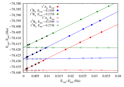
Figure 2: Fit of variational and total energies of ethylene using all data points. The black line is placed at 1.6 mHa. States are separated from one another by 0.01 Ha for clarity. The tightest SHCI calculation used $\epsilon_{\rm V}$ = $7\cdot 10^{-6}$ Ha. The extrapolated energies obtained using all data points are compared to those obtained by omitting the black points in Table 3.

Table 3: Comparison of extrapolated ethylene/ANO-L-pVTZ energies obtained using all the points plotted in Fig. 2 with those obtained from omitting the black points.

State	$E_{\rm extrap}$ (Ha)	$E_{\rm extrap}$ (Ha)
	all points	omit black points
$1^{1}$Ag	-78.4382	-78.4385
$1^{1}$B1u	-78.1424	-78.1430
$1^{3}$B1u	-78.2693	-78.2697

III.3 Ozone

Ozone’s potential energy surfaces have held great interest due to its role in atmospheric chemistry. Andersen2013 An interesting feature predicted by computational studies is the existence of a metastable ring geometry on the ground state surface. Hay1972 A lack of experimental evidence for such a species has fueled multiple studies of the pathway leading to the ring species over the years. Lee1990 ; Qu2005 ; Xantheas1990 ; Xantheas1991 ; Atchity1997 ; Atchity1997a The most recent such study by Ruedenberg et al. utilizes multi-reference CI with up to quadruple excitations, Theis2016 expending considerable effort on selecting and justifying an active space. To provide an accurate picture at critical points along the theorized pathway with even treatment of all valence electrons, SHCI is applied to ozone’s $2^{1}{\rm A}_{\rm 1}$-$1^{1}{\rm A}_{\rm 1}$ gap with the cc-pVTZ basis at the three geometries of interest shown in Figure 3: the equilibrium geometry (termed the open ring minimum (OM)), the hypothetical ring minimum (RM), and the transition state (TS) between these two.

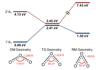
Figure 3: Ozone potential energy surface

As anticipated, sub-mHa perturbative corrections cannot be readily obtained for ozone in the cc-pVTZ basis. $\Delta E_{2}$ for the best available SHCI calculations, at $\epsilon_{\rm V}$=$4\cdot 10^{-5}$ Ha, range from 15-28 mHa for the various geometries and states under consideration. The accuracy of ozone’s extrapolated $2^{1}{\rm A}_{\rm 1}$-$1^{1}{\rm A}_{\rm 1}$ gaps can easily be corroborated for the OM and TS geometries, as the gaps over a broad range of $\epsilon_{\rm V}$’s (Table 4) vary by less than 1 mHa, so the extrapolated values should be even more accurate. The RM geometry’s gap is not as easily corroborated, as these vary over a 2.1 mHa range at reasonably tight $\epsilon_{\rm V}$’s. Therefore, a conservative view would be to take the extrapolated gap as slightly less than chemically accurate.

In Table 5, the SHCI energy gaps are compared to Ruedenberg et al’s MRCI results. Theis2016 SHCI results mostly resemble the MRCI estimates, except for the RM geometry, where the gaps differ by more than 1 eV. The SHCI results, however, are sufficiently converged to allow valuable insights to be made into the meta-stable nature of the RM species. Along the $1^{1}{\rm A}_{\rm 1}$ potential surface, the RM and TS geometries lie 1.30 eV and 2.41 eV, respectively, above the OM geometry. These values suggest that electronic excitations in ozone are likely required to reach RM, but that the RM species should be relatively stable with a 1.11 eV barrier hindering return to the OM geometry. Thus, SHCI indicates that a RM species may well exist, and that experimental investigations should be able to observe it if a plausible isomerization pathway can be accessed.

Table 4: Evolution of ozone $2^{1}{\rm A}_{\rm 1}$ - $1^{1}{\rm A}_{\rm 1}$ gaps (Ha). The RM energy at $\epsilon_{\rm V}=2\cdot 10^{-4}$ is omitted from the fit.

$\epsilon_{\rm V}$	OM	TS	RM
$2\cdot 10^{-4}$	0.1520	0.0009	0.2897
$1\cdot 10^{-4}$	0.1522	0.0008	0.2314
$5\cdot 10^{-5}$	0.1521	0.0005	0.2298
$4\cdot 10^{-5}$	0.1521	0.0006	0.2293
Extrapolated	0.1519	0.0003	0.2254

Table 5: Ozone $2^{1}{\rm A}_{\rm 1}$ - $1^{1}{\rm A}_{\rm 1}$ gaps (eV)

Geometry	Extrapolated SHCI	MRCI (SDTQ)a
OM	4.13	3.54-4.63
TS	0.01	0.05-0.16
RM	6.13	7.35-8.44

• Reference 58

III.4 Shorter Polyenes: Butadiene and Hexatriene

Butadiene and hexatriene are part of the polyene series, long studied for their role as prototypical organic conducting polymers. In particular, the spacing of the low-lying valence excited states has proven especially challenging for electronic structure methods. Tavan1987 ; Watts1996 ; Starcke2006 ; Li1999 ; Nakayama1998 ; Mazur2009 ; Schmidt2012 ; Schreiber2008 ; Piecuch2015 Butadiene and hexatriene are of special interest because their $1^{1}{\rm B}_{\rm 1u}$ and $2^{1}{\rm A}_{\rm g}$ states are nearly degenerate, resulting in conflicting reports of state ordering at lower levels of theory. In the ANO-L-pVDZ basis, butadiene and hexatriene’s FCI spaces of $10^{26}$ and $10^{38}$ determinants, respectively, are too large for the routine application of FCI-level methods, although limited FCIQMC Daday2012 and DMRG Olivares-Amaya2015 studies as well as SHCI ground state calculations HolUmrSha-JCP-17 have been performed on butadiene. Herein, SHCI is applied to the $1^{1}{\rm A}_{\rm g}$, $1^{1}{\rm B}_{\rm 1u}$, $1^{3}{\rm B}_{\rm 1u}$, and $2^{1}{\rm A}_{\rm g}$ states to provide accurate benchmarks and state orderings.

III.4.1 Butadiene

Similar to ozone, extrapolation is used to obtain FCI energy estimates for butadiene in the ANO-L-pVDZ basis, as the tightest SHCI calculations at $\epsilon_{\rm V}$ = $3\cdot 10^{-5}$ Ha had perturbative corrections ranging from 12-29 mHa (Figure 4). Besides using orbitals that minimize the SHCI variational energy, for molecules with more than a few atoms a further improvement in the energy convergence can be obtained by localizing the orbitals. Butadiene has C_2h symmetry, but the localized orbitals transform as the irreducible representations of the C_s subgroup of C_2h. Both the A_g and the B_u irreducible representations of C_2h transform as the A” representation of C_s. Hence calculating the three singlet states, $1^{1}{\rm A}_{\rm g}$, $2^{1}{\rm A}_{\rm g}$ and $1^{1}{\rm B}_{\rm 1u}$ would require calculating three states simultaneously if localized orbitals are used, and further we would not know if the $2^{1}{\rm A}_{\rm g}$ or the $1^{1}{\rm B}_{\rm 1u}$ is lower in energy. Consequently, we calculated only the $1^{1}{\rm A}_{\rm g}$ and $1^{3}{\rm B}_{\rm 1u}$ orbitals using localized orbitals and computed the $2^{1}{\rm A}_{\rm g}$ and $1^{1}{\rm B}_{\rm 1u}$ states with extended orbitals.

Table 6 shows that using the same geometry as in prior FCIQMC, Daday2012 DMRG, Olivares-Amaya2015 and iFCI Zimmerman2017b calculations leads to a SHCI $1^{1}{\rm A}_{\rm g}$ energy that is 0.4 and 0.9 mHa below the extrapolated DMRG extrap_Butadiene_DMRG and iFCI energies respectively. Although FCIQMC has yielded very accurate energies for many systems, in the case of butadiene all three methods (SHCI, iFCI, and DMRG) are in agreement that the FCIQMC energy for the $1^{1}{\rm A}_{\rm g}$ is 8-9 mHa too high. This may be either because of FCIQMC initiator bias or because of an underestimate of the FCIQMC statistical error because of the very long auto-correlation times encountered for large systems. A similar conclusion can be reached for the FCIQMC $1^{1}{\rm B}_{\rm 1u}$ calculation, as the SHCI energy falls below it by a large amount, 12 mHa.

Turning to relative energies, we see that SHCI is in close agreement with all prior FCI-level theoretical calculations. Both the $1^{3}{\rm B}_{\rm u}$-$1^{1}{\rm A}_{\rm g}$ and $1^{1}{\rm B}_{\rm u}$-$1^{1}{\rm A}_{\rm g}$ gaps are 0.08 eV away from the iFCI and FCIQMC values respectively. Although the $2^{1}{\rm A}_{\rm g}$-$1^{1}{\rm A}_{\rm g}$ gap does not currently have FCI-level benchmarks, the agreement of SHCI’s other relative energies with existing benchmarks supports the accuracy of the extrapolated SHCI value for this gap, which is 6.58 eV. This places the $2^{1}{\rm A}_{\rm g}$ state above $1^{1}{\rm B}_{\rm u}$ in butadiene by 0.13 eV. This small gap is consistent with recent theoretical Komainda2017 and experimental Fuss2001 investigations demonstrating ultrafast population transfer from $1^{1}{\rm B}_{\rm u}$ to $2^{1}{\rm A}_{\rm g}$, which implies close proximity of the two states. As with ethylene, relative energies only qualitatively agree with experiment, supporting prior indications that experimental band maxima of butadiene do not correspond to the vertical excitation energy. Watson2012

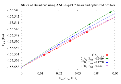
Figure 4: Extrapolation of butadiene SHCI energies. States shifted to extrapolate to the same energy. The tightest SHCI calculation used $\epsilon_{\rm V}$ = $3\cdot 10^{-5}$ Ha.

Table 6: Butadiene total (Ha) and relative energies (eV). Extrapolation errors may range from a few tenths of a mHa for $1^{1}{\rm A}_{\rm g}$ to a couple of mHa for $2^{1}{\rm A}_{\rm g}$.

State	Extrapolated SHCI	FCIQMCa	DMRGb
$1^{1}$Ag	-155.5582(1)	-155.5491(4)	-155.5578
$1^{3}$Bu	-155.4344(1)	-	-
$1^{1}$Bu	-155.3211(1)	-155.3092(6)	-
$2^{1}$Ag	-155.3163(1)	-	-
Gap	Extrapolated SHCI	FCIQMCa	iFCIc	Exp
$2^{1}{\rm A}_{\rm g}$-$1^{1}{\rm A}_{\rm g}$	6.58	-	-	-
$1^{1}{\rm B}_{\rm u}$-$1^{1}{\rm A}_{\rm g}$	6.45	6.53	-	5.92d
$1^{3}{\rm B}_{\rm u}$-$1^{1}{\rm A}_{\rm g}$	3.37	-	3.45	3.22e

• FCIQMC/ANO-L-pVDZ results from reference 71

• DMRG/ANO-L-pVDZ extrapolated energy extrap_Butadiene_DMRG using data from reference 12

• iFCI 6-31G* results from reference 18

• Experimental band maxima from references 102; 103; 104

• Experimental band maxima from reference 105

III.4.2 Hexatriene

Hexatriene is at the current frontier of FCI-level computations, with a demanding FCI space of $10^{38}$ determinants in the ANO-L-pVDZ basis. Only one other algorithm, iFCI, Zimmerman2017a has approached FCI energies for such a large polyatomic - and then only for its singlet-triplet gap. Here we compute the energies of the lowest three singlet states and the lowest triplet state, using values of $\epsilon_{\rm V}$ as small as $2\cdot 10^{-5}$ Ha (Figure 5), which results in as many as $9\cdot 10^{7}$ variational determinants.

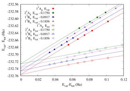
Figure 5: Extrapolation of hexatriene SHCI energies. States are separated from each other by 0.01 Ha for clarity. The tightest SHCI calculation used $\epsilon_{\rm V}$ = $2\cdot 10^{-5}$ Ha.

The extrapolated hexatriene energies are reported in Table 7. With the same geometry, SHCI produces a $1^{1}{\rm A}_{\rm g}$ total energy 4 mHa below iFCI. This difference is within the extrapolation uncertainty of SHCI for this system. Prior investigations of hexatriene photo dynamics Hayden1995 ; Cyr1996 ; Ohta1998 place $1^{1}{\rm B}_{\rm u}$ close in energy to $2^{1}{\rm A}_{\rm g}$. At the vertical excitation geometry, SHCI places $2^{1}{\rm A}_{\rm g}$ below $1^{1}{\rm B}_{\rm u}$ with a small gap of only 0.01 eV. The triplet-singlet $1^{3}{\rm B}_{\rm u}$-$1^{1}{\rm A}_{\rm g}$ gaps computed by SHCI and iFCI (using the slightly smaller 6-31G* basis) differ by only 0.04 eV. As in the case of butadiene, the SHCI $1^{1}{\rm B}_{\rm u}$-$1^{1}{\rm A}_{\rm g}$ gap differs significantly from experiment, Komainda2016 indicating that experimental band maxima do not correspond to vertical excitation energies in hexatriene.

Table 7: Hexatriene total (Ha) and relative energies (eV)

State	Extrapolated SHCI		iFCI
$1^{1}$Ag	-232.7567(1)		-232.7527c
$1^{3}$Bu	-232.6548(1)		-
$1^{1}$Bu	-232.5511(1)		-
$2^{1}$Ag	-232.5517(1)		-
Gap	Extrapolated SHCI	CC	iFCI	Exp
$2^{1}{\rm A}_{\rm g}$-$1^{1}{\rm A}_{\rm g}$	5.58	5.72a	-	5.21e
$1^{1}{\rm B}_{\rm u}$-$1^{1}{\rm A}_{\rm g}$	5.59	5.30a	-	4.95e,5.13e
$1^{3}{\rm B}_{\rm u}$-$1^{1}{\rm A}_{\rm g}$	2.77	2.80b	2.81d	2.61f

• CR-EOMCC(2,3)D/TZVP from reference 67

• CCSD(T)/6-31G* from reference 18

• iFCI/ANO-L-pVDZ result from reference 19

• iFCI/6-31G* result from reference 18

• Raman scattering results from reference 110

• Electron impact band maximum from reference 111

IV Conclusion

SHCI represents an important step forward for SCI methods, providing FCI-quality energies in the largest molecular systems to date. SHCI easily correlates systems of 12 electrons in a triple-zeta basis and can reach FCI-level energies in larger systems through extrapolation. In this paper, CI spaces of $10^{7}-10^{8}$ determinants were used to effectively handle FCI spaces of $10^{26}$ and $10^{38}$ determinants.

This work has provided new benchmarks and insights for the valence states of some commonly investigated molecular systems. Specifically, high-quality SHCI energetics for ozone give strong evidence that the theorized RM structure has a significant barrier to relaxation, and thus should be observable by experiment. Investigation of butadiene and hexatriene lead to the highest level $2^{1}{\rm A}_{\rm g}$/$1^{1}{\rm B}_{\rm u}$ state-orderings in these systems to date, placing $2^{1}{\rm A}_{\rm g}$ above $1^{1}{\rm B}_{\rm u}$ in butadiene, and minutely below $1^{1}{\rm B}_{\rm u}$ in hexatriene. In short, SHCI has shown itself to be an efficient means of obtaining FCI-level energetics, and we look forward to it providing physical insight into other chemically interesting systems with up to dozens of electrons.

- (1) P. Knowles and N. Handy, Chem. Phys. Lett. 111, 315 (1984).
- (2) J. Olsen, B. O. Roos, P. Jørgensen and H. J. A. Jensen, J. Chem. Phys. 89, 2185 (1988).
- (3) J. Olsen, P. Jørgensen and J. Simons, Chem. Phys. Lett. 169, 463 (1990).
- (4) J. Olsen, O. Christiansen, H. Koch and P. Jørgensen, J. Chem. Phys. 105, 5082 (1996).
- (5) E. Rossi, G. L. Bendazzoli, S. Evangelisti and D. Maynau, Chem. Phys. Lett. 310, 530 (1999).
- (6) A. Dutta and C. D. Sherrill, J. Chem. Phys. 118, 1610 (2003).
- (7) Z. Gan, D. J. Grant, R. J. Harrison and D. A. Dixon, J. Chem. Phys. 125, 124311 (2006).
- (8) S. R. White, Phys. Rev. B 48, 10345 (1993).
- (9) S. R. White and R. L. Martin, J. Chem. Phys. 110, 4127 (1999).
- (10) G. K.-L. Chan and M. Head-Gordon, J. Chem. Phys. 116, 4462 (2002).
- (11) G. K.-L. Chan and S. Sharma, Annu. Rev. Phys. Chem. 62, 465 (2011).
- (12) R. Olivares-Amaya, W. Hu, N. Nakatani, S. Sharma, J. Yang and G. K.-L. Chan, J. Chem. Phys. 142, 034102 (2015).
- (13) G. H. Booth, A. J. W. Thom and A. Alavi, J. Chem. Phys. 131, 054106 (2009).
- (14) D. Cleland, G. H. Booth and A. Alavi, J. Chem. Phys. 132, 041103 (2010).
- (15) F. R. Petruzielo, A. A. Holmes, H. J. Changlani, M. P. Nightingale and C. J. Umrigar, Phys. Rev. Lett. 109, 230201 (2012).
- (16) G. H. Booth, A. Gruneis, G. Kresse and A. Alavi, Nature 493, 365 (2013).
- (17) P. M. Zimmerman, J. Chem. Phys. 146, 104102 (2017).
- (18) P. M. Zimmerman, J. Phys. Chem. A 121, 4712 (2017).
- (19) P. M. Zimmerman, J. Chem. Phys. 146, 224104 (2017).
- (20) B. Huron, J. P. Malrieu and P. Rancurel, J. Chem. Phys. 58, 5745 (1973).
- (21) R. J. Buenker and S. D. Peyerimhoff, Theo. Chim. Acta 39, 217 (1975).
- (22) R. J. Buenker, S. D. Peyerimhoff and W. Butscher, Mol. Phys. 35, 771 (1978).
- (23) S. Evangelisti, J. P. Daudey and J. P. Malrieu, Chem. Phys. 75, 91 (1983).
- (24) R. J. Harrison, J. Chem. Phys. 94, 5021 (1991).
- (25) N. Ben Amor, F. Bessac, S. Hoyau and D. Maynau, J. Chem. Phys. 135, 014101 (2011).
- (26) R. J. Buenker and S. D. Peyerimhoff, Theor. Chim. Acta 35, 33 (1974).
- (27) J. Langlet and P. Gacoin, Theor. Chim. Acta 42, 293 (1976).
- (28) E. Oliveros, M. Riviere, C. Teichteil and J.-P. Malrieu, Chem. Phys. Lett. 57, 220 (1978).
- (29) R. Cimiraglia, J. Chem. Phys 83, 1746 (1985).
- (30) R. Cimiraglia and M. Persico, J. Comp. Chem. 8, 39 (1987).
- (31) P. J. Knowles, Chem. Phys. Lett. 155, 513 (1989).
- (32) R. J. Harrison, J. Chem. Phys. 94, 5021 (1991).
- (33) A. Povill, J. Rubio and F. Illas, Theor. Chim. Acta 82, 229 (1992).
- (34) M. M. Steiner, W. Wenzel, K. G. Wilson and J. W. Wilkins, Chem. Phys. Lett. 231, 263 (1994).
- (35) V. Garcia, O. Castell, R. Caballol and J. Malrieu, Chem. Phys. Lett. 238, 222 (1995).
- (36) W. Wenzel, M. Steiner and K. G. Wilson, Int. J. Quantum Chem. 60, 1325 (1996).
- (37) F. Neese, J. Chem. Phys. 119, 9428 (2003).
- (38) H. Nakatsuji and M. Ehara, J. Chem. Phys. 122, 194108 (2005).
- (39) M. L. Abrams and C. D. Sherrill, Chem. Phys. Lett. 412, 121 (2005).
- (40) L. Bytautas and K. Ruedenberg, Chem. Phys. 356, 64 (2009).
- (41) R. Roth, Phys. Rev. C 79, 064324 (2009).
- (42) F. A. Evangelista, J. Chem. Phys. 140, 054109 (2014).
- (43) P. J. Knowles, Mol. Phys. 113, 1655 (2015).
- (44) J. B. Schriber and F. A. Evangelista, J. Chem. Phys. 144, 161106 (2016).
- (45) W. Liu and M. R. Hoffmann, J. Chem. Theory Comput. 12, 1169 (2016).
- (46) T. Zhang and F. A. Evangelista, J. Chem. Theory Comput. 12, 4326 (2016).
- (47) A. Scemama, T. Applencourt, E. Giner and M. Caffarel, J. Comp. Chem. 37, 1866 (2016).
- (48) Y. Garniron, A. Scemama, P.-F. Loos and M. Caffarel, J. Chem. Phys. 147, 034101 (2017).
- (49) E. Giner, C. Angeli, Y. Garniron, A. Scemama and J.-P. Malrieu, J. Chem. Phys. 146, 224108 (2017).
- (50) J. B. Schriber and F. A. Evangelista, J. Chem. Theory Comput. 13, 5354 (2017).
- (51) A. A. Holmes, N. M. Tubman and C. J. Umrigar, J. Chem. Theory Comput. 12, 3674 (2016).
- (52) S. Sharma, A. A. Holmes, G. Jeanmairet, A. Alavi and C. J. Umrigar, J. Chem. Theory Comput. 13, 1595 (2017).
- (53) A. A. Holmes, C. J. Umrigar and S. Sharma, J. Chem. Phys. 147, 164111 (2017).
- (54) J. E. T. Smith, B. Mussard, A. A. Holmes and S. Sharma, J. Chem. Theory Comput. 13, 5468 (2017).
- (55) B. Mussard and S. Sharma, J. Chem. Theory Comput. 14, 154 (2017).
- (56) C. D. Sherrill, M. L. Leininger, T. J. Van Huis and H. F. Schaefer, J. Chem. Phys. 108, 1040 (1998).
- (57) P. Hay and W. Goodard, Chem. Phys. Lett. 14, 46 (1972).
- (58) D. Theis, J. Ivanic, T. L. Windus and K. Ruedenberg, J. Chem. Phys. 144, 104304 (2016).
- (59) P. Tavan and K. Schulten, Phys. Rev. B 36, 4337 (1987).
- (60) J. D. Watts, S. R. Gwaltney and R. J. Bartlett, J. Chem. Phys. 105, 6979 (1996).
- (61) J. H. Starcke, M. Wormit, J. Schirmer and A. Dreuw, Chem. Phys. 329, 39 (2006).
- (62) X. Li and J. Paldus, Int. J. Quantum Chem. 74, 177 (1999).
- (63) K. Nakayama, H. Nakano and K. Hirao, Int. J. Quantum Chem. 66, 157 (1998).
- (64) M. Schreiber, M. R. Silva-Junior, S. P. A. Sauer and W. Thiel, J. Chem. Phys. 128, 1 (2008).
- (65) G. Mazur and R. Włodarczyk, J. Comput. Chem. 30, 811 (2009).
- (66) M. Schmidt and P. Tavan, J. Chem. Phys. 136, 124309 (2012).
- (67) P. Piecuch, J. A. Hansen and A. O. Ajala, Mol. Phys. 113, 3085 (2015).
- (68) T. H. Dunning, J. Chem. Phys. 90, 1007 (1989).
- (69) R. A. Kendall, T. H. Dunning and R. J. Harrison, J. Chem. Phys. 96, 6796 (1992).
- (70) P.-O. Widmark, P.-Å. Malmqvist and B. O. Roos, Theor. Chim. Acta 77, 291 (1990).
- (71) C. Daday, S. Smart, G. H. Booth, A. Alavi and C. Filippi, J. Chem. Theory Comput. 8, 4441 (2012).
- (72) A. I. Krylov and P. M. W. Gill, Wiley Interdiscip. Rev. Comput. Mol. Sci. 3, 317 (2013).
- (73) M. Włoch, M. D. Lodriguito, P. Piecuch and J. R. Gour, Mol. Phys. 104, 2149 (2006).
- (74) P. U. Manohar and A. I. Krylov, J. Chem. Phys. 129, 194105 (2008).
- (75) H. F. Schaefer, Science 231, 1100 (1986).
- (76) C. W. Bauschlicher and P. R. Taylor, J. Chem. Phys. 85, 6510 (1986).
- (77) C. Sherrill, T. J. Van Huis, Y. Yamaguchi and H. F. Schaefer, J. Mol. Struct. THEOCHEM 400, 139 (1997).
- (78) P. M. Zimmerman, J. Toulouse, Z. Zhang, C. B. Musgrave and C. J. Umrigar, J. Chem. Phys. 131, 124103 (2009).
- (79) L. V. Slipchenko and A. I. Krylov, J. Chem. Phys. 117, 4694 (2002).
- (80) Y. Shao, M. Head-Gordon and A. I. Krylov, J. Chem. Phys. 118, 4807 (2003).
- (81) A. D. Chien and P. M. Zimmerman, Mol. Phys. 116, 107 (2017).
- (82) P. Jensen and P. R. Bunker, J. Chem. Phys. 89, 1327 (1988).
- (83) A. Alijah and G. Duxbury, Mol. Phys. 70, 605 (1990).
- (84) E. R. Davidson, J. Phys. Chem. 100, 6161 (1996).
- (85) T. Müller, M. Dallos and H. Lischka, J. Chem. Phys. 110, 7176 (1999).
- (86) C. Angeli, Int. J. Quantum Chem. 110, 2436 (2010).
- (87) R. S. Mulliken, J. Chem. Phys. 66, 2448 (1977).
- (88) J. H. Moore and J. P. Doering, J. Chem. Phys. 52, 1692 (1970).
- (89) J. H. Moore, J. Phys. Chem. 76, 1130 (1972).
- (90) E. Van Veen, Chem. Phys. Lett. 41, 540 (1976).
- (91) S. O. Andersen, M. L. Halberstadt and N. Borgford-Parnell, J. Air Waste Manage. Assoc. 63, 607 (2013).
- (92) T. J. Lee, Chem. Phys. Lett. 169, 529 (1990).
- (93) Z.-W. Qu, H. Zhu and R. Schinke, J. Chem. Phys. 123, 204324 (2005).
- (94) S. Xantheas, S. T. Elbert and K. Ruedenberg, J. Chem. Phys. 93, 7519 (1990).
- (95) S. S. Xantheas, G. J. Atchity, S. T. Elbert and K. Ruedenberg, J. Chem. Phys. 94, 8054 (1991).
- (96) G. J. Atchity and K. Ruedenberg, Theor. Chim. Acta 96, 176 (1997).
- (97) G. J. Atchity, K. Ruedenberg and A. Nanayakkara, Theor. Chim. Acta 96, 195 (1997).
- (98) An extrapolated value of -155.5578 was obtained by fitting the values in Table VI of Ref. 12 to either a linear or a quadratic function of , where is the DMRG bond dimension.
- (99) A. Komainda, D. Lefrancois, A. Dreuw and H. Köppel, Chem. Phys. 482, 27 (2017).
- (100) W. Fuß, W. Schmid and S. Trushin, Chem. Phys. Lett. 342, 91 (2001).
- (101) M. A. Watson and G. K.-L. Chan, J. Chem. Theory Comput. 8, 4013 (2012).
- (102) O. A. Mosher, W. M. Flicker and A. Kuppermann, J. Chem. Phys. 59, 6502 (1973).
- (103) R. McDiarmid, J. Chem. Phys. 64, 514 (1976).
- (104) J. P. Doering and R. McDiarmid, J. Chem. Phys. 73, 3617 (1980).
- (105) O. A. Mosher, W. M. Flicker and A. Kuppermann, Chem. Phys. Lett. 19, 332 (1973).
- (106) C. C. Hayden and D. W. Chandler, J. Phys. Chem. 99, 7897 (1995).
- (107) D. R. Cyr and C. C. Hayden, J. Chem. Phys. 104, 771 (1996).
- (108) K. Ohta, Y. Naitoh, K. Tominaga, N. Hirota and K. Yoshihara, J. Phys. Chem. A 102, 35 (1998).
- (109) A. Komainda, I. Lyskov, C. M. Marian and H. Köppel, J. Phys. Chem. A 120, 6541 (2016).
- (110) T. Fujii, A. Kamata, M. Shimizu, Y. Adachi and S. Maeda, Chem. Phys. Lett. 115, 369 (1985).
- (111) W. M. Flicker, O. A. Mosher and A. Kuppermann, Chem. Phys. Lett. 45, 492 (1977).