Evidence of energy and charge sign dependence of the recovery time for the December 2006 Forbush event measured by the PAMELA experiment

Abstract

New results on the short-term galactic cosmic ray (GCR) intensity variation (Forbish decrease) in December $2006$ measured by the PAMELA instrument are presented. Forbush decreases are sudden suppressions of the GCR intensities which are associated with the passage of interplanetary transients such as shocks and interplanetary coronal mass ejections (ICMEs). Most of the past measurements of this phenomenon were carried out with ground-based detectors such as neutron monitors or muon telescopes. These techniques allow only the indirect detection of the overall GCR intensity over an integrated energy range. For the first time, thanks to the unique features of the PAMELA magnetic spectrometer, the Forbush decrease commencing on $2006$ December 14, following a CME at the Sun on $2006$ December $13$ was studied in a wide rigidity range ($0.4-20$ GV) and for different species of GCRs detected directly in space. The daily averaged GCR proton intensity was used to investigate the rigidity dependence of the amplitude and the recovery time of the Forbush decrease. Additionally, for the first time, the temporal variations in the helium and electron intensities during a Forbush decrease were studied. Interestingly, the temporal evolutions of the helium and proton intensities during the Forbush decrease were found in good agreement, while the low rigidity electrons ($<2$ GV) displayed a faster recovery. This difference in the electron recovery is interpreted as a charge-sign dependence introduced by drift motions experienced by the GCRs during their propagation through the heliosphere.

1 Introduction

The solar environment significantly affects the spectrum of galactic cosmic rays (GCRs) observed at Earth below a few tens of GV. Before reaching the Earth, GCRs propagate through the heliosphere, the region of space formed by the continuous outflow of plasma from the solar corona, also known as the solar wind (SW). In addition, the magnetic field of the Sun freezes into the solar wind plasma and is transported through the heliosphere, forming the so called heliospheric magnetic field (HMF) (Parker, 1963). The GCRs, traveling through the interplanetary medium, interact with the SW and the HMF. As a consequence their spectra are modified in intensity and shape with respect to the local interstellar spectrum (LIS) (Potgieter, 2013). In addition, in response to the $11$-years solar cycle (Hathaway, 2015), a long-term modulation of the GCRs is observed. The solar modulation of GCR is anti-correlated with respect to the solar cycle since the particle fluxes reach their maximal intensity during periods of low solar activity.

On top of the long-term solar modulation, short-term modulation effects also occur. For example, the GCR intensity may be modulated by transient phenomena as interplanetary coronal mass ejections (e.g. Barnden (1976); Richardson et al. (2011) and references therein). These ICMEs consist of magnetized coronal plasma ejected from the Sun’s surface that then propagates through the heliosphere. Some ICMEs propagate through the solar wind at super-Alfvenic speeds and drive a shock ahead of them (e.g. Jian et al. (2006)). As the ICME passes near Earth the sheath following the shock acts as a shield against the ambient population of GCRs since they cannot easily diffuse through the region of enhanced turbulence in the sheath (Wibberenz et al., 1997). Moreover, as it propagates from the Sun to the Earth, the ICME itself is progressively populated by GCRs that perpendicularly diffuse into the magnetic cloud (e.g. Cane et al. (1995); Arunbabu et al. (2013); Krittinatham et al. (2009); Kubo et al. (2010)). As an overall effect a sudden suppression of GCR intensity is observed. Such a phenomenon initially identified by Forbush (1937) (and also by Hess and Demmelmair (1937)) and hence called a Forbush decrease, can last up to several days suppressing the GCR intensity up to about $30\%-40\%$ or even more (e.g. Cane (2000) and references therein). The relative contributions of shocks and ICMEs in causing Forbush decreases is still a matter of debate, and likely varies from event to event and observationally depends on the trajectory of the observer through the shock and ICME (e.g., Figure 1 of Richardson et al. (2011)). In addition, recurrent short-term GCR decreases have been measured in association with the passage of corotating interaction regions (CIRs). Such regions of compressed plasma, formed at the leading edges of high-speed solar wind streams originating from coronal holes and interacting with the preceding slow solar wind, are a well known cause of periodic CR decreases (e.g. Simpson (1998); Richardson (2004) and references therein). The study of the CIR associated GCR intensity decreases with the PAMELA data will be the subject of a future paper.

The Forbush decrease, observed by the PAMELA space mission discussed in this work, occurred in December 2006, during the extraordinary deep and prolonged solar minimum between solar cycles 23 and 24 (Potgieter et al., 2014; Russell et al., 2010). Solar minimum periods are particularly interesting to measured transient phenomena like Forbush decrease. Being the Sun’s activity at minimum, the overall structure of the HMF is well ordered and easier to reproduce from a modeling point of view. Moreover the time variation of GCR intensity is slower with respect to a period of high Sun’s activity. Solar minima are thus well suited to study and disentangle the relative contribution to the GCR intensity variations due to ICME and shocks from that due to solar modulation. Remarkably, the minimum between solar cycles 23 and 24 was characterized by very stable heliospheric conditions, except for the powerful solar events that occurred during December $2006$. Four X class solar flares originated during December $2006$ as solar active region $10930$ rotated across the visible hemisphere of the Sun. The first of these X-class flares (X$9.0$) occurred on $2006$ December $5$ at E$79$° with peak emission at $1035$ UT and was followed by an X$6.5$ flare on the $2006$ December $6$ at E$63$°, with peak emission at $1847$ UT. On the $2006$ December $13$ another X$3.4$ flare occurred at W$23$° with peak emission at $0240$ UT followed by a X$1.5$ flare on the $2006$ December $14$ at W$46$°  with peak emission at $2215$ UT (von Rosenvinge et al., 2009). These events produced an enhancement of particles up to several GV that was recorded and extensively studied by the PAMELA instrument (Adriani et al., 2011a) and other satellites. The PAMELA instrument also measured the variations of the geomagnetic cutoff latitude as a function of rigidity during the $2006$ December $14$ magnetospheric storm caused by the ICME associated with the December $13$ event (Adriani et al., 2016a). Figure 1 shows the proton intensity ($400$-$1000$ MV) measured in December $2006$ by the PAMELA instrument (full circles). Data are normalized to the November $2006$ average proton intensity that was considered as the GCR background level. Each point represents three hours of data taking. For comparison the GOES-12 proton integrated data ($>310$ MV) are shown (full squares). The GOES-12 data were also normalized to the November $2006$ average proton intensity. The PAMELA data exhibit a sudden increase in the proton intensity associated with the X3.4 flare on 13 December. However, due to a scheduled maintenance procedure, no data were collected during the 5/6 December events. The GOES-12 data show an increase of the proton intensity corresponding to all four of the X-class flares in December $2006$. In addition, halo CMEs were observed by the LASCO coronagraphs on SOHO in association with the events of $2006$ December 13 and 14, with speeds of $1774$ km/s and $1042$ km/s $($data taken from https://cdaw.gsfc.nasa.gov/CME_list/$)$ respectively while the $2006$ December 5 and 6 events occurred during SOHO/LASCO data gaps.

The passage of the $2006$ December $13$ CME caused a Forbush decrease that lasted for several days which is evident in Figure 1 and will be shown in greater detail below. Thanks to its quasi-polar orbit the PAMELA instrument has measured this event in the rigidity range from $400$ MV to $20$ GV. This extends and completes studies based on other measurements, typically performed on the ground, either by neutron monitors or muon telescopes (e.g. Vieira et al. (2012); Usoskin et al. (2008)). The performance of these ground-based detectors is limited since they can only determine an integral flux above an energy threshold that depends on the latitudinal geomagnetic cutoff at the location of the monitor. For the first time a Forbush decrease was extensively studied with GCRs detected directly in space in a wide rigidity range. The accuracy of the rigidity reconstruction and the high counting statistics allowed the rigidity-dependences of the amplitude and the recovery time of this event to be studied. In addition, the PAMELA instrument allowed the temporal evolution of the GCRs to be studied for several particle species. In particular the galactic cosmic ray proton, helium and electron intensities over time were studied. By comparing GCRs with oppositely signed charges, it is possible to identify differences in the Forbush decrease amplitude and recovery time that could be introduced by drift motions experienced by the GCRs during their interaction with and propagation through the ICME (Luo et al., 2017). After a brief discussion of the PAMELA instrument in Section 2 the data analysis will be discussed in Section 3 and the results will be presented in Section 4.

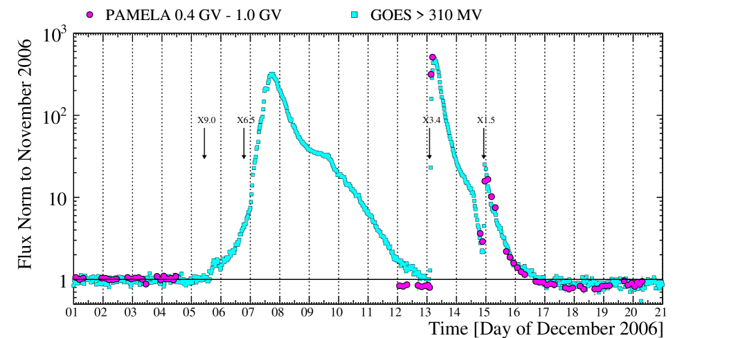
Figure 1: The PAMELA proton intensity (full circles) measured between the $2006$ December 1 and 21 in the rigidity range $0.4$ - $1.0$ GV. The horizontal line represents the GCR reference intensity to which the data were normalized, i.e. the average intensity of GCRs proton measured during November $2006$. Each point represents three hours of data taking. Missing data are due to maintenance procedure and on-board system reset of the satellite. The integrated GOES-12 proton data $>310$ MV (full squares) averaged over $30$ minutes are also showed for comparison. Data were taken from http://satdat.ngdc.noaa.gov/sem/goes/data/new_full and were normalized to the average November $2006$ GOES-12 proton intensity. PAMELA and GOES-12 data show the $2006$ December 13 and 14 SEP events registered as a sudden increase of the proton intensity. GOES-12 data also shows the $2006$ December 5 and 6 event. The flare time at the Sun is indicating by the vertical arrows.

2 The PAMELA instrument

PAMELA, Payload for Antimatter-Matter Exploration and Light-nuclei Astrophysics, is a satellite-borne experiment designed to make long duration measurements of the cosmic radiation from Earth orbit (Picozza et al., 2007). The instrument collected GCRs in space for almost ten years from the $2006$ June $15$ when it was launched from the Baikonur cosmodrome in Kazakhstan, to late January $2016$. Until September $2010$ the orbit was elliptical with altitudes ranging between $350$ and $610$ km with an inclination of $70$ degrees. After $2010$ the orbit was changed and became circular at a constant altitude of $570$ km.

The apparatus is schematically shown in Figure 2. The core of the instrument is the magnetic spectrometer (Adriani et al., 2003), a silicon tracking system in the $0.43$ T magnetic field generated by a permanent magnet. The $300\;\mu$m thick double-sided Si sensors of the tracking system measure two independent impact coordinates (bending X-view and non-bending Y-view) on each plane, accurately reconstructing the particle deflection, measuring its rigidity (momentum divided by charge) with a maximum detectable rigidity of $1.2$ TV, and the sign of the electric charge. The instrument geometric factor, as defined by the magnetic cavity, is $21.5$ cm² sr. A system of six layers of plastic scintillators, arranged in three double planes (S1, S2 and S3), provides a fast signal for triggering the data acquisition. Moreover it contributes to particle identification measuring the ionization energy loss and the Time of Flight (ToF) of traversing particles with a resolution of $300$ ps, assuring charge particle absolute value determination and albedo particle rejection (Osteria et al., 2004). The hadron-lepton discrimination is provided by an electromagnetic imaging W/Si calorimeter, $16.3$ radiation lengths and $0.6$ interaction lengths deep (Boezio et al., 2002). Thanks to its longitudinal and transverse segmentation, the calorimeter exploits the different development of electromagnetic and hadronic showers, allowing a rejection power of interacting and non-interacting hadrons at the order of $10^{5}$. A neutron counter (Stozhkov et al., 2005) contributes to discrimination power by detecting the increased neutron production in the calorimeter associated with hadronic showers compared to electromagnetic ones, while a plastic scintillator, placed beneath the calorimeter, increases the identification of high-energy electrons. The whole instrument is surrounded by an anticoindence system (AC) of three scintillators (CARD, CAS and CAT) for the rejection of background events (Orsi et al., 2005). For a complete review of the PAMELA apparatus see (Adriani et al., 2014, 2017).

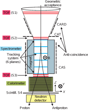
Figure 2: PAMELA and its sub-detectors.

3 Data analysis

A set of criteria based on the information provided by the sub-detectors described in the previous section was developed in order to select a clean sample of protons, helium and electrons from the data collected by the PAMELA instrument. Only events with a single reconstructed track were selected. The track was required to be located inside a fiducial volume bounded $0.15$ cm from the magnet cavity walls in order to avoid interaction with the magnetic walls which could degrade the tracker performance. Protons and helium nuclei were selected by means of the ionization energy losses in the tracker and the ToF planes. Figure 3 (left panel) shows the average ionization energy loss in terms of minimum ionizing particle (MIP) inside the silicon tracker planes. Data were collected by the PAMELA instrument between July and December $2006$. The black lines represent a constant efficiency selections on the proton (lower bands) and helium (upper bands) nuclei. No isotopic separation (proton/deuterium or ³He/⁴He) was performed in this analysis. The dE/dx selections provide a clean sample of helium nuclei and a sample of protons with a negligible positron contamination of the order of $10^{-4}$-$10^{-5}$ over the whole energy range. For more detail about the proton and the helium selection see (Adriani et al., 2011b).

Electrons were selected exploiting the PAMELA electromagnetic calorimeter. The main background is represented by galactic antiprotons (a few percent of the signal) and negative pions which are produced by the interaction of primary cosmic rays nuclei with the aluminum container that encloses the PAMELA instrument (few percent below $\sim$ 5 GV). Several selections based on the topological development of the particle shower were defined. Figure 3 (right panel) shows the rigidity distribution of one calorimetric variable which was defined in order to emphasize the multiplication and the collimation of the electromagnetic shower. This variable represents the sum over all the calorimeter planes of the number of strip hit around a few centimeters from the shower axis. Since the leptonic shower is more collimated than the hadronic one, electrons are characterized by higher values of this variable as shown in Figure 3. The black lines represent a constant efficiency selection defined in order to reject antiproton and negative pion contamination. A set of six calorimetric selections allowed an almost complete rejection of the antiproton and pion contamination in the rigidity range considered. The residual contamination was estimated using both simulated and flight data and was found to be less than one percent over the whole energy range. For more details about the electron selections and the estimation of the residual contamination see (Adriani et al., 2015).

In order to reject reentrant albedo particles, the events were selected by imposing that the lower edge of the rigidity bin to which the event belongs exceeds the critical rigidity, defined as $1.3$ times the geomagnetic cutoff rigidity computed in the Störmer vertical approximation (Shea et al., 1987)

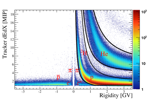
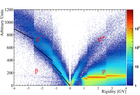
Figure 3: Left panel: the average ionization energy losses on the tracker planes as a function of the rigidity measured by the magnetic spectrometer. The helium, proton, electron and pion distributions are well separated thanks to the excellent MIP resolution. The upper and the lower bands (bounded black lines) represent the selections for the helium nuclei and protons respectively. Right panel: a calorimetric variable as a function of the particles rigidity. The black lines represent a constant efficiency selection defined in order to separate the hadronic and leptonic signals.

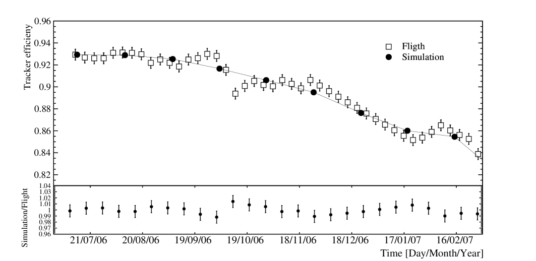
Figure 4: Top panel: the efficiency of the tracker selection as a function of time. The open squares represent the weekly efficiency evaluated with flight data while the full circles represents the simulated efficiency averaged on one month. The solid line connecting the simulated efficiencies represents the final values used for the flux calculation. Bottom panel: the ratio between the simulated and flight efficiencies. The ratio was calculated interpolating the simulated efficiencies for the temporal division of the flight efficiency.

The proton, helium and electron fluxes were finally calculated by dividing the number of particles by the selection efficiencies, the live-time and the geometrical factor. To avoid any biases which could introduce systematic temporal variation in the fluxes, the temporal evolution of the selection efficiencies was studied. The dE/dx selection was found to have constant efficiencies during the whole time interval under analysis. Also the calorimeter selection efficiencies were found constant over time. On the contrary the tracker selection efficiency was found to decrease over time. This effect is ascribed to the random failure of few read-out chips of the silicon mictrostrip detectors. The tracker efficiency was evaluated with two independent procedures over the period of time from the beginning of data taking until May 2007:

• The PAMELA simulation software (based on GEANT4 (Agostinelli et al., 2003)) was used to generate an isotropic set of protons in the energy range under analysis. The events reconstructed inside the instrumental acceptance were used to measure the energy dependence of the tracker efficiency. The simulation toolkit reproduced the flight configuration of the tracker planes and its temporal evolution. Because of the huge computational time required to process all the different tracker configurations, the simulated efficiency was evaluated with a temporal resolution of one month.

• Non-interactive protons that do not produce a hadronic shower in the calorimenter and release energy only along their track were selected with the calorimeter from flight data. These events were used to measure the tracker selection efficiency. This procedure allows the efficiency to be estimated only within an integrated energy range with a lower threshold of few GeV. The high statistics allowed to estimate the weekly integrated efficiency during the period of time under analysis.

The results are displayed in Figure 4 (top panel) where both the simulated (full circles) and the flight (open squares) tracker efficiency as a function of time are shown. As can be noticed from the bottom panel of Figure 4 an agreement of the order of $2-3\%$ was found between the simulated and the flight efficiencies over the whole time interval. Because of the good agreement between the simulated and the flight efficiencies, in order to minimize the statistical fluctuation, the final fluxes were calculated using the interpolated values of the simulated efficiencies, i.e. the solid line connecting the simulated efficiencies in Figure 4. The differences between the simulated and the flight efficiencies were considered as a systematical uncertainties associated to the flux evaluation.

The geometrical acceptance, i.e. the requirement of triggering and containment, at least $1.5$ mm away from the magnet walls and the TOF-scintillator edge, was evaluated by simulating an isotropic flux of particles over the PAMELA detector. A constant value of $19.9$ cm² sr was found above $\sim 1$ GV decreasing at low energy due to the increasing particle bending. The live time was provided by an on-board clock that timed the periods during which the apparatus was waiting for a trigger. Because of the relatively short time spent by the satellite at high geomagnetic latitudes, the total live time, and thus the collected statistics, was reduced to about $10\%$ of the total value at $500$ MV.

In order to study the temporal variation of the GCR flux during December $2006$ the particle intensities were normalized to the averaged flux measured during the calendar month before the event, i.e. November $2006$. A constant linear fit was performed to the proton, helium and electron fluxes between the $2006$ November 1 and 30. Then the fluxes were normalized to these values. It was assumed that for the duration of the Forbush event, changes due to the long-term solar modulation had a negligible effect on the GCR intensity.

The Forbush decrease amplitude and recovery time were studied with protons in nine rigidity intervals between $0.4$ and $20$ GV. The statistics allowed the proton flux to be measured with a time resolution of $3$ or $6$ hours up to $5$ GV and with a time resolution of one day above $5$ GV. Because of the limited statistics with respect to protons, the helium and electron fluxes were evaluated with a two days time resolution.

4 Results

4.1 Intensity time profile

Figure 5 places the proton intensity-time profile measured by the PAMELA instrument and the neutron intensity measured by the Oulu neutron monitor in the context of near-Earth solar wind observations. In detail, the bottom panel of Figure 5 shows the proton intensity between $3$ and $4$ GV (full circles) measured by the PAMELA spectrometer with three hours temporal resolution compared with the hourly averaged neutron intensity measured by the Oulu neutron monitor (full squares). The PAMELA and the Oulu data are normalized to the average November $2006$ intensity. The other panels of Figure 5 show from the top: the magnetic field intensity (panel a), the azimuthal angle in GSE coordinates (panel b), the solar wind proton temperature (panel c), speed (panel d) and density (panel e). Panel (f) shows the solar wind ion charge state observation from the SWICS instrument on ACE, specifically, the O⁷/O⁶ ratio.

As already pointed out in Section 1, neutron monitors respond to the GCR intensity variation over an integrated rigidity range with a lower threshold defined by their position on the Earth’s surface. The lower threshold for the Oulu neutron monitor is about $0.8$ GV. Moreover, neutron monitors are fixed on the Earth’s surface while an instrument like PAMELA continuously orbits around the Earth. For these reasons the finer scale Oulu and PAMELA intensity variations during the Forbush decrease cannot be directly compared. Nevertheless, Figure 5 represents a useful crosscheck of the time evolution of the event. Moreover, the Oulu neutron monitor intensity fills in the gaps when PAMELA data are missing.

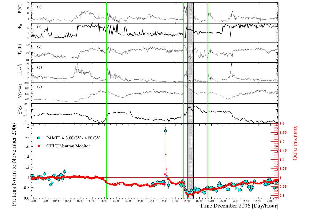
Figure 5: From the top: the HMF intensity (panel a), the HMF azimuthal angles in GSE coordinates (panel b), the solar wind proton temperature (panel c), speed (panel d) and density (panel e) for $2006$ December $2$-$22$. Data are all $5$ minutes averages from the OMNI database (https://omniweb.gsfc.nasa.gov/). Panel (f) shows the solar wind ion charge state observation from the SWICS instrument on ACE, specifically, the O⁷/O⁶ ratio. Bottom panel: the three hours time resolution proton intensity measured between $3$ and $4$ GV with the PAMELA instrument (full circles) compared with the Oulu neutron monitor intensity averaged over one hour (full squares). The solid horizontal line represents the reference intensity on which data were normalized (November $2006$). Solid lines connecting the neutron monitor intensity are displayed only to guide the eye. Vertical lines indicate times of shock passage while the grey shaded region indicates the passage of a magnetic cloud.

From Figure 5 it can be noticed that the solar events of the $2006$ December $5$ and $6$ already produced a decrease in the GCR intensity that started at about the $1200$ UT of the $2006$ December $7$. The GCR decrease on December $7$ commenced just ahead of the arrival of a weak shock indicated by the first vertical line (the shock identification is from the shock database maintained by the University of Helsinki http://ipshocks.fi/). Since the GCR decrease clearly starts ahead of shock arrival, it is possible that the initial decrease could be associated with the corotating high speed stream through which the shock was propagating (see e.g. Cane et al. (1993); Thomas et al. (2005)). The extended GCR decrease without a recovery may then be associated with the persistent high speed flows that continue beyond the time of the ground level event on $2006$ December $13$ in the Oulu data. This suppression in the GCR intensity is also evident when the PAMELA data resume on $2006$ December $12$, with a decrease of about $10\%$ with respect to the average November GCR intensity, and continues to be present after the temporary increase associated with the $2006$ December $13$ solar event.

The abrupt GCR decrease on December 14 commenced immediately following passage of the shock related to the solar event on $2006$ December 13. The shock (second vertical line) produced a geomagnetic storm sudden commencement at 1414 UT when it reached Earth (times from the CfA shock database, https://www.cfa.harvard.edu/shocks/). Signatures typical of ICMEs are evident for around four days following the shock, including intervals of depressed solar wind proton temperatures (panel c) and enhanced solar wind ion charge states (panel f). Following the shock on December 14, the GCR intensity declined and reached a minimum in the ICME with a magnetic cloud structure (Klein and Burlaga, 1982) present on $2006$ December $15$ (gray shaded band). This shock and the ICME-associated structures immediately following are discussed in more detail by e.g. Liu et al. (2008); Richardson and Cane (2010). At least one other shock passed by during this period of ICME-associated structures (third vertical line), observed by Wind (at 1734 UT) and ACE (1721 UT) on December 16. The complexity of these structures indicates that this region is formed by the interaction of multiple ICMEs but further analysis of these structures is beyond the scope of this paper.

The observations suggest that the decrease commenced on the $2006$ December $13$ then added to the larger decrease commencing on December 14, though the contributions of the two decreases cannot be disentangled. Therefore, in this study the decrease commencing on December 14 is treated here as being entirely due to the passage of the shock and ICME on December $14$-$15$.

Figure 6 shows the proton intensity-time profile measured by the PAMELA instrument (three hour time resolution) over three different rigidity intervals. The intensity profile measured at the lowest rigidity ($0.4$-$1$ GV) shows the arrival of the solar energetic particles around $0300$ UT on the $2006$ December $13$ and again around $2200$ UT on the $2006$ December 14 associated with the flares and fast CMEs at these times described above. Missing data are due to on-board system reset caused by the high trigger rate that occurred during the solar events. Solar energetic particles between $0.4$ and $2$ GV were visible following both solar events, while between $2$ - $3$ GV, only the $2006$ December 13 solar event produced a visible increase. Above $1$ GV the Forbush decrease started around $1200$ to $1500$ UT on the $2006$ December $14$, associated with the arrival of the interplanetary shock and reached the minimum intensity during the first half of $2006$ December $15$ at $2$-$3$ GV, $1$-$2$ GV protons being dominated by solar particles at this time.

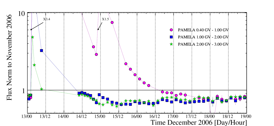
Figure 6: The three hour time resolution proton intensity measured with the PAMELA instrument. Three different rigidity intervals are displayed between the $2006$ December $13$ and $18$. The solid horizontal line represents the reference intensity to which the data were normalized, i.e. the average GCR intensity measured during November $2006$ by PAMELA. Solid lines connecting each point are displayed only to guide the eye. The arrows indicate the time of the flares at the Sun.

Below 1 GV, solar energetic particles continue to dominate, and the intensity only falls below the pre-event background, indicating a decrease in the GCR intensity, approximatively three days later at around $2100$ UT on the $2006$ December $16$ and reached its minimum intensity around $0000$ UT on the $2006$ December $18$.

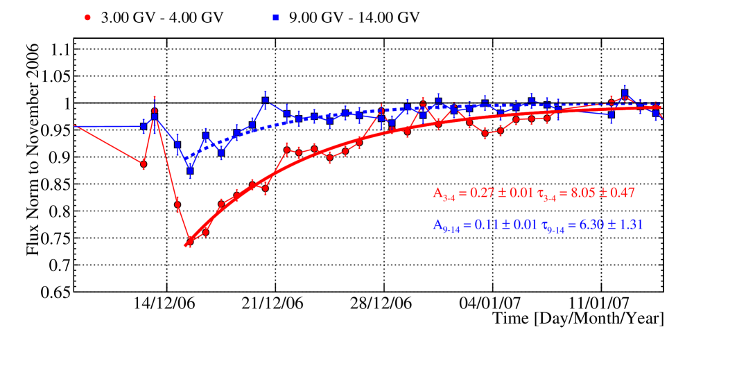
Figure 7: The proton intensity over time measured by the PAMELA instrument between $2006$ December $14$ and $2007$ January $16$. Each point represents one day of data taking. Two rigidity intervals are showed: 3-4 GV (circle points) and 9-14 GV (square points). The solid and the dotted lines represent a fit performed with Equation 1 to the 3-4 GV and 9-14 GV interval respectively. The values for the amplitude $A$ and the recovery time $\tau$ obtained from the fit are also showed.

4.2 Amplitude and recovery time rigidity dependence

The amplitude and the recovery time of the Forbush decrease commencing on $2006$ December $14$ was studied by fitting the time profile of the daily average proton fluxes, $I(t)$, in nine different rigidity intervals. The following function was used (e.g. Jämsén et al. (2007); Usoskin et al. (2008)):

$$I(t)=1-A\ e^{-\frac{t-t_{0}}{\tau}}$$ (1)

The free parameters are the amplitude $A$ of the decrease with respect to the reference flux and the recovery time $\tau$. The absolute reference time $t_{0}$, which represent the starting time of the Forbush decrease, is fixed. Both $\tau$ and $t_{0}$ are expressed in days. As already discussed in Section 4.1, because of the prolonged presence of the solar particles, between $0.4$ and $1$ GV the Forbush decrease (measured by the PAMELA instrument) starts with three days of delay with respect to the higher rigidities. For this reason above $1$ GV the fit was performed between the $2006$ December $15$ at $0000$ UT and the $2007$ January $31$ at $2400$ UT while below $1$ GV the fit was performed starting from the $2006$ December $18$ at $0000$ UT. However, by assuming that the Forbush decrease started at the same time for all the rigidities, the amplitude and the recovery time below 1 GV were also calculated with $t_{0}$ set to $0000$ UT on $2006$ December $15$. Figure 7 shows the result of these fits to the daily average proton flux normalized to the November 2006 proton intensities for two different rigidity intervals. The full circles represent protons measured between 3-4 GV while the full squares represent protons measured between 9-14 GV. The solid and the dotted lines are fits performed with Equation 1 to the 3-4 GV and 9-14 GV intervals respectively. In order to study the rigidity dependence of the amplitude and the recovery time a total of nine rigidity intervals were studied between $0.4$ - $20$ GV. Figure 8 (left panel) shows the rigidity dependence of the Forbush decrease amplitude obtained with the fitting procedure while the right panel displays the rigidity dependence of the recovery time $\tau$. A general decreasing trend with increasing rigidity is observed both for the amplitude and the recovery time. However, it can be noticed that the first point of the amplitude distribution and the first two points for the recovery time distribution are in disagreement with the decreasing trend. This could point to a real physical effect or could be a limitation of the fitting procedure due to the contamination of the solar energetic particles that biases the fit results.

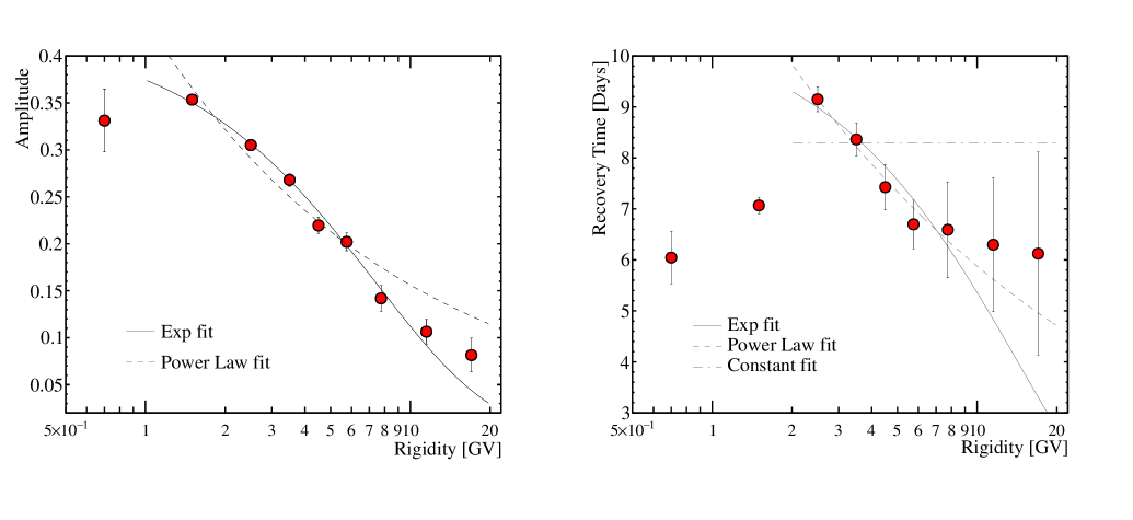
Figure 8: Left panel: the rigidity dependence of the Forbush decrease commencing the $2006$ December $14$ as measured by the PAMELA instrument. Each value results from an exponential fit (Equation 1) performed on the daily average time profile of the proton intensity. A total of nine rigidity intervals between $0.4$ and $20$ GV were studied. The solid and dashed black line represent an exponential (Equation 2) and a power law fit (Equation 3) respectively performed on the amplitude as a function of the rigidity. The parameters and the associated errors of the parameters obtained from the fit are displayed in Table 4.3. Right panel: as the left panel for the recovery time $\tau$. The dotted-dashed line represents a fit with a constant value (Equation 4).

The rigidity dependence of the amplitude and the recovery time were fitted by means of an exponential and a power law:

$$a\ e^{-\alpha R}$$ (2)

$$b\ R^{-\beta}$$ (3)

where $R$ is the rigidity and $a$, $\alpha$, $b$ and $\beta$ are free parameters to be determined. In addition the rigidity dependence of the recovery time was also fitted with a constant:

$$\eta$$ (4)

The solid black lines on Figure 8 (left and right panels) represent the exponential fits while the dotted lines refer to the power law fits. The dashed-dotted line in Figure 8 (right panel) represent the fit with a constant. The first point of the amplitude distribution and the first two points of the recovery time distribution were not used in the fits. The results of the fits are displayed in Table 4.3. From the $\chi^{2}$/NDF (number of degree of freedom) it can be noticed that the rigidity dependence of the Forbush decrease amplitude is better described with an exponential while the recovery time is well fitted with both a power law and an exponential fit. On the other hand the hypothesis of rigidity independence of the recovery time is heavely disfavoured from the $\chi^{2}$/NDF (see Table 4.3). The rigidity dependence of the recovery observed by PAMELA for the December $2006$ Forbush events was previously observed by Usoskin et al. (2008) combining observations from several neutron monitor stations (median rigidity between $10$ and $30$ GV) and the MUG muon telescope in Finland (mean rigidity of $55$ GV) and obtaining $\alpha=0.023\pm 0.007$.

It is generally thought that the main drivers of the recovery time are the decay of the interplanetary disturbance and to a lesser extent on the transport parameters of GCRs which would imply that the recovery time is not energy dependent (e.g. Loockwood et al. (1986); Wibberenz et al. (1998)). However, Mulder et al. (1986) argued that the Forbush decrease recovery time is affected by the interplanetary magnetic field polarity and thus the drift of GCRs in the heliosphere, which implicitly depends on energy. Our results for the December $2006$ Forbush event sustain this energy dependence of the recovery. Other recent results (e.g. Usoskin et al. (2008); Zhao and Zhang (2016)) found both events with and without energy dependence of the recovery concluding that this dependence is strongly related to the features of the solar disturbance causing the Forbush decrease.

4.3 Proton-electron-helium comparison

As already discussed in Section 1 the PAMELA instrument allows the Forbush decrease to be compared for different particle species. The proton intensity over time was compared to the electron and the helium intensities in order to highlight possible differences in the amplitude and the recovery time. The three left panels of Figure 4.3 show the comparison between the daily averaged proton intensity (full circles) and the two days average electron fluxes (full squares). In order to increase the limited electron statistics with respect to the analysis described in Section 4.2, the lower limit of the first rigidity interval was increased from $0.4$ GV to $0.6$ GV. Taking into account the discussion in Section 3 this was equivalent to increasing the total live time spent by the satellite at geomagnetic latitude suitable for detecting galactic particles. An overall increase of the live time of about $40\%$ was achieved. Moreover, the third rigidity interval was extended up to $5$ GV in order to increase the statistics.

The three right panels of Figure 4.3 show the proton intensity (circle points) compared with the helium intensity (square points). Because of the energy losses inside the apparatus, the PAMELA instrumental limit for helium detection is about $0.8$ GV. For this reason the first rigidity interval was chosen to be $1$-$2$ GV while the last one was $5$ - $10$ GV. In order to emphasize possible differences in the amplitude or the recovery time an exponential fit (Equation 1) was performed on the proton, electron and helium intensity profiles over time. The solid lines and the dotted lines in the left panels represent the proton and electron fits respectively, while in the right panels they represent the proton and helium fits respectively. The amplitude and the recovery time resulting from the fits as a function of rigidity are shown on left and right panel of Figure 10 respectively.

As can be seen in Figure 10 the helium and the proton amplitude and recovery time are in agreement within the errors for each rigidity interval. On the contrary electrons show a faster recovery time with respect to the protons for the first two rigidity intervals while having the same amplitude. The recovery time shows a better agreement between protons and electrons in the last rigidity interval ($2$-$5$ GV). This differences could be interpreted as an effect of the GCR propagation inside the heliosphere, in particular the charge sign dependence introduced by drift motions (Ferreira et al., 2004). In particular, since the near-Earth ICME extent was estimated to occupy a significant solid angle in the heliosphere, i.e. $74^{\text{\textopenbullet}}$ in latitude and $117^{\text{\textopenbullet}}$ in longitude (Liu et al., 2008) with respect to the heliospheric equator, possibly global drift motions may play a role in the recovery phase. In fact, during $A<0$ epochs such as in the declining phase of cycle 23, when the heliospheric magnetic field is directed toward the Sun in the northern hemisphere, negatively charged particles undergo drift motion mainly from the polar to the equatorial regions while positively charged particles drift mainly in the opposite directions.

Table 1: Fitted parameters for the rigidity dependence of $A$ and $\tau$ performed with Equations 2 and 3.

	Amplitude	Recovery Time
$\chi^{2}_{\text{exp}}$/NDF	$9.2/6$	$5.6/5$
$a$	$0.43\pm 0.01$	$10.7\pm 0.5$
$\alpha$	$0.134\pm 0.007$	$0.07\pm 0.02$
$\chi^{2}_{\text{powerlaw}}$/NDF	$41/6$	$1.5/5$
$b$	$0.43\pm 0.01$	$12.2\pm 0.9$
$\beta$	$0.45\pm 0.02$	$0.31\pm 0.06$
$\chi^{2}_{\text{constant}}$/NDF		$34/6$
$\eta$		$8.2\pm 0.2$

Moreover, as discussed above, at least two shocks and ICME combined during the period of the December $2006$ Forbush decrease , which would presumably occupy a larger extent than the single shock/ICME. Thus, considering the ICMEs topology just discussed, it can be argued that the equatorward electron drift direction would be expected to help fill in the Forbush decrease resulting in a faster recovery time with respect to the protons which drift mainly in the opposite direction and would experience a longer suppression. This result is in agreement with le Roux et al. (1991) who predicted that the recovery time is longer for positively charged particles when the polarity of the solar magnetic field is negative solving a 2D transport equation, including adiabatic cooling and particle drift. The charge sign dependence introduced by drift motions in the global solar modulation of GCRs, i.e. the ratio of GCRs intensities during opposite polarity cycle, is expected to have a maximum effects at around between $300$-$500$ MV becoming less than few $\%$ at $5$ GV (see e.g.. Adriani et al. (2016b); Di Felice et al. (2017); Nndanganeni et al. (2016)). This may explain why the differences in the recovery time between electrons and protons are greater at the lowest rigidities and tend to reduce as the rigidity increases.

Figure 9: Left panels: proton (full circles) and electron (full squares) time profile intensities for three different rigidity ranges during the December $2006$ Forbush decrease. The proton intensity is averaged over one day while the electron is averaged over two days. Right panels: as for the left panel with proton (full circles) and helium (full squares). The solid horizontal lines represent the reference intensity on which data were normalized (November $2006$). The solid and the dotted lines represent exponential fits performed with Equation 1 respectively to proton and electron in the left panels and to proton and helium in the right panels. In each panels the amplitude $A$ and the recovery time $\tau$ obtained with the exponential fit are reported. In both panels the lines connecting each point are displayed only to guide the eye.

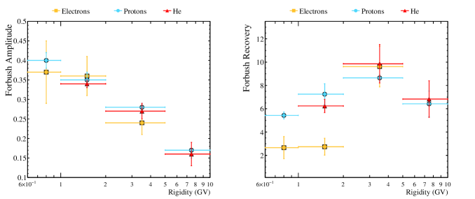
Figure 10: Left panel: the rigidity dependence of the December 2006 Forbush decrease amplitude for protons (circles), electrons (squares) and helium nuclei (triangles). Right panel: same as left panel for the recovery time.

5 Conclusion

For the first time a Forbush decrease ($2006$ December $14$) was extensively studied using observations of GCR in space with the PAMELA instrument. The proton observations have sufficient statistics to make it possible to study the temporal evolution of the event with three hours time resolution for different rigidity intervals between $0.4$ - $20$ GV. The rigidity dependence of the amplitude and the recovery time were investigated over nine different intervals. The amplitude of the Forbush decrease was found to decrease as the rigidity increased. An exponential fit describes well the rigidity dependence for the amplitude. The recovery time shows an increasing trend below one GV which could be either a limitation of the fitting procedure due to the contamination of the solar energetic particles or a real physical effect. Above 1 GV a general decreasing trend is found. Both the exponential and power law well fit this distribution.

For the first time the PAMELA observation allowed to study the behavior of different particle species during a Forbush decrease. In particular protons, helium nuclei and electrons were compared. The proton and the helium nuclei amplitude as well as the recovery time were found in good agreement while electrons showed on average a faster recovery time which tended to approach the proton recovery time as the rigidity increased. This behavior could be interpreted as a charge-sign dependence due to the different global drift pattern between protons and electrons.

The results discussed in this paper will be available at the Cosmic Ray Data Base of the ASI Space Science Data Center (http://tools.asdc.asi.it/CosmicRays/chargedCosmicRays.jsp).

We acknowledge partial financial support from The Italian Space Agency (ASI) under the program “Programma PAMELA - attivitá scientifica di analisi dati in fase E”. We also acknowledge support from Deutsches Zentrum fur Luft- und Raumfahrt (DLR), The Swedish National Space Board, The Swedish Research Council, The Russian Space Agency (Roscosmos) and Russian Ministry of Education and and NASA Supporting Research Grant $13-SRHSPH1320075$. M. S. Potgieter acknowledge the partial financial support from the South African Research Foundation (NRF) under the SA-Italy Bilateral Programme. I. G. Richardson acknowledges support from the ACE mission.

References

- Adriani et al. (2003) Adriani, O., et al. 2003, Nucl. Instrum. Methods A, 511, 72
- Adriani et al. (2011a) Adriani, O., et al. 2011a, Astrophys. Journal, 742, 102
- Adriani et al. (2011b) Adriani, O. et al. 2011b, Science, 332, 69
- Adriani et al. (2014) Adriani, O., et al. 2014, Phys. Rep., 544, 323
- Adriani et al. (2015) Adriani, O. et al. 2015, Astrophys. Journal, 810, 142
- Adriani et al. (2016a) Adriani, O. et al. 2016a, Space Weather, 14, 210
- Adriani et al. (2016b) Adriani, O. et al. 2016b, Phys. Rev. Lett., 116, 241105
- Adriani et al. (2017) Adriani, O. et al. 2017, RIVISTA DEL NUOVO CIMENTO, 40, 473
- Agostinelli et al. (2003) Agostinelli, S. , et al. 2003, Nucl. Instrum. Meth. A, 506, 250
- Arunbabu et al. (2013) Arunbabu, K. P. et al. 2013, A&A. , 555, A139
- Barnden (1976) Barnden, L. R. 1973, Proceedings of the 13th International Conference on Cosmic Rays, 2 , 1277
- Boezio et al. (2002) Boezio, M. et al. 2002, Nucl. Instrum. Methods A, 487 , 407
- Cane et al. (1993) Cane, H. V., Richardson, I. G. and von Rosenvinge, T. T. 1993, JGR, 98, 13295
- Cane et al. (1995) Cane, H. V., Richardson, I. G., Wibberenz, G. 1995, Proc. 24th International Cosmic Ray Conf. , 4, 377
- Cane (2000) Cane, H. V. 2000, Space Science Reviews, 93 , 55
- Di Felice et al. (2017) Di Felice, V. , Munini R., Vos E. E. and Potgieter M. S., 2017, Astrophys. J., 834, 89
- Ferland et al. (2013) Ferland, G. J., Porter, R. L., van Hoof, P. A. M., et al. 2013, Rev. Mexicana Astron. Astrofis., 49, 137
- Forbush (1937) Forbush, S. E. 1937, Phys. Rev, 51, 1108
- Ferreira et al. (2004) Ferreira, S. E. S., Potgieter, M. S. 2004 , ApJ., 603 , 744
- Hathaway (2015) Hathaway, D. A. 2015, Living Reviews in Solar Physics, 12, 4
- Hess and Demmelmair (1937) Hess, V. F., Demmelmair, A. 1937, Nature, 140, 316
- Jämsén et al. (2007) Jämsén, T., Usoskin, I.G., Räihä, T., Sarkamo J, Kovaltsov, G.A. 2007, Advances in Space Research, 40, 342
- Jian et al. (2006) Jian, L., Russell, C. T., Luhmann, G., Skoug R. M. 2006 , Solar Physics, 239, 393
- Klein and Burlaga (1982) Klein, L.W., Burlaga, L.F. 1982 , J. Geophys. Res., 87, 613
- Krittinatham et al. (2009) Krittinatham, W., Ruffolo, D. 2009 , Astrophys. J., 704, 831
- Kubo et al. (2010) Kubo, Y., Shimazu, H 2010 , Astrophys. J., 720, 853
- Mulder et al. (1986) Mulder, M. S., Moraal, H. 1986 , ApJL, 330, L75
- le Roux et al. (1991) Le Roux, J. A., Potgieter, M. S. 1991 , A&A , 243 , 531
- Liu et al. (2008) Liu, Y. et al. 2008 , The Astrophysical Journal , 689 , 563
- Loockwood et al. (1986) Loockwood, J. A., Webber, W. R., Jokipii, J. R. 1986 , JGR , 91
- Luo et al. (2017) Luo, X., Potgieter, M. S., Feng, X. 2017 , ApJ , 893, 53
- Orsi et al. (2005) Orsi, S. et al. 2005, Proc. 29th ICRC (Pune), 3, 369
- Osteria et al. (2004) Osteria, G. et al. 2004, Nucl. Instrum. Methods A , 535, 152
- Parker (1963) Parker, E. N. 1963, Interplanetary Dynamical Processes, Interscience Publishers, New York
- Picozza et al. (2007) Picozza, P. et al. 2007 Astropart. Phys. 27 , 296
- Potgieter (2013) Potgieter, M. S. 2013, Living Reviews in Solar Physics, 10 , 3
- Potgieter et al. (2014) Potgieter, M. S., Strauss, R. D. 2014, Sol Phys, 289
- Reames (1996) Reames, D. V. 1999, Space Sci. Rev., 90, 413
- Nndanganeni et al. (2016) Nndanganeni, R. R., Potgieter M. S. 2016, Advances in Space Research, 58, 453
- Richardson (2004) Richardson, I. G. 2004, Space Science Reviews, 111 , 267
- Richardson and Cane (2010) Richardson, I. G., Cane, H. V. 2010, Solar Phys., 264 , 189
- Richardson et al. (2011) Richardson, I. G., Cane H. V. 2011, Solar Physics, 270 , 609
- von Rosenvinge et al. (2009) von Rosenvinge, T. T. et al. 2009, Solar Phys, 256, 443
- Russell et al. (2010) Russell, C. T., Luhmann, J. G., Jian, L. K. 2010, Reviews of Geophysics, 48
- Shea et al. (1987) Shea, M. A., Smart, D. F., Gentile, L. C. 1987, Physics of the Earth and Planetary Interiors, 48, 200
- Simpson (1998) Simpson, J. A. 1998, Space Sci. Rev., 83, 169
- Stozhkov et al. (2005) Stozhkov, Y. et al. 2005, Int. J. Mod. Phys. A, 20, 6745
- Thomas et al. (2005) Thomas, S. R. et al. 2015, The Astrophysical Journal, 801, 5
- Usoskin et al. (2008) Usoskin I. G. et al. 2008, Proc. 30th International Cosmic Ray Conf, 1, 327
- Vieira et al. (2012) Vieira, L. R. et al. 2012, Advances in Space Research, 49, 1615
- Wibberenz et al. (1997) Wibberenz, G., Cane, H. V. and Richardson, I. G. 1997, Proc. 25th International Cosmic Ray Conf. , 4, 397
- Wibberenz et al. (1998) Wibberenz, G., Le Roux, J. A., Potgieter, M. S., Bieber, J. W. 1998, Space Science Review, 83, 309
- Zhao and Zhang (2016) Zhao, L.-L, Zhang, H. 2016, The Astrophysical Journal, 827, 13