Holographic meson decays via worldsheet instantons

Abstract

We study meson decays using instanton methods in two string models. The first model is the old string model in flat space which combines strings and massive particles and the second is the holographic, Sakai-Sugimoto model. Using the the old string model, we reproduce the QCD formula for the probability of splitting of the QCD flux tube derived by Casher-Neuberger-Nussinov (CNN). In the holographic model we construct a string worldsheet instanton which interpolates between a single and double string configuration, which determines the decay from one to two dual mesonic particles. The resulting probability for meson decay incorporates both the effects of finite meson size as well as back-reaction of the produced quarks on the QCD flux tube. In the limit of very large strings the probability for a split reduces to the CNN formula. A byproduct of our analysis is the analysis of the moduli space of a generic double concentric Wilson loop with circles which are separated in the holographic direction of the confining background.

1 Introduction

The holographic approach offers a framework to address some of the most challenging questions in strongly coupled gauge theories in a (semi) analytic way. While most of the work in the holographic approach has taken place in the context of supersymmetric theories, the expectation is that similar methods can be applied to study of strongly coupled phenomena in QCD. At the moment the geometry which is dual to QCD is not yet known. However, there are proposals for dual geometries which capture various qualitative features of QCD. One of the most successful dual models is the Sakai-Sugimoto model Sakai and Sugimoto (2006) which is special in the sense that it incorporates chiral symmetry breaking in the dual description.

In this paper we have used the Sakai-Sugimoto model to compute probabilities for decays of mesonic particles, via breaking of flux tubes. As this process is a strongly coupled phenomenon, its computation in QCD is not easily performed. Yet, knowing the probability for a flux tube to break is crucial for understanding both the decay widths of mesons and the hadronisation phase in high-energy scattering processes. A long time ago, a very successful phenomenological model, the Lund fragmentation model Sjöstrand (1982); Andersson et al. (1983) was developed in order to model hadronisation in event generators for high-energy collisions. In this model, mesons are modelled by two (massive) particles which are connected by a relativistic string, which models the QCD flux tube. In a high-energy collision, the pair-produced quark and antiquark move away from each other, with the colour string stretching between them. As the string becomes longer, it eventually snaps, producing a new quark-antiquark pair and so on, leading to a shower of mesonic particles.

The probability for a string to break at particular point was “derived” by Casher, Neuberger and Nussinov (CNN) in the early days of QCD Casher et al. (1979). The formula was written down by making an analogy with electromagnetism: the electric field in the Schwinger formula was replaced with an (abelianised) chromoelectric field and quarks were treated as free charged particles which are minimally coupled to this field. While this model agrees qualitatively with experimental data, it contains several free parameters which need to be fixed by comparison with experiment. A holographic approach may potentially shed some light on the origin of these free parameters.

The probability for a QCD string to break by producing a quark-antiquark pair is also relevant when computing the lifetime of mesons. In the Sakai-Sugimoto model, large-spin mesons are modelled by macroscopic, rotating, U-shaped strings with endpoints which are stabilised from collapse by a centrifugal force and are constrained to “move” on probe D8-branes, see figure 3. The probability for such a string to split can be computed in two ways. In our previous work Peeters et al. (2006); Sonnenschein and Weissman (2018) we used a string bit model, in which we computed the probability for a string to fluctuate in the holographic direction and hit the probe brane. As it hits the probe, the string can split with some probability. The resulting decay width $\Gamma$ was found to exhibit exponential suppression in the masses of the pair-produced quarks and linear dependence on the effective length of the QCD string flux tube. Wave-function based approaches as in Peeters et al. (2006) are, however, numerically hard to handle in the continuum limit, where the number of string beads is large. In addition, the computations of string fluctuations in Peeters et al. (2006) were for computational reasons restricted to the near-wall region where the background metric is linearised around flat space.

In order to improve on these points, we initiate in the present paper an alternative, instanton approach to the study of holographic breaking of the QCD flux tube. That is, we will construct a string worldsheet instanton which interpolates between the unsplit and split U-shaped mesonic strings. As in Peeters et al. (2006), we consider a simplified system, which is represented by a hanging U-shaped string, which does not rotate but is prevented from collapse by a Dirichlet boundary condition. Such a system is similar to the strings used in the original Lund model, which was initially also applied to non-rotating systems. The instanton configuration has the geometry of a cylindrical surface, with circular boundaries which are concentric in the field theory directions, and separated from each other in the holographic direction of the dual geometry. A generic instanton configuration would take into account the backreaction of the produced quarks on the flux tube, through the bending of the flux tube in the holographic direction. Our instanton describes the decay of a finite-size flux tube and finite-volume mesonic particle in which the endpoint quarks accelerate from each other.

The CNN formula does not take into account backreaction of the pair-produced quarks and it also deals with an infinitely long flux tube. In the large volume limit, the QCD flux tube is much longer than the radius at which the quarks are pair-produced and one expects that the dynamics of the external quarks is decoupled from the string breaking process. The probability is then fully determined by the property of the tube and does not depend on the quarks in the original meson. In order to compare our findings with the results of CNN, we have therefore also investigated the large-volume limit of our result, in which we indeed reproduce the simple exponential suppression of the decay probability with the square of the quark mass, $\exp(-m_{q}^{2}/T)$, where $T$ is the tension of the string Casher et al. (1979).

Our paper is organised as follows. In section 2 we first review the key features of the worldline derivation of the Schwinger pair production formula Affleck et al. (1982) and its generalisation to QCD Casher et al. (1979). In section 3 we consider, as a warm-up exercise, the old string model with massive endpoints in flat space, and construct the instanton configuration which reproduces results of Casher et al. (1979). In section 4 we construct a similar instanton configuration in the Sakai-Sugimoto model and compute from it the probability for meson decay. Our main findings and open questions are discussed in the last section.

2 QCD string breaking à la Schwinger in flat spacetime

It has been known for a long time that the presence of an external electric field leads to the production of electrically charged particle-antiparticle pairs Schwinger (1951). While the original computation of Schwinger was done by perturbatively summing a class of one-loop diagrams in quantum field theory, the same result was later rederived in the worldline approach, by construction of a worldline instanton Affleck et al. (1982). The same worldline instanton approach was also used to describe the production of monopole/anti-monopole pairs in an external magnetic field Affleck and Manton (1982).

In this section we will briefly review the basic derivation of the Schwinger result for a production of particle-antiparticle pairs in an external electric field, using the worldline instanton approach Affleck et al. (1982). We then review an application of this formula to the pair production of quark-antiquark pairs inside the QCD flux tube following the seminal work of Casher et al. Casher et al. (1979).

Assume that a non-vanishing electric field $E$ is turned on in the $X^{1}$ direction. In order to construct the worldline instanton describing the production of a particle-antiparticle pair of masses $m$ and charge $q$, one needs to consider the Wick rotated system obtained by $\tau\rightarrow-i\tau$, $A_{0}\rightarrow-iA_{0}$ and solving the classical equations of motion of a particle in the Euclidean background with $F_{01}=-iE$. The action of the particle is given by

$$S_{E}=\int\!{\rm d}\tau\,\bigg{(}m\sqrt{\dot{X}^{\nu}\dot{X}_{\nu}}-iqA_{\nu}\dot{X}^{\nu}\bigg{)}\,.$$ (1)

It is not hard to see that the solution for the particle worldline is given by

$$X^{0}(\tau)=R\cos(2\pi n\tau)\,,\quad X^{1}(\tau)=R\sin(2\pi n\tau)\,,\quad X^{2}=0\,,\quad X^{3}=0\,,$$ (2)

where $X^{0}$ is the Wick rotated target space time direction and $R$ is fixed in terms of $E$ by the equation of motion, see below. We see that the worldline instanton looks like a loop of radius $R$. The parameter $n$ labels different instantons, and describes how many times the particle “winds” around the loop. As usual, the particle propagating “backwards” in the (Euclidean) time $X^{0}$ is interpreted as an antiparticle. Hence, the left-hand side of the loop can be interpreted as the worldline of the antiparticle, while the right-hand side as the worldline of the particle, see figure 1.

Substituting the solution (2) into the particle action (1) and integrating over the worldline gives

$$S_{\text{class}}=2\pi nRm-\pi nqER^{2}\,.$$ (3)

The extrema of the action will give classical solutions, and one finds that the radius of the loop is fixed to be $R=m/(qE)$ for which the action reduces to $S_{\text{class}}=\pi\frac{m^{2}}{qE}n$.

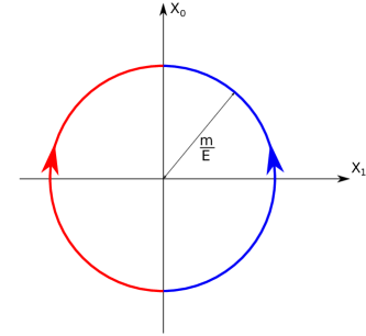
Figure 1: Worldline instanton for particle-antiparticle pair production in an external electric field $E$.

So the full loop (2) describes a particle-antiparticle pair which is produced at the Euclidean time $X^{0}=-R$, in which the particles move away from each other. Once the particle and antiparticle go on-shell, i.e. once they reach a distance $2m/(qE)$, one can analytically continue the solution (2) back to Lorentzian time. The Lorentzian solution describes a pair of particles accelerating away from each other with proper acceleration $a=m/(qE)$.

Exponentiation of this Euclidean action $S_{\text{class}}$ with winding $n=1$ gives the most dominant contribution for the probability of particle production in the saddle point approximation. Looking at the fluctuations around this classical path (2), and summing over their contributions in the path integral Affleck et al. (1982), produces a pre-factor to the exponent $e^{-S_{\text{class}}}$, and one obtains the celebrated Schwinger formula for the probability of production of particles. The probability for the pair production of particles of spin half and charge $q$, per unit volume and per unit time, is given by Schwinger (1951)

$$P_{\text{pp}}=\frac{E^{2}}{8\pi^{3}}\sum_{n=1}^{\infty}\frac{1}{n^{2}}e^{-\frac{\pi m^{2}}{q|E|}n}\,.$$ (4)

A long time ago, Casher et al. Casher et al. (1979) argued that the Schwinger pair production formula (4) can be directly applied to QCD in order to derive a formula for the decay of mesons. In their set up, Casher et al. assumed that at the hadronic energy scale of $1$ GeV the quarks inside mesons can be treated as Dirac particles with constituent masses $m$ and charge $q$. They also assumed that at timescales which are short compared to the hadronic timescale, mesons can be modelled as chromo-electric flux tubes (“thick strings”) of universal thickness such that the chromo-electric field can be treated as a classical, constant, longitudinal abelian field. Hence the process of meson decay can be seen as Schwinger pair production of quark-antiquark pair, by the (abelianised) QCD field.

The flux tube is parametrised by the radius $r_{t}$, the “abelianised” QCD field strength $\mathcal{E}_{t}$ and the gauge coupling $g$ which is related to the charge of the quarks $q$ as $q=g/2$. It has been argued that the reason for the factor $1/2$ between $g$ and $q$ is the fact that quarks couple to the gauge field through the $SU(3)$ generators $\lambda^{a}/2$. The energy per unit length stored in the tube is the effective tube (string) tension and is given by

$$\gamma_{\text{QCD}}=\frac{1}{2\pi\alpha^{\prime}}=\frac{1}{2}\mathcal{E}_{t}^{2}\pi r_{t}^{2}\,,$$ (5)

$\gamma_{\text{QCD}}\sim 0.177(\text{GeV})^{2}$ and the radius of the tube is $r_{t}\sim 2.5\text{GeV}^{-1}$. On the other hand, using the (abelian) Gauss law and the fact that flux lines are non-vanishing only between the quarks (like for a capacitor), one has $\mathcal{E}_{t}\pi r_{t}^{2}=q=g/2$ which implies that the effective tension of the flux tube is

$$\gamma_{\text{QCD}}=\frac{1}{2}\mathcal{E}_{t}q\,.$$ (6)

Hence the Schwinger formula (4) can be rewritten in terms of the natural QCD variables as

$$P_{\text{QCD}}=\frac{\gamma_{\text{QCD}}}{\pi^{3}}\sum_{n=1}^{\infty}\frac{1}{n^{2}}e^{-\frac{\pi m_{q}^{2}}{2\gamma_{\text{QCD}}}n}\,.$$ (7)

We should comment at this stage that the factor of $1/2$ in the exponent is a consequence of the fact that the QCD field in the flux tube has been treated as an abelian field. In the more recent paper Nayak (2005), a proper generalisation of the Schwinger formula to a non-abelian field has been derived and the production rate has been shown to depend on two independent Casimir gauge invariants $E^{a}E^{a}$ and $d_{abc}E^{a}E^{b}E^{c}$. In what follows we will see that the holographic model reproduces the exponential dependence of the production rate in (7), up to this numerical factor.

From the formula (7), the probability for a meson to decay after time $t$, measured in the meson rest frame, is $1-e^{-V_{4}(t)P_{QCD}}$ where $V_{4}(t)$ is the four-volume spanned by the system until time $t$. For a meson which is modelled by a rotating flux tube of lenght $L$, this volume is $V_{4}(t)=\pi r_{t}^{2}Lt$. Therefore, the decay width (probability per unit time) is $\Gamma=\pi r_{t}^{2}LP_{\text{QCD}}$. Because the meson mass is $M=\pi\gamma_{\text{QCD}}L$, one finds that the ratio of decay width $\Gamma$ and the meson mass $M$ is independent of the effective length of the string,

$$\left(\frac{\Gamma}{M}\right)_{\text{rot}}=\frac{2r_{t}^{2}}{\gamma_{\text{QCD}}}P_{\text{QCD}}\,.$$ (8)

Similarly, modelling mesons as one-dimensional oscillators implies $(\Gamma/M)_{\text{osc}}=\pi/4(\Gamma/M)_{\text{rot}}$, so that the ratio is independent of the effective size of the sysem. At the moment, the experimental data on meson decays do not agree with this prediction for lighter mesons (see the discussion in Peeters et al. (2006); Sonnenschein and Weissman (2018)), while for high-spin mesons, where one would expect this model to work bettter, the data are not accurate enough to confirm or reject such a prediction.

3 Worldsheet instanton in flat space and string splitting

While our main goal is to study meson decays in the holographic setup, we will as a warm up exercise first consider the process of meson decay in flat space without using the analogy with the Schwinger formula. This will provide an alternative, new derivation of the formula (7) which, to the best of our knowledge, has so far not been presented elsewhere.

In order to model mesons, including their flux tube as well as endpoint quarks, we will use an action for the relativistic string suplemented with two massive particles which are attached to the string endpoints. This is the “old” string model, as discussed and reviewed in Barbashov and Nesterenko (1990). We want to find the Euclidean worldsheet configuration which interpolates between the unsplit and split string with massive end points. After performing a Wick rotation in the target and worldsheet space-time, the string action becomes

$$S =\gamma\int_{\tau_{1}}^{\tau_{2}}\!{\rm d}\tau\,\int_{0}^{\pi}d\sigma\sqrt{-(\dot{X}\cdot X^{\prime})^{2}+\dot{X}^{2}X^{\prime 2}}$$ (9)

$$\qquad\qquad+m\int_{\tau_{1}}^{\tau_{2}}\!{\rm d}\tau\bigg{(}\sqrt{\dot{X}^{2}(\tau,\sigma=0)}+\sqrt{\dot{X}^{2}(\tau,\sigma=\pi)}\bigg{)}$$

$$\equiv S_{\text{bulk}}+S_{\partial,\sigma=0}+S_{\partial,\sigma=\pi}\,.$$

Here $X\cdot X\equiv X^{\mu}X^{\nu}g_{\mu\nu}(X)$ and $g_{\mu\nu}(X)$ denotes the Euclidean metric in the target space, which for us at this stage is just a flat metric, $g_{\mu\nu}=\delta_{\mu\nu}$. The tension of the string is denoted with $\gamma=1/(2\pi\alpha^{\prime})$ and $m$ is the mass of the particles attached to the string endpoints.

We are interested in finding a Euclidean, two-dimensional string configuration which interpolates between a single and a double string. The initial string had only two quarks at its endpoints. In the fully dynamical string model, the position of these outer quarks is fixed by the total angular momentum of the meson, which prevents strings from collapsing, see for example Barbashov and Nesterenko (1990). To simplify the discussion, we will in this paper take quarks in the original meson to satisfy Diriclet boundary conditions and confine them to move on a line in the Euclidean target space.

At some point in the Euclidean “time”, a pair of massive quarks is pair-produced in the interior of the string. These particles represent new “internal” endpoints of the string, which can move freely, i.e. satisfy Neumann boundary conditions, see figure 2. In order to account for the pair-produced quarks, one needs to modify the action (9) by adding to it the worldline action of the pair-produced quarks. Adding this extra term in the action is in spirit the same as what one does in order to describe the pair-production of the charged particle-antiparticle pair in the external electric field using the instanton approach in the world-line formalism, see e.g. Semenoff and Zarembo (2011). The main difference is that the role of the electric field is now played by the tension of the split string, which pulls apart the pair-produced particles. For simplicity, we will also assume that the particles have no transverse momentum, so that the whole process of string splitting is planar, i.e. that both in- and outgoing strings are in the same two-dimensional plane.

As the variation of the action (9) leads to bulk and boundary equations of motion we have to make sure that both are satisfied. In the two-dimensional target space, the bulk equations of motion are always satisfied, thanks to reparametrisation invariance of the action. So we just need to make sure that the boundary equations of motion for the Neumann boundary conditions hold. Note that the boundary equations of motion receive nontrivial contribution from the surface terms of the bulk part of the action,

$$\frac{\partial\,\,\,}{\partial\tau}\left(\frac{\partial\mathcal{L}_{\partial,\sigma_{B}}}{\partial\dot{X}^{0}}\right)-\frac{\partial\mathcal{L}_{\text{bulk}}}{\partial{X^{\prime}}^{0}}\Bigg{|}_{\sigma_{B}}=0\,,$$ (10)

where $\sigma_{B}$ is the position of the boundary (or boundaries) of the string for which Neumann conditions are imposed.

Before the quarks were pair-produced, the string was straight and stretching between $(0,2L)$ in the target space. To describe this string configuration we choose the parametrisation

$$X^{0}=\tau\,,\quad\quad X^{1}=2L\frac{\sigma}{\pi}\,,\quad\quad\sigma\in[0,\pi\rangle\,.$$ (11)

The instanton configuration for a splittting string is plotted in figure 2, and is given by

$$X_{L}^{0}(\tau,\sigma) =X_{R}^{0}(\tau,\sigma)=\tau\,,$$ (12)

$$X_{L}^{1}(\tau,\sigma) =x_{L}(\tau,\sigma)=-\frac{\sigma}{\pi}\left(\sqrt{-\tau^{2}+\kappa^{2}}-a\right)\,, \sigma\in[0,\pi\rangle\,,$$

$$X_{R}^{1}(\tau,\sigma) =x_{R}(\tau,\sigma)=\left(1-\frac{\sigma}{\pi}\right)\left(\sqrt{-\tau^{2}+\kappa^{2}}+a\right)+2a\frac{\sigma}{\pi}\,, \sigma\in[0,\pi\rangle\,,$$

where $\kappa$ and $a$ are arbitrary constants, and $X_{L}$ and $X_{R}$ describe left and right half of the instanton (the red and blue areas in figure 2). Note that while we have written the solution piece-wise, the two “sides” of the instanton, $X_{L}$ and $X_{R}$ are glued in a smooth way. The solution above is a Euclidean version of a solution found in Bardeen et al. (1976).

It is easy to see that the ansatz (12) satisfies the Neumann boundary equations of motions (10),

$$-m\frac{\partial\,\,\,}{\partial\tau}\left(\frac{\dot{X}_{L}^{\mu}(\tau,\sigma=\pi)}{\sqrt{1+\dot{x}_{L}^{2}(\tau,\sigma=\pi)}}\right)+\gamma\left(-\dot{x}_{L}\dot{X}_{L}^{\mu}+\left(\frac{1+\dot{x}_{L}^{2}}{x_{L}^{\prime}}\right)X_{L}^{\prime\mu}\right)\bigg{|}_{\sigma=\pi}=0\,,$$ (13)

(where $\mu=0,1$) provided that $\kappa=m/\gamma$. A similar expression holds for the right-hand piece $X_{R}^{\mu}$. Note also that the solution (12), where the outer quarks are moving on straight lines, can be generalised to a solution for which the endpoints do not follow straight lines but move on arbitrary curves $f_{L}(\tau)$ and $f_{R}(\tau)$, see figure 2b.

$$X_{L}^{0}(\tau,\sigma) =X_{R}^{0}(\tau,\sigma)=\tau\,,$$ (14)

$$X_{L}^{1}(\tau,\sigma) =x_{L}(\tau,\sigma)=-\frac{\sigma}{\pi}\left(\sqrt{-\tau^{2}+\kappa^{2}}-a\right)+f_{L}(\tau)\left(1-\frac{\sigma}{\pi}\right)\,,\quad \sigma \in(0,\pi)\,,$$

$$X_{R}^{1}(\tau,\sigma) =x_{R}(\tau,\sigma)=\left(1-\frac{\sigma}{\pi}\right)\left(\sqrt{-\tau^{2}+\kappa^{2}}+a\right)+f_{R}(\tau)\frac{\sigma}{\pi}\,,\quad \sigma \in(0,\pi)\,,$$

with $\kappa=m/\gamma$ as above. We therefore see that in whichever way the outer quarks move, the dynamics of the inner free (Neumann) quarks is unaffected. The “motion” of the inner quarks is always circular, with a radius of curvature which is determined by the ratio of the particle mass and the string tension which pulls the produced quarks.

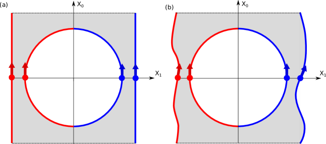
Figure 2: Flat space instantons, describing the breaking of the string flux tube. The instanton on the left describes breaking of the flux tube where the external quarks are at a fixed distance, while the instanton on the right depicts external quarks which “move” on arbitrary paths.

In order to evaluate the probability for a single event of particle pair production, we need to evaluate the action of the instanton. The string configuration (12) describes the process of pair production inside the string, as well as the propagation of the outer, background quarks. Hence in order to isolate the part which describes particle production, we need to subtract the contribution corresponding to the background. In other words, the quantity of interest which gives us the probability for the particle production is

$$S_{\text{pp}}=S_{\text{full}}-S_{\text{background}}=m(\mathrm{Circumference}\,\,\mathrm{of}\,\,\mathrm{circle})-\gamma(\mathrm{Area}\,\,\mathrm{of}\,\,\mathrm{circle})\\[4.30554pt] =m(2\pi\kappa)-\gamma(\pi\kappa^{2})=\frac{\pi m^{2}}{\gamma}\,.$$ (15)

Here $S_{\text{background}}$ is the action of the background configuration with no particle production (11), $S_{\text{full}}$ is the action of the instanton configuration (13) and $\gamma$ is the string tension. It is easy to see that the same result is obtained with the more general solution (14), where the outer quarks move on arbitrary, non-straight paths. In other words, the dynamics of the external quarks is fully decoupled from the production process inside the flux tube.

We thus find that the probability for a single pair production event to happen is given by

$$P_{\text{PP}}=e^{-S_{\text{pp}}}=e^{-\frac{\pi m_{q}^{2}}{\gamma}}\,,$$ (16)

We see that this is the as the contribution of a single instanton in the CNN formula (7), up to a numerical factor of a half. So we see that in the process of string splitting, the string tension has the same role as the electric field in the Schwinger process, that is, it pulls the produced particles away from each other. However, note again that there is a difference with respect to the Schwinger process, as quarks couple to the string endpoints in a different way than described by minimal coupling to electromagnetism (as used in the CNN approach).

The position of the instanton can be at any arbitrary point on the string worlsheet, as long as the instanton is not too close to the boundary of the string worldsheet, so that size of the instanton circle “fits” into the string worldsheet. One can therefore compute the probability per unit time $\Gamma$ from the the probability per unit volume and unit time (16) as $\Gamma=P_{\text{pp}}L$ where $L$ is the string length. On the other hand, the mass of the initial mesonic “particle” is $M=\gamma L+2m$, where $m$ is the mass of the initial quark pairs. In the limit of long strings ($L\gg m/\gamma$) one can approximate $M\approx\gamma L$ and also ignore subtleties related to whether the instanton fits into the worldsheet or not. In this limit one recovers the results from the previous section as well as from the holographic computation of Peeters et al. (2006), namely that $\Gamma/M$ is a constant for all mesonic particles.

In summary, we have constructed a flat space instanton configuration which describes splitting of the open relativistic string with the massive endpoints, into two strings with massive endpoints. The probability for such a process to occur is the same as the probability for pair production of charged massive particles in an external electric field of a strength which is proportional to the tension of the string.

4 String splitting in the Sakai-Sugimoto holographic model

Our discussion of splitting strings was so far done in flat space using the old string model of mesons. In holographic models of QCD, like the Sakai-Sugimoto model, mesons are incorporated by adding one or more flavour D8 probe branes in the holographic background which is dual to the confining, pure glue theory at strong coupling Sakai and Sugimoto (2006). In this setup the mesons appear either as light fluctuations of the probe D8-brane in the supergravity (DBI) approximation or as semi-classical string configurations of relativistic strings whose worldsheets end on the probe brane. Light DBI excitations of the probe brane describe mesons up to spin one, while higher-spin mesons are described by semi-classical strings. In what follows we will focus on the phenomenologically more interesting case of higher-spin mesons and their decay by constructing string worldsheet instanton configurations in the holographic background.

4.1 Review of high-spin mesons in the Sakai-Sugimoto model

The background geometry in which probe D8-branes and large strings are embedded is given by

$${\rm d}s^{2}=\left(\frac{u}{R_{D_{4}}}\right)^{3/2}\left(-{\rm d}t^{2}+\delta_{ij}{\rm d}x^{i}{\rm d}x^{j}+f_{\Lambda}(u){\rm d}x_{4}^{2}\right)+\left(\frac{R_{D_{4}}}{u}\right)^{3/2}\bigg{(}\frac{{\rm d}u^{2}}{f_{\Lambda}(u)}+u^{2}{\rm d}\Omega_{4}\bigg{)}\,,\\[4.30554pt] f_{\Lambda}(u)=1-\frac{{u_{\Lambda}}^{3}}{u^{3}}\,,\quad\quad i=1,2,3\,,$$ (17)

where ${\rm d}\Omega_{4}$ is the metric on a round four sphere. There is also a non-constant dilaton and a RR four-form field strength,

$$e^{\phi}=g_{s}\left(\frac{u}{R_{D_{4}}}\right)^{3/4}\quad\quad F_{4}=\frac{2\pi N_{c}}{V_{4}}\epsilon_{4}\,.$$ (18)

Here $R_{D_{4}}^{3}=\pi g_{s}N_{c}l_{s}^{3}$, $g_{s}$ is the string coupling and $l_{s}^{2}=\alpha^{\prime}$ is the string length. Here $u$ is the “holographic” direction, which is bounded from below by $u\geq u_{\Lambda}$. The world volume, non-holographic, directions in which the gauge theory lives are $t,x_{1},x_{2},x_{3}$. One of the main properties of this background is the cigar-like submanifold spanned by the periodic coordinate $x_{4}$ and the holographic direction $u$. The tip of the cigar is positioned at $u=u_{\Lambda}$ where the $x_{4}$ circle (smoothly) shrinks to zero size. One usually refers to the region near $u_{\Lambda}$, as the “wall”.

In order to incorporate quark/flavour degrees of freedom to this pure glue theory, one needs to place probe flavour $D8$ brane(s) in this geometry. There are different ways in which one can embed flavour $D8$ branes in this background. For us, the relevant embedding of the probe flavour $D8$ brane is the one in which $D8$ brane fills out all directions except the cigar $(u,x_{4})$ submanifold. In the cigar submanifold, the flavour $D8$ brane has a U-shape, see figure 3, with the tip of the probe brane which is at some distance $m_{q}$ from the wall $u_{\Lambda}$, see Sakai and Sugimoto (2006). In principle this parameter $m_{q}$ is a free parameter for the embedding of the brane, and can be changed by changing the asymptotic separation between the endpoints of the probe, see figure 3.

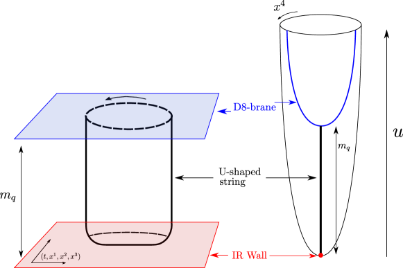
Figure 3: Sakai-Sugimoto background with the probe D8-brane and the U-shaped, mesonic string which hangs in the holographic direction towards the wall at $u=u_{\Lambda}$.

Large spin mesons correspond to rotating strings, whose endpoints are fixed on the flavour D8-brane. The strings are prevented from collapsing by a centrifugal force Kruczenski et al. (2005). As the spin of the string is increased, the distance between the string endpoints increases as well, i.e. the string becomes larger and its worldsheet becomes and more and more U-shaped. The two “vertical” parts of the string stretch almost vertically from the probe brane to the wall and the horizontal part of the string stretches almost parallel to the wall, see figure 3. It was shown in Kruczenski et al. (2005) that this string configuration is holographically equivalent to the system of two quarks which are connected by a flux tube, i.e. to the same model we have analysed in the previous section. By analysing the mass of this string configuration, it was shown that the vertical parts of the string correspond the (bare) quark masses of the meson, while the horizontal part of the string corresponds to the energy stored in the QCD flux tube.

In order to model a system with different quark masses for the two quarks, one needs to introduce more than one flavour D8-brane, each hanging at different distance from the wall. The positions of these probes in the holographic diretion specify different quark masses. A meson with different quark masses is then a string with endpoints ending on these two different flavour D8-branes.

We would now like to study the decay of such a string configuration. The hanging string is subject to quantum fluctuations and when a part of the string worldsheet touches one of the flavour branes it can split and attach new endpoints to that flavour brane. The probability for a string to touch the flavour brane due to quantum fluctuations was computed in Peeters et al. (2006) by constructing the string wave-function using a string bead model for a discretised string worldsheet.

Our approach here will be different. We will here construct a configuration of the Euclidean worldsheet, which interpolates between the single and double U-shaped strings, that is, a worldsheet instanton.

4.2 String worldsheet instanton

Our main goal is to holographically compute the probability per unit volume and time for a QCD flux tube to break. As in our previous analysis Peeters et al. (2006) and as in the flat space construction from the previous section, we simplify the problem by looking at a U-shaped string with endpoints which are “forced by hand” to follow a circular path of some radius. Imposing these boundary conditions is not unreasonable, as in the Lorentzian picture these correspond to quarks which accelerate away from each other with constant acceleration, as it happens in the hadronisation phase in high-energy scattering processes.

Generically the string breaking process will be sensitive to the precise boundary conditions one imposes for the external quarks. However, one would expect that there is a limit in which the exact dynamics of the external quarks decouples from the breaking process (a sort of large volume limit), so that the quark production process in this limit can be treated as a Schwinger process in a constant external field, like in Casher et al. (1979). As it is a priori not clear what this limit is or whether it exists in our setup, our approach will be to first construct the general solution and compute the decay probability for an arbitrary mesonic particle, and then see if there is a limit in which this probability reduces to the Schwinger probability.

A string can break only at the point where the interior of the world sheet touches the probe D8-brane. In real time such a situation happens because under quantum fluctuations, parts of the string worldsheet touch the probe brane. In the Euclidean setup, in order to construct the instanton configuration for a splitting string, one needs to start with the string worldsheet which is “pinned” to the D8 probe at some internal worldsheet point. So we impose Dirichlet boundary conditions in $u$ and $x_{4}$ directions both for the string endpoints and for the “pinning point”. Once the string has split at the pinning point, the newly generated string endpoints are free to “move” in the D8 worldvolume directions ($x_{0},x_{1},x_{2},x_{3}$ and $S^{4}$) freely, i.e. they satisfy Neumann boundary conditions.

In order to construct worldsheet instanton, we need to solve the string equations of motion in the Wick rotated background (17). It will be convenient to change to background coordinates as follows,

$$z=\frac{1}{u}\,,\quad\quad z_{D_{4}}=\frac{1}{R_{D_{4}}}\,,\quad\quad z_{\Lambda}=\frac{1}{u_{\Lambda}}\,,$$ (20)

which turns the metric into

$${\rm d}s^{2}=\left(\frac{z_{D_{4}}}{z}\right)^{3/2}\bigg{(}{\rm d}x_{0}^{2}+{\rm d}\rho^{2}+\rho^{2}{\rm d}\theta^{2} +\rho^{2}\sin\theta{\rm d}\phi^{2}+f_{\Lambda}(z){\rm d}x_{4}^{2}\bigg{)}$$ (21)

$$+\frac{1}{z_{D_{4}}^{3/2}z^{5/2}}\bigg{(}f_{\Lambda}^{-1}(z){\rm d}z^{2}+z^{2}{\rm d}\Omega_{4}\bigg{)}\,,$$

$$f_{\Lambda}(z) \equiv 1-\frac{z^{3}}{z_{\Lambda}^{3}}\quad\quad i=1,2,3\,,$$

and $0\leq z\leq z_{\Lambda}$. We have Wick-rotated time and we have also introduced spherical coordinates in the $(x_{1},x_{2},x_{3})$ directions.

The string worldsheet extends in the radial direction $z$, has cylindrical symmetry in the worldvolume directions, and hangs from a fixed position in the $x_{4}$ direction, which is at the tip of the D8-probe. A standard coordinate choice on the worldsheet is the static gauge, in which one makes the following ansatz for the string worldsheet,

$$z=\sigma\,,\quad\quad\rho=\rho(z)\,,\quad\quad\theta=\frac{\pi}{2}\,,\quad\quad\phi=\tau\,.$$ (22)

Plugging this into the string action one gets

$${\mathcal{L}}=\gamma\sqrt{-({\dot{X}}\cdot X^{\prime})^{2}+(X^{\prime})^{2}{\dot{X}}^{2}}=\gamma\frac{\rho}{z^{3/2}}\sqrt{z_{D4}^{3}\rho^{\prime 2}+\frac{1}{zf_{\Lambda}(z)}}\,,$$ (23)

which leads to the equations of motion

$$2z_{\Lambda}^{3}\bigg{(}z_{\Lambda}^{3}+z_{D_{4}}^{3}z(-z^{3}+z_{\Lambda}^{3})\rho^{\prime 2}\bigg{)}+\\[4.30554pt] +z_{D_{4}}^{3}\rho\bigg{(}z_{\Lambda}^{3}(z^{3}+2z_{\Lambda}^{3})\rho^{\prime}+3z_{D_{4}}^{3}z(z^{3}-z_{\Lambda}^{3})^{2}\rho^{\prime 3}+2zz_{\Lambda}^{3}(z^{3}-z_{\Lambda}^{3})\rho^{\prime\prime}\bigg{)}=0\,.$$ (24)

The above choice for the worldsheet coordinate is, however, not very good when constructing numerical solutions. The U-shaped strings we are after have, in this system, parts in which either the $z^{\prime}$ or $\rho^{\prime}$ derivatives are large. In fact, because of the combination of almost vertical and almost horizontal segments, no single coordinate system turned out to be particularly well-suited to finding reliable solutions in all regions of the parameter space which we have explored. We have therefore used a numerical solution method which automatically switches between three different coordinate systems on the worldsheet ($\sigma=z$, $\sigma=z+\rho$ and $\sigma=\rho$) so as to keep the solution regular.

The equations of motion (24) admit two types of solutions which have different topologies and satisfy different boundary conditions at the string endpoints. The first solution corresponds to the the single U-shaped string and it describes the (original) quark and antiquark which are forced to “move” on a circular orbit, and are connected by a flux tube. If one was to Wick rotate this configuration to Lorentzian time, it would correspond to a quark and antiquark which accelerate away from each other, while being connected by a flux tube. We will refer to this solution as solution (I); see the left-hand side plot in figure 4.

The second solution is a string with two disconnected boundaries, which the describes process of flux tube breaking. The outer boundary of the string is forced by a Dirichlet boundary condition to be on a circle of a fixed radius $R_{2}$. The inner boundary is forced to be on a particular D8 probe (with Dirchlet boundary conditions in the $x_{4}$ and $z$ directions), but the internal ends of this string are free to “move” arbitrarily along the D8 probe (Neumann boundary conditions). The physical reason why we impose “free” Neumann boundary conditions on the inner edge of the string is that this part of the worldsheet corresponds to the pair-produced quarks which “move” only under the influence of the flux tube, and are not coupled to any external source. We will refer to this solution as solution (II), see right-hand side plot in figure 4.

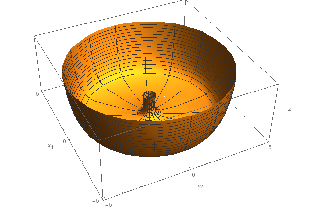
Figure 4: Typical single loop solution (I), left and a double loop solution (II), right.

It is not hard to see that if one imposes a Dirchlet boundary condition in the $z$ direction, then the inner boundary of the hanging string has to ends orthogonally on the D8-brane worldvolume. Namely, in the gauge $z=\sigma$, the Neumann boundary condition in the $\rho$ direction yields

$$\frac{\partial{\mathcal{L}}}{\partial\rho^{\prime}}=\gamma\left(\frac{z_{D4}}{z}\right)^{\frac{3}{2}}\bigg{(}z_{D_{4}}^{3}\rho^{\prime 2}+(zf_{\Lambda})^{-1}\bigg{)}^{-\frac{1}{2}}\rho\rho^{\prime}=0\quad\Rightarrow\quad\frac{{\rm d}\rho}{{\rm d}z}=0\,,$$ (25)

i.e. the string hangs orthogonally from the D8 probe.

For both string configurations, the constituent quark masses are given by Kinar et al. (2000)

$$m_{Q}=\frac{1}{2\pi\alpha^{\prime}}\int_{z_{\Lambda}}^{z_{m_{Q}}}{\rm d}z\,\sqrt{g_{zz}g_{00}}=\frac{1}{2\pi\alpha^{\prime}}\int_{z_{\Lambda}}^{z_{m_{Q}}}{\rm d}z\,\frac{1}{f_{\Lambda}^{1/2}z^{2}}\,,$$ (26)

which is just the proper distance of a string hanging from the tip of the probe D8-brane, $z_{m_{Q}}$ to the IR wall at $z_{\Lambda}$. Note that if there is more than one probe D8-brane, which each ends at a different $z_{{m_{Q}}_{i}}$, then one has a system with different quark masses $m_{Q_{i}}$.

Let us now first look at the solution of type (I). The equation of motion (24) are second order differential equations, and as such have two undetermined constants of integration. In order to see which parameters characterise a solution, let us look at the $z=\sigma$ gauge, since this is the simplest and the results are independent of the gauge. In this gauge $\sigma$ takes values in $(z_{m_{Q}},z_{B})$ where $z_{B}$ is the position of the bottom of the string loop, see figure 6. For the solution (I) we require that the tip of the loop is at the coordinate origin $\rho(z_{B})=0$. Also, as we are interested only in smooth loops, we will require that at the bottom ${\rm d}z/{\rm d}\rho\big{|}_{B}=0$. For a given position of the probe brane $z_{m_{Q}}$, these two requirements uniquely fix the solution (I). We are therefore only left with two parameters which specify the solution (I): $z_{B}$, the position of the bottom of the loop and $z_{m_{Q}}$, specifying the position of the top of the loop. In what follows we will usually work with fixed masses of the outer quarks $m_{Q}$, or equivalently we will fix $z_{m_{Q}}$. If one shifts the bottom of the string $z_{B}$, this will change the distance between the string endpoints, i.e. the distance between the outer quarks $R$ on the probe D8. As the position of the bottom of the loop comes closer to the wall ($z_{B}\rightarrow z_{\Lambda}$) the distance between the quarks $R$ becomes larger and larger, see figure 5.

In this near-wall limit, the single string loop looks more and more like a U-shaped string, see figure 6. Only in this limit $z_{B}\rightarrow z_{\Lambda}$ is the identification of the “vertical” parts of the loop with quark masses 26 fully justified Kinar et al. (2000). Also, only for these kind of U-shaped strings is the effective tension of the horizontal part of the string identified with $\sim\Lambda_{QCD}$, as the position of the wall specifies $\Lambda_{QCD}$ in this model. As the bottom of the loop approaches the IR wall one discovers that the action scales more and more quadratically with the size of the loop, which is the expected behaviour for a single circular Wilson loop in a confining theory.

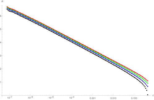
Figure 5: Distance between the quarks (string endpoints) for a single loop $({\bf I})$, as a function of dimensionless separation of the tip of the loop from the wall $\epsilon=(z_{B}-z_{\Lambda})/z_{\Lambda}$. Plots are given for different values of the quark massess: from bottom to top, black $m=1.31$, blue $m=2.03$, green $m=3.55$ and red $m=9.5$.

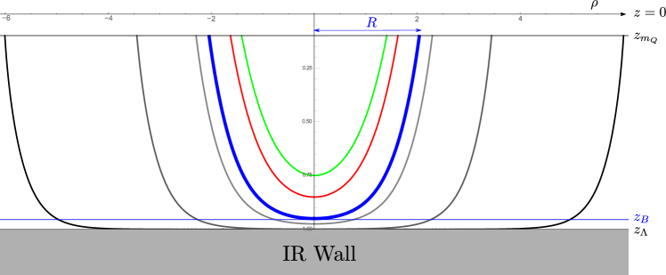
Figure 6: One-parameter family of solutions of type (I) plotted for a mass $m_{Q}=9.57$ of the external quarks. Different solutions are parametrised by different distances between the quarks $R$, or equivalently, different distances from the bottom of the loop to the wall. For all the plots we have set $z_{\Lambda}=1$.

For the double loop solution (${\bf II}$), one needs to introduce two probe D8-branes. The outer boundary of the string worldsheet will end on the brane with position $z=z_{m_{Q}}$. The position of this brane fixes the mass $m_{Q}$ of the original (heavy) quark pair. Before the split, the original flux tube stretches between these two outer quarks. When the flux tube breaks, an inner boundary is formed on the string worldsheet. As argued earlier, the inner boundary of the loop ends orthogonally on the second brane which has position $z=z_{m_{q}}$, and this position fixes the mass of the produced quark-antiquark pair, $m_{q}$. When considering solutions of type (II), we will fix these two parameters $m_{Q}$ and $m_{q}$ as they are the parameters which are given in the dual gauge theory.

Note that the solution (${\bf II}$) consists of two, outer and inner branches, which are glued in a smooth way at the bottom of the loop, $(z_{B},R_{B})$; these are coloured blue and red in figure 7. In contrast to the loop ${\bf(I)}$, the bottom of the loop $({\bf II})$ is no longer at the origin $\rho=0$, but it is placed at some point $(z_{B},\rho=R_{B}\neq 0)$. Smoothness of the solution $({\bf II})$ at the bottom, as before, implies $(dz/d\rho)|_{(z_{B},R_{B})}=0$. In principle, bottom of the loop $z_{B}$ can be anywhere between $0\leq z_{m_{Q}}<z_{m_{q}}<z_{B}\leq z_{\Lambda}$. However, we will be mainly interested in the loops which have bottom near the wall $z_{B}\rightarrow z_{\Lambda}$, since newly generated flux tubes are IR objects which exist at energies $\sim\Lambda_{QCD}$. It is also useful to introduce a dimensionless parameter $\epsilon=(z_{\Lambda}-z_{B})/z_{\Lambda}\ll 1$.

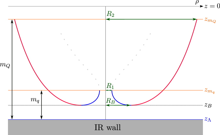
Figure 7: Slice of a generic double loop solution (II) for $\phi=\text{const}$. The labels $z_{m_{Q}}$ and $z_{m_{q}}$ give the positions of two D8-branes and also specify the masses of the original (outer) quarks $m_{Q}$ and pair-produced (inner) quarks $m_{q}$.

Once the bottom of the loop (${\bf II}$) is fixed to some $z=z_{B}$, for a given mass $m_{q}$, the inner (blue) branch of the solution is fully fixed by the requirement of orthogonality of the string to the $m_{q}$ probe brane (see (25)) and the condition of smoothness of the loop at the bottom. Therefore, the radius of the inner loop $R_{1}$ (on the $m_{q}$ brane), as well as the radius $R_{B}$ of the bottom of the loop, are fixed once $z_{B}$ and $m_{q}$ are specified.

The outer (red) branch of the solution is fully fixed once the mass of the original quarks $m_{Q}$ is specified and one requires that this branch is glued in a smooth way to the inner branch. Note that the outer branch of the solution (II) need not end orthogonally on the probe brane $m_{Q}$, as the position of the outer quarks is fixed by Dirichlet boundary conditions. So in summary, solution (II) is fixed by specifying the quark masses $m_{Q}$, $m_{q}$ and the bottom of the loop $z_{B}$, or equivalently, $m_{Q}$, $m_{q}$ and the inner radius $R_{1}$ of the loop.

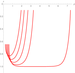
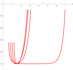
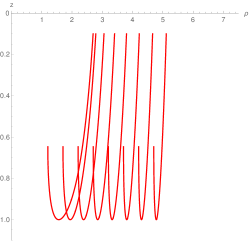
Figure 8: Plots of the loops of type (II) for increasing values of the inner radius $R_{1}$. The left panel shows region (i) until the value for which $R_{2}$ is maximal. The middle panel shows loops in region (ii), where $R_{2}$ decreases as $R_{1}$ increases, until $R_{2}$ reaches its local minimum. The right panel shows the squashed loops of region (iii) which occur beyond that.

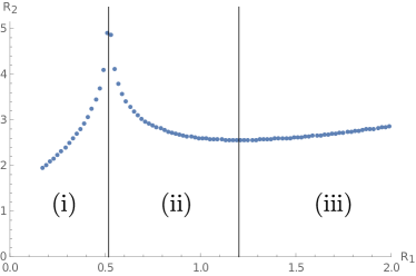
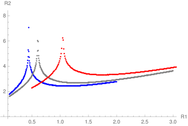
Figure 9: The left panel shows the behaviour of the outer radius as inner radius varies, and the three different regions. Note that there are two critical points on this graph and the “squashing” of loops takes place both in region (ii) and (iii). The right panel shows the behaviour for different masses $m_{q}=\{0.8,1.0,1.5\}$ (blue, gray, red) and fixed mass of the outer quarks $m_{Q}=9.5$.

Let us now try to understand the moduli space of these double loops. First we observe that for fixed $m_{q}$ and $m_{Q}$, as the inner radius $R_{1}$ is increased, the loop extends deeper and deeper into the bulk, towards the IR wall, or in other words, $\epsilon$ decreases. As this happens, initially the loop becomes more and more U-shaped and wider, with increasingly longer horizontal part and with larger and larger outer radius $R_{2}$. In this region, the effective size of the system (the ratio of the outer versus the inner radius) grows. We will refer to this region as region (i). The left panel in figure 8 shows a series of loops in this region. When the inner radius $R_{1}$ becomes larger than a particular critical value $R_{\text{crit-1}}$ the outer radius $R_{2}$ starts to decrease as the inner radius grows, so loops become more and more squashed, see the middle panel in figure 8. Note that while the squashing happens, the bottoms of all the squashed loops stay in the region which is very close to the IR wall ($\epsilon\sim 10^{-5}$). We will refer to this region as region (ii). Finally, when the radius $R_{1}$ becomes larger than another critical value $R_{\text{crit-2}}$, both inner and outer radius start to grow, but the loop retains its squashed shape and it starts moving outwards as a whole; see the right panel in figure 8. We will refer to this as region (iii). Figure 9 shows the relation between the inner and outer radius as the inner radius varies, in all three regions. Note that as the inner quark mass is increased the position of the peak moves to the right, but in a such a way that the ratio of $R_{1}/R_{2}$ increases, so that the the system is effectively at smaller volume. Put differently, systems with smaller inner quark mass $m_{q}$ have larger effective size in the sense discussed above, and we expect them to reproduce the Schwinger results more accurately. The peak in the $R_{2}$ vs. $R_{1}$ plot persists as $m_{q}\rightarrow m_{Q}$, but increasing the masses of outer and inner quarks to larger value reduces the height of the peak and shifts its location to larger values of $R_{1}$, so that eventually, for $m_{q},m_{Q}\rightarrow\infty$, only region (i) remains and one is left with a simple linear relation between $R_{1}$ and $R_{2}$, as expected from e.g. Armoni et al. (2013).

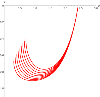
Figure 10: Shapes of double loops (in region (i)) for fixed outer radius $R_{2}=2.4$ and varying inner quark mass. Note that as the inner quark mass decreases, the radius at which these quarks are produced also decreases.

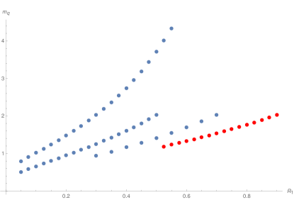
Figure 11: The relation between produced quark mass $m_{q}$ and radius $R_{1}$ at which the pair is produced for various loops in the region (i). The plots are made for $m_{Q}=9.5$ and for different outer radii $R_{2}=\{1.6,1.98,2.37,2.78\}$. The largest value of $R_{2}$ corresponds to the bottom (red) curve.

In order to find the decay width of a given meson, we will need to keep $R_{2}$ and $m_{Q}$ fixed and look at the decay probability for varying inner quark mass $m_{q}$. Figure 10 illustrates that, for strings in region (i), the radius $R_{1}$ at which the inner quarks are produced decreases as $m_{q}$ is decreased. Figure 11 shows the dependence between $m_{q}$ and $R_{1}$ quantitatively, for different values of the outer quark mass $m_{Q}$. It shows that when the total system is smaller ($R_{2}$ is smaller), quarks of the same mass $m_{q}$ are produced at a radius $R_{1}$ which is also smaller. Figure 11 in addition suggests that if $R_{1}\ll R_{2}$ the relation between $R_{1}$ and $m_{q}$ becomes linear, as was the case for the Schwinger approximation (although the slopes of these lines depends on the size of the system, unlike for Schwinger). It is harder, and as we will argue below, less relevant, to produce similar plots for regions (ii) and (iii), as for the “squashed” loops in these regions the dependence of $R_{1}$ on $m_{q}$ is rather weak (small variations of $m_{q}$ lead to almost no change in $R_{1}$).

4.3 Extracting the probability for decay

Once the double loop solution is constructed we want to extract from it the probability for the flux tube to break. As in the case of the flat space instanton 15, in order to compute this probability, one first needs to compute the action of the solution (${\bf II}$) and then subtract from it the action of the action of the solution (${\bf I}$)

$$\Delta S(m_{q},m_{Q},R_{2})=S_{II}(m_{q},m_{Q},R_{2})-S_{I}(m_{Q},R_{2})\,\,.$$ (27)

Both these actions are evaluated for the loops ${\bf(I)}$ and ${\bf(II)}$ which have identical outer radius $R_{2}$, as this corresponds to the physical “size” of the initial system (cf. footnote 4). Generically, the probability for a meson decay will depend on the size of the system $R_{2}$ and on the mass of the initial quarks $m_{Q}$, in addition to the mass of the pair produced quarks $m_{q}$. The dependence of the decay rate on the radius $R_{2}$ is something that one expects for realistic mesons, as the size of a meson is typically related to its angular momentum.

As noted before, for a given system of fixed and large enough $R_{2}$, generically there are three possible radii at which quarks can be pair produced, see figure 9. Each possible radius belongs to one of the regions (i), (ii) or (iii). Let us first analyse instantons in the region (i). Figure 12 shows the instanton action 27 in the region (i) as a function of quark mass. As the quark mass $m_{q}\rightarrow 0$, the instanton action goes to zero, i.e. lighter quarks are more likely to be produced, as expected. We also see that the probability per unit time and volume depends on the “size” of the system, and that the probability for a larger meson to split is smaller than for smaller mesons. This may sounds unintuitive, as one may expect larger mesons to be more unstable. However, one should keep in mind that, when computing the lifetime of mesons, one still needs to multiply this probability with the meson volume.

We should also note that when evaluating the action for instantons using double loops, one always needs to make sure that the instanton action is smaller than the action of two disconnected loops which have the same radii $R_{1}$ and $R_{2}$ Olesen and Zarembo (2000); Gross and Ooguri (1998). For all the loops discussed in this paper, we have always checked that this holds so that no Gross-Ooguri-Olesen-Zarembo type phase transition takes place.

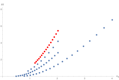
Figure 12: Instanton action as a function of quark mass $m_{q}$, plotted for different size systems $R_{2}=\{1.6,1.98,2.37,2.78\}$. The upper curve (red) with the largest action corresponds to the largest $R_{2}$.

Evaluating the instanton action for radius $R_{1}$ in regions (ii) and (iii) one gets that $S(R_{1\text{(i)}},R_{2})<S(R_{1\text{(ii)}},R_{2})<S(R_{\text{1(iii)}},R_{2})$. We note however, that the difference between these three actions is minimal, less than a percent. Hence it seems that decay in the region (i) is the most dominant, although only marginally. Shapes of generic loops in regions (i), (ii) and (iii) which have the same $R_{2}$ are plotted in figure 13. It is unclear to us at present what is the physical relevance of the squashed loops, in particular the very squashed loops in region (iii). These loops seems to suggest the existence of “exotic” decay channels for meson decay, where the pair-produced quarks remove most of the flux tube in the decay. It could be that, once the treatment of the angular momentum is taken properly into account, these decays are forbidden due to selection rules.

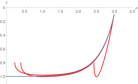
Figure 13: Double loops in the regions (i), (ii) and (iii) for the same outer radius $R_{2}=3.0$ and inner quark mass $m_{q}=0.62$ (corresponding to $z_{m_{q}}=0.8$). The blue curve extending all the way to $\rho=0$ is a single loop with the same radius $R_{2}=3.0$.

So in summary, the computation outlined above produces the probability for the decay of mesons of a particular “size”. It is hard to compare our findings, even at qualitative level, with experimental data, as these are mostly not known for higher spin mesons. However, one expects that in a particular limit, the holographic computation should reproduce to the computations of CNN and Schwinger which were outlined in section 2. Both these computations work with a constant (chromo)electric field in infinite volume and in the approximation where the produced quarks do not back-react on the field.

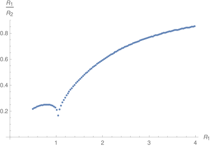
Figure 14: Relative radius $R_{1}/R_{2}$ of the system as a function of the inner radius $R_{1}$ for a fixed chosen mass $m_{1}=1.5$. The largest effective volume is achieved for configurations near the boundary between region (i) and (ii) in the notation of figure 9.

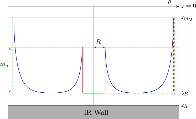
Figure 15: U-shaped loop approximation (red rectangular straight lines for the double loop, green straight lines for the single loop which is to be subtracted). The dashed parts are the same for the single and double loop solutions. For comparison we have also displayed an actual solution (blue curve).

In order to achieve a large-volume limit in the holographic set up, one needs to look at long strings, with a horizontal part which is as large as possible in comparison to the radius $R_{1}$. Figure 14 shows the effective size of the system, i.e. the distance $R_{1}$ at which the quarks are produced versus the full size of the system $R_{2}$ for quarks of fixed mass $m_{q}$. We see that the largest effective volume is achieved for loops at the boundary between the regions (i) and (ii). Note that having the largest effective volume does not mean that the instanton action for these loops is the smallest for a given $m_{q}$ fixed. By looking at shapes of these large-volume loops, see figure 13, we see that they look most stretched and moreover they look most like rectangular U-shaped loops. In order to get an idea of what we should expect the action for these loops to look like in the full numerical solution, let us consider an approximation of these large-volume loops with rectangular U-shaped loops, as indicated in figure 15. In this approximation, the action of the outer part of the loop (the dashed red segments in the figure) is the same for single and double loops and does not contribute to the instanton action. We therefore find that

$$\Delta S_{\text{inst}}\sim S_{\text{tube}}-S_{\text{disc}}\sim 2\pi R_{1}m_{q}-R_{1}^{2}\pi T\,,$$ (28)

where we have used that $m_{q}$ is proportional to the height of the tube, see (26). This expression is similar to the one obtained in the world-line derivation (3), and similar to the flat space expression (15), except that in those expressions the mass $m_{q}$ and the radius $R_{1}$ are linearly related through the equations of motion. In the present case, however, the mass $m_{q}$ and the radius $R_{1}$ are independent since the outer radius is (by construction) decoupled from the rest and is hence arbitrary. Our crude approximation therefore almost, but not completely, reproduces the Schwinger approximation.

Motivated by this discussion, we will now focus attention to strings with the largest possible volume (largest ratio of $R_{1}/R_{2}$), which corresponds to the peak between region (i) and (ii) of figure 8, for small quark mass $m_{q}$. For these strings we find a nice linear relation between $R_{1}$ and $m_{q}$, see figure 16. Note, however, these strings do not all have the same outer radius $R_{2}$. In order to nevertheless compare their actions, we will need to focus only on the inner part of the loop (from $\rho=R_{1}$ to $\rho=R_{B}$). The outer parts of the single and double loop (from $\rho=R_{B}$ to $\rho=R_{2}$) are approximately equal (as they are in the caricature) and would therefore cancel in the instanton action after subtracting the single loop background (see the loop in region (i) in figure 13). As in the caricature, we will furthermore approximate the shape of the single loop between $\rho=0$ and $\rho=R_{B}$ by a straight line segment at constant $z=z_{B}$.

The above is an ‘infinite volume approximation’ in the sense that it holds when $R_{1}\ll R_{2}$. When we plot the instanton action $\Delta S$ versus the produced quark mass $m_{q}$ for these loops, one recovers a quadratic relation, see figure 17. While the best fit is quadratic, like for Schwinger, there is a nonvanishing constant present. One could remove such a term by modifying the normalisation, and it would anyhow be cancelled in a computation of the ratio of any two probabilities, so it is irrelevant. We should also comment that the numerical factor in front of $m_{q}^{2}$ in this fit differs from the factor of $\pi/4$ in the Schwinger/CNN formula (7), which is what one expects. The expression (7) is valid only qualitatively in QCD and also our holographic model is not a dual of real QCD, so one should expect these kind of differences between the two results.

The probability $P_{\text{pp}}$ for a flux tube to break, per unit length and unit time, is obtained by exponentiation of the instanton action. In the approximation of large mesons with an (infinitely long) flux tube, translation invariance implies that the total probability for a meson to split will be given by $P_{\text{pp}}L$, where $L$ is the length of the flux tube. In finite-size systems however, $P_{\text{pp}}$ will in general depend on the position along the flux tube a well as the size of the system. In order to evaluate the full probability we would first need to construct the non-axially symmetric instantons, and then integrate contributions of these instantons over the full length of the flux tube. We leave such an investigation for another project.

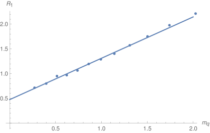
Figure 16: Linear relation between the radius at which quarks are produced and their mass, obtained from the series of “maximal” loops on the boundary between regions (i) and (ii).

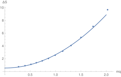
Figure 17: Quadratic dependence of the instanton action $\Delta S$ on the mass $m_{q}$ of the pair-produced quarks in the ‘infinite volume limit approximation’ in which one considers only loops near the boundary between region (i) and (ii).

5 Discussion and outlook

In this paper we have studied decay of mesons using instanton techniques in two models: the old string model and the holographic model of Sakai-Sugimoto. In the first model mesons are represented by a pair of massive particles connected with a relativistic string (flux tube) in flat space. In order to study their decays, we have analytically constructed the worldsheet instanton configuration which interpolates between two mesonic particles. Using this instanton, we were able to reproduce, up to an overall numerical factor, the formula (7) for the probability of breaking the QCD flux tube, derived a long time ago by Casher et al. Casher et al. (1979). They derived their formula by making a direct replacement of various quantities in the QED formula with the analogue quantities in QCD. In contrast, in our approach the connections between the theories followed, rather than being postulated. After comparing the results for the decay probabilities it followed that the chromoelectric field had the same role as an elastic string. However this string does not couple in a minimal way to the massive particles at the string endpoints, unlike the electric or chromo-electric field in the worldline derivation of Schwinger-like formula. Our derivation is very simple, yet it produces quite a non-trivial field theory result. However, it was rudimentary in the sense that we have restricted our attention to planar processes, where both in- and outgoing particles lie in the same plane. It would be interesting to generalise this derivation to allow for the presence of transverse momenta of the outgoing particles.

All of the flat space models (whether Schwinger, CNN or old string) share one “feature”: in order to incorporate (pair production of) quarks one has to introduce an extra term in the action, by hand. In the holographic model, in contrast, there is an unified treatment of the flux tube and quarks. In the second part of the paper we have developed a framework for studying the decay of large-spin mesons using the holographic Sakai-Sugimoto model. We have constructed a family of worldsheet instanton configurations, which interpolates between incoming large-spin meson and two outgoing large-spin mesons. The generic instanton describes the decay in which both the finite size of the system and the backreaction of the pair-produced particles is taken into account. In this sense, the set up is more powerful than either CNN or Schwinger computations which only give the probability in the large volume limit and with no backreaction taken into account. A shortcoming of our computation is that it is restricted to (almost) cylindrically symmetric decay channels. In the infinite volume limit the probability is the same for breaking at all points, but in a finite-size system we expect the probability to be different along the flux tube. It would be very important to study less symmetric decay.

Another restriction of our computation is that the outer (original) quarks were considered only on circular orbits, which is a boundary condition suitable for event generators where quarks accelerate away from each other. In order to compute decays for mesonic particles in general, one would need to generalise our computations to systems in which the external quarks follow straight lines, and construct instantons which are positioned at an arbitrary point along the flux tube. Only than, total decay rates and the life times of the mesonic particles can be computed and one could investigate interesting prediction of the flat space, that $\Gamma/L$ is universal.

When constructing instanton configurations for finite-size mesons, we have discovered an interesting decay channel in which the pair-produced quarks “eat” most of the flux tube, leading to very short outgoing mesons. At the moment it is not clear to us what is the physical significance of such a decay channel. One possibility is that once the angular momentum is properly taken into account (as it is not in our Euclidean framework) these exotic decay channels will be forbidden by a selection rule. It would be interesting to investigate this question in the future. Related to this is the question of proper treatment of angular momentum of mesons in the holographic setup. One expects that angular momentum modifies decay rates, as it provides an extra centrifugal potential for pair-produced quarks. Some of these effects have been investigated for the Schwinger process in Gupta and Rosenzweig (1994).

In order to cross check our computation, we have also investigated meson decays in the large-volume limit. As expected, we have rediscovered the qualitative form of the Schwinger/CNN formula, up to a numerical factor. The long strings which were used in this large-volume limit offer a natural playground in which one could try to set up a systematic study of finite-size effects. Namely, for large, but finite-size systems, the probability for a string to decay should have an expansion in powers of $R_{1}/R_{2}$, where $R_{1}$ is the radius at which quarks are produced and $R_{2}$ is the size of the system. It would be interesting to quantitatively study this expansion using the holographic set up.

It would also be interesting to extend our analysis to finite temperature field theory. By introducing a horizon in the Sakai-Sugimoto setup one could generalise our instanton configuration to this background, and obtain the thermal probability for a flux tube to split. Finally, one could ask to which extend the results which we obtain are dependent on the exact form of the metric. In particular, one might ask if for instantons in other confining geometries the quadratic dependence on the quark mass persists. We plan to investigate these issues in future work.

References

- Sakai and Sugimoto (2006) T. Sakai and S. Sugimoto, “More on a holographic dual of QCD”, Prog. Theor. Phys. 114 (2006) 1083–1118, hep-th/0507073.
- Sjöstrand (1982) T. Sjöstrand, “The Lund Monte Carlo for jet fragmentation”, Comp. Phys. Commun. 27 (1982) 243.
- Andersson et al. (1983) B. Andersson, G. Gustafson, G. Ingelman, and T. Sjöstrand, “Parton fragmentation and string dynamics”, Phys. Rep. 97 (1983) 31.
- Casher et al. (1979) A. Casher, H. Neuberger, and S. Nussinov, “Chromoelectric flux tube model of particle production”, Phys. Rev. D20 (1979) 179–188.
- Armoni (2008) A. Armoni, “Beyond The Quenched (or Probe Brane) Approximation in Lattice (or Holographic) QCD”, Phys. Rev. D78 (2008) 065017, arXiv:0805.1339.
- Peeters et al. (2006) K. Peeters, J. Sonnenschein, and M. Zamaklar, “Holographic decays of large-spin mesons”, JHEP 02 (2006) 009, hep-th/0511044.
- Sonnenschein and Weissman (2018) J. Sonnenschein and D. Weissman, “The decay width of stringy hadrons”, Nucl. Phys. B927 (2018) 368–454, arXiv:1705.10329.
- Affleck et al. (1982) I. K. Affleck, O. Alvarez, and N. S. Manton, “Pair Production at Strong Coupling in Weak External Fields”, Nucl. Phys. B197 (1982) 509–519.
- Schwinger (1951) J. S. Schwinger, “On gauge invariance and vacuum polarization”, Phys. Rev. 82 (1951) 664–679.
- Affleck and Manton (1982) I. K. Affleck and N. S. Manton, “Monopole Pair Production in a Magnetic Field”, Nucl. Phys. B194 (1982) 38–64.
- Nayak (2005) G. C. Nayak, “Non-perturbative quark-antiquark production from a constant chromo-electric field via the Schwinger mechanism”, hep-ph/0510052.
- Barbashov and Nesterenko (1990) B. M. Barbashov and V. V. Nesterenko, “Introduction to the relativistic string theory”, 1990.
- Semenoff and Zarembo (2011) G. W. Semenoff and K. Zarembo, “Holographic Schwinger Effect”, Phys. Rev. Lett. 107 (2011) 171601, arXiv:1109.2920.
- Bardeen et al. (1976) W. A. Bardeen, I. Bars, A. J. Hanson, and R. D. Peccei, “A study of the longitudinal kink modes of the string”, Phys. Rev. D13 (1976) 2364–2382.
- Kruczenski et al. (2005) M. Kruczenski, L. A. P. Zayas, J. Sonnenschein, and D. Vaman, “Regge trajectories for mesons in the holographic dual of large- QCD”, JHEP 06 (2005) 046, hep-th/0410035.
- Kinar et al. (2000) Y. Kinar, E. Schreiber, and J. Sonnenschein, “ potential from strings in curved spacetime – classical results”, Nucl. Phys. B566 (2000) 103–125, hep-th/9811192.
- Armoni et al. (2013) A. Armoni, M. Piai, and A. Teimouri, “Correlators of Circular Wilson Loops from Holography”, Phys. Rev. D88 (2013), no. 6, 066008, arXiv:1307.7773.
- Olesen and Zarembo (2000) P. Olesen and K. Zarembo, “Phase transition in Wilson loop correlator from AdS / CFT correspondence”, arXiv:hep-th/0009210.
- Gross and Ooguri (1998) D. J. Gross and H. Ooguri, “Aspects of large N gauge theory dynamics as seen by string theory”, Phys. Rev. D58 (1998) 106002, arXiv:hep-th/9805129.
- Gupta and Rosenzweig (1994) K. S. Gupta and C. Rosenzweig, “Semiclassical decay of excited string states on leading regge trajectories”, Phys. Rev. D50 (1994) 3368–3376, hep-ph/9402263.