A particle-based variational approach to Bayesian Non-negative Matrix Factorization

Abstract

Bayesian Non-negative Matrix Factorization (NMF) is a promising approach for understanding uncertainty and structure in matrix data. However, a large volume of applied work optimizes traditional non-Bayesian NMF objectives that fail to provide a principled understanding of the non-identifiability inherent in NMF– an issue ideally addressed by a Bayesian approach. Despite their suitability, current Bayesian NMF approaches have failed to gain popularity in an applied setting; they sacrifice flexibility in modeling for tractable computation, tend to get stuck in local modes, and require many thousands of samples for meaningful uncertainty estimates. We address these issues through a particle-based variational approach to Bayesian NMF that only requires the joint likelihood to be differentiable for tractability, uses a novel initialization technique to identify multiple modes in the posterior, and allows domain experts to inspect a ‘small’ set of factorizations that faithfully represent the posterior. We introduce and employ a class of likelihood and prior distributions for NMF that formulate a Bayesian model using popular non-Bayesian NMF objectives. On several real datasets, we obtain better particle approximations to the Bayesian NMF posterior in less time than baselines and demonstrate the significant role that multimodality plays in NMF-related tasks.

1 Introduction

The goal of non-negative matrix factorization (NMF) is to find a rank-$R$ factorization for a non-negative data matrix $X$ ($D$ dimensions by $N$ observations) into two non-negative factor matrices $A$ and $W$. Typically, the rank $R$ is much smaller than the dimensions and observations ($R\ll D,N$).

$$X\approx AW\quad|\quad\quad X\in\mathbb{R}_{+}^{D\times N},\quad A\in\mathbb{R}_{+}^{D\times R},\quad W\in\mathbb{R}_{+}^{R\times N}$$

The linear additive structure of these non-negative factor matrices makes NMF a popular unsupervised learning framework for discovering and interpreting latent structure in data. Each observation in the data $X$ is approximated by an additive combination of the $R$ columns of $A$ with the combination weights given by the column of $W$ corresponding to that observation. In this way, the basis matrix $A$ provides a part-based representation of the data and the weights matrix $W$ provides an $R$-dimensional latent representation of the data under this part-based representation.

Applications of NMF include understanding protein-protein interactions (Greene et al., 2008), topic modeling (Roberts et al., 2016), hyperspectral unmixing (Bioucas-Dias et al., 2012), polyphonic music transcription (Smaragdis and Brown, 2003), discovering molecular pathways from genomic samples (Brunet et al., 2004), and summarizing activations of a neural network for greater interpretretability (Olah et al., 2018).

NMF is known to be a difficult problem: in the absence of noise, NMF is NP-hard (Vavasis, 2009) and NMF objectives in general are non-convex. In addition, analysis and interpretation of latent structure in a dataset via NMF is affected by the the possibility that several non-trivially different pairs of $A,W$ may reconstruct the data $X$ equally well. This non-identifiability of the NMF solution space has been studied in detail in the theoretical literature (Pan and Doshi-Velez, 2016; Donoho and Stodden, 2003; Arora et al., 2012; Ge and Zou, 2015b; Bhattacharyya et al., 2016), and is of practical concern as well. Greene et al. (2008) use ensembles of NMF solutions to model chemical interactions, while Roberts et al. (2016) conduct a detailed empirical study of multiple optima in the context of extracting topics from large corpora.

Bayesian approaches to NMF promise to characterize this parameter uncertainty in a principled manner by solving for the posterior $p(A,W|X)$ given priors $p(A)$ and $p(W)$ and likelihood $p(X|A,W)$ e.g. Schmidt et al. (2009); Moussaoui et al. (2006). Having a representation of uncertainty in the parameters of the factorizations can assist with the proper interpretation of the factors, allowing us to place low or high confidence on parameters of the factorization. However, computational tractability of inference in Bayesian models is a concern that limits the application of the Bayesian approach. Additionally, the uncertainty estimates obtained from current Bayesian methods are often of limited use: variational approaches (e.g. Paisley et al. (2015); Hoffman and Blei (2015)) typically underestimate uncertainty and fit to a single mode; sampling-based approaches (e.g. Schmidt et al. (2009); Moussaoui et al. (2006)) also rarely switch between multiple modes and require many thousands of samples for meaningful uncertainty estimates.

As a result of the limitations of current Bayesian approaches, practitioners tend to rely on non-Bayesian approaches to understand structure in matrix data and explore uncertainty in NMF parameters. For example, Greene et al. (2008); Roberts et al. (2016); Brunet et al. (2004) use random restarts to find multiple solutions. Random restarts have no Bayesian interpretation (depending on the basins of attraction of each mode), but they do often find multiple optima in the objective that can be used to understand and interpret the data. Despite its usefulness, the random restarts approach lacks the principled nature of a Bayesian treatment.

We introduce a Bayesian NMF framework that incorporates the benefits of non-Bayesian approaches into the principled Bayesian context by constructing a discrete distribution over the space of factorizations where the probability masses are optimized under the Stein variational objective (Ranganath et al., 2016). In addition, we provide a novel initialization strategy for NMF that uses transfer learning to provide high-quality and diverse initializations for NMF that reduce optimization time for NMF algorithms and find multiple optima in the NMF objective. Finally, this work also introduces a class of likelihood and prior models for Bayesian NMF that easily allow practitioners to re-formulate their problems (using traditional non-Bayesian NMF objectives) as Bayesian. Once the Bayesian model is chosen, a set of factorizations from high-likelihood regions of the posterior are found by combining our novel initialization technique with state-of-the-art non-Bayesian NMF algorithms. Subsequently, probability masses are assigned to each factorization such that the divergence from the posterior as measured by the Stein variational objective is minimized.

We demonstrate through multiple real datasets that:

• Our particle-based posterior approximation framework consistently outperforms baselines in terms of approximation quality and runtime.

• Our framework produces diverse sets of particles from multiple modes of the posterior landscape that have distinct interpretations, exhibit variability in performance on downstream tasks, and improve user ability to inspect and understand the full solution space.

2 Inference Setting

We seek to approximate the Bayesian NMF posterior $p(\theta|X)$ with a discrete variational distribution $q(\theta|\theta_{1:M},w_{1:M})$ that has $M$ different point-masses $\theta_{m}$. Each $\theta_{m}$ represents a different NMF solution’s full set of parameters: $\theta_{m}=\{A_{m},W_{m}\}$, and is assigned probability mass $w_{m}$. The functional form of the variational distribution is given by:

$$\begin{split}p(\theta|X)&\approx q(\theta|\theta_{1:M},w_{1:M})=\sum_{m=1}^{M}w_{m}\delta(\theta-\theta_{m})\quad\\ &s.t\quad w_{1:M}\in\Delta^{M-1},\quad\text{where}\quad\theta_{m}=\text{vec}[A_{m}^{T},W_{m}]\end{split}$$ (1)

where $\delta$ is the Dirac delta distribution and $\Delta^{M-1}$ is the probability simplex in $\mathbb{R}^{M}$. The task of effectively constructing this discrete approximation depends on producing high-quality, diverse factorization collections $\theta_{1:M}$ and determining their associated weights $w_{1:M}$.

The approximation quality between the discrete distribution $q(\theta|\theta_{1:M},w_{1:M})$ and the posterior distribution $p(\theta|X)$ of interest can be quantified using recent advances in Stein discrepancy evaluation with kernels (Liu and Feng, 2016; Chwialkowski et al., 2016; Gretton et al., 2006; Liu et al., 2016; Gorham and Mackey, 2015). While the popular Kulback-Leibler divergence requires comparing the ratio of probability densities or probability masses, the Stein discrepancy can be used to compare a particle-based collection defined by probability masses with a continuous target distribution. Equation 2 summarizes the objective of our particle-based variational approach: we minimize the Stein discrepancy $\mathbb{S}_{p}(q)$ with respect to the Bayesian NMF posterior $p(\theta|X)$ of a discrete variational distribution $q(\theta|\theta_{1:M},w_{1:M})$. In Section 4, we introduce our main algorithm to solve this objective efficiently (Algorithm 1).

$$q^{*}(\theta|\theta_{1:M},w_{1:M})=\text{argmin}_{\theta_{1:M},w_{1:M}}\mathbb{S}_{p(\theta|X)}(q(\theta|\theta_{1:M},w_{1:M}))\quad s.t.\quad w_{1:M}\in\Delta^{M-1}$$ (2)

3 Background

Bayesian Non-negative Matrix Factorization

In Bayesian NMF, we define priors $p(A)$ and $p(W)$ and a likelihood $p(X|A,W)$ and seek to characterize the posterior $p(A,W|X)$. These are related by Bayes’ rule:

$$p(A,W|X)=\frac{p(X|A,W)p(A)p(W)}{p(X)}$$

There exist many options for the choice of prior and likelihood (e.g., exponential-Gaussian, (Paisley et al., 2015; Schmidt et al., 2009), Gamma Markov chain priors (Dikmen and Cemgil, 2009) and volume-based priors (Arngren et al., 2011)). The likelihood and prior choices are often sought in order to have good computational properties (e.g. the resulting partial conjugacy of exponential-Gaussian model). One feature of our work is that we do not require convenient priors for the inference task.

Transfer Learning

The field of transfer learning aims to leverage models and inference applied to one problem to assist in solving related problems. It is of practical value because there may be an abundance of data and computational resources for one problem but not another (see Pan and Yang (2010) for a survey). In this work, we shall use the solutions to Bayesian NMF from small, synthetic problems to quickly solve much larger NMF problems.

Stein discrepancy

The Stein discrepancy $\mathbb{S}_{p}(q)$ is a divergence from distributions $q(\theta)$ to $p(\theta)$ that only requires sampling from the variational distribution $q(\theta)$ and evaluating the score function of the target distribution $p(\theta)$. The Stein discrepancy is computed over some class of test functions $f\in\mathcal{F}$ and satisfies the closeness property for operator variational inference (Ranganath et al., 2016): it is non-negative in general and zero only for some equivalence class of distributions $q\in\mathcal{Q}_{0}$. For a rich enough function class, the only distribution for which the Stein discrepancy is zero is the distribution $p$ itself. The approximation quality between the discrete distribution $q(\theta|\theta_{1:M},w_{1:M})$ and the posterior distribution $p(\theta|X)$ of interest can be analytically computed using recent advances in Stein discrepancy evaluation with kernels (Liu and Feng, 2016; Chwialkowski et al., 2016; Gretton et al., 2006; Liu et al., 2016; Gorham and Mackey, 2015). The Stein discrepancy is related to the maximum mean discrepancy (MMD): a discrepancy that measures the worst-case deviation between expectations of functions $h\in\mathcal{H}$ under $p$ and $q$ (Gretton et al., 2006).

$$\text{MMD}(\mathcal{H},q,p):=\sup_{h\in\mathcal{H}}\mathbb{E}_{\theta\sim q}h(\theta)-\mathbb{E}_{\theta^{\prime}\sim p}h(\theta^{\prime})$$

By applying the Stein operator $\mathcal{T}_{p}$ corresponding to the distribution $p$, the function space $\mathcal{H}$ is transformed into another function space $\mathcal{T}_{p}(\mathcal{H})=\mathcal{F}$. Expectations under $p$ of any $f\in\mathcal{F}$ are zero, i.e. $\mathbb{E}_{\theta^{\prime}\sim p}f(\theta^{\prime}))=0$. This property of the Stein operator is of particular interest when the distribution $p$ is intractable because evaluating the Stein discrepancy does not require expectations over $p$ and the Stein operator $\mathcal{T}_{p}$ only depends on the unnormalized distribution via the score function $\nabla_{\theta}\log p(\theta)$.

$$\mathbb{S}_{p}(\mathcal{H},q):=\sup_{f\in\mathcal{T}_{p}(\mathcal{H})}(\mathbb{E}_{\theta\sim q}f(\theta))^{2}$$

In this work, we use a kernalized form of the Stein discrepancy. For every positive definite kernel $k(\theta,\theta^{\prime})$, a unique Reproducing Kernel Hilbert Space (RKHS) $\mathcal{H}$ is defined. Chwialkowski et al. (2016) showed that the Stein operator applied to an RKHS defines a modified positive definite kernel $\mathcal{K}_{p}$ given by:

$$\begin{split}\mathcal{K}_{p}(\theta,\theta^{\prime})&=\nabla_{\theta}\log p(\theta)^{T}\nabla_{\theta^{\prime}}\log p(\theta^{\prime})k(\theta,\theta^{\prime})\\ &+\nabla_{\theta^{\prime}}\log p(\theta^{\prime})^{T}\nabla_{\theta}k(\theta,\theta^{\prime})\\ &+\nabla_{\theta}\log p(\theta)^{T}\nabla_{\theta^{\prime}}k(\theta,\theta^{\prime})\\ &+\sum_{i=1}^{d}\frac{\partial^{2}k(\theta,\theta^{\prime})}{\partial\theta_{i}\partial\theta^{\prime}_{i}}\end{split}$$ (3)

Finally, the Stein discrepancy is simply the expectation of the modified kernel $\mathcal{K}_{p}$ under the joint distribution of two independent variables $\theta$, $\theta^{\prime}\sim q$.

$$\mathbb{S}_{p}(q)=\mathbb{E}_{\theta,\theta^{\prime}\sim q}\mathcal{K}_{p}(\theta,\theta^{\prime})$$

For a discrete distribution over $\theta_{1:M}$ with probability masses $w_{1:M}$ (of the form in equation 1), this can be evaluated exactly (Liu and Lee, 2016) as:

$$\begin{split}\mathbb{S}_{p}(q)&=\sum_{i,j=1}^{M}w_{i}w_{j}\mathcal{K}_{p}(\theta_{i},\theta_{j})\\ &=\mathbf{w}^{T}\mathbf{K}\mathbf{w}\\ \end{split}$$ (4)

The (pure) quadratic form $\mathbf{w}^{T}\mathbf{K}\mathbf{w}$ is a reformulation where $\mathbf{K}\in\mathbb{R}^{M\times M}$ is the (positive definite) pairwise kernel matrix with entries $\mathbf{K}_{ij}=\mathcal{K}_{p}(\theta_{i},\theta_{j})$ and the probability masses $w_{1:M}$ are embedded into a vector $\mathbf{w}\in\mathbb{R}^{M\times 1}$. Our particle-based variational objective (equation 2) simplifies to the form in equation 4. In Section  4, we will provide a method for estimating $\theta_{1:M}$ and $w_{1:M}$ for the Bayesian NMF problem.

4 Approach

In this section, we present a procedure to approximate the Bayesian NMF posterior with a discrete distribution over factorizations $\theta_{1:M}$ (summarized in Algorithm 1). NMFs $\theta_{1:M}$ are found by running state-of-the-art (non-Bayesian) algorithms that are initialized using our novel transfer-based technique (Section 4.1). Given $\theta_{1:M}$, we apply out of the box convex optimization tools to find the optimal weights $w_{1:M}$ for representing the posterior i.e. minimize Stein discrepancy.

4.1 Learning factorization parameters $\theta_{1:M}$ via Transfer Learning

A natural approach to finding the factorization parameters $\theta_{1:M}$ is to optimize for them directly via the variational objective (equation 4), but we demonstrate this approach suffers from getting stuck in poor local optima and prohibitive computational requirements (see Section 7). Since the quality of the variational approximation is determined solely by the value of the variational objective under a given set of parameters $\theta_{1:M}$, $w_{1:M}$, we are free to employ any technique that produces a suitable collection $\theta_{1:M}$.

To explore multi-modal spaces (such as the Bayesian NMF posterior), random restart-based approaches are known to introduce diversification to overcome the problem of converging to a single local mode (Gendreau and Potvin, 2010). Specialized (non-Bayesian) optimization algorithms for NMF (Lee and Seung, 2001; Lin, 2007; Hsieh and Dhillon, 2011) are widely used in applied settings to produce single factorization parameters $\theta_{m}$. Since the convergence of these algorithms is dependent on initializations, random restarts can be used to discover multiple modes. That said, random restarts compound computational concerns related to the slow convergence rates of many (non-Bayesian) NMF algorithms—hence also a literature for initializations that can speed up convergence (Salakhutdinov et al. (2002), Wild et al. (2004), Xue et al. (2008), Boutsidis and Gallopoulos (2008)).

In this section, we introduce an initialization technique (which we will call $Q$-Transform) to speed-up, as compared to random restarts, the process of finding a diverse set of factorizations from high-density regions of the posterior. Initializations are determined by transforming the low-rank subspace of the singular value decomposition (SVD) using transformation matrices discovered via synthetic datasets. Figure 1 shows a schematic illustrating the idea that transformation matrices $Q_{A},Q_{W}$ generated from one dataset can be applied to another dataset. In the context of this work, we repeatedly apply NMF algorithms to obtain a collection of diverse NMFs. The overall speedup due to $Q$-Transform is equal to the time advantage due to a single $Q$-Transform initialization, multiplied by the number of factorizations we compute ($M$). To explain our $Q$-Transform procedure, we first define the subspace transformation matrices, then describe the method for generating transformation matrices $Q_{A},Q_{W}$ using synthetic data, and applying them to real data sets (transfer learning).

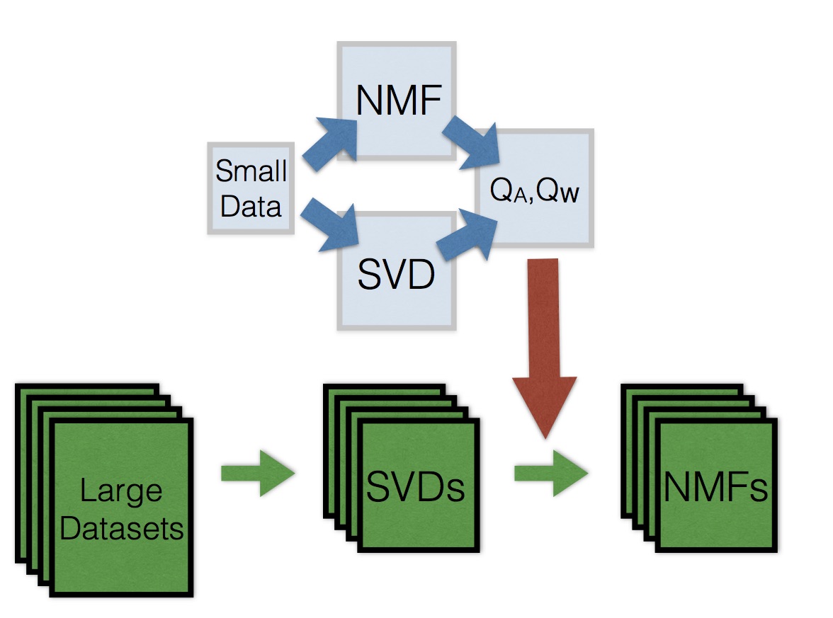
Figure 1: A schematic of the transfer learning procedure for NMF: A small dataset is used to learn transformation matrices $Q_{A},Q_{W}$. We then apply these transformation matrices to multiple larger datasets (with any number of dimensions or observations) using its SVD to obtain a transfer-based initialization.

Algorithm 1 Particle-based Variational Inference for Bayesian NMF using $Q$-Transform

  Input: Data $\{X\}$, Rank $\{R_{\text{NMF}}\}$, # Factorizations $M$

  Step 1: Perform $M$ repetitions of Algorithm 2 to get matrices $\{Q_{A}^{m},Q_{W}^{m}\}_{m=1}^{M}$ or re-use them if previously constructed

  Step 2: Apply $Q$-Transform (Algorithm 3) to get Initializations $\{A_{0}^{m},W_{0}^{m}\}_{m=1}^{M}$

  Step 3: Apply NMF algorithm to get Factorizations $\{A^{m},W^{m}\}_{m=1}^{M}$

  Step 4: Apply Algorithm 5 using a given Bayesian NMF model to get weights $\{w^{m}\}_{m=1}^{M}$ for approximate posterior

  Output: Discrete NMF Posterior $\{w^{m},A^{m},W^{m}\}_{m=1}^{M}$

Subspace Transformations $Q_{A},Q_{W}$ relating SVD and NMF.

A low dimensional approximation for the data $X$ can be obtained via the top $R_{\text{SVD}}$ vectors of the SVD $A_{\text{SVD}},W_{\text{SVD}}$. An NMF $A,W$ of rank $R_{T}$ (which may be different from $R_{\text{SVD}}$) also leads to an approximation of the data. The NMF factors are interpretable due to the non-negativity constraint whereas the SVD factors typically violate non-negativity. However, both approaches describe low dimensional subspaces that can be used to understand and approximate the data. These subspaces are the same when $R_{\text{SVD}}=R_{T}$ and the NMF is exact (i.e. $X=AW$; corresponds to Type I non-identifiability in Pan and Doshi-Velez (2016)). Under these conditions, there exist transformation matrices $Q_{A},Q_{W}$ to obtain the non-negative basis and weights in terms of the singular value decomposition matrices:

$$\begin{split}\text{If}\quad X=A_{\text{SVD}}W_{\text{SVD}}=AW\quad\text{then}\\ A=A_{\text{SVD}}Q_{A}\quad W=Q_{W}W_{\text{SVD}}\end{split}$$

When these conditions are not met, we may still expect the subspaces to be similar and expect that there exist transformation matrices $Q_{A}\in\mathbb{R}^{R_{\text{SVD}}\times R_{T}},Q_{W}\in\mathbb{R}^{R_{T}\times R_{\text{SVD}}}$ to yield approximations of the NMF factorizations.

$$A_{Q}=A_{\text{SVD}}Q_{A}\approx A\quad W_{Q}=Q_{W}W_{\text{SVD}}\approx W$$

The matrices $A_{Q}\in\mathbb{R}^{D\times R_{T}},W_{Q}\in\mathbb{R}^{R_{T}\times N}$ approximate the NMF matrices but adjustments may be required to ensure the dimensions are equal to those of the factorization sought, and that the entries are non-negative before they can be used as an initialization $A_{0},W_{0}$ (see Algorithm 4).

Application of Transformations $Q_{A},Q_{W}$ for NMF Initialization:

If we have already computed an NMF $A,W$ for a dataset $X$, appropriate transforms $Q_{A},Q_{W}$ can be computed by relating the SVD factors $A_{\text{SVD}},W_{\text{SVD}}$ to $A,W$ (e.g. via linear least squares). This approach gives useful transformation matrices but provides no advantage since the NMF has already been computed. However, if we have a set of $Q_{A},Q_{W}$ from one dataset, can we use them for another?

In the following, we shall generate these transforms using random restarts on small, synthetic datasets $X_{s}$ that follow some generative model for NMF, where we can run NMF algorithms quickly and solve for $Q_{A},Q_{W}$ (Algorithm 2). Multiple pairs of transformation matrices can be obtained by repeating Algorithm 2 with different random initializations to compute NMF of the synthetic data $X_{s}$, or by generating new synthetic datasets. We find that knowledge from these transformations $Q_{A},Q_{W}$ can be transferred to real datasets by re-using them to relate the top SVD factors of other datasets to high quality, approximately non-negative factorizations. Since the transformations $Q_{A},Q_{W}$ act on the inner dimensions (columns of $A_{\text{SVD}}$ and rows of $W_{\text{SVD}}$), we emphasize that they can be applied to new datasets with any number of dimensions $D$ and number of observations $N$. Given the top SVD factors of a new dataset $A_{\text{SVD}},W_{\text{SVD}}$, we apply the $Q$-Transform (Algorithm 3) which multiplies SVD factors by the $Q_{A},Q_{W}$ matrices and adjusts entries of $A_{\text{SVD}}Q_{A}$ and $Q_{W}W_{\text{SVD}}$ using Algorithm 4 to obtain initializations $A_{0},W_{0}$ that can be used for any standard NMF algorithm (e.g. Cichocki and Phan (2009), Févotte and Idier (2011)) to give us factorization parameters $\theta_{m}=\text{vec}[A_{m}^{T},W_{m}]$.

We provide a publicly available demonstration of Algorithms 2 and  3 in python to show the effectiveness of the $Q$-Transform initializations.

Algorithm 2 Generate $Q$-Transform Matrices

  Input: Synthetic Data $\{X_{s}\}$, SVD Dimension $\{R_{\text{SVD}}\}$, Transfer Dimension $\{R_{T}\}$

  $A_{\text{SVD}},W_{\text{SVD}}$ $\leftarrow$ Compute top $R_{\text{SVD}}$ SVD of $X_{s}$

  $A_{\text{NMF}},W_{\text{NMF}}$ $\leftarrow$ Compute rank-$R_{T}$ NMF of $X_{s}$ using random initialization

  $Q_{A}=\underset{Q}{\operatorname{arg}\,\operatorname{min}}\;\|A_{\text{NMF}}-A_{\text{SVD}}Q\|_{F}$ via linear least squares

  $Q_{W}=\underset{Q}{\operatorname{arg}\,\operatorname{min}}\;\|W_{\text{NMF}}-QW_{\text{SVD}}\|_{F}$ via linear least squares

  Output: $Q_{A}$, $Q_{W}$

Algorithm 3 Apply $Q$-Transform

  Input: Real Data $\{X\}$, SVD Rank $\{R_{\text{SVD}}\}$, NMF Rank $\{R_{\text{NMF}}\}$, Transformation Matrices $\{Q_{A},Q_{W}\}$

  $A_{\text{SVD}},W_{\text{SVD}}$ $\leftarrow$ Compute top $R_{\text{SVD}}$ SVD of $X$

  $A_{0},W_{0}\leftarrow\text{Initialization Adjustment}(A_{\text{SVD}}Q_{A},Q_{W}W_{\text{SVD}},R_{\text{NMF}})$

  Output: $A_{0}$, $W_{0}$

Algorithm 4 Initialization Adjustment

  Input: Approximation matrices $\{A_{Q},W_{Q}\}$, NMF Rank $\{R_{\text{NMF}}\}$

  $\tilde{A_{0}}\leftarrow\text{Absolute Value}(A_{Q})$

  $\tilde{W_{0}}\leftarrow\text{Absolute Value}(W_{Q})$

  Transfer Rank $R_{T}$ = $\#$ Columns of $A_{Q}$

  if NMF Rank $R_{\text{NMF}}>$ Transfer Rank $R_{T}$ then

     $r=R_{\text{NMF}}-R_{T}$

     Pad $\tilde{A_{0}},\tilde{W_{0}}$ with matrices $M_{D\times r}$ and $M_{N\times r}$ having small random entries so that initializations are the correct dimensions and matrices $M_{D\times r},M_{N\times r}$ have little effect of the product $\tilde{A_{0}}\tilde{W_{0}}$.

     $A_{0}\leftarrow[\tilde{A_{0}},M_{D\times k}]$

     $W_{0}\leftarrow[\tilde{W_{0}}^{T},M_{N\times k}]^{T}$

  else if NMF Rank $R_{\text{NMF}}<$ Transfer Rank $R_{T}$ then

     Pick the top $R_{\text{NMF}}$ columns of $\tilde{A_{0}}$ and rows of $\tilde{W_{0}}$

     $A_{0}\leftarrow\tilde{A_{0}}[:,0:R_{\text{NMF}}]$

     $W_{0}\leftarrow\tilde{W_{0}}[0:R_{\text{NMF}},:]$

  end if

4.2 Learning weights $w_{1:M}$ given parameters $\theta_{1:M}$

To infer the weights corresponding to a given factorization collection $\theta_{1:M}$, we minimize the Stein discrepancy (Algorithm 5) subject to the simplex constraint on the weights. This process involves first computing the pairwise kernel matrix $\mathbf{K}$ using the kernel $\mathcal{K}_{p}$ in equation 3. The objective function is convex and can be solved using standard convex optimization solvers. Given point-masses $\theta_{1:M}$, this framework can be employed to infer weights for discrete approximations to any posterior for which the score function $\nabla_{\theta}\log p(\theta)$ can be computed.

Algorithm 5 Kernalized Stein inference for discrete approximations to posterior

  Input: Particles $\theta_{1:M}$, Score $\nabla_{\theta}\log p(\theta)$, RKHS $\mathcal{H}$ defined by kernel $k$

  Step 1: Compute pairwise kernel matrix $\mathbf{K_{i,j}}=\mathcal{K}_{p}(\theta_{i},\theta_{j})$ (from equation 3)

  Step 2: Find probability masses that minimize the Stein discrepancy for the given point-masses: $\mathbf{w^{*}}=\arg\min_{\mathbf{w}}\mathbf{w}^{T}\mathbf{K}\mathbf{w}\quad\text{s.t}\quad\mathbf{w}\in\Delta^{M-1}$ via standard convex optimization.

  Output: Probability masses $\mathbf{w^{*}}$

5 Threshold-based Bayesian NMF Model

The procedure described in Algorithm 1 for finding a discrete approximation to the Bayesian NMF posterior does not depend on any special properties (such as conjugacy) and only requires the joint density $p(X,W,A)$ to be differentiable in order to make inference tractable. In the following, we take advantage of this added freedom to consider a class of models that correspond to what practitioners are directly concerned with. The purpose of this class of models is to allow practitioners to take any application-specific notion of a high-quality factorization and put it into a Bayesian context.

The ability to incorporate application-specific notions of factorization quality is valuable because notions vary. Squared Euclidean distance is used in hyperspectral unmixing (Bioucas-Dias et al., 2012), Kullback-Leibler divergence in image analysis (Lee and Seung, 2001) and Itakura-Saito divergence for music analysis (Févotte et al., 2009). Roberts et al. (2016) notes that these objectives typically only approximate factorization quality, and so, practitioners may be equally interested in all factorizations that meet some quality criteria defined by the the objective. In the Bayesian NMF setting, we would like to construct likelihood models that reflect these application-specific preferences of practitioners.

5.1 Likelihood: Soft Insensitive Loss Function (SILF) over NMF objectives

We define a likelihood that is maximum (and flat) in the region of high quality factorizations and decays as factorization quality decreases. To do so, we use the soft insensitive loss function (SILF) (Chu et al., 2004): a loss function defined over the real numbers $\mathbb{R}$, where the loss is negligible in some region around zero defined by the insensitivity threshold $\epsilon$, and grows linearly outside that region (see figure 2). A quadratic term depending on the smoothness parameter $\beta$, makes the transition between the two main regions smooth. This transition region has length $2\beta$, making smaller values of $\beta$ correspond to sharper transitions between the flat and linear loss regions. We adapt the SILF from (Chu et al., 2004) to only be defined over the non-negative numbers $\mathbb{R}_{+}$ (as is typical with NMF objectives) and define it as:

$$\text{SILF}_{\epsilon,\beta}(y)=\left\{\begin{array}[]{ll}0&\quad 0\leq y\leq(1-\beta)\epsilon\\ \frac{(y-(1-\beta))^{2}}{4\beta\epsilon}&\quad(1-\beta)\epsilon\leq y\leq(1+\beta)\epsilon\\ y-\epsilon&\quad y\geq(1+\beta)\epsilon\end{array}\right.$$

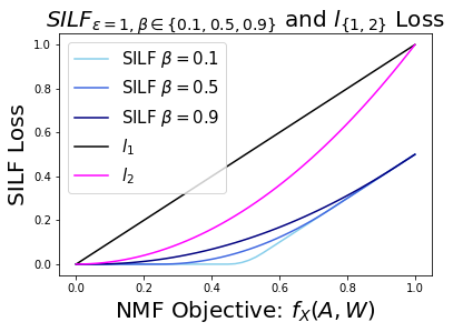
Figure 2: A comparison of SILF loss and commonly used $l_{1},l_{2}$ loss functions. The SILF insensitivity parameter $\epsilon$ is set to 0.5, and the smooth transition factor $\beta$ is varied. Small values of $\beta$ lead to sharp transition in the SILF loss profile whereas the transition is less abrupt for large values of $\beta$. In contrast, other popular loss functions such as $l_{1}$ or $l_{2}$ do not have insensitive regions, and in the case of NMF, treat the objective function as the sole guide for factorization quality.

To form the likelihood, we apply the SILF loss to an NMF objective $f_{X}(A,W)$ to give:

$$P(X|W,A)=\frac{1}{Z}e^{(-C\times\text{SILF}_{\epsilon,\beta}(f_{X}(A,W)))}$$ (5)

We emphasize that the SILF-based likelihood allows the practitioner to use an NMF objective $f_{X}(A,W)$ that is best suited to their task and can specify a threshold under that objective for identifying high-quality factorizations.

Prior: Uniform over basis and unambiguous in factorization scaling

Prior distributions can make the Bayesian NMF problem more identifiable (and possibly unimodal). This is undesirable if the prior is chosen for computational convenience while the landscape of the likelihood has multiple non-trivially distinct modes and connected regions of NMF factorizations (e.g. synthetic data in Laurberg et al. (2008)). In order to avoid unintentionally altering useful properties of the likelihood landscape in the posterior, we will use a prior that is uniform over the basis matrix $A$.

NMF has a scaling and permutation ambiguity (equation 6) that is uninteresting in practice, but depending on the priors chosen, can add redundancy to the posterior distribution. To facilitate exploration of the space of high-quality factorizations, we design our discrete Bayesian NMF posteriors so that meaningful uncertainty in factorization parameters is captured with the least amount of redundancy. We do this by defining the support of our NMF prior on a manifold that eliminates redundancy due to scale.

$$AW=\underbrace{ASP}_{\widetilde{A}}\underbrace{(SP)^{-1}W}_{\widetilde{W}}\enskip\text{where S is a positive diagonal matrix, P is a permutation matrix}$$ (6)

A natural choice of a prior that meets the uniformness and scaling criteria is to have each column of the basis matrix $A_{r}$ be generated by a symmetric Dirichlet distribution with parameter $\alpha=1$. This prior determines a unique scale of the factorization and is uniform over the basis matrix $A$ for that scaling. For $W$, we use a prior where each entry $W_{r,n}$ is i.i.d from an exponential distribution with parameter $\lambda_{r,n}$. The exponential distribution has support over all $R_{+}$ ensuring that any weights matrix $W$ corresponding to a column-stochastic basis matrix $A$ is a valid parameter setting under our model, and that the posterior is proper.

$$p(A)=\prod_{r=1}^{R}p(A_{r}),\quad A_{r}\sim\text{Dir}(\mathbf{1}_{D})$$

$$p(W)=\prod_{n=1}^{N}\prod_{r=1}^{R}p(W_{r,n}),\quad W_{r,n}\sim\text{Exp}(\lambda_{r,n})$$

6 Experimental Setup

In this section, we provide details of our experimental settings and parameter choices, and describe our baseline algorithms and datasets. Our experiments are performed on many benchmark NMF datasets as well as on Electronic Health Records (EHR) data of patients with Autism Spectrum Disorder (ASD) that is of interest to the medical community (see quantitative and qualitative results in Section 7).

6.1 Experimental Settings

Model Parameters:

While any objective can be put into the SILF likelihood, in the following, we used the squared Frobenius objective $f_{X}(A,W)=\|X-AW\|_{F}^{2}$. To set the threshold parameter $\epsilon$ for each dataset, we use an empirical approach where we find a collection of $50$ high-quality factorizations under default settings of scikit-learn (Pedregosa et al., 2011). The objective function is evaluated for each of them $\{f_{i}\}_{i=1}^{50}$ and $\epsilon=1.2\max_{i}{f_{i}}$. We set the remaining SILF likelihood sensitivity parameters $\beta=0.1$, $C=2$. For the prior, we identically set the exponential parameter for each entry: $\lambda_{r,n}=1$.

Stein Discrepancy Base RKHS:

The Stein discrepancy for our variational objective requires a function space to optimize over. This optimization over the function space has an analytical solution when a Reproducing Kernel Hilbert Space (RKHS) is used. Gorham and Mackey (2017) show that the Inverse Multiquadric (IMQ) kernel is a suitable kernel choice for Stein discrepancy calculations as it detects non-convergence to posterior for $c>0$ and $b\in(-1,0)$.

$$k_{\text{IMQ}}(\theta_{i},\theta_{j})=(\|\theta_{i}-\theta_{j}\|^{2}+c^{2})^{b}$$

Since the length scales of the basis and weights matrix differ, we define a kernel via a linear combination of two IMQ kernels defined separately over the basis $A$ and weights $W$.

$$k([A_{1},W_{1}],[A_{2},W_{2}])=\frac{1}{2\gamma_{A}}(\|A_{1}-A_{2}\|^{2}+c_{A}^{2})^{b_{A}}+\frac{1}{2\gamma_{W}}(\|W_{1}-W_{2}\|^{2}+c_{W}^{2})^{b_{W}}$$ (7)

Here $\gamma_{A}=(c_{A}^{2})^{b_{A}}$ and similarly $\gamma_{W}=(c_{W}^{2})^{b_{W}}$ are scaling factors that ensure the kernel takes values between 0 and 1. In general, across our datasets, the Dirichlet prior on the basis matrix induces a small length scale for $A$ and a larger length scale for the weights $W$. We uniformly set $c_{A}=1\times 10^{-2}$, $c_{W}=1\times 10^{3}$ and $b_{A}=b_{W}=-0.5$ across all our datasets. While these parameters can be chosen to be data-specific, our kernel similarity analysis shows agreement with pairwise distances between basis and weights matrices of obtained factorizations (see figures 15, 16, 17 in supplementary materials), indicating that the parameter choice is reasonable.

Software for inferring weights $w_{1:M}$:

The optimization for the weights $w_{1:M}$ (Step 2 in Algorithm 5) is carried out using the Splitting Conic Solver (SCS) in the convex optimization package CVXPY (Diamond and Boyd, 2016).

Transfer initialization settings:

For the $Q$-Transform initializations, we set the transfer rank and SVD rank $R_{T}=R_{\text{SVD}}=3$. We generated twenty sets of synthetic data $X_{s}\in\mathbb{R}_{+}^{12\times 12}$ using non-negative matrices of rank $R_{T}$ with truncated gaussian noise. For each synthetic dataset, we find five pairs of transformation matrices through random restarts. In all our experiments, the same set of $M_{\text{max}}=100$ pairs of transformation matrices $\{Q^{m}_{A},Q^{m}_{W}\}_{m=1}^{100}$ are applied to each of the real datasets.

6.2 Baselines

Our transfer learning approach provides an indirect way of creating a posterior distribution. We find candidate factorizations through initializing NMF algorithms with $Q$-Transform initializations and incorporate them into a discrete approximation of the Bayesian NMF posterior. The posterior approximations are evaluated using the Stein discrepancy which is a principled variational objective. In this section, we compare our procedure with other initialization strategies, an MCMC baseline, and two gradient-based approaches that directly incorporate the Stein discrepancy kernel and Bayesian NMF model in their gradient updates.

• Initialization Approaches involve running our main algorithm for particle-based inference for Bayesian NMF with the modification that we replace the $Q$-Transform initialization (Step 2 of Algorithm 1) with the alternate ways of initialization. In experiments, we keep track of the time taken (initialization and optimization) to produce each of the $M_{\text{max}}=100$ factorizations. By sampling collections of size $M<M_{\text{max}}$ from this collection and computing Stein Discrepancies for the approximate NMF posteriors, we compare the performance of these initialization approaches in terms of Stein discrepancy and runtime.

  • Random restart initializations for NMF in scikit-learn (Pedregosa et al., 2011) set each entry of the factors $A,W$ as independent, coming from a truncated standard normal distribution. These entries are all scaled by $\eta=\sqrt{\frac{1}{R_{\text{NMF}}}\sum_{D,N}X_{d,n}}$ and are given by: $A_{d,k}^{0},W_{k,n}^{0}\sim\eta|\mathcal{N}(0,1)|$.

  • NNDSVDar initialization is a variant of a popular initialization technique called Nonnegative Double Singular Value Decomposition (NNDSVD) which was introduced by Boutsidis and Gallopoulos (2008). It is based on approximating the SVD expansion with non-negative matrices. Since the NNDSVD algorithm is deterministic, this only gives a single initialization. The NNDSVDar variant of this initialization replaces the zeros in the NNDSVD initialization with small random values. We use the scikit-learn initialization for NNDSVDar which uses a randomized SVD algorithm (Halko et al., 2009), and note that it introduces some additional variability in the initializations.

• Markov Chain Monte Carlo approaches involve sampling from a Markov Chain whose stationary distribution is the posterior of interest. In this work, we use Hamiltonian Monte Carlo (HMC). HMC is initialized with an NMF obtained using the default settings of scikit-learn (Pedregosa et al., 2011) (warm start), and adaptively selects the step-size using the procedure outlined in Neal et al. (2011). Since our prior on $A$ restricts the columns of $A$ to belong to the simplex, and the entries of the weights matrix to all be non-negative, we need to simulate Hamiltonian dynamics as defined on the manifold that forms the support of the posterior. To do this, we incorporate a reparametrization trick (Betancourt, 2012; Altmann et al., 2014) to sample under the column-stochastic (simplex) constraints of the basis matrix $A$, and a mirroring trick (Patterson and Teh, 2013) for sampling from the positive orthant for the weights matrix $W$. We run the chain for 10000 samples and then thin it to $M_{\text{max}}=100$ factorizations and compute the Stein discrepancy using Algorithm 5 with $M$ factorizations where $M<M_{\text{max}}$. We repeat this experiment three times to capture variability in the performance of the HMC.

• Gradient Approaches are designed to optimize via gradient descent, a collection of factorizations so that they can represent the Bayesian NMF posterior. This approach requires fixing the size of the collection. In our experiments, we set the size of this collection to be equal to $M=5$. Due to the large memory requirement of running this algorithm with automatic differentiation using autograd (Maclaurin et al., 2015), we were unable to run these algorithms for larger $M$. We impose scaling and non-negativity constraints after every gradient step (for a total of 1000 steps) and keep track of the Stein discrepancy in relation to the algorithm’s runtime. The experiment is repeated three times to capture variability in its performance over multiple iterations. We use the following two algorithms:

  • SVGD: Stein Variational Gradient Descent is a functional gradient descent algorithm (Liu and Wang, 2016) that optimizes a collection of particles (factorizations) to approximate the posterior. We replace the RBF kernel from the original work with the IMQ-based kernel defined in equation 7.

  • DSGD: Direct Stein Gradient Descent. We replace the functional gradient descent of SVGD with the gradient of the Stein discrepancy (using automatic differentiation (Baydin et al., 2015) for python code with autograd (Maclaurin et al., 2015)).

6.3 Datasets

Our datasets cover a range of different types and can be divided into three main categories (count/rating data, greyscale face images and hyperspectral images). The ranks for hyperspectral data are chosen according to ground truth values. In the 20-Newsgroups data, we select articles from 16 newsgroups (hence the rank 16) and for other datasets we pick a rank that corresponds to explaining at least 70 percent of the variance in the data (as measured by the SVD). Table 1 provides a description of each dataset as well as the rank used and a citation. The Autism dataset is of interest to the medical community for understanding disease subtypes in the Autism spectrum and is not publicly available. The remaining datasets are public and are considered standard benchmark datasets for NMF.

Table 1: Datasets for NMF

Dataset	Dimension	Observations	Rank	Description
20-Newsgroups	1000	8926	16	Newspaper articles (20NG, )
Autism	2862	5848	20	Patient visits (Doshi-Velez et al., 2014)
LFW	1850	1288	10	Grayscale Faces Images (LFW, )
Olivetti Faces	4096	400	10	Grayscale Faces Images (Samaria, 1994)
Faces CBCL	361	2429	10	Grayscale Faces Images (CBCL, )
Faces BIO	6816	1514	10	Grayscale Faces Images (BIOFACES, )
Hubble	100	2046	8	Hyperspectral Image (Nicolas Gillis, 1987)
Salinas A	204	7138	6	Hyperspectral Image (SalinasA, )
Urban	162	10404	6	Hyperspectral Image (Zhu et al., 2014)

7 Results

In this section, we compare computational time and Stein discrepancy values for variational posteriors obtained through different algorithms. We find that our approach for Bayesian NMF posterior approximation using transfer learning ($Q$-Transform) consistently produces the highest quality posterior approximations in the shortest amount of time. Inspection of factorization parameters from $Q$-Transform reveals that the parameter uncertainty captured by the Bayesian NMF posterior approximation has meaningful consequences for interpreting and utilizing these factorizations.

7.1 Quantitative Evaluation of Posterior Quality

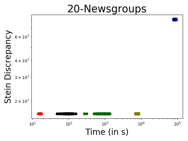
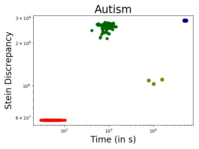
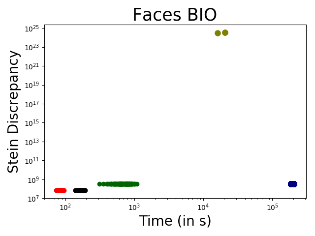
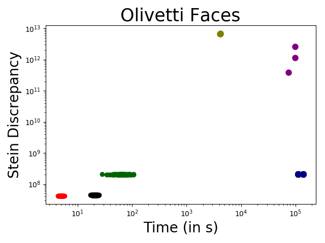
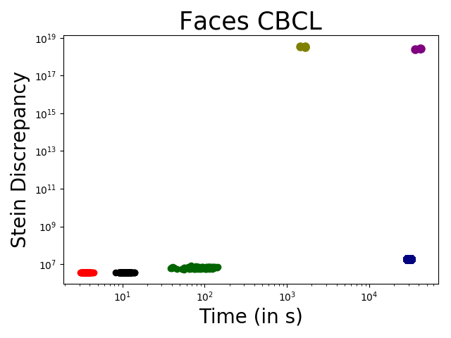
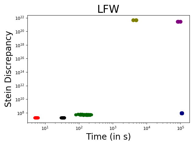
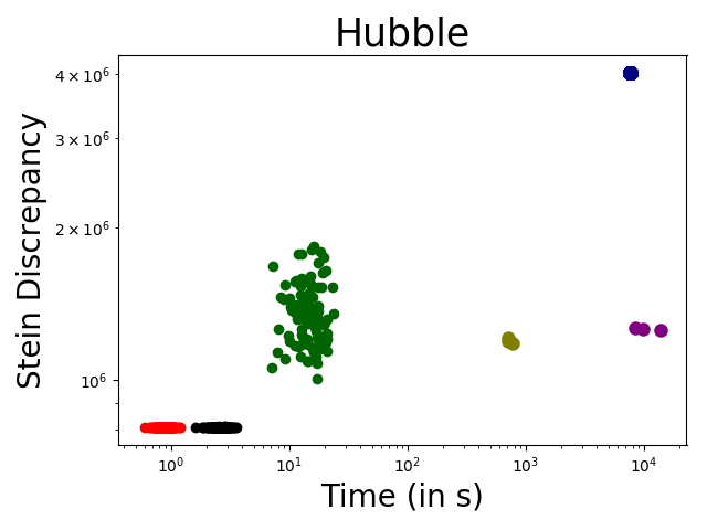
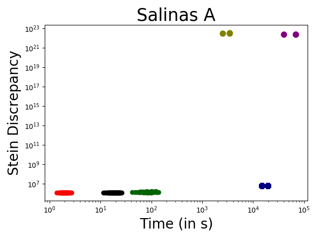
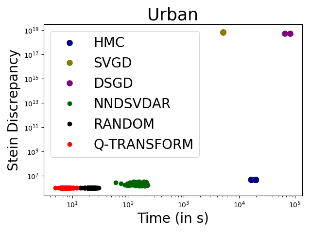
Figure 3: For each dataset we show the the quality of the Bayesian NMF approximate posterior ($M=5$) and the corresponding runtime of $Q$-Transform and the other baselines. Across multiple datasets, we see that the best discrete posteriors to Bayesian NMF (lowest Stein discrepancy) are produced in the least time using the Q-Transform initializations (in red).

The Stein discrepancy variational objective involves terms that consider both the quality of the factorizations (as given by the score function $\nabla_{\theta}\log p(\theta)$ ) and their similarity (as given by the base RKHS kernel $k(\theta_{i},\theta_{j})$). The initialization-based approaches ($Q$-Transform, Random and NNDSVD) are all designed to find high quality factorizations (as defined by the SILF Likelihood). The diversity of high-quality factorizations therefore plays an important role in determining the Stein discrepancy. In figure 3, we see that both $Q$-Transform and the approach that substitutes $Q$-Transform initializations for random restarts (labelled Random), obtain the highest quality posterior approximations for $M=5$ and the $Q$-Transform approach consistently takes less time. The NNDSVDar initializations and thinned HMC samples lead to factorizations that are high-quality but often not diverse (see diversity analysis in supplementary material: figures 15, 16, 17). The SVGD and the DSGD are generally the worst performing algorithms. These methods are often unable to find factorization parameters that meet the quality criteria of the SILF likelihood (see quality analysis in supplementary material: figures 13 and 14). This is understandable because even using simple gradient-based approaches to find a single high-quality NMF turns out to be difficult, hence the existence of a literature on specialized algorithms for performing NMF.

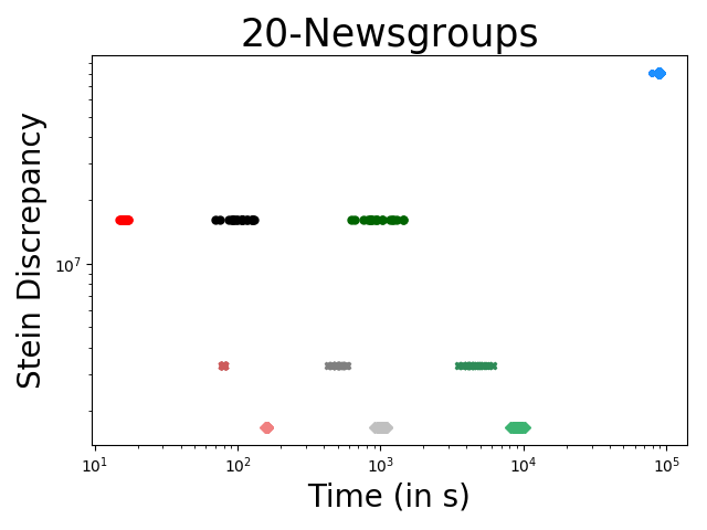
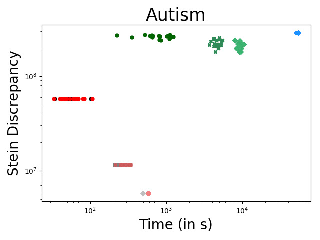
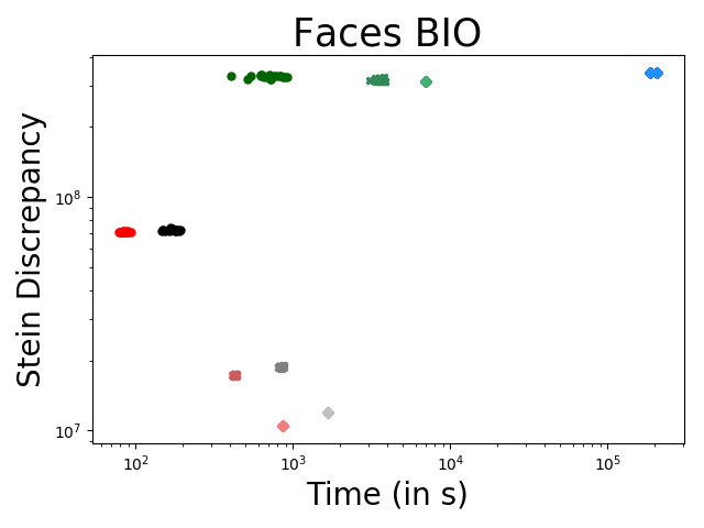
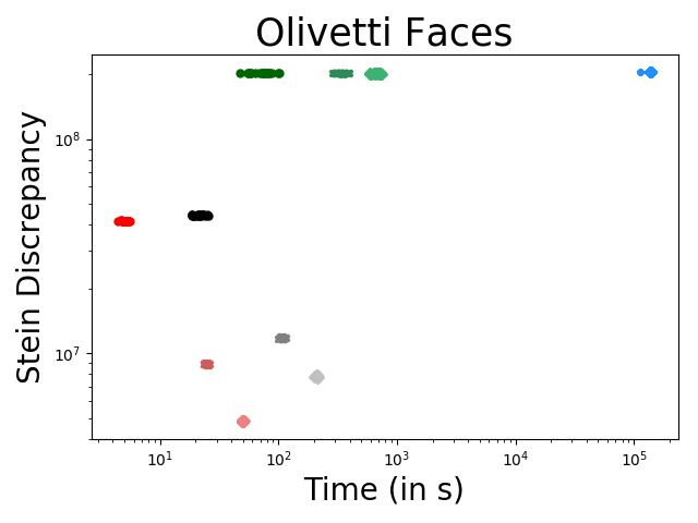
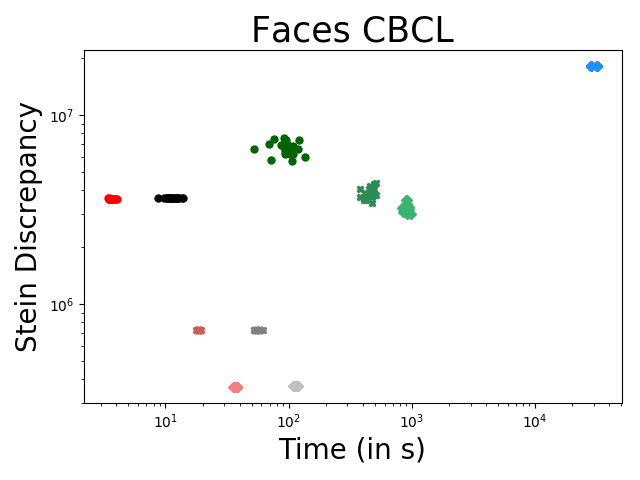
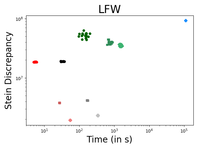
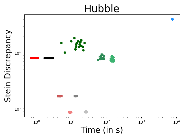
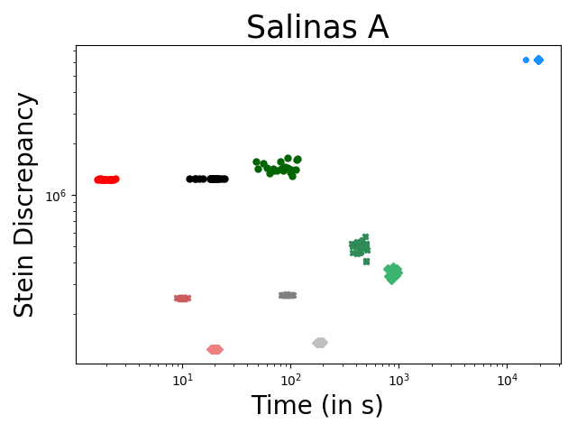
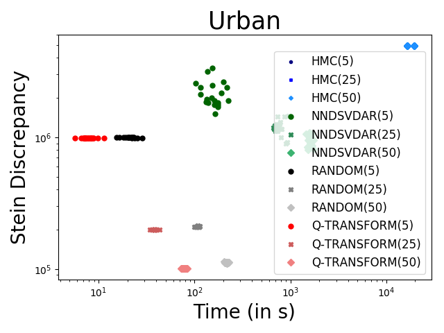
Figure 4: For each dataset we show the the quality of the Bayesian NMF approximate posterior (for $M=\{5,25,50\}$) and the corresponding runtime of $Q$-Transform and the other baselines (except SVGD and SDGD). Across multiple datasets, we see that the best discrete posteriors to Bayesian NMF (lowest Stein discrepancy) are produced in the least time using the Q-Transform initializations (in red).

Figure 4 shows results for $M=\{5,25,50\}$ where $Q$-Transform continues to have a runtime advantage over other baselines. Additionally, for some datasets (Olivetti Faces, LFW and Faces BIO) $Q$-Transform also produces higher quality of the posterior approximations. Variational posteriors constructed using thinned samples from HMC significantly lack diversity as the Stein discrepancies for collections of size 5, 25 and 50 are comparable. This indicates that the HMC chain only explores a small region of the posterior distribution and can be confirmed through the diversity analysis in the supplementary material (figures 15, 16, 17). Sminchisescu et al. (2007) notes that in high dimensional spaces, we expect there to be many ridges of probability as there are likely to be some directions in which the posterior density decays sharply. Alternatively, there may be several isolated modes with no connecting regions of high probability making it particularly challenging for the HMC chain to avoid getting stuck in a local mode of the Bayesian NMF posterior.

7.2 Interpretation and Utilization of Posterior Estimates

NMF posteriors can provide insight into the non-identifiability present within a particular dataset. Different factorizations may explain the data as a whole equally well, but do it through dictionary elements that have different interpretations or can be used to understand specific parts of the data better than other factorizations. We show visual examples of diversity in the top words of the 20 Newsgroups NMF posteriors and examples of how performance in downstream tasks for the 20 Newsgroups and Autism dataset is dependent on the posterior samples. Our analysis yields meaningful insights that could not be gained through a single factorization.

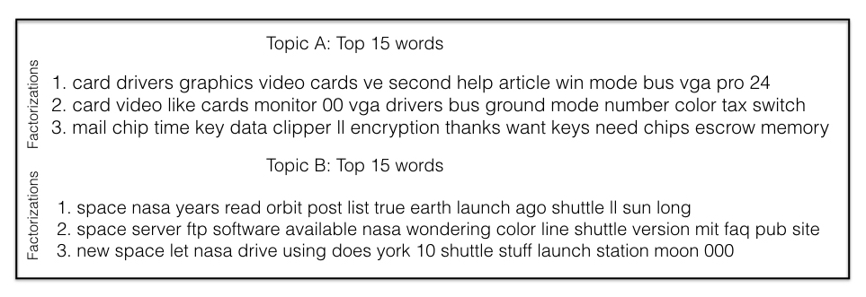
Figure 5: The top 15 words for topic A (computers/electronics) and topic B (space) shows that different factorizations provide an emphasis on different terms. In topic A, the top word from factorization 1 and 2 is ‘card’, but it does not appear in the top 15 words of factorizations 3. Instead a similar term ‘chip’ is emphasized in Factorization 3. In topic B, the terms ‘space’ and ‘nasa’ appear in all three factorizations but factorization 2 is the only one with digital terms like ‘ftp’, ’server’,’site’ and ’faq’. In contrast factorization 1 and 3 both contain more physical terms like ‘sun’, ‘moon’,‘launch’.

20-Newsgroups

Our Bayesian NMF of 20-Newsgroups in section 7.1 was a rank 16 decomposition of posts from 4 categories. In figure 6, we show the held-out AUC of a classifier trained to predict those categories based on the weight matrix $W$ from each factorization in our variational posterior. Even though all of these factorizations have essentially equivalent reconstruction (see figure 14 in supplementary material), there exists a significant variation in the performance of these NMFs on the prediction tasks. The best performing NMF for one category is generally not the best (or even one of the top performing) NMFs for other categories. This observation may be valuable to a practitioner intending to use the NMF for some downstream task: different samples explain different patterns in the data. In figure 5, we see that this is indeed true: even after alignment, distinct NMF factorizations have top words that indicate different emphasis across topics.

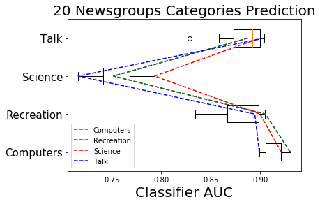
Figure 6: Classifiers trained on feature vectors from different factorizations yield variability in prediction performance (as measured by AUC). The dotted lines show the factorization that produces the best performing classifier for each category. The factorization (blue dotted line) that predicts the ‘Talk’ category best is actually one of the worst performing factorizations for the ‘Science’ category. This variability in performance demonstrates that no single factorization gives the best latent representation for the overall prediction task.

Autism Spectrum Disorder (ASD)

In addition to core autism symptoms, Doshi-Velez et al. (2014) describe three major subtypes in autism spectrum disorder: those with higher rates of neurological disorder, those with higher rates of autoimmune disorders, and those with higher rates of psychiatric disorders. In figure 7, we show the number of topics that contain key terms corresponding to these areas (expressive language disorder, epilepsy, asthma, and attention deficit disorder) across different factorizations in the variational posterior obtained via $Q$-Transform. The large variation suggests that different factorizations in the particle-based posterior are spending different amount of modeling effort across these known factors; knowing that such uncertainty exists is essential for clinicians who may be trying to interpret topics to understand patterns in autism spectrum disorder.

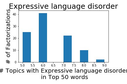
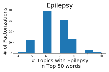
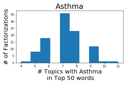
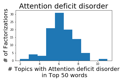
Figure 7: We explore top words in the topics relating to key terms of interest to clinicians and discover that different NMFs place varying amount of emphasis on different terms. Such variability is of interest to clinicians who may be trying to interpret topics to understand patterns in ASD.

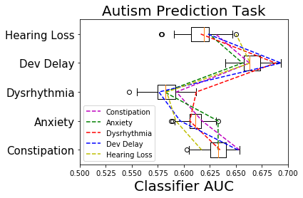
Figure 8: Classifiers trained on weights matrix of $M_{\text{max}}=100$ different factorizations to predict the presence of certain medical codes in a patient’s trajectory exhibit significant variability in prediction on a test set (as measured by AUC). Different factorizations lead to top predictors for the onset of different medical issues.

On the same set of patients, we can also ask whether we can predict the onset of certain medical issues in the subsequent patient trajectory. We train a classifier on the weights of the NMFs to predict the onset of these medical issues. Similar to the category prediction results in 20-Newsgroups, figure  8 shows that there is a large variability (around 0.1 in AUC) in the performance of classifiers trained on the weights matrices of different factorizations on the prediction task. No single factorization has the best performance across the different prediction tasks.

7.3 Extension: Bayesian NMF in the presence of missing data

In the presence of missing data, there is perhaps an even greater need to understand the uncertainty in factorization parameters for NMF. The factorization space of a fully observed dataset forms a subset of the factorization space in the presence of missing data. Our particle-based approach to Bayesian NMF posterior approximation can be applied to the missing data setting by making some minor adjustments to the experimental settings.

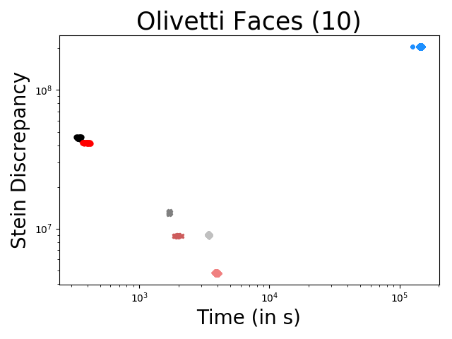
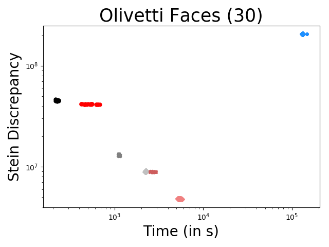
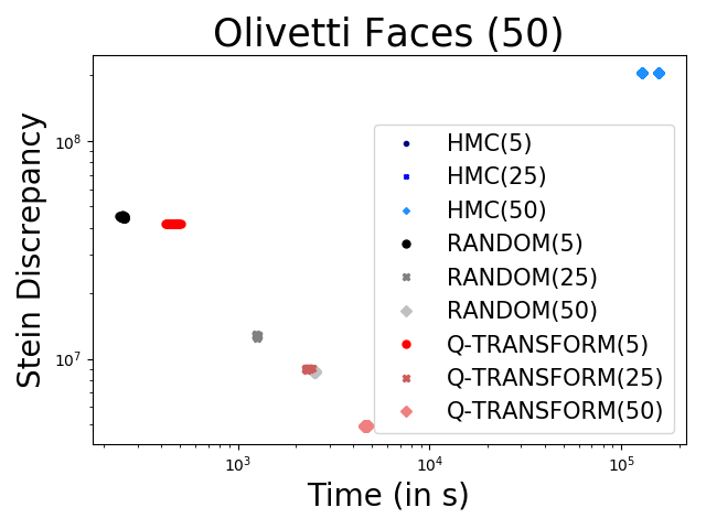
Figure 9: Under different percentages of missing-ness in the Olivetti Faces dataset (10%, 30%, 50%), the quality of the Bayesian NMF approximate posterior and the corresponding runtime of $Q$-Transform and the other baselines is shown. The best discrete posterior approximations to Bayesian NMF are produced using the Q-Transform initializations (in red).

The multiplicative update algorithm for NMF (Lee and Seung, 2001) can be adjusted so that the update equations for factorization parameters only consider the observed data. We use an implementation of this modification to the multiplicative update algorithm to find a completion of the data $X$, compute the SVD subspace and then apply our $Q$-Transform initializations. Figure 9 demonstrates that our approach to Bayesian NMF can be extended to the case where the data matrix $X$ is partially observed. For the Olivetti Faces dataset with varying degrees of missing-ness, the $Q$-Transform approach to Bayesian NMF consistently finds posterior approximations that are significantly better (as measured by Stein Discrepancy) than other baselines whereas for a given $M$, the runtime is second-lowest.

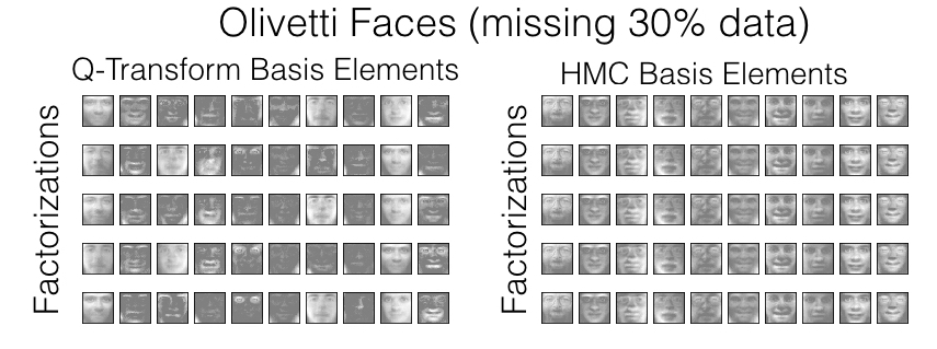
Figure 10: Sample factorizations from the variational posterior using $Q$-Transforms show that a diverse range of basis elements can be use to approximate the data. However, HMC samples seem to be identical indicating that HMC was only exploring a very small region of the posterior space.

Figure 10 shows sample factorizations from the variational posterior using $Q$-Transform and HMC samples. To allow for comparison, we have aligned the positions of the basis (dictionary) elements to a reference factorization using the bipartite matching algorithm. It is clear from looking at the $Q$-Transform factorizations that a diverse range of dictionaries can be used to approximate the data well whereas the HMC chain only explores one set of dictionary elements. Interestingly, the diversity of solutions obtained using $Q$-Transform have visually interpretable differences, i.e. these are not simply perturbations of some ground truth basis elements. Some of the basis elements look like faces and some of them look like different shadow or lighting configurations. In contrast, the factorization samples from HMC have basis elements that look identical. This indicates that the HMC has explored a limited region of the posterior space.

8 Discussion: When is $Q$-Transform successful?

Our ability to extract transferrable low-rank transformation matrices from an SVD and an instance of NMF indicates that there exist some shared similarities between the SVD and NMFs. In this section we seek to develop a better intuition behind the success of the $Q$-Transform initializations at exploiting these similarities. We investigate the effect of noise on the quality of the initializations and the resulting time-advantage in optimization. In addition, we explore the choice of transfer rank $R_{T}$ and its effect on the quality of initializations. Lastly, we describe a practical implementation consideration regarding consistency of convention used in the SVD.

8.1 The $Q$-Transform Initialization versus Noise

In Section 4, we sought high-quality initializations because they generally require less time to converge. On synthetic data $X=AW+\epsilon N_{o}$ (D = N = 500, K = 20) we explore the effect of increasing noise ($\epsilon$) on the quality of our transfer-based NMF initializations and the time taken to converge. We normalize the norm of the noise matrix to be equal to the norm of the data $\|N_{o}\|=\|AW\|$ so that the contribution of signal $AW$ and noise $\epsilon N_{o}$ to the data is equal when $\epsilon=1$. We continue to use the same $100$ pairs of $Q_{A},Q_{W}$ matrices. We compare the performance of $Q$-Transform over random restarts in terms of initialization quality (ratio of the reconstruction error from $Q$-Transform to the reconstruction error from random restart) and time to convergence (ratio of time taken using $Q$-Transform initialization to time taken using random restart). In both metrics, the $Q$-Transform has an advantage over random restarts for values of the noise $\epsilon$ smaller than $1$, and the advantage is greatest for smallest noise. Figure 11 shows that the advantage of $Q$-Transform initializations is highest in a low noise regime and decreases as the noise increases. This behavior makes sense because as noise increases, the data is no longer truly low rank.

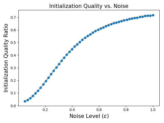
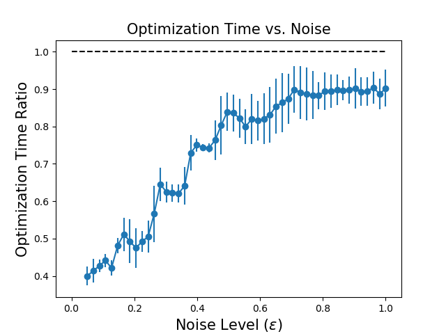
Figure 11: In the low-noise regime, the reconstruction error of $Q$-Transform initializations is significantly less than random restart initializations. This relative advantage gets smaller as the noise level increases. Similarly, the time taken to converge is significantly shorter than the random restart approach under the low noise scenario and continues to increase with noise. As expected, at high noise levels there exists no additional advantage to the $Q$-Transform approach (the optimization time ratio approaches 1).

8.2 Selecting transformation dimensions $R_{T}$ and $R_{\text{SVD}}$:

Transformation matrices $Q_{A},Q_{W}$ map basis vectors defining the top SVD subspace of dimension $R_{\text{SVD}}$ to a set of $R_{T}$ non-negative basis vectors that approximate the same subspace. The full initialization for NMF is obtained by either padding the initialization with small entries ($R_{T}<R_{\text{NMF}}$) or removing extra columns and rows of the factor matrices ($R_{T}>R_{\text{NMF}}$). For simplicity, we consider the case where the transfer rank and SVD rank are equal $R_{T}=R_{\text{SVD}}$ and the resulting transformation matrices $Q_{A},Q_{W}$ are square. In our experiments on real data, we chose the transfer rank and SVD rank $R_{T}=R_{\text{SVD}}=3$ and demonstrate that it successfully produces the highest quality approximate posteriors in the least amount of time. In practice, we could have chosen from a range of values to determine the transfer rank $R_{T}$ and SVD rank $R_{\text{SVD}}$.

To investigate, we extract a set of $100$ transformation matrices $Q_{A},Q_{W}$ for transfer dimensions $R_{T}=R_{\text{SVD}}=\{1,2,\ldots,10\}$ using synthetic data ($D=N=15$). Once constructed, we applied the transformation matrices to a $500\times 500$ dataset $X_{\text{TEST}}$ of rank $K=10$. Figure 12 shows the quality of the initialization from each of the different transfer dimensions explored. Even though the dataset $X_{\text{TEST}}$ has rank $10$, the rank $10$ transformation matrices found using the $15\times 15$ synthetic dataset are unable to successfully transfer to this new dataset. We see a general trend that as the transfer rank increases, the quality of the initializations gets worse. This tells us that the transformations of the top-most singular vectors of the data most consistently transfer to new datasets whereas the transformations of singular vectors corresponding to smaller singular values are less consistently transferred to new datasets.

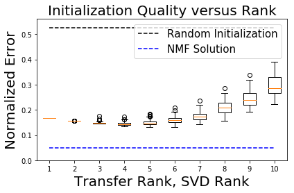
Figure 12: On a synthetic dataset ($D=N=500,K_{\text{NMF}}=10$), we apply $Q$-Transform initializations using varying transfer ranks and SVD ranks $R_{T}=R_{\text{SVD}}=\{1,2,\ldots,10\}$. We see that for a range of low rank values, the $Q$-Transform initializations are high quality, but at larger values the quality of initializations gets worse. The black dotted line shows the highest quality random initialization and the blue dotted line shows the lowest quality NMF solution. The reconstruction errors are normalized by the norm of the data.

8.3 Sign Convention for SVD

In considering when $Q$-Transform is successful, we note that there exists an intrinsic ambiguity in the sign of the singular vectors of $X$: changing the sign of any column of $A_{\text{SVD}}$ and corresponding row of $W_{\text{SVD}}$ gives a valid SVD. For $Q$-Transform to work, we must apply a consistent resolution of the sign ambiguity (e.g. from Bro et al. (2008)). This ensures that learned transformations $Q_{A},Q_{W}$ map in a consistent way to SVD decompositions of new datasets.

9 Related Work

Recent work on NMF has involved theoretical work on non-identifiability with new algorithms that can provably recover the NMF under certain assumptions (Li and Liang, 2017; Bhattacharya et al., 2016; Ge and Zou, 2015a). However, these assumptions are often difficult to check and may indeed be violated in practice.

There is a large body of work on Bayesian NMF. Sampling-based approaches include Gibbs sampling (Schmidt et al., 2009), Hamiltonian Monte Carlo (Schmidt and Mohamed, 2009), and reversible jump variants (Schmidt and Mørup, 2010). All of these have trouble escaping local modes (Masood et al., 2016), and are often constrained to a limited class of tractable distributions. Variational approaches to Bayesian NMF have successfully yielded interpretable factorizations (Bertin et al., 2009; Cemgil, 2009; Paisley et al., 2014) but also typically only capture one mode. We note that in many cases, priors of convenience—for example, exponential distributions—can induce a single dominant mode, even when that was not the intent of the practitioner. Gershman et al. (2012) develop a non-parametric approach to variational inference that provides flexibility in modeling the number of Gaussian components required to approximate a posterior. However, the isotropic covariance in the model makes it unsuitable for applying it to Bayesian NMF.

The ability of Stein discrepancies to assess the quality of any collection of particles (Gorham and Mackey, 2015) has resulted in large recent interest in other ways to create collections of samples (Oates et al., 2017; Liu and Wang, 2016). Liu et al. (2016) and Chwialkowski et al. (2016) showed that kernelized Stein discrepancy could be computed analytically in Reproducing Kernel Hilbert Spaces (RKHS); Pu et al. (2017) and Wang et al. use neural networks instead. Ranganath et al. (2016) establish the Stein discrepancy as a valid variational objective. To our knowledge, Stein discrepancy-based posterior approximation has not been applied to NMF, and yet, we see that it allows us to leverage existing non-Bayesian approaches to characterize these multi-modal posteriors. In our work, the Dirichlet prior on the columns of the basis matrix $A$ is important to ensure that we avoid a known saddle point of the zero factorization (from likelihood term) that yields a corresponding zero for the score function.

Our $Q$-Transform approach to finding multiple optima is most similar to Ročková and George (2016) and Paatero and Tapper (1994),

who use rotations to find solutions to a single matrix factorization problem that are sparse and non-negative respectively. In contrast, we use rotations to find multiple non-negative solutions, and also demonstrate how these rotations can be re-used for transfer learning.

10 Conclusion

In this work, we presented a novel transfer learning-based approach to posterior estimation in Bayesian NMF. Simply creating collections of factorizations via random restarts or our $Q$-Transform initializations, and then weighing them, produces diverse collections that approximate the posterior well (the NNDSVDar-based methods fail to produce diverse collections for posterior estimation). In contrast, the functional gradient descent of SVGD and direct gradients of Stein discrepancy (DSGD) perform worse to the collection-based approaches, requiring more time and also limiting the user to specify in advance the number of factorizations. Hamiltonian Monte Carlo also suffers from difficulties in exploring the posterior space, something random initializations are well suited to. Our transfer learning approach consistently produces the highest quality posterior approximations.

Through $Q$-Transform, we introduce a way to speed-up the process of finding multiple diverse NMFs. The discovery that $Q$-Transform matrices can transfer from synthetic to multiple real datasets is exciting and also suggests interesting questions for further research. For example, what is the theoretical nature of the similarities between principal eigenspaces of different non-negative matrices and the relation between their SVD and NMF bases? And, how does the synthetic data generation process used to obtain $Q$-Transform matrices impact the initializations and the effectiveness of the $Q$-Transform algorithm in general?

More broadly, our qualitative results demonstrate that even relatively simple models, such as NMF, can have multiple optima that are comparable under the objective function but have large variation in how well they explain different portions of the data—or how they perform on different downstream tasks. Thus, it is important to be able to compute these posteriors efficiently.

Acknowledgments

We would like to thank Andreas Krause, Mike Hughes, Melanie Pradier, Nick Foti, Omer Gottesman and other members of the Dtak lab at Harvard for many helpful conversations and feedback. MAM and FDV acknowledge support from AFOSR FA 9550-17-1-0155.

Appendix A: Quality of factorizations

We measure the quality of factorizations in terms of the log of the joint likelihood (figure 13) as well the Frobenius NMF objective (figure 14). We see that both quality measures are in agreement with each other. $Q$-Transform, Random, NNDSVDar and HMC produce high quality factorizations. The initialization-based approaches all work well as they use specialized NMF algorithms that are designed to find high quality factorizations. HMC was given a warm start with a high likelihood initialization and the chain continues to stay in high likelihood regions. The remaining gradient-based approaches for optimizing a collection of particles (SVGD and DSGD) fail to produce high quality factorizations. This is indicative of the need for specialized NMF algorithms designed to work with the constraints and structure of the NMF problem and highlight how difficult it is to apply a naive gradient descent approach for finding NMFs. The objective function in DSGD is the Stein discrepancy, but $Q$-Transform (and almost all other baselines) perform better in that objective than DSGD.

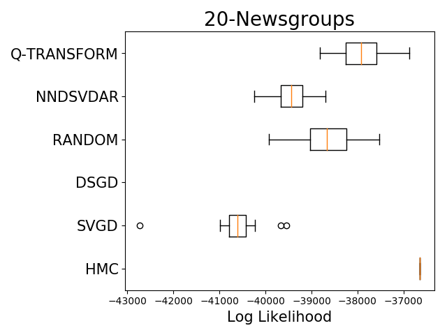
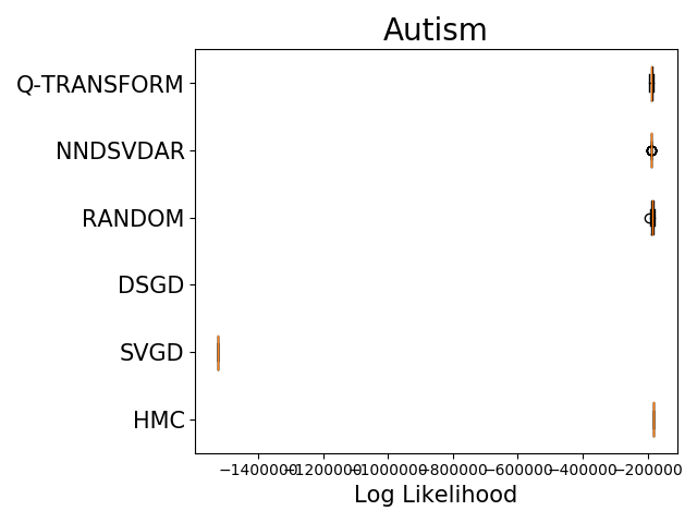
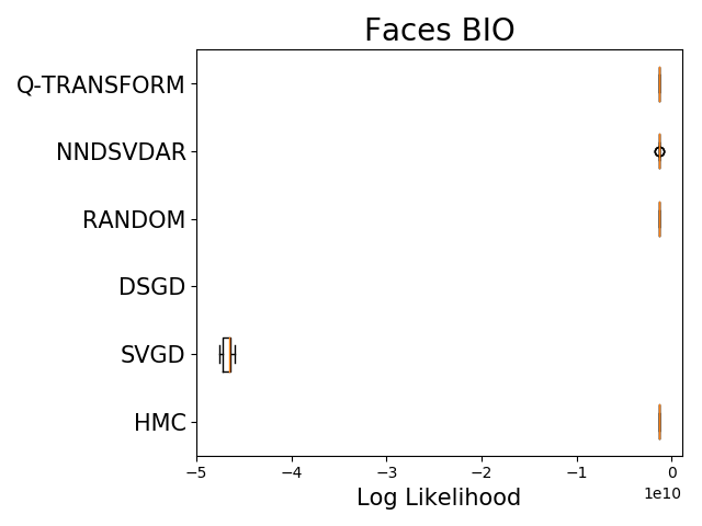
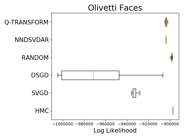
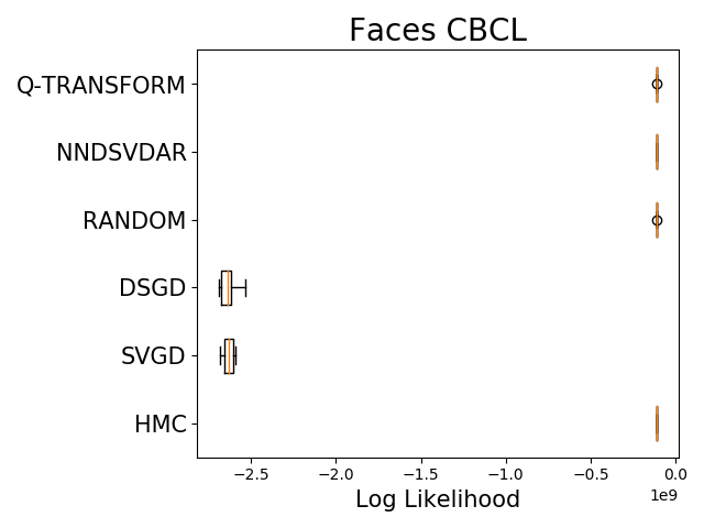
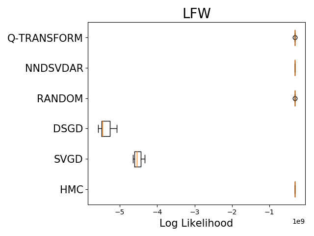
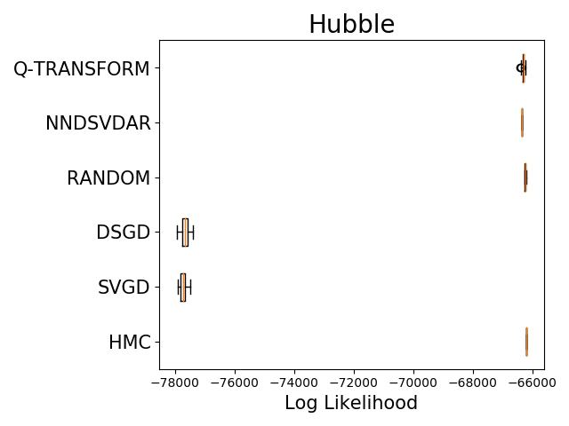
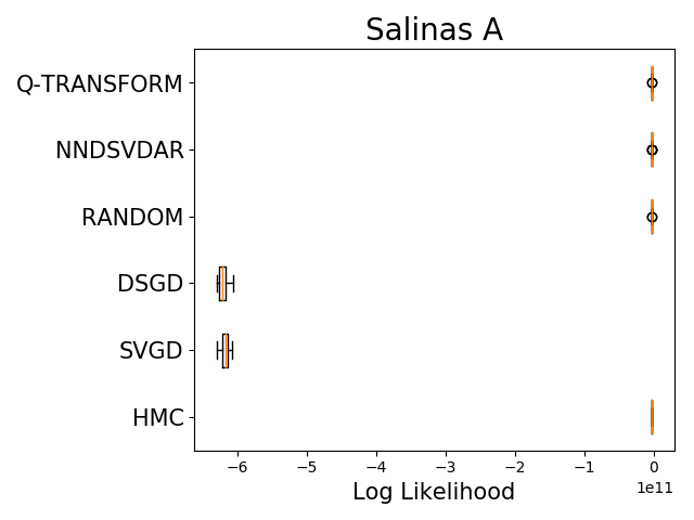
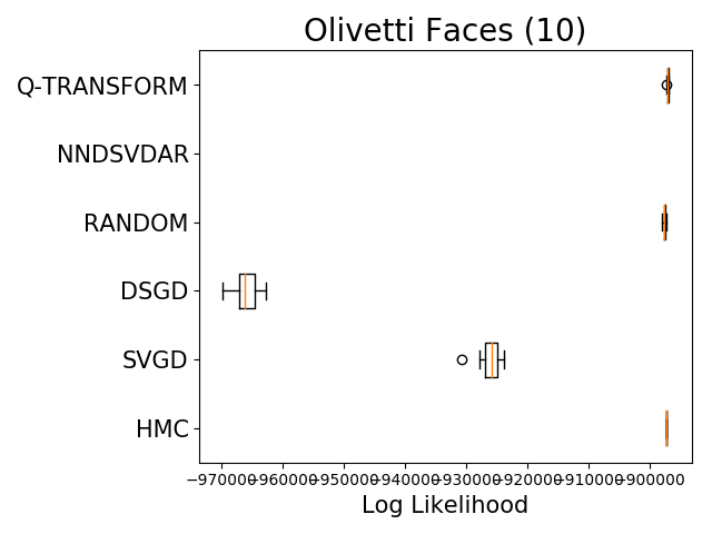
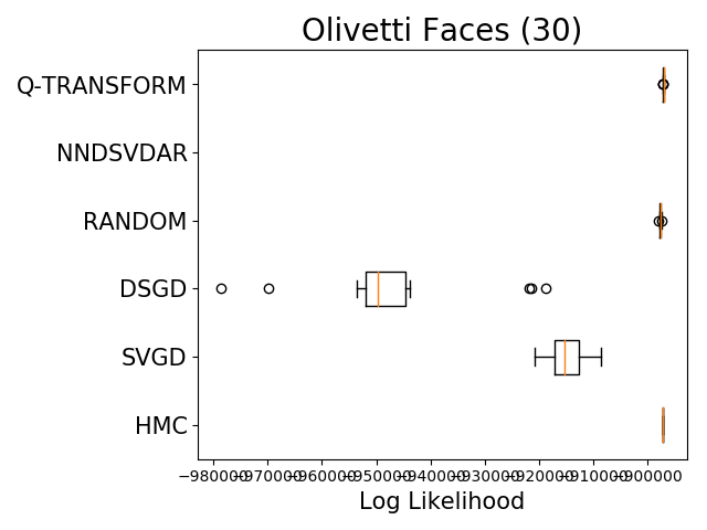
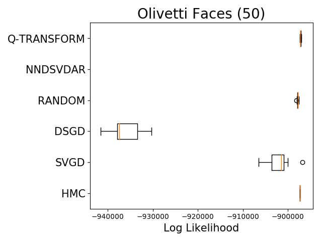
Figure 13: The joint likelihood of factorizations shows that SVGD and DSGD generally produce the worst quality factorizations. HMC, NNDSVDar, Random and $Q$-Transform produce high quality factorizations.

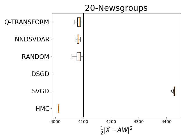
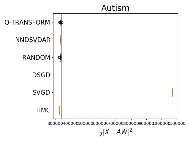
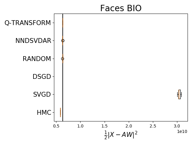
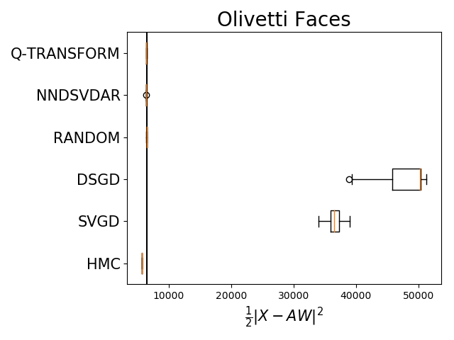
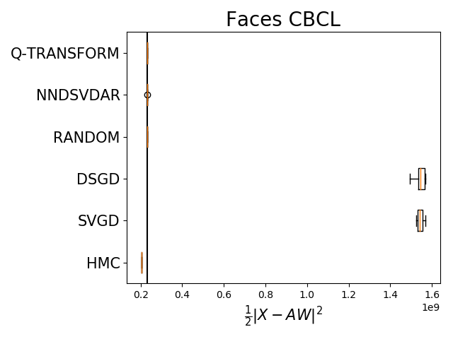
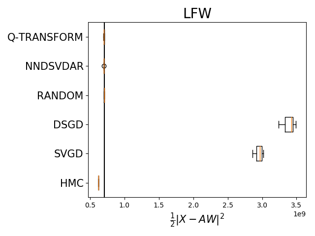
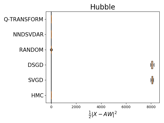
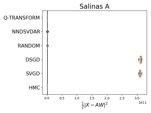
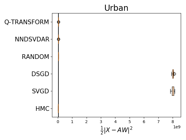
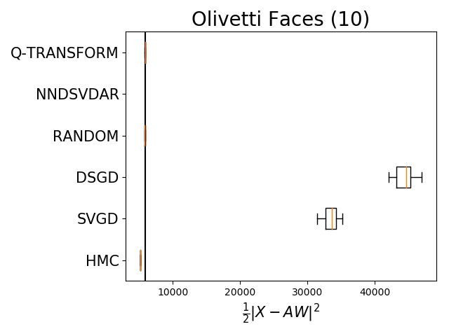
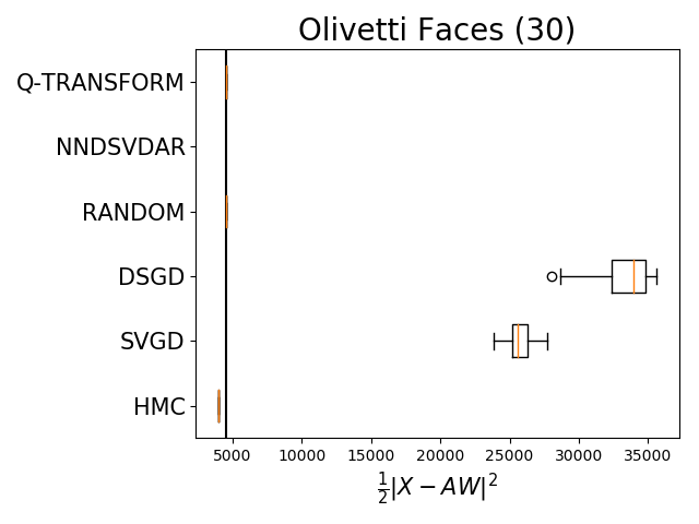
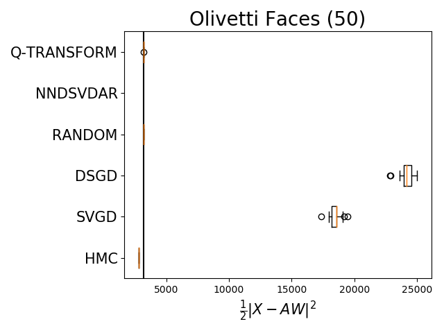
Figure 14: The reconstruction error of the factorizations shows that SVGD and DSGD are typically unable to find factorization parameters that meet the threshold quality (black line) for useful factorizations. The other approaches consistently produce factorizations that meet this minimum quality requirement.

Appendix B: Diversity of factorizations

We take a closer look at the diversity of factorizations produced by our $Q$-Transform and competing baseline approaches. Similarity of factorizations is measured by the kernel (equation 7) for the base RKHS (figure 15) used in evaluating the Stein discrepancy and by pairwise distances between basis matrices (figure 16) and weights matrices (figure 17). The different diversity metrics tell the same story. The HMC chain exhibits the least exploration of the factorization space followed by NNDSVDar. SVGD, DSGD, Random and $Q$-Transform all exhibit the higher amounts of exploration in the factorization space, but the exploration in SVGD and DSGD does not correspond to high likelihood regions of the posterior therefore it is unimportant.

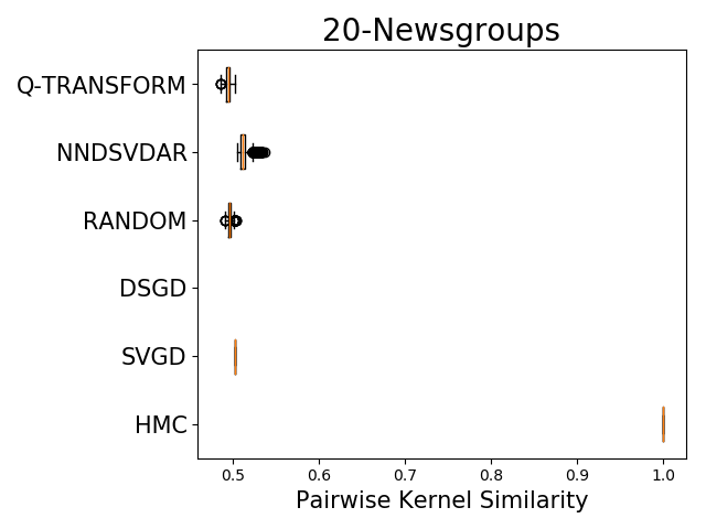
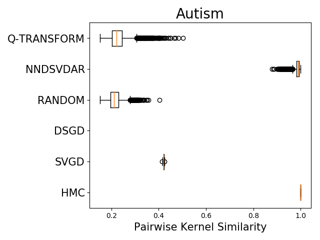
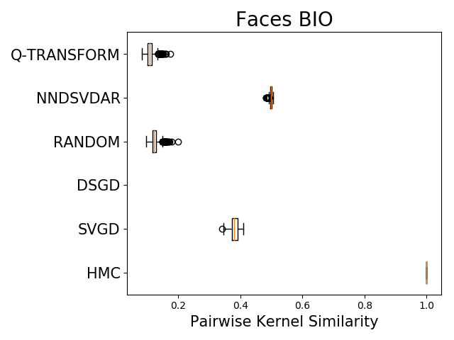
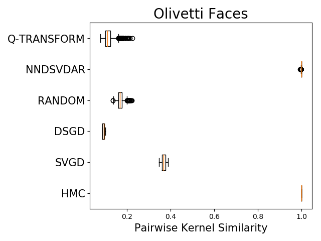
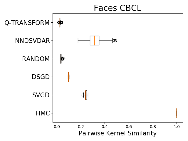
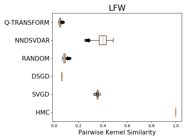
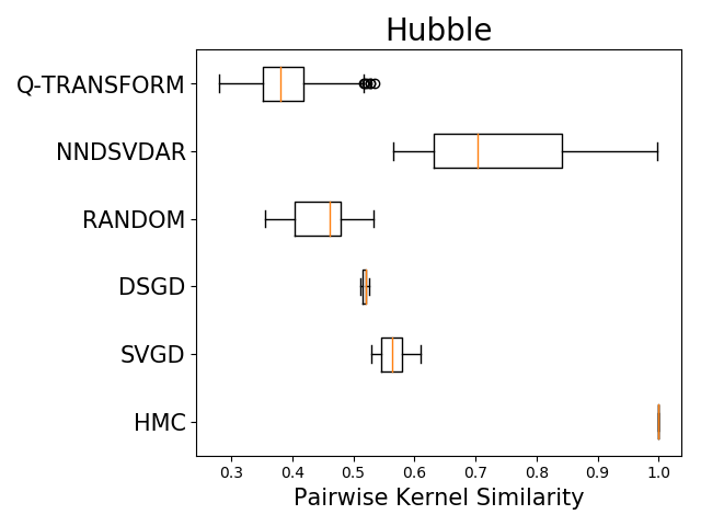
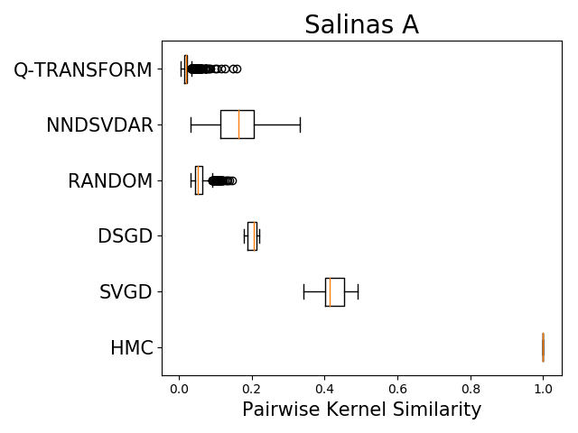
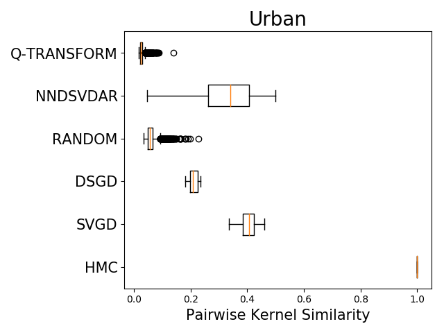
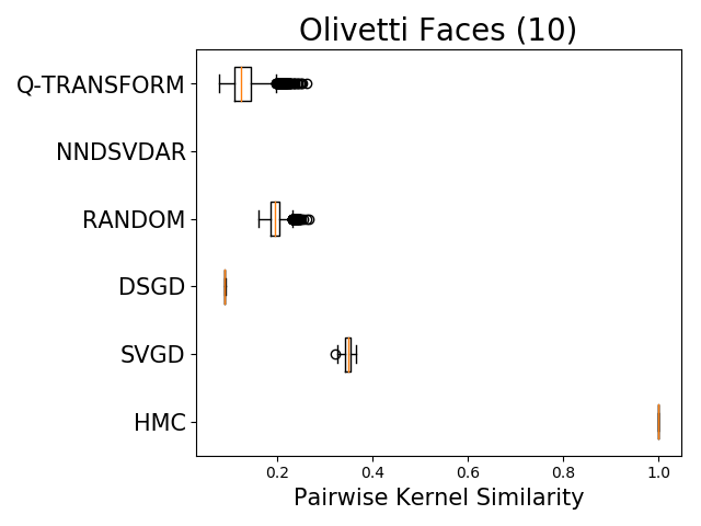
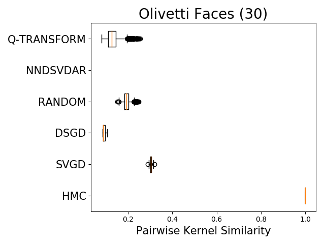
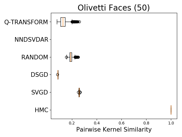
Figure 15: The kernel similarity indicates that factorization collections obtained by HMC are most similar indicating that the HMC chain is only exploring a small region of the posterior. In many cases NNDSVDar factorizations are also very similar. $Q$-Transform and Random are the only algorithms that produce factorizations of high quality that are not similar.

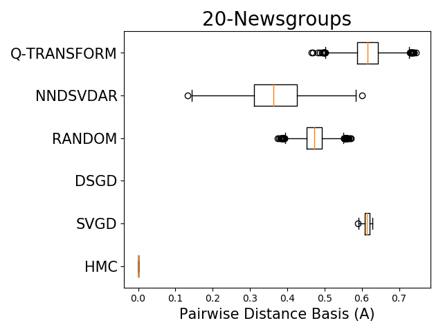
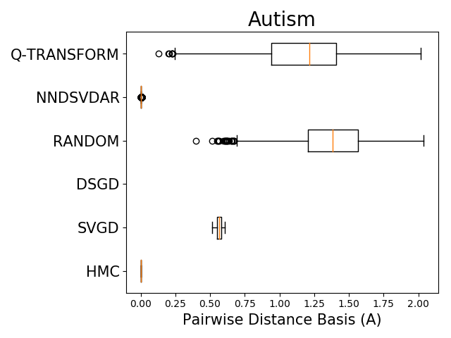
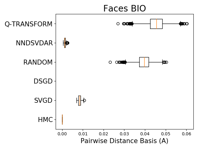
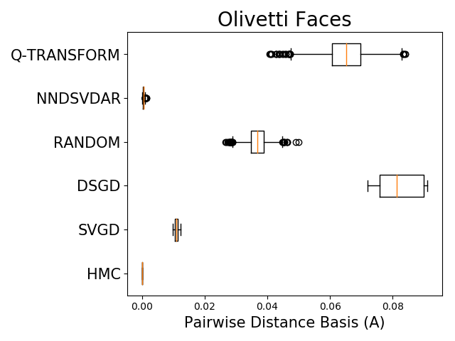
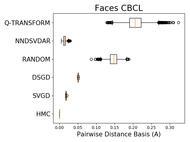
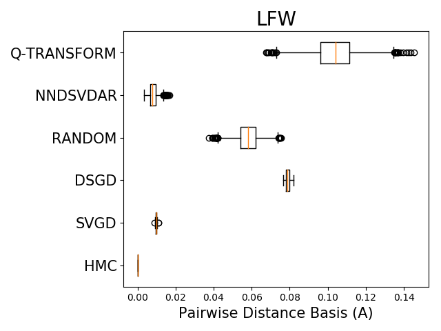
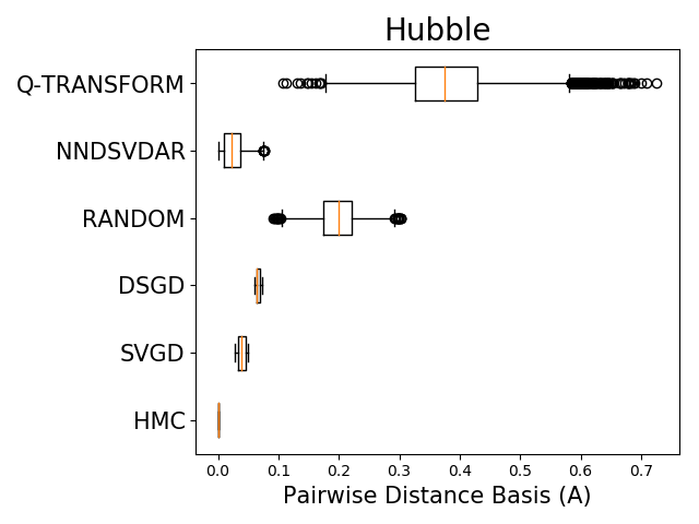
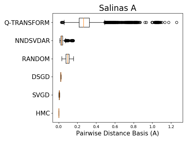
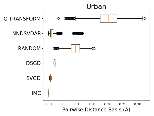
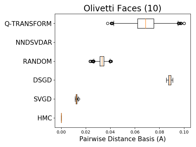
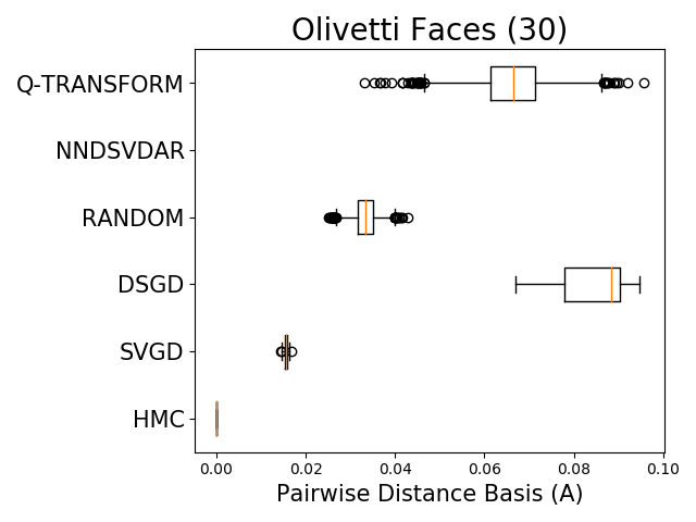
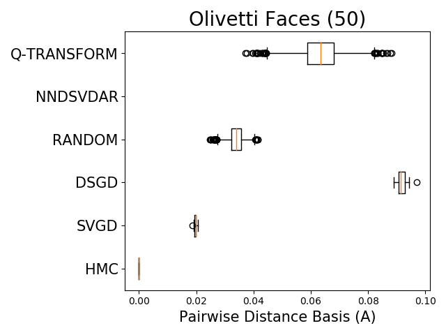
Figure 16: The pairwise distance between basis matrices shows that factorization collections obtained by HMC are most similar indicating that the HMC chain is only exploring a small region of the posterior. In many cases NNDSVDar factorizations are also very similar. $Q$-Transform and Random are the only algorithms that produce factorizations of high quality that are different.

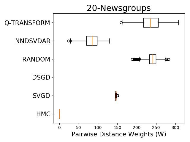
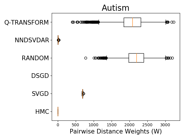
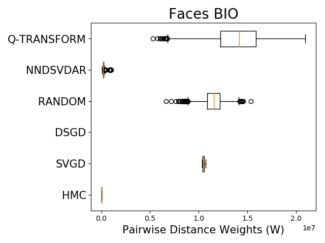
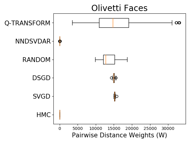
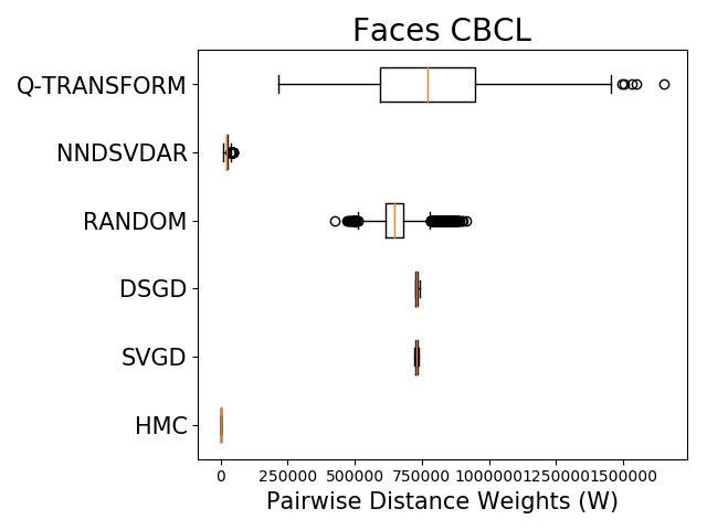
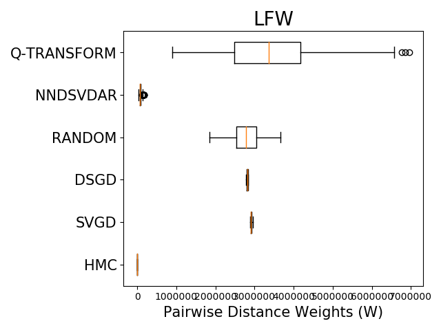
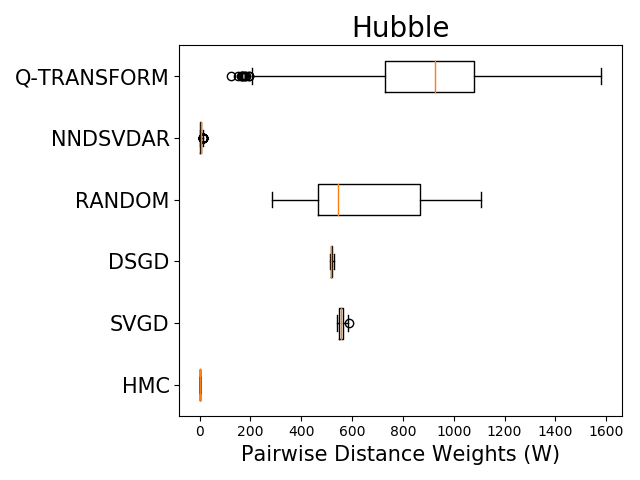
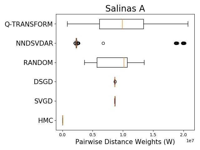
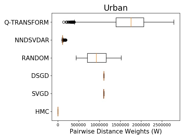
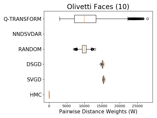
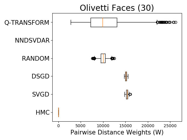
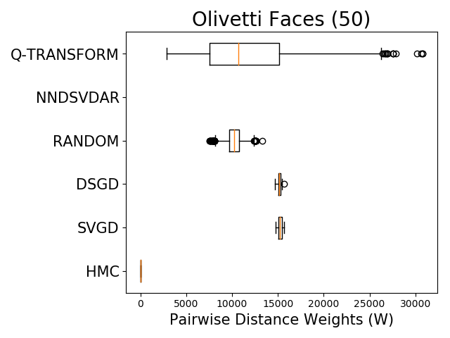
Figure 17: The pairwise distance between weights matrices shows that factorization collections obtained by HMC are most similar indicating that the HMC chain is only exploring a small region of the posterior. In many cases NNDSVDar factorizations are also very similar. $Q$-Transform and Random are the only algorithms that produce factorizations of high quality that are different.

References

- (1) 20NG. The 20 newsgroups text dataset ? scikit-learn 0.19.1 documentation. http://scikit-learn.org/stable/datasets/twenty_newsgroups.html. (Accessed on 01/23/2018).
- Altmann et al. (2014) Yoann Altmann, Nicolas Dobigeon, and Jean-Yves Tourneret. Unsupervised post-nonlinear unmixing of hyperspectral images using a hamiltonian monte carlo algorithm. IEEE Transactions on Image Processing, 23(6):2663–2675, 2014.
- Arngren et al. (2011) Morten Arngren, Mikkel N Schmidt, and Jan Larsen. Unmixing of hyperspectral images using bayesian non-negative matrix factorization with volume prior. Journal of Signal Processing Systems, 65(3):479–496, 2011.
- Arora et al. (2012) Sanjeev Arora, Rong Ge, Ravindran Kannan, and Ankur Moitra. Computing a nonnegative matrix factorization–provably. In Proceedings of the forty-fourth annual ACM symposium on Theory of computing, pages 145–162. ACM, 2012.
- Baydin et al. (2015) Atilim Gunes Baydin, Barak A Pearlmutter, Alexey Andreyevich Radul, and Jeffrey Mark Siskind. Automatic differentiation in machine learning: a survey. arXiv preprint arXiv:1502.05767, 2015.
- Bertin et al. (2009) Nancy Bertin, Roland Badeau, and Emmanuel Vincent. Fast bayesian nmf algorithms enforcing harmonicity and temporal continuity in polyphonic music transcription. In Applications of Signal Processing to Audio and Acoustics, 2009. WASPAA’09. IEEE Workshop on, pages 29–32. IEEE, 2009.
- Betancourt (2012) Michael Betancourt. Cruising the simplex: Hamiltonian monte carlo and the dirichlet distribution. In AIP Conference Proceedings 31st, volume 1443, pages 157–164. AIP, 2012.
- Bhattacharya et al. (2016) Chiranjib Bhattacharya, Navin Goyal, Ravindran Kannan, and Jagdeep Pani. Non-negative matrix factorization under heavy noise. In International Conference on Machine Learning, pages 1426–1434, 2016.
- Bhattacharyya et al. (2016) Chiranjib Bhattacharyya, IISC ERNET, Navin Goyal, COM Ravindran Kannan, and COM Jagdeep Pani. Non-negative matrix factorization under heavy noise. In Proceedings of The 33rd International Conference on Machine Learning, pages 1426–1434, 2016.
- (10) BIOFACES. Bioid face database — dataset for face detection — facedb. https://www.bioid.com/facedb/. (Accessed on 01/23/2018).
- Bioucas-Dias et al. (2012) José M Bioucas-Dias, Antonio Plaza, Nicolas Dobigeon, Mario Parente, Qian Du, Paul Gader, and Jocelyn Chanussot. Hyperspectral unmixing overview: Geometrical, statistical, and sparse regression-based approaches. Selected Topics in Applied Earth Observations and Remote Sensing, IEEE Journal of, 5(2):354–379, 2012.
- Boutsidis and Gallopoulos (2008) Christos Boutsidis and Efstratios Gallopoulos. Svd based initialization: A head start for nonnegative matrix factorization. Pattern Recognition, 41(4):1350–1362, 2008.
- Bro et al. (2008) Rasmus Bro, Evrim Acar, and Tamara G Kolda. Resolving the sign ambiguity in the singular value decomposition. Journal of Chemometrics, 22(2):135–140, 2008.
- Brunet et al. (2004) Jean-Philippe Brunet, Pablo Tamayo, Todd R Golub, and Jill P Mesirov. Metagenes and molecular pattern discovery using matrix factorization. PNAS, 101(12):4164–4169, 2004.
- (15) CBCL. Home — poggio lab. http://poggio-lab.mit.edu/. (Accessed on 01/23/2018).
- Cemgil (2009) Ali Taylan Cemgil. Bayesian inference for nonnegative matrix factorisation models. Computational Intelligence and Neuroscience, 2009, 2009.
- Chu et al. (2004) Wei Chu, S Sathiya Keerthi, and Chong Jin Ong. Bayesian support vector regression using a unified loss function. IEEE transactions on neural networks, 15(1):29–44, 2004.
- Chwialkowski et al. (2016) Kacper Chwialkowski, Heiko Strathmann, and Arthur Gretton. A kernel test of goodness of fit. arXiv preprint arXiv:1602.02964, 2016.
- Cichocki and Phan (2009) Andrzej Cichocki and Anh-Huy Phan. Fast local algorithms for large scale nonnegative matrix and tensor factorizations. IEICE transactions on fundamentals of electronics, communications and computer sciences, 92(3):708–721, 2009.
- Diamond and Boyd (2016) Steven Diamond and Stephen Boyd. Cvxpy: A python-embedded modeling language for convex optimization. The Journal of Machine Learning Research, 17(1):2909–2913, 2016.
- Dikmen and Cemgil (2009) Onur Dikmen and A Taylan Cemgil. Unsupervised single-channel source separation using bayesian nmf. In Applications of Signal Processing to Audio and Acoustics, 2009. WASPAA’09. IEEE Workshop on, pages 93–96. IEEE, 2009.
- Donoho and Stodden (2003) David Donoho and Victoria Stodden. When does non-negative matrix factorization give a correct decomposition into parts? In Advances in neural information processing systems, page None, 2003.
- Doshi-Velez et al. (2014) Finale Doshi-Velez, Yaorong Ge, and Isaac Kohane. Comorbidity clusters in autism spectrum disorders: an electronic health record time-series analysis. Pediatrics, 133(1):e54–e63, 2014.
- Févotte and Idier (2011) Cédric Févotte and Jérôme Idier. Algorithms for nonnegative matrix factorization with the -divergence. Neural computation, 23(9):2421–2456, 2011.
- Févotte et al. (2009) Cédric Févotte, Nancy Bertin, and Jean-Louis Durrieu. Nonnegative matrix factorization with the itakura-saito divergence: With application to music analysis. Neural computation, 21(3):793–830, 2009.
- Ge and Zou (2015a) Rong Ge and James Zou. Intersecting faces: Non-negative matrix factorization with new guarantees. In International Conference on Machine Learning, pages 2295–2303, 2015a.
- Ge and Zou (2015b) Rong Ge and James Zou. Intersecting faces: Non-negative matrix factorization with new guarantees. In International Conference on Machine Learning, page X. ICML, 2015b.
- Gendreau and Potvin (2010) Michel Gendreau and Jean-Yves Potvin. Handbook of metaheuristics, volume 2. Springer, 2010.
- Gershman et al. (2012) Samuel J Gershman, Matthew D Hoffman, and David M Blei. Nonparametric variational inference. 2012.
- Gorham and Mackey (2015) Jackson Gorham and Lester Mackey. Measuring sample quality with stein’s method. In Advances in Neural Information Processing Systems, pages 226–234, 2015.
- Gorham and Mackey (2017) Jackson Gorham and Lester Mackey. Measuring sample quality with kernels. arXiv preprint arXiv:1703.01717, 2017.
- Greene et al. (2008) Derek Greene, Gerard Cagney, Nevan Krogan, and Pádraig Cunningham. Ensemble non-negative matrix factorization methods for clustering protein–protein interactions. Bioinformatics, 2008.
- Gretton et al. (2006) Arthur Gretton, Karsten M Borgwardt, Malte Rasch, Bernhard Schölkopf, and Alex J Smola. A kernel method for the two-sample-problem. In Advances in neural information processing systems, pages 513–520, 2006.
- Halko et al. (2009) Nathan Halko, Per-Gunnar Martinsson, and Joel A Tropp. Finding structure with randomness: Stochastic algorithms for constructing approximate matrix decompositions. 2009.
- Hoffman and Blei (2015) Matthew D Hoffman and David M Blei. Structured stochastic variational inference. In Artificial Intelligence and Statistics, 2015.
- Hsieh and Dhillon (2011) Cho-Jui Hsieh and Inderjit S Dhillon. Fast coordinate descent methods with variable selection for non-negative matrix factorization. In Proceedings of the 17th ACM SIGKDD international conference on Knowledge discovery and data mining, pages 1064–1072. ACM, 2011.
- Laurberg et al. (2008) H. Laurberg, M. Christensen, M. Plumbley, L. Hansen, and S. Jensen. Theorems on positive data: on the uniqueness of nmf. Computational Intelligence and Neuroscience, 2008.
- Lee and Seung (2001) Daniel D Lee and H Sebastian Seung. Algorithms for non-negative matrix factorization. In Advances in neural information processing systems, pages 556–562, 2001.
- (39) LFW. Lfw face database : Main. http://vis-www.cs.umass.edu/lfw/. (Accessed on 01/23/2018).
- Li and Liang (2017) Yuanzhi Li and Yingyu Liang. Provable alternating gradient descent for non-negative matrix factorization with strong correlations. arXiv preprint arXiv:1706.04097, 2017.
- Lin (2007) Chih-Jen Lin. Projected gradient methods for nonnegative matrix factorization. Neural computation, 19(10):2756–2779, 2007.
- Liu and Feng (2016) Qiang Liu and Yihao Feng. Two methods for wild variational inference. arXiv preprint arXiv:1612.00081, 2016.
- Liu and Lee (2016) Qiang Liu and Jason D Lee. Black-box importance sampling. arXiv preprint arXiv:1610.05247, 2016.
- Liu and Wang (2016) Qiang Liu and Dilin Wang. Stein variational gradient descent: A general purpose bayesian inference algorithm. In Advances in Neural Information Processing Systems, pages 2370–2378, 2016.
- Liu et al. (2016) Qiang Liu, Jason Lee, and Michael Jordan. A kernelized stein discrepancy for goodness-of-fit tests. In International Conference on Machine Learning, pages 276–284, 2016.
- Maclaurin et al. (2015) Dougal Maclaurin, David Duvenaud, and Ryan P Adams. Autograd: Reverse-mode differentiation of native python. In ICML workshop on Automatic Machine Learning, 2015.
- Masood et al. (2016) Arjumand Masood, Weiwei Pan, and Finale Doshi-Velez. An empirical comparison of sampling quality metrics: A case study for bayesian nonnegative matrix factorization. arXiv preprint arXiv:1606.06250, 2016.
- Moussaoui et al. (2006) Saïd Moussaoui, David Brie, Ali Mohammad-Djafari, and Cédric Carteret. Separation of non-negative mixture of non-negative sources using a bayesian approach and mcmc sampling. Signal Processing, IEEE Transactions on, 54(11):4133–4145, 2006.
- Neal et al. (2011) Radford M Neal et al. Mcmc using hamiltonian dynamics. Handbook of Markov Chain Monte Carlo, 2:113–162, 2011.
- Nicolas Gillis (1987) Robert J. Plemmons Nicolas Gillis. Hubble telescope hyperspectral image data, 1987. URL https://sites.google.com/site/nicolasgillis/code.
- Oates et al. (2017) Chris J Oates, Mark Girolami, and Nicolas Chopin. Control functionals for monte carlo integration. Journal of the Royal Statistical Society: Series B (Statistical Methodology), 79(3):695–718, 2017.
- Olah et al. (2018) Chris Olah, Arvind Satyanarayan, Ian Johnson, Shan Carter, Ludwig Schubert, Katherine Ye, and Alexander Mordvintsev. The building blocks of interpretability. Distill, 2018. doi: 10.23915/distill.00010. https://distill.pub/2018/building-blocks.
- Paatero and Tapper (1994) Pentti Paatero and Unto Tapper. Positive matrix factorization: A non-negative factor model with optimal utilization of error estimates of data values. Environmetrics, 5(2):111–126, 1994.
- Paisley et al. (2015) John Paisley, David M Blei, and Michael I Jordan. Bayesian nonnegative matrix factorization with stochastic variational inference. Handbook of Mixed Membership Models and Their Applications. Chapman and Hall/CRC, 2015.
- Paisley et al. (2014) John William Paisley, David M Blei, and Michael I Jordan. Bayesian nonnegative matrix factorization with stochastic variational inference., 2014.
- Pan and Yang (2010) Sinno Jialin Pan and Qiang Yang. A survey on transfer learning. IEEE Transactions on knowledge and data engineering, 22(10):1345–1359, 2010.
- Pan and Doshi-Velez (2016) Weiwei Pan and Finale Doshi-Velez. A characterization of the non-uniqueness of nonnegative matrix factorizations. arXiv preprint arXiv:1604.00653, 2016.
- Patterson and Teh (2013) Sam Patterson and Yee Whye Teh. Stochastic gradient riemannian langevin dynamics on the probability simplex. In Advances in Neural Information Processing Systems, pages 3102–3110, 2013.
- Pedregosa et al. (2011) Fabian Pedregosa, Gaël Varoquaux, Alexandre Gramfort, Vincent Michel, Bertrand Thirion, Olivier Grisel, Mathieu Blondel, Peter Prettenhofer, Ron Weiss, Vincent Dubourg, et al. Scikit-learn: Machine learning in python. Journal of Machine Learning Research, 12(Oct):2825–2830, 2011.
- Pu et al. (2017) Yunchen Pu, Zhe Gan, Ricardo Henao, Chunyuan Li, Shaobo Han, and Lawrence Carin. Stein variational autoencoder. arXiv preprint arXiv:1704.05155, 2017.
- Ranganath et al. (2016) Rajesh Ranganath, Dustin Tran, Jaan Altosaar, and David Blei. Operator variational inference. In Advances in Neural Information Processing Systems, pages 496–504, 2016.
- Roberts et al. (2016) Margaret E Roberts, Brandon M Stewart, and Dustin Tingley. Navigating the local modes of big data. Computational Social Science, page 51, 2016.
- Ročková and George (2016) Veronika Ročková and Edward I George. Fast bayesian factor analysis via automatic rotations to sparsity. Journal of the American Statistical Association, 111(516):1608–1622, 2016.
- Salakhutdinov et al. (2002) Ruslan Salakhutdinov, Sam Roweis, and Zoubin Ghahramani. On the convergence of bound optimization algorithms. In Proceedings of the Nineteenth conference on Uncertainty in Artificial Intelligence, pages 509–516. Morgan Kaufmann Publishers Inc., 2002.
- (65) SalinasA. Multispec — home. https://engineering.purdue.edu/~biehl/MultiSpec/. (Accessed on 01/23/2018).
- Samaria (1994) Ferdinando S. Samaria. The database of faces (olivetti), 1994. URL http://www.cl.cam.ac.uk/research/dtg/attarchive/facedatabase.html.
- Schmidt and Mohamed (2009) Mikkel N Schmidt and Shakir Mohamed. Probabilistic non-negative tensor factorization using markov chain monte carlo. In Signal Processing Conference, 2009 17th European, pages 1918–1922. IEEE, 2009.
- Schmidt and Mørup (2010) Mikkel N Schmidt and Morten Mørup. Reversible jump mcmc for bayesian nmf. In Proc. NIPS Workshop on Monte Carlo Methods for Modern Applications, 2010.
- Schmidt et al. (2009) Mikkel N Schmidt, Ole Winther, and Lars Kai Hansen. Bayesian non-negative matrix factorization. In Independent Component Analysis and Signal Separation, pages 540–547. Springer, 2009.
- Smaragdis and Brown (2003) Paris Smaragdis and Judith C Brown. Non-negative matrix factorization for polyphonic music transcription. In Applications of Signal Processing to Audio and Acoustics, 2003 IEEE Workshop on., pages 177–180. IEEE, 2003.
- Sminchisescu et al. (2007) Cristian Sminchisescu, Max Welling, and G Hinton. Generalized darting monte carlo. In AISTATS, pages 516–523. Citeseer, 2007.
- Vavasis (2009) Stephen A Vavasis. On the complexity of nonnegative matrix factorization. SIAM Journal on Optimization, 20(3):1364–1377, 2009.
- (73) Dilin Wang, Yihao Feng, and Qiang Liu. Learning to sample using stein discrepancy.
- Wild et al. (2004) Stefan Wild, James Curry, and Anne Dougherty. Improving non-negative matrix factorizations through structured initialization. Pattern recognition, 37(11):2217–2232, 2004.
- Xue et al. (2008) Yun Xue, Chong Sze Tong, Ying Chen, and Wen-Sheng Chen. Clustering-based initialization for non-negative matrix factorization. Applied Mathematics and Computation, 205(2):525–536, 2008.
- Zhu et al. (2014) Feiyun Zhu, Ying Wang, Shiming Xiang, Bin Fan, and Chunhong Pan. Structured sparse method for hyperspectral unmixing. ISPRS Journal of Photogrammetry and Remote Sensing, 88:101–118, 2014.