Fast approximation and exact computation of negative curvature parameters of graphs^∗

Abstract.

In this paper, we study Gromov hyperbolicity and related parameters, that represent how close (locally) a metric space is to a tree from a metric point of view. The study of Gromov hyperbolicity for geodesic metric spaces can be reduced to the study of graph hyperbolicity. The main contribution of this paper is a new characterization of the hyperbolicity of graphs, via a new parameter which we call rooted insize. This characterization has algorithmic implications in the field of large-scale network analysis. A sharp estimate of graph hyperbolicity is useful, e.g., in embedding an undirected graph into hyperbolic space with minimum distortion [Verbeek and Suri, SoCG’14]. The hyperbolicity of a graph can be computed in polynomial-time, however it is unlikely that it can be done in subcubic time. This makes this parameter difficult to compute or to approximate on large graphs. Using our new characterization of graph hyperbolicity, we provide a simple factor 8 approximation algorithm (with an additive constant 1) for computing the hyperbolicity of an $n$-vertex graph $G=(V,E)$ in optimal time $O(n^{2})$ (assuming that the input is the distance matrix of the graph). This algorithm leads to constant factor approximations of other graph-parameters related to hyperbolicity (thinness, slimness, and insize). We also present the first efficient algorithms for exact computation of these parameters. All of our algorithms can be used to approximate the hyperbolicity of a geodesic metric space.

We also show that a similar characterization of hyperbolicity holds for all geodesic metric spaces endowed with a geodesic spanning tree. Along the way, we prove that any complete geodesic metric space $(X,d)$ has such a geodesic spanning tree.

1. Introduction

Understanding the geometric properties of complex networks is a key issue in network analysis and geometric graph theory. One important such property is negative curvature [27], causing the traffic between the vertices to pass through a relatively small core of the network – as if the shortest paths between them were curved inwards. It has been empirically observed, then formally proved [12], that such a phenomenon is related to the value of the Gromov hyperbolicity of the graph. In this paper, we propose exact and approximation algorithms to compute hyperbolicity of a graph and its relatives (the approximation algorithms can be applied to geodesic metric spaces as well).

A metric space $(X,d)$ is $\delta$-hyperbolic [3, 7, 24] if for any four points $w,v,x,y$ of $X$, the two largest of the distance sums $d(w,v)+d(x,y)$, $d(w,x)+d(v,y)$, $d(w,y)+d(v,x)$ differ by at most $2\delta\geq 0$. A graph $G=(V,E)$ endowed with its standard graph-distance $d_{G}$ is $\delta$-hyperbolic if the metric space $(V,d_{G})$ is $\delta$-hyperbolic. In case of geodesic metric spaces and graphs, $\delta$-hyperbolicity can be defined in other equivalent ways, e.g., via the thinness, slimness, or insize of geodesic triangles. The hyperbolicity $\delta(X)$ of a metric space $X$ is the smallest $\delta\geq 0$ such that $X$ is $\delta$-hyperbolic. It can be viewed as a local measure of how close $X$ is to a tree: the smaller the hyperbolicity is, the closer the metrics of its $4$-point subspaces are close to tree-metrics.

The study of hyperbolicity of graphs is motivated by the fact that many real-world graphs are tree-like from a metric point of view [1, 2, 4] or have small hyperbolicity [26, 27, 31]. This is due to the fact that many of these graphs (including Internet application networks, web networks, collaboration networks, social networks, biological networks, and others) possess certain geometric and topological characteristics. Hence, for many applications, including the design of efficient algorithms (cf., e.g., [4, 9, 10, 11, 12, 13, 17, 20, 33]), it is useful to know an accurate approximation of the hyperbolicity $\delta(G)$ of a graph $G$.

Related work.

For an $n$-vertex graph $G$, the definition of hyperbolicity directly implies a simple brute-force $O(n^{4})$ algorithm to compute $\delta(G)$. This running time is too slow for computing the hyperbolicity of large graphs that occur in applications [1, 4, 5, 22]. On the theoretical side, it was shown that relying on matrix multiplication results, one can improve the upper bound on time-complexity to $O(n^{3.69})$ [22]. Moreover, roughly quadratic lower bounds are known [5, 15, 22]. In practice, however, the best known algorithm still has an $O(n^{4})$-time worst-case bound but uses several clever tricks when compared to the brute-force algorithm [4]. Based on empirical studies, an $O(mn)$ running time is claimed, where $m$ is the number of edges in the graph. Furthermore, there are heuristics for computing the hyperbolicity of a given graph [14], and there are investigations of whether one can compute hyperbolicity in linear time when some graph parameters take small values [21, 16].

Perhaps it is interesting to notice that the first algorithms for computing the Gromov hyperbolicity were designed for Cayley graphs of finitely generated groups (these are infinite vertex-transitive graphs of uniformly bounded degrees). Gromov gave an algorithm to recognize Cayley graphs of hyperbolic groups and estimate the hyperbolicity constant $\delta$. His algorithm is based on the theorem that in Cayley graphs, the hyperbolicity “propagates”, i.e., if balls of an appropriate fixed radius induce a $\delta$-hyperbolic space, then the whole space is $\delta^{\prime}$-hyperbolic for some $\delta^{\prime}>\delta$ (see [24], 6.6.F and [18]). Therefore, in order to compute the hyperbolicity of a Cayley graph, it is enough to verify the hyperbolicity of a sufficiently big ball (all balls of a given radius in a Cayley graph are isomorphic to each other). For other algorithms deciding if the Cayley graph of a finitely generated group is hyperbolic, see [6, 29]. However, similar methods do not help when dealing with arbitrary graphs.

By a result of Gromov [24], if the four-point condition in the definition of hyperbolicity holds for a fixed basepoint $w$ and any triplet $x,y,v$ of $X$, then the metric space $(X,d)$ is $2\delta$-hyperbolic. This provides a factor 2 approximation of hyperbolicity of a metric space on $n$ points running in cubic $O(n^{3})$ time. Using fast algorithms for computing (max,min)-matrix products, it was noticed in [22] that this 2-approximation of hyperbolicity can be implemented in $O(n^{2.69})$ time. In the same paper, it was shown that any algorithm computing the hyperbolicity for a fixed basepoint in time $O(n^{2.05})$ would provide an algorithm for $(\max,\min)$-matrix multiplication faster than the existing ones. In [19], approximation algorithms are given to compute a $(1+\epsilon)$-approximation in $O(\epsilon^{-1}n^{3.38})$ time and a $(2+\epsilon)$-approximation in $O(\epsilon^{-1}n^{2.38})$ time. As a direct application of the characterization of hyperbolicity of graphs via a cop and robber game and dismantlability, [9] presents a simple constant factor approximation algorithm for hyperbolicity of $G$ running in optimal $O(n^{2})$ time. Its approximation ratio is huge (1569), however it is believed that its theoretical performance is much better and the factor of 1569 is mainly due to the use in the proof of the definition of hyperbolicity via linear isoperimetric inequality. This shows that the question of designing fast and (theoretically certified) accurate algorithms for approximating graph hyperbolicity is still an important and open question.

Our contribution.

In this paper, we tackle this open question and propose a very simple (and thus practical) factor 8 algorithm for approximating the hyperbolicity $\delta(G)$ of an $n$-vertex graph $G$ running in optimal $O(n^{2})$ time. As in several previous algorithms, we assume that the input is the distance matrix $D$ of the graph $G$. Our algorithm picks a basepoint $w$, a Breadth-First-Search tree $T$ rooted at $w$, and considers only geodesic triangles of $G$ with one vertex at $w$ and two sides on $T$. For all such sides in $T$, it computes the maximum over all distances between the two preimages of the centers of the respective tripods (see Section 2 for definitions). This maximum $\rho_{w,T}(G)$ (called rooted insize) can be easily computed in $O(n^{2})$ time and, as we demonstrate, provides an 8-approximation (with an additive constant 1) for $\delta(G)$. If the graph $G$ is given by its adjacency list, then we show that $\rho_{w,T}(G)$ can be computed in $O(nm)$ time and linear $O(n+m)$ space. For geodesic spaces $(X,d)$ endowed with a geodesic spanning tree we show that we can also define the rooted insize $\rho_{w,T}(X)$ and that the same relationships between $\rho_{w,T}(X)$ and the hyperbolicity $\delta(X)$ hold, thus providing a new characterization of hyperbolicity. En passant, we show that any complete geodesic space $(X,d)$ always has such a geodesic spanning tree (this result is not trivial, see the proof of Theorem 4.1 and Remark 4.4). We hope that this fundamental result can be useful in other contexts.

Perhaps it is surprising that hyperbolicity that is originally defined via quadruplets and can be 2-approximated via triplets (i.e., via pointed hyperbolicity), can be finally defined and approximated only via pairs (and an arbitrary fixed BFS-tree). Indeed, summarizing our contributions, we proved the existence of some property $P_{w,T}(x,y:\delta)$, defined w.r.t. a fixed basepoint $w$ and a fixed BFS tree $T$, such that: (i) for any $\delta$-hyperbolic graph the property holds for any pair $x,y$ of vertices; and conversely (ii) if the property holds for every pair $x,y$ then the graph is $8\delta$-hyperbolic. See Theorem 5.2 for more details. We hope that this new characterization can be useful in establishing that graphs and simplicial complexes occurring in geometry and in network analysis are hyperbolic.

The way the rooted insize $\rho_{w,T}(G)$ is computed is closely related to how hyperbolicity is defined via slimness, thinness, and insize of its geodesic triangles. Similarly to the hyperbolicity $\delta(G)$, one can define slimness $\varsigma(G)$, thinness $\tau(G)$, and insize $\iota(G)$ of a graph $G$. As a direct consequence of our algorithm for approximating $\delta(G)$ and the relationships between $\delta(G)$ and $\varsigma(G),\tau(G),\iota(G)$, we obtain constant factor $O(n^{2})$ time algorithms for approximating these parameters. On the other hand, an exact computation, in polynomial time, of these geometric parameters has never been provided. In Theorem 6.1, we show that the thinness $\tau(G)$ and the insize $\iota(G)$ of a graph $G$ can be computed in $O(n^{2}m)$ time and the slimness $\varsigma(G)$ of $G$ can be computed in $\widehat{O}(n^{2}m+n^{4}/\log^{3}n)$ time combinatorially and in $O(n^{3.273})$ time using matrix multiplication. However, we show that the minimum value of $\rho_{w,T}(G)$ over all basepoints $w$ and all BFS-trees $T$ cannot be approximated in polynomial time with a factor strictly better than 2 unless P = NP.

The new notion of rooted insize, as well as the classical notions of thinness, slimness, and insize can be defined only for unweighted graphs and geodesic metric spaces. Therefore, the approximation of hyperbolicity via the rooted insize (and the corresponding algorithms) do not hold for arbitrary metric spaces (such as weighted graphs for example).

2. Gromov hyperbolicity and its relatives

2.1. Gromov hyperbolicity

Let $(X,d)$ be a metric space and $w\in X$. The Gromov product of $y,z\in X$ with respect to $w$ is $(y|z)_{w}=\frac{1}{2}(d(y,w)+d(z,w)-d(y,z)).$ A metric space $(X,d)$ is $\delta$-hyperbolic [24] for $\delta\geq 0$ if $(x|y)_{w}\geq\min\{(x|z)_{w},(y|z)_{w}\}-\delta$ for all $w,x,y,z\in X$. Equivalently, $(X,d)$ is $\delta$-hyperbolic if for any $u,v,x,y\in X$, the two largest of the sums $d(u,v)+d(x,y)$, $d(u,x)+d(v,y)$, $d(u,y)+d(v,x)$ differ by at most $2\delta\geq 0$. A metric space $(X,d)$ is said to be $\delta$-hyperbolic with respect to a basepoint $w$ if $(x|y)_{w}\geq\min\{(x|z)_{w},(y|z)_{w}\}-\delta$ for all $x,y,z\in X$.

Proposition 2.1.

[3, 7, 24, 23] If $(X,d)$ is $\delta$-hyperbolic with respect to some basepoint, then $(X,d)$ is $2\delta$-hyperbolic.

Let $(X,d)$ be a metric space. An $(x,y)$-geodesic is a (continuous) map $\gamma:[0,d(x,y)]\to X$ from the segment $[0,d(x,y)]$ of ${\mathbb{R}}^{1}$ to $X$ such that $\gamma(0)=x,\gamma(d(x,y))=y,$ and $d(\gamma(s),\gamma(t))=|s-t|$ for all $s,t\in[0,d(x,y)].$ A geodesic segment with endpoints $x$ and $y$ is the image of the map $\gamma$ (when it is clear from the context, by a geodesic we mean a geodesic segment and we denote it by $[x,y]$). A metric space $(X,d)$ is geodesic if every pair of points in $X$ can be joined by a geodesic. A real tree (or an ${\mathbb{R}}$-tree) [7, p.186] is a geodesic metric space $(T,d)$ such that

1. there is a unique geodesic $[x,y]$ joining each pair of points $x,y\in T$;

2. if $[y,x]\cap[x,z]=\{x\}$, then $[y,x]\cup[x,z]=[y,z].$

Let $(X,d)$ be a geodesic metric space. A geodesic triangle $\Delta(x,y,z)$ with $x,y,z\in X$ is the union $[x,y]\cup[x,z]\cup[y,z]$ of three geodesics connecting these points. A geodesic triangle $\Delta(x,y,z)$ is called $\delta$-slim if for any point $u$ on the side $[x,y]$ the distance from $u$ to $[x,z]\cup[z,y]$ is at most $\delta$. Let $m_{x}$ be the point of $[y,z]$ located at distance $\alpha_{y}:=(x|z)_{y}$ from $y.$ Then, $m_{x}$ is located at distance $\alpha_{z}:=(y|x)_{z}$ from $z$ because $\alpha_{y}+\alpha_{z}=d(y,z)$. Analogously, define the points $m_{y}\in[x,z]$ and $m_{z}\in[x,y]$ both located at distance $\alpha_{x}:=(y|z)_{x}$ from $x;$ see Fig. 1 for an illustration. We define a tripod $T(x,y,z)$ consisting of three solid segments $[x,m],[y,m],$ and $[z,m]$ of lengths $\alpha_{x},\alpha_{y},$ and $\alpha_{z},$ respectively. The function mapping the vertices $x,y,z$ of $\Delta(x,y,z)$ to the respective leaves of $T(x,y,z)$ extends uniquely to a function $\varphi:\Delta(x,y,z)\to T(x,y,z)$ such that the restriction of $\varphi$ on each side of $\Delta(x,y,z)$ is an isometry. This function maps the points $m_{x},m_{y},$ and $m_{z}$ to the center $m$ of $T(x,y,z)$. Any other point of $T(x,y,z)$ is the image of at most two points of $\Delta(x,y,z)$. A geodesic triangle $\Delta(x,y,z)$ is called $\delta$-thin if for all points $u,v\in\Delta(x,y,z),$ $\varphi(u)=\varphi(v)$ implies $d(u,v)\leq\delta.$ The insize of $\Delta(x,y,z)$ is the diameter of the preimage $\{m_{x},m_{y},m_{z}\}$ of the center $m$ of the tripod $T(x,y,z)$. Below, we remind that the hyperbolicity of a geodesic space can be approximated by the maximum thinness and slimness of its geodesic triangles.

Figure 1. Insize and thinness in geodesic spaces and graphs.

For a geodesic metric space $(X,d)$, one can define the following parameters:

• hyperbolicity $\delta(X)=\min\{\delta:X\text{ is }\delta\text{-hyperbolic}\},$

• pointed hyperbolicity $\delta_{w}(X)=\min\{\delta:X\text{ is }\delta\text{-hyperbolic with respect to a basepoint }w\},$

• slimness $\varsigma(X)=\min\{\delta:\text{any geodesic triangle of }X\text{ is }\delta\text{-slim}\},$

• thinness $\tau(X)=\min\{\delta:\text{any geodesic triangle of }X\text{ is }\delta\text{-thin}\},$

• insize $\iota(X)=\min\{\delta:\text{the insize of any geodesic triangle of }X\text{ is at most }\delta\}.$

Proposition 2.2.

[3, 7, 24, 23, 32] For a geodesic metric space $(X,d)$, $\delta(X)\leq\iota(X)=\tau(X)\leq 4\delta(X)$, $\varsigma(X)\leq\tau(X)\leq 4\varsigma(X)$, and $\delta(X)\leq 2\varsigma(X)\leq 6\delta(X)$.

Due to Propositions 2.1 and 2.2, a geodesic metric space $(X,d)$ is called hyperbolic if one of the numbers $\delta(X),\delta_{w}(X),\varsigma(X),\tau(X),\iota(X)$ (and thus all) is finite. Notice also that a geodesic metric space $(X,d)$ is 0-hyperbolic if and only if $(X,d)$ is a real tree [7, p.399] (and in this case, $\varsigma(X)=\tau(X)=\iota(X)=\delta(X)=0$).

2.2. Hyperbolicity of graphs

All graphs $G=(V,E)$ occurring in this paper are undirected and connected, but not necessarily finite (in algorithmic results they will be supposed to be finite). For a vertex $v\in V$, we denote by $N_{G}(v)$ the open neighborhood of $v$, by $N_{G}[v]$ the closed neighborhood of $v$, and by $\deg_{G}(v)$ the degree of $v$ (when $G$ is clear from the context, the subscripts will be omitted). For any two vertices $x,y\in V,$ the distance $d(x,y)$ is the minimum number of edges in a path between $x$ and $y.$ Let $[x,y]$ denote a shortest path connecting vertices $x$ and $y$ in $G$; we call $[x,y]$ a geodesic between $x$ and $y$. The interval $I(u,v)=\{x\in V:d(u,x)+d(x,v)=d(u,v)\}$ consists of all vertices on $(u,v)$-geodesics. There is a strong analogy between the metric properties of graphs and geodesic metric spaces, due to their uniform local structure. Any graph $G=(V,E)$ gives rise to a geodesic space $(X_{G},d)$ (into which $G$ isometrically embeds) obtained by replacing each edge $xy$ of $G$ by a segment isometric to $[0,1]$ with ends at $x$ and $y$. $X_{G}$ is called a metric graph. Conversely, by [7, Proposition 8.45], any geodesic metric space $(X,d)$ is (3,1)-quasi-isometric to a graph $G=(V,E)$. This graph $G$ is constructed in the following way: let $V$ be an open maximal $\frac{1}{3}$-packing of $X$, i.e., $d(x,y)>\frac{1}{3}$ for any $x,y\in V$ (that exists by Zorn’s lemma). Then two points $x,y\in V$ are adjacent in $G$ if and only if $d(x,y)\leq 1$. Since hyperbolicity is preserved (up to a constant factor) by quasi-isometries, this reduces the computation of hyperbolicity for geodesic spaces to the case of graphs.

The notions of geodesic triangles, insize, $\delta$-slim and $\delta$-thin triangles can also be defined in case of graphs with the single difference that for graphs, the center of the tripod is not necessarily the image of any vertex on the sides of $\Delta(x,y,z).$ For graphs, we “discretize” the notion of $\delta$-thin triangles in the following way. We say that a geodesic triangle $\Delta(x,y,z)$ of a graph $G$ is $\delta$-thin if for any $v\in\{x,y,z\}$ and vertices $a\in[v,u]$ and $b\in[v,w]$ ($u,w\in\{x,y,z\}$, and $u,v,w$ are distinct), $d(v,a)=d(v,b)\leq(u|w)_{v}$ implies $d(a,b)\leq\delta$. A graph $G$ is $\delta$-thin, if all geodesic triangles in $G$ are $\delta$-thin. Given a geodesic triangle $\Delta(x,y,z):=[x,y]\cup[x,z]\cup[y,z]$ in $G$, let $x_{y}$ and $y_{x}$ be the vertices of $[z,x]$ and $[z,y]$, respectively, both at distance $\lfloor(x|y)_{z}\rfloor$ from $z$. Similarly, one can define vertices $x_{z},z_{x}$ and vertices $y_{z},z_{y};$ see Fig. 1. The insize of $\Delta(x,y,z)$ is defined as $\max\{d(y_{z},z_{y}),d(x_{y},y_{x}),d(x_{z},z_{x})\}$. An interval $I(x,y)$ is said to be $\kappa$-thin if $d(a,b)\leq\kappa$ for all $a,b\in I(x,y)$ with $d(x,a)=d(x,b).$ The smallest $\kappa$ for which all intervals of $G$ are $\kappa$-thin is called the interval thinness of $G$ and denoted by $\kappa(G)$. Denote also by $\delta(G)$, $\delta_{w}(G)$, $\varsigma(G)$, $\tau(G)$, and $\iota(G)$ respectively the hyperbolicity, the pointed hyperbolicity with respect to a basepoint $w$, the slimness, the thinness, and the insize of a graph $G$.

3. Auxiliary results

We will need the following inequalities between $\varsigma(G)$, $\tau(G)$, $\iota(G)$, and $\delta(G)$. They are known to be true for all geodesic spaces (see [3, 7, 24, 23, 32]). We present graph-theoretic proofs in case of graphs for completeness (and due to slight modifications in their definitions for graphs).

Proposition 3.1.

$\delta(G)-\frac{1}{2}\leq\iota(G)=\tau(G)\leq 4\delta(G)$, $\varsigma(G)\leq\tau(G)\leq 4\varsigma(G)$, $\delta(G)-\frac{1}{2}\leq 2\varsigma(G)\leq 6\delta(G)+1$, and $\kappa(G)\leq\min\{\tau(G),2\delta(G),2\varsigma(G)\}$.

The fact that $\delta(G)\leq 2\varsigma(G)+\frac{1}{2}$ is a result of Soto [32, Proposition II.20]. For our convenience, we reformulate and prove the other results in four lemmas, plus one auxiliary lemma.

Lemma 3.2.

$\varsigma(G)\leq\iota(G)=\tau(G)\leq 4\varsigma(G)$.

Proof.

By the definitions of $\varsigma(G)$, $\tau(G)$, and $\iota(G)$, we only need to show that $\tau(G)\leq\iota(G)\leq 4\varsigma(G)$.

Let $\iota:=\iota(G)$. Pick an arbitrary geodesic triangle $\Delta(x,y,z)$ of $G$ formed by shortest paths $[x,y]$, $[x,z]$, and $[y,z]$. By induction on $k:=d(x,y)+d(x,z)$, we show that $d(a,b)\leq\iota$ holds for every pair of vertices $a\in[x,y],b\in[x,z]$ with $d(x,a)=d(x,b)\leq(y|z)_{x}$. Let $y^{\prime}$ be the neighbor of $y$ on $[x,y]$. Consider a geodesic triangle $\Delta(x,y^{\prime},z)$ formed by shortest paths $[x,y^{\prime}]:=[x,y]\setminus\{y\}$, $[x,z]$ and $[y^{\prime},z]$, where $[y^{\prime},z]$ is an arbitrary shortest path connecting $y^{\prime}$ with $z$. Since $d(y,z)-1\leq d(y^{\prime},z)\leq d(y,z)+1$, we have $(y^{\prime}|z)_{x}=(y|z)_{x}-\alpha$, where $\alpha\in\{0,\frac{1}{2},1\}$. Now, for every pair of vertices $a\in[x,y^{\prime}],b\in[x,z]$ with $d(x,a)=d(x,b)\leq(y^{\prime}|z)_{x}$, $d(a,b)\leq\iota$ holds by induction. If a pair $a\in[x,y],b\in[x,z]$ exists such that $(y^{\prime}|z)_{x}<d(x,a)=d(x,b)\leq(y|z)_{x}$, then $d(x,a)=d(x,b)=\lfloor(y|z)_{x}\rfloor$ and, therefore, $d(a,b)\leq\iota$ holds since the insize of $\Delta(x,y,z)$ is at most $\iota$. Thus, we conclude that $\tau(G)\leq\iota(G)$.

Let $\varsigma:=\varsigma(G)$. Pick any geodesic triangle $\Delta(x,y,z)$ of $G$ formed by shortest paths $[x,y]$, $[x,z]$, and $[y,z]$. Consider the vertices $x_{y},y_{x},y_{z},z_{y},x_{z},z_{x}$ as defined in Subsection 2.2. It suffices to show that $d(y_{z},z_{y})\leq 4\varsigma$. Since $\varsigma(G)=\varsigma$, there is a vertex $a\in[x,z]\cup[y,z]$ such that $d(a,y_{z})\leq\varsigma$. Assume $a\in[x,z]$. We claim that $d(y_{z},z_{y})\leq 2\varsigma$. Indeed, if $d(x,a)\leq d(x,z_{y})$, then $d(x,y_{z})=d(x,z_{y})=d(x,a)+d(a,z_{y})$ and $d(x,y_{z})\leq d(x,a)+d(a,y_{z})\leq d(x,a)+\varsigma$ imply $d(a,z_{y})\leq\varsigma$ and hence $d(y_{z},z_{y})\leq 2\varsigma$. If $d(x,a)\geq d(x,z_{y})$, then $d(x,z_{y})+d(z_{y},a)=d(x,a)\leq d(x,y_{z})+d(z_{y},a)\leq d(x,y_{z})+\varsigma$ implies $d(z_{y},a)\leq\varsigma$ and hence $d(y_{z},z_{y})\leq 2\varsigma$.

So, we may assume that $a$ belongs to $[y,z]$. If $a\in[y_{x},z]\subseteq[y,z]$, then $d(x,y_{z})+d(z,z_{x})=d(x,z_{y})+d(z,z_{y})=d(x,z)\leq d(x,y_{z})+d(y_{z},a)+d(a,z)=d(x,y_{z})+d(y_{z},a)+d(z,z_{x})-d(a,z_{x})$. It implies that $d(a,z_{x})\leq d(y_{z},a)\leq\varsigma$, yielding $d(y_{z},y_{x})\leq 2\varsigma$ and $d(y_{z},z_{x})\leq 2\varsigma$. If $a\in[y,z_{x}]\subseteq[z,y]$, then $d(y,a)+d(a,y_{x})=d(y,y_{x})=d(y,y_{z})\leq d(y_{z},a)+d(y,a)$, implying $d(a,y_{x})\leq d(y_{z},a)\leq\varsigma$. Hence, $d(y_{z},y_{x})\leq 2\varsigma$ and $d(y_{z},z_{x})\leq 2\varsigma$.

By symmetry, also for vertex $z_{y}$, we can get $d(z_{y},y_{z})\leq 2\varsigma$ or $d(z_{y},y_{x})\leq 2\varsigma$. Therefore, if $d(z_{y},y_{z})>2\varsigma$, then $d(z_{y},y_{z})\leq d(z_{y},y_{x})+d(y_{z},y_{x})\leq 4\varsigma$ must hold. Thus, $\iota(G)\leq 4\varsigma(G)$. ∎

Lemma 3.3.

Let $G$ be a graph with $\delta(G)=\delta$ and $x,y,w$ be arbitrary vertices of $G$. Then, for every shortest path $[x,y]$ connecting $x$ with $y$, $d(w,[x,y])\leq(x|y)_{w}+2\delta+\frac{1}{2}$ holds.

Proof.

Consider in $G$ a geodesic triangle $\Delta(x,y,w)$ formed by $[x,y]$ and two arbitrary shortest paths $[x,w]$ and $[y,w]$. Let $c$ be a vertex on $[x,y]$ at distance $\lfloor(y|w)_{x}\rfloor$ from $x$. We have $(x|y)_{w}\geq\min\{(x|c)_{w},(y|c)_{w}\}-\delta$.

If $(x|c)_{w}\leq(y|c)_{w}$, then $(x|c)_{w}-(x|y)_{w}\leq\delta$. Therefore, $(x|w)_{c}=d(x,c)-(c|w)_{x}\leq(y|w)_{x}-(c|w)_{x}=(x|c)_{w}-(x|y)_{w}\leq\delta$. As $d(w,c)=(x|c)_{w}+(x|w)_{c}\leq(x|y)_{w}+\delta+\delta$, we get $d(w,[x,y])\leq d(w,c)\leq(x|y)_{w}+2\delta$.

If $(x|c)_{w}\geq(y|c)_{w}$, then $(y|c)_{w}-(x|y)_{w}\leq\delta$. Therefore, $(y|w)_{c}=d(y,c)-(c|w)_{y}\leq(x|w)_{y}+\frac{1}{2}-(c|w)_{y}=(y|c)_{w}-(x|y)_{w}+\frac{1}{2}\leq\delta+\frac{1}{2}$. As $d(w,c)=(y|c)_{w}+(y|w)_{c}\leq(x|y)_{w}+\delta+\delta+\frac{1}{2}$, we get $d(w,[x,y])\leq d(w,c)\leq(x|y)_{w}+2\delta+\frac{1}{2}$. ∎

Lemma 3.4.

$\tau(G)=\iota(G)\leq 4\delta(G)$ and $\varsigma(G)\leq 3\delta(G)+\frac{1}{2}$.

Proof.

Let $\delta:=\delta(G)$. Pick a geodesic triangle $\Delta(x,y,z)$ of $G$ formed by shortest paths $[x,y]$, $[x,z]$, and $[y,z]$. Pick also the vertices $y_{z}\in[x,y]$ and $z_{y}\in[x,z].$ Evidently, $(y_{z}|y)_{x}=d(x,y_{z})=\lfloor(y|z)_{x}\rfloor=d(x,z_{y})=(z_{y}|z)_{x}$. We also have $(y_{z}|z_{y})_{x}\geq\min\{(y_{z}|y)_{x},(y|z_{y})_{x}\}-\delta\geq\min\{(y_{z}|y)_{x},(y|z)_{x},(z|z_{y})_{x}\}-2\delta$. It implies that $(y_{z}|z_{y})_{x}\geq\lfloor(y|z)_{x}\rfloor-2\delta$. Consequently, $d(x,y_{z})+d(x,z_{y})-d(y_{z},z_{y})\geq 2\lfloor(y|z)_{x}\rfloor-4\delta$ holds, implying $d(y_{z},z_{y})\leq 4\delta$.

To prove $\varsigma(G)\leq 3\delta+\frac{1}{2}$, consider a geodesic triangle $\Delta(x,y,z)$ formed by shortest paths $[x,y],[x,z]$, and $[y,z]$ and let $w$ be an arbitrary vertex from $[x,y]$. Without loss of generality, suppose that $(x|z)_{w}\leq(y|z)_{w}$. Since $w$ is on a shortest path between $x$ and $y$, we have $0=(x|y)_{w}\geq\min\{(x|z)_{w},(y|z)_{w}\}-\delta=(x|z)_{w}-\delta$, i.e., $(x|z)_{w}\leq\delta.$ By Lemma 3.3, $d(w,[x,z])\leq(x|z)_{w}+2\delta+\frac{1}{2}\leq 3\delta+\frac{1}{2}.$ ∎

Lemma 3.5.

$\delta(G)\leq\tau(G)+\frac{1}{2}$.

Proof.

Let $\tau:=\tau(G)$. Consider four vertices $w,x,y,z$ and assume without loss of generality that $d(w,y)+d(x,z)\geq\max\{d(w,x)+d(y,z),d(w,z)+d(x,y)\}$. Pick a geodesic triangle $\Delta(w,x,y)$ of $G$ formed by three arbitrary shortest paths $[w,x]$, $[w,y]$, and $[x,y]$. Pick a geodesic triangle $\Delta(w,y,z)$ of $G$ formed by the shortest path $[w,y]$ and two arbitrary shortest paths $[w,z],[y,z]$.

Without loss of generality, assume that $(x|y)_{w}\leq(y|z)_{w}$. Let $x_{y}$ and $y_{x}$ be respectively the vertices of $[w,x]$ and $[w,y]$ at distance $\lfloor(x|y)_{w}\rfloor$ from $w$. Let $z^{\prime}$ be the vertex of $[w,z]$ at distance $\lfloor(x|y)_{w}\rfloor\leq\lfloor(y|z)_{w}\rfloor$ from $w$. Since $d(x_{y},y_{x})\leq\tau$ and $d(y_{x},z^{\prime})\leq\tau$, by the triangle inequality, we have:

$$d(w,y)+d(x,z) \leq(d(w,y_{x})+d(y_{x},y))+(d(x,x_{y})+2\tau+d(z^{\prime},z))$$

$$=d(w,y_{x})+d(z^{\prime},z)+d(y,y_{x})+d(x,x_{y})+2\tau$$

$$\leq d(w,z^{\prime})+d(z^{\prime},z)+d(x,y)+1+2\tau$$

$$=d(w,z)+d(x,y)+2\tau+1.$$

This establishes the four-point condition for $w,x,y,z$, and consequently $\delta(G)\leq\tau+\frac{1}{2}$. ∎

Lemma 3.6.

$\kappa(G)\leq\min\{\tau(G),2\delta(G),2\varsigma(G)\}$.

Proof.

Let $u,v$ be two arbitrary vertices of $G$ and let $x,y\in I(u,v)$ such that $d(u,x)=d(u,y)$. Since $d(u,x)+d(y,v)=d(u,y)+d(x,v)=d(u,v)$, we have $d(u,v)+d(x,y)\leq d(u,v)+2\delta(G)$ and consequently, $d(x,y)\leq 2\delta(G)$. Thus $\kappa(G)\leq 2\delta(G)$. Let $[u,v]$ be any shortest $(u,v)$-path passing through $y$ and $[u,x],[x,v]$ be two arbitrary shortest $(u,x)$- and $(x,v)$-paths. Consider the geodesic triangle $\Delta(x,u,v):=[u,x]\cup[x,v]\cup[v,u]$. We have $(x|v)_{u}=(d(x,u)+d(u,v)-d(x,v))/2=d(x,u)=d(y,u)$. Hence, if $\Delta(x,u,v)$ is $\tau$-thin, then $d(x,y)\leq\tau$. That is, $\kappa(G)\leq\tau(G)$. If $\Delta(x,u,v)$ is $\varsigma$-slim, then there is a vertex $z\in[u,x]\cup[x,v]=[u,v]$ such that $d(y,z)\leq\varsigma$. Necessarily, $d(x,z)\leq\varsigma$ as well, implying $d(x,y)\leq 2\varsigma$. Thus, $\kappa(G)\leq 2\varsigma(G)$. ∎

Remark 3.7.

In general, the converse of the inequality $\kappa(G)\leq 2\delta(G)$ from Proposition 3.1 does not hold: for odd cycles $C_{2k+1}$, $\kappa(C_{2k+1})=0$ while $\delta(C_{2k+1})$ increases with $k$. However, the following result holds. If $G$ is a graph, denote by $G^{\prime}$ the graph obtained by subdividing all edges of $G$ once. Papasoglu [28] showed that if $G^{\prime}$ has $\kappa$-thin intervals, then $G$ is $f(\kappa)$-hyperbolic for some function $f$ (which may be exponential).

4. Geodesic spanning trees

In this section, we prove that any complete geodesic metric space $(X,d)$ has a geodesic spanning tree rooted at any basepoint $w$. We hope that this general result will be useful in other contexts. For finite graphs this is well-known and simple, and such trees can be constructed in various ways, for example via Breadth-First-Search. The existence of BFS-trees in infinite graphs has been established by Polat [30, Lemma 3.6]. However for geodesic spaces this result seems to be new (and not completely trivial) and we consider it as one of the main results of the paper. A geodesic spanning tree rooted at a point $w$ (a GS-tree for short) of a geodesic space $(X,d)$ is a union of geodesics $\Gamma_{w}:=\bigcup_{x\in X}\gamma_{w,x}$ with one end at $w$ such that $y\in\gamma_{w,x}$ implies that $\gamma_{w,y}\subseteq\gamma_{w,x}$. Then $X$ is the union of the images $[w,x]$ of the geodesics of $\gamma_{w,x}\in\Gamma_{w}$ and one can show that there exists a real tree $T=(X,d_{T})$ such that any $\gamma_{w,x}\in\Gamma_{w}$ is the $(w,x)$-geodesic of $T$. Finally recall that a metric space $(X,d)$ is called complete if every Cauchy sequence of $X$ has a limit in $X$.

Theorem 4.1.

For any complete geodesic metric space $(X,d)$ and for any basepoint $w$ one can define a geodesic spanning tree $\Gamma_{w}=\bigcup_{x\in X}\gamma_{w,x}$ rooted at $w$ and a real tree $T=(X,d_{T})$ such that any $\gamma_{w,x}\in\Gamma_{w}$ is the unique $(w,x)$-geodesic of $T$.

The existence of a geodesic spanning tree $\Gamma_{w}=\bigcup_{x\in X}\gamma_{w,x}$ rooted at $w$ follows from the following proposition:

Proposition 4.2.

For any complete geodesic metric space $(X,d)$, for any pair of points $x,y\in X$ one can define an $(x,y)$-geodesic $\gamma_{x,y}$ such that for all $x,y\in X$ and for all $u,v\in\gamma_{x,y}$, we have $\gamma_{u,v}\subseteq\gamma_{x,y}$.

Proof.

Let $\preceq$ be a well-order on $X$. For any $x,y\in X$ we define inductively two sets $P^{\prec v}_{x,y}$ and $P^{v}_{x,y}$ for any $v\in X$:

$$P^{\prec v}_{x,y} =\{x,y\}\cup\bigcup_{u\prec v}P^{u}_{x,y},$$

$$P^{v}_{x,y} =\begin{cases}P^{\prec v}_{x,y}\cup\{v\}&\text{if there is an $(x,y)$-geodesic $\gamma$ with $P^{\prec v}_{x,y}\cup\{v\}\subseteq\gamma$},\\ P^{\prec v}_{x,y}&\text{otherwise.}\\ \end{cases}$$

We set $P_{x,y}:=\bigcup_{u\in X}P^{u}_{x,y}$.

Claim 1.

For all $x,y\in X$ and for any $v\in X$,

1. there exists an $(x,y)$-geodesic $\gamma^{\prec v}_{x,y}$ such that $P^{\prec v}_{x,y}\subseteq\gamma^{\prec v}_{x,y}$,

2. there exists an $(x,y)$-geodesic $\gamma^{v}_{x,y}$ such that $P^{v}_{x,y}\subseteq\gamma^{v}_{x,y}$,

3. there exists an $(x,y)$-geodesic $\gamma_{x,y}$ such that $P_{x,y}\subseteq\gamma_{x,y}$.

Proof.

We prove the claim by transfinite induction on the well-order $\preceq$.

To (1): Assume that for any $u\prec v$, there exists an $(x,y)$-geodesic $\gamma^{u}_{x,y}$ such that $P^{u}_{x,y}\subseteq\gamma^{u}_{x,y}$. If $P^{\prec v}_{x,y}=\{x,y\}$ (this happens in particular if $v$ is the least element of $X$ for $\preceq$), then let $\gamma^{\prec v}_{x,y}$ be any $(x,y)$-geodesic. If there exists $u\prec v$ such that $P^{u}_{x,y}=P^{\prec v}_{x,y}$, then let $\gamma^{\prec v}_{x,y}=\gamma^{u}_{x,y}$.

Suppose now that $P^{\prec v}_{x,y}\neq\{x,y\}$ and that for any $u\prec v$, $P^{u}_{x,y}\subsetneq P^{\prec v}_{x,y}$. Note that for $u\in P^{\prec v}_{x,y}\setminus\{x,y\}$, we have $u\in P^{u}_{x,y}$, and for any $u\preceq w\prec v$, $\gamma_{x,y}^{w}(d(x,u))=u$.

Let $D:=\{t\in[0,d(x,y)]:\forall\varepsilon>0,\exists u\in P_{x,y}^{\prec v}\mbox{ such that }|d(x,u)-t|\leq\epsilon\}$. Note that $D$ is a closed subset of $[0,d(x,y)]$ and that for any $u\in P_{x,y}^{\prec v}$, $d(x,u)\in D$. We define $\gamma=\gamma_{x,y}^{\prec v}$ in two steps: we first define $\gamma$ on $D$ and then we extend it to the whole segment $[0,d(x,y)]$.

For any $t\in D$, there exists a sequence $(u_{i})_{i\in\mathbb{N}}$ such that for every $i$, $u_{i}\in P_{x,y}^{\prec v}$, $|d(u_{i},x)-t|\leq 1/i$. Set $t_{i}:=d(x,u_{i})$. For any $i<j\in\mathbb{N}$, let $u^{*}:=\max_{\prec}(u_{i},u_{j})$ and note that $d(u_{i},u_{j})=d(\gamma_{x,y}^{u^{*}}(t_{i}),\gamma_{x,y}^{u^{*}}(t_{j}))=|t_{i}-t_{j}|\leq|t_{i}-t|+|t-t_{j}|\leq 1/i+1/j\leq 1/2i$. Consequently, $(u_{i})_{i\in\mathbb{N}}$ is a Cauchy sequence in $(X,d)$ and thus $(u_{i})_{i\in\mathbb{N}}$ converges to a point $u\in X$ since $(X,d)$ is complete. Note that $u$ is independent of the choice of the sequence $(u_{i})_{i\in\mathbb{N}}$, and let $\gamma(t)=u$. For any $u\in P_{x,y}^{\prec v}$, $d(x,u)\in D$ and it is easy to see that $\gamma(d(x,u))=u$ (i.e., $\gamma$ contains $P_{x,y}^{\prec v}$). Moreover, note that by triangle inequality $|d(u_{i},u)-d(u_{j},u)|\leq d(u_{i},u_{j})\leq 1/i+1/j$ for any $i,j$, and consequently, $d(u_{i},u)\leq 1/i$.

For any $t,t^{\prime}\in D$, we claim that $d(\gamma(t),\gamma(t^{\prime}))=|t-t^{\prime}|$. Consider two sequences $(u_{i})_{i\in\mathbb{N}}$ and $(u^{\prime}_{i})_{i\in\mathbb{N}}$ such that for every $i$, $|d(u_{i},x)-t|\leq 1/i$ and $|d(u_{i}^{\prime},x)-t^{\prime}|\leq 1/i$. Set $t_{i}:=d(x,u_{i})$ and $t^{\prime}_{i}:=d(x,u^{\prime}_{i})$. Consider the respective limits $u=\gamma(t)$ and $u^{\prime}=\gamma(t^{\prime})$ of $(u_{i})_{i\in\mathbb{N}}$ and $(u^{\prime}_{i})_{i\in\mathbb{N}}$. For every $i$, let $u^{*}=\max_{\prec}(u_{i},u_{i}^{\prime})$ and note that $d(u_{i},u_{i}^{\prime})=d(\gamma_{x,y}^{u^{*}}(t_{i}),\gamma_{x,y}^{u^{*}}(t^{\prime}_{i}))=|t_{i}-t^{\prime}_{i}|$. By the continuity of the distance function $d(\cdot,\cdot)$, we thus have $d(u,u^{\prime})=d(\gamma(t),\gamma(t^{\prime}))=|t-t^{\prime}|$.

Suppose now that $\gamma$ is defined on $D$. For every interval $[t_{0},t_{1}]\subseteq[0,d(x,y)]$ such that $[t_{0},t_{1}]\cap D=\{t_{0},t_{1}\}$, let $\gamma_{t_{0},t_{1}}:[0,t_{1}-t_{0}]\to X$ be an arbitrary $(\gamma(t_{0}),\gamma(t_{1}))$-geodesic (it exists since $d(\gamma(t_{0}),\gamma(t_{1}))=t_{1}-t_{0}$ and $(X,d)$ is geodesic). For any $t\in[t_{0},t_{1}]$, let $\gamma(t)=\gamma_{t_{0},t_{1}}(t-t_{0})$.

For any $0\leq t<t^{\prime}\leq d(x,y)$, we claim that $d(\gamma(t),\gamma(t^{\prime}))\leq t^{\prime}-t$. Let $t_{0}:=\sup(D\cap[0,t])$, $t_{1}:=\inf(D\cap[t,d(x,y)])$, $t_{0}^{\prime}:=\sup(D\cap[0,t^{\prime}])$, $t_{1}^{\prime}:=\inf(D\cap[t^{\prime},d(x,y)])$. If $t_{0}^{\prime}<t_{1}$, then $t_{0}=t_{0}^{\prime}\leq t<t^{\prime}\leq t_{1}^{\prime}=t_{1}$ and $d(\gamma(t),\gamma(t^{\prime}))=d(\gamma_{t_{0},t_{1}}(t-t_{0}),\gamma_{t_{0},t_{1}}(t^{\prime}-t_{0}))=t^{\prime}-t$. Otherwise, we have $t_{0}\leq t\leq t_{1}\leq t_{0}^{\prime}\leq t^{\prime}\leq t_{1}^{\prime}$. If $t=t_{1}$, then $d(\gamma(t),\gamma(t_{1}))=t_{1}-t=0$. Otherwise, since $t\in[t_{0},t_{1}]$ and $[t_{0},t_{1}]\cap D=\{t_{0},t_{1}\}$, $d(\gamma(t),\gamma(t_{1}))=d(\gamma_{t_{0},t_{1}}(t-t_{0}),\gamma_{t_{0},t_{1}}(t_{1}-t_{0}))=t_{1}-t$. Similarly, $d(\gamma(t_{0}^{\prime}),\gamma(t^{\prime}))=t^{\prime}-t_{0}^{\prime}$. Since $t_{1},t_{0}^{\prime}\in D$, we already know that $d(\gamma(t_{1}),\gamma(t_{0}^{\prime}))=t_{0}^{\prime}-t_{1}$. Consequently,

$$t^{\prime}-t=t^{\prime}-t_{0}^{\prime}+t_{0}^{\prime}-t_{1}+t_{1}-t=d(\gamma(t^{\prime}),\gamma(t_{0}^{\prime}))+d(\gamma(t_{0}^{\prime}),\gamma(t_{1}))+d(\gamma(t_{1}),\gamma(t))\geq d(\gamma(t^{\prime}),\gamma(t)).$$

Suppose now that there exists $0\leq t<t^{\prime}\leq d(x,y)$ such that $d(\gamma(t),\gamma(t^{\prime}))<t^{\prime}-t$. Then $d(x,y)\leq d(\gamma(0),\gamma(t))+d(\gamma(t),\gamma(t^{\prime}))+d(\gamma(t^{\prime}),\gamma(d(x,y)))<t-0+t^{\prime}-t+d(x,y)-t^{\prime}=d(x,y)$, a contradiction. Consequently, for any $0\leq t<t^{\prime}\leq d(x,y)$, we have $d(\gamma(t),\gamma(t^{\prime}))=t^{\prime}-t$ and thus $\gamma$ is an $(x,y)$-geodesic containing $P_{x,y}^{\prec v}$.

To (2): If $P^{v}_{x,y}=P^{\prec v}_{x,y}$, the property holds by the previous statement of the claim. Otherwise, $P^{v}_{x,y}=P^{\prec v}_{x,y}\cup\{v\}$, and the property holds by the definition of $P^{v}_{x,y}$.

To (3): If there exists $v\in X$ such that $X$ coincides with $\{u\in X:u\preceq v\}$, then we are done by the previous statement of the claim. Otherwise, the proof is identical to the proof of statement (1) of the claim. ∎

Claim 2.

$P_{x,y}$ is an $(x,y)$-geodesic.

Proof.

By Claim 1, there exists an $(x,y)$-geodesic $\gamma_{x,y}$ such that $P_{x,y}\subseteq\gamma_{x,y}$. Conversely, for any $v\in\gamma_{x,y}$, since $P^{\prec v}_{x,y}\subseteq P_{x,y}$, $\gamma_{x,y}$ is an $(x,y)$-geodesic containing $P^{\prec v}_{x,y}\cup\{v\}$. Therefore, by the definition of $P^{v}_{x,y}$, $v\in P^{v}_{x,y}\subseteq P_{x,y}$. ∎

Let $B(x,r)$ denotes the closed ball of radius $r$ centered at a point $x$ of $(X,d)$.

Claim 3.

For all $x,y\in X$ and for any $u\in P_{x,y}$, $P_{x,u}=P_{x,y}\cap B(x,d(x,u))$.

Proof.

Let $\gamma_{1}:=P_{x,y}\cap B(x,d(u,x))$ and $\gamma_{2}:=P_{x,y}\cap B(y,d(u,y))$. Note that $P_{x,y}=\gamma_{1}\cup\gamma_{2}$, that $\gamma_{1}$ is an $(x,u)$-geodesic, and that $\gamma_{2}$ is a $(u,y)$-geodesic. Let $\gamma_{3}:=P_{x,u}\cup\gamma_{2}$, and note that $\gamma_{3}$ is an $(x,y)$-geodesic.

We prove the claim by induction on $\preceq$. Note that if for any $w\prec v$, $P^{w}_{x,u}=P^{w}_{x,y}\cap B(x,d(x,u))$, then $P^{\prec v}_{x,u}=\bigcup_{w\prec v}P^{w}_{x,u}=\bigcup_{w\prec v}\left(P^{w}_{x,y}\cap B(x,d(x,u))\right)=P^{\prec v}_{x,y}\cap B(x,d(x,u))$. If $v\in P^{v}_{x,y}\cap B(x,d(x,u))\subseteq\gamma_{1}$, then $\gamma_{1}$ is an $(x,u)$-geodesic containing $P^{\prec v}_{x,u}\cup\{v\}$, and by the definition of $P^{v}_{x,u}$, we have $v\in P^{v}_{x,u}\subseteq P_{x,u}$. Conversely, suppose that $v\in P^{v}_{x,u}\subseteq P_{x,u}\subseteq P_{x,u}\cup\gamma_{2}=\gamma_{3}$. Since $\{v\}\cup(P^{\prec v}_{x,y}\cap B(x,d(u,x)))\subseteq P_{x,u}$ and $P^{\prec v}_{x,y}\cap B(y,d(u,y))\subseteq\gamma_{2}$, $\gamma_{3}$ is an $(x,y)$-geodesic containing $P^{\prec v}_{x,y}\cup\{v\}$. By the definition of $P^{v}_{x,y}$, we have $v\in P^{v}_{x,y}\subseteq P_{x,y}$ ∎

By Claim 2, we can consider the set of geodesics $\{P_{x,y}:x,y\in X\}$. For all $x,y\in X$ and for any $u,v\in P_{x,y}$ such that $d(v,x)<d(u,x)$, by Claim 3, $P_{u,v}\subseteq P_{x,u}\subseteq P_{x,y}$. This finishes the proof of Proposition 4.2. ∎

Consequently, $\Gamma_{w}=\bigcup_{x\in X}\gamma_{w,x}$ is a geodesic spanning tree of $(X,d)$ rooted at $w$. For any $x\in X$, denote by $[w,x]$ the geodesic segment between $x$ and $w$ which is the image of the geodesic $\gamma_{x,w}$. From the definition of $\Gamma_{w}$, if $x^{\prime}\in[x,w]$, then $[x^{\prime},w]\subseteq[x,w]$. From the continuity of geodesic maps and the definition of $\Gamma_{w}$ it follows that for any two geodesics $\gamma_{w,x},\gamma_{w,y}\in\Gamma_{w}$ the intersection $[w,x]\cap[w,y]$ is the image $[z,w]$ of some geodesic $\gamma_{w,z}\in\Gamma_{w}$. Call $z$ the lowest common ancestor of $x$ and $y$ (with respect to the root $w$) and denote it by $\operatorname{lca}(x,y)$. Define $d_{T}$ by setting $d_{T}(w,x):=d(w,x)$ and $d_{T}(x,y):=d(w,x)+d(w,y)-2d(w,z)=d(x,z)+d(z,y)$ for any two points $x,y\in X$.

The existence of a real tree $T=(X,d_{T})$ such that any $\gamma_{w,x}\in\Gamma_{w}$ is the unique $(w,x)$-geodesic of $T$ immediately follows from the following proposition:

Proposition 4.3.

$T=(X,d_{T})$ is a real tree and any $\gamma_{w,x}\in\Gamma_{w}$ is the unique $(w,x)$-geodesic of $T$.

Proof.

From the definition, $d_{T}(w,x)=d(w,x)$ and $d_{T}(x,y)\geq d(x,y)$ for any $x,y\in X$. For a pair of points $x,y\in X$, set $z:=\operatorname{lca}(x,y)$. Denote by $[x,z]$ the portion of the geodesic segment $[x,w]$ between $x$ and $z$ and by $[y,z]$ the portion of the geodesic segment $[y,w]$ between $y$ and $z$. Then $[x,z]$ and $[y,z]$ are geodesic segments of $(X,d)$, and thus they are geodesic segments of $T$. Let $[x,y]:=[x,z]\cup[z,y]$. We assert that $[x,y]$ is a geodesic segment of $T$. Suppose that $[x,z]$ and $[z,y]$ are the images of the geodesics $\gamma_{T,x,z}$ and $\gamma_{T,y,z}$ of $(X,d)$, respectively. Let $\gamma_{T,x,y}$ denotes the continuous map from $[0,d_{T}(x,y)]$ to $X$ such that $\gamma_{T,x,y}(t)=\gamma_{T,x,z}(t)$ if $0\leq t\leq d(x,z)$ and $\gamma_{T,x,y}(t)=\gamma_{T,z,y}(t-d(x,z))$ if $d(x,z)\leq t\leq d(x,z)+d(z,y)$. Clearly, $[x,y]$ is the image of $\gamma_{T,x,y}$ and $z=\gamma_{T,x,y}(d(x,z))$. Let $0\leq t<t^{\prime}\leq d(x,z)+d(z,y)$ and let $u:=\gamma_{T,x,y}(t)$ and $v:=\gamma_{T,x,y}(t^{\prime})$. If $t,t^{\prime}\leq d(x,z)$, then $u,v\in[x,z]$ and one can easily see that $d_{T}(u,v)=d(u,v)=t^{\prime}-t$. Analogously if $t,t^{\prime}\geq d(x,z)$, then $d_{T}(u,v)=d(u,v)=t^{\prime}-t$. Now, let $t\leq d(x,z)\leq t^{\prime}$. Then one can easily see that $\operatorname{lca}(u,v)=\operatorname{lca}(x,y)=z$. Consequently, $d_{T}(u,v)=d(u,z)+d(z,v)=(d(x,z)-t)+(t^{\prime}-d(x,z))=t^{\prime}-t$ and therefore $[x,y]$ is a geodesic segment of $T$ and $\gamma_{T,x,y}$ is a geodesic map.

Let $x,y,u$ be any triplet of points of $X$ and set $z:=\operatorname{lca}(x,y),z^{\prime}:=\operatorname{lca}(x,u)$, and $z^{\prime\prime}:=\operatorname{lca}(u,y)$. Suppose without loss of generality that $d(u,z^{\prime})\leq d(u,z^{\prime\prime})$. Since $z^{\prime},z^{\prime\prime}$ belong to $[u,w]$ and $[z^{\prime},w]\cup[z^{\prime\prime},w]\subseteq[u,w]$, necessarily $z^{\prime\prime}\in[z^{\prime},w]$. Since $z^{\prime}\in[x,w]$, we conclude that $z^{\prime\prime}\in[x,w]$. Since we also have $z^{\prime\prime}\in[y,w]$, from the definition of $z$ we deduce that $z^{\prime\prime}\in[z,w]$. If $z\neq z^{\prime\prime}$, from the definition of $z^{\prime\prime}$ we conclude that $z\notin[z^{\prime},z^{\prime\prime}]$, i.e., $z\in[x,z^{\prime}]$. In this case, $z^{\prime}\in[z,w]\subseteq[y,w]$, yielding $z^{\prime\prime}=z^{\prime}$. This show that either (1) $z=z^{\prime\prime}\in[z^{\prime},w]$ or (2) $z^{\prime}=z^{\prime\prime}\in[z,w]$. We will use this conclusion to prove that $T$ is a real tree.

First we show that $T$ is uniquely geodesic, i.e., that for any points $x,y,u$ such that $d_{T}(x,y)=d_{T}(x,u)+d_{T}(u,y)$, $u$ belongs to $[x,y]$. Since $z^{\prime\prime}\in[z^{\prime},w]$, $d_{T}(x,u)+d_{T}(u,y)=d(x,z^{\prime})+2d(z^{\prime},u)+d(z^{\prime},z^{\prime\prime})+d(z^{\prime\prime},y).$ Since $d_{T}(x,y)=d(x,z)+d(z,y)$ and $d_{T}(x,y)=d_{T}(x,u)+d_{T}(u,y)$, we obtain that $d(x,z)+d(z,y)=d(x,z^{\prime})+2d(z^{\prime},u)+d(z^{\prime},z^{\prime\prime})+d(z^{\prime\prime},y)$. If $z^{\prime}=z^{\prime\prime}\in[z,w]$ this equality is possible only if $z=z^{\prime}=z^{\prime\prime}$ and $d(z^{\prime},u)=0$. Therefore, in this case $u=z^{\prime}=z\in[x,y]$. If $z=z^{\prime\prime}\in[z^{\prime},w]$, then again the previous equality is possible only if $u=z^{\prime}\in[x,z]\subseteq[x,y]$. Thus $[x,y]$ is the unique geodesic segment connecting $x$ and $y$ in $T$.

Now suppose that $[x,u]\cap[u,y]=\{u\}$ and we assert that $[x,u]\cup[u,y]=[x,y]$. Obviously, it suffices to show that $u\in[x,y]$. Note that by the definitions of $z^{\prime}$ and $z^{\prime\prime}$ and since $z^{\prime}\in[u,z^{\prime\prime}]$, we have $[u,z^{\prime}]\subseteq[u,x]\cap[u,y]$. Since $[x,u]\cap[u,y]=\{u\}$, necessarily $u=z^{\prime}$. Observe also that if $z^{\prime}\notin[x,z]$, then $z\neq z^{\prime}$, $z^{\prime}=z^{\prime\prime}$, $z\in[x,z^{\prime}]$, and $[z,u]=[z,z^{\prime}]=[z,z^{\prime\prime}]\in[x,z^{\prime}]\cap[y,z^{\prime\prime}]=[x,u]\cap[y,u]$, a contradiction. Consequently $u=z^{\prime}\in[x,z]\subseteq[x,y]$. This finishes the proofs of Proposition 4.3 and Theorem 4.1. ∎

Remark 4.4.

The proof of Theorem 4.1 of the existence of GS-trees is completely different from the proof of Polat [30] of the existence of BFS-trees in arbitrary graphs. The proof of [30], as the usual BFS-tree construction in finite graphs, constructs an increasing sequence of trees that span vertices at larger and larger distances from the root. In other words, from an arbitrary well-ordering of the set $V$ of vertices of $G$, Polat [30] constructs a well-ordering of $V$ that is consistent with the distances to the root.

When considering arbitrary geodesic metric spaces, a well-ordering consistent with the distances to the basepoint $w$ does not always exist; consider for example the segment $[0,1]$ with $w=0$.

5. Fast approximation

In this section, we introduce a new parameter of a graph $G$ (or of a geodesic space $X$), the rooted insize. This parameter depends on an arbitrary fixed BFS-tree of $G$ (or a GS-tree of $X$). It can be computed efficiently and it provides constant-factor approximations for $\delta(G)$, $\varsigma(G)$, and $\tau(G)$. In particular, we obtain a very simple factor 8 approximation algorithm (with an additive constant 1) for the hyperbolicity $\delta(G)$ of an $n$-vertex graph $G$ running in optimal $O(n^{2})$ time (assuming that the input is the distance matrix of $G$).

5.1. Fast approximation of hyperbolicity

Consider a graph $G=(V,E)$ and an arbitrary BFS-tree $T$ of $G$ rooted at some vertex $w$. Denote by $x_{y}$ the vertex of $[w,x]_{T}$ at distance $\lfloor(x|y)_{w}\rfloor$ from $w$ and by $y_{x}$ the vertex of $[w,y]_{T}$ at distance $\lfloor(x|y)_{w}\rfloor$ from $w$. Let $\rho_{w,T}(G):=\max\{d(x_{y},y_{x}):x,y\in V\}.$ In some sense, $\rho_{w,T}(G)$ can be seen as the insize of $G$ with respect to $w$ and $T$. For this reason, we call $\rho_{w,T}(G)$ the rooted insize of $G$ with respect to $w$ and $T$. The differences between $\rho_{w,T}(G)$ and $\iota(G)$ are that we consider only geodesic triangles $\Delta(w,x,y)$ containing $w$ where the geodesics $[w,x]$ and $[w,y]$ belong to $T$, and we consider only $d(x_{y},y_{x})$, instead of $\max\{d(x_{y},y_{x}),d(x_{w},w_{x}),d(y_{w},w_{y})\}$. Using $T$, we can also define the rooted thinness of $G$ with respect to $w$ and $T$: let $\mu_{w,T}(G)=\max\big{\{}d(x^{\prime},y^{\prime}):\exists x,y\in V\text{ such that }x^{\prime}\in[w,x]_{T},y^{\prime}\in[w,y]_{T}\text{ and }d(w,x^{\prime})=d(w,y^{\prime})\leq(x|y)_{w}\big{\}}$.

Similarly, for a geodesic space $(X,d)$ and an arbitrary GS-tree $T$ rooted at some point $w$ (see Section 4), denote by $x_{y}$ the point of $[w,x]_{T}$ at distance $(x|y)_{w}$ from $w$ and by $y_{x}$ the point of $[w,y]_{T}$ at distance $(x|y)_{w}$ from $w$. Analogously, we define the rooted insize of $(X,d)$ with respect to $w$ and $T$ as $\rho_{w,T}(X):=\sup\{d(x_{y},y_{x}):x,y\in X\}$. We also define the rooted thinness of $(X,d)$ with respect to $w$ and $T$ as $\mu_{w,T}(X)=\sup\big{\{}d(x^{\prime},y^{\prime}):\exists x,y\in X\text{ such that }x^{\prime}\in[w,x]_{T},y^{\prime}\in[w,y]_{T}\text{ and }d(w,x^{\prime})=d(w,y^{\prime})\leq(x|y)_{w}\big{\}}$.

Using the same ideas as in the proofs of Propositions 2.2 and 3.1 establishing that $\iota(X)=\tau(X)$ and $\iota(G)=\tau(G)$, we can show that these two definitions give rise to the same value.

Proposition 5.1.

For any geodesic space $X$ and any GS-tree $T$ rooted at a point $w$, $\rho_{w,T}(X)=\mu_{w,T}(X)$. Analogously, for any graph $G$ and any BFS-tree $T$ rooted at $w$, $\rho_{w,T}(G)=\mu_{w,T}(G)$.

In the following, when $G$ (or $X$), $w$ and $T$ are clear from the context, we denote $\rho_{w,T}(G)$ (or $\rho_{w,T}(X)$) by $\rho$. The next theorem is the main result of this paper. It establishes that $2\rho$ provides an 8-approximation of the hyperbolicity of $\delta(G)$ or $\delta(X)$, and that in the case of a finite graph $G$, $\rho$ can be computed in $O(n^{2})$ time when the distance matrix $D$ of $G$ is given.

Theorem 5.2.

Given a graph $G$ (respectively, a geodesic space $X$) and a BFS-tree $T$ (respectively, a GS-tree $T$) rooted at $w$,

1. $\delta(G)\leq 2\rho_{w,T}(G)+1\leq 8\delta(G)+1$ (respectively, $\delta(X)\leq 2\rho_{w,T}(X)\leq 8\delta(X)$).

2. If $G$ has $n$ vertices, given the distance matrix $D$ of $G$, the rooted insize $\rho_{w,T}(G)$ can be computed in $O(n^{2})$ time. Consequently, an 8-approximation (with an additive constant 1) of the hyperbolicity $\delta(G)$ of $G$ can be found in $O(n^{2})$ time.

Proof.

We prove the first assertion of the theorem for graphs (for geodesic spaces, the proof is similar). Let $\rho:=\rho_{w,T}(G)$, $\delta:=\delta(G)$, and $\delta_{w}:=\delta_{w}(G)$. By Gromov’s Proposition 2.1, $\delta\leq 2\delta_{w}$. We proceed in two steps. In the first step, we show that $\rho\leq 4\delta$. In the second step, we prove that $\delta_{w}\leq\rho+\frac{1}{2}$. Hence, combining both steps we obtain $\delta\leq 2\delta_{w}\leq 2\rho+1\leq 8\delta+1$.

The first step follows from Proposition 3.1 and from the inequality $\rho\leq\iota(G)=\tau(G)$. To prove that $\delta_{w}\leq\rho+1/2$, for any quadruplet $x,y,z,w$ containing $w$, we show the four-point condition $d(x,z)+d(y,w)\leq\max\{d(x,y)+d(z,w),d(y,z)+d(x,w)\}+(2\rho+1)$. Assume without loss of generality that $d(x,z)+d(y,w)\geq\max\{d(x,y)+d(z,w),d(y,z)+d(x,w)\}$ and that $d(w,x_{y})=d(w,y_{x})\leq d(w,y_{z})=d(w,z_{y})$. Since $y_{x},y_{z}$ belong to the shortest path $[w,y]$ of $T$ (that is also a shortest path of $G$), we have $d(y_{x},y_{z})=d(y,y_{x})-d(y,y_{z})$. From the definition of $\rho$, we also have $d(x_{y},y_{x})\leq\rho$ and $d(y_{z},z_{y})\leq\rho$. Consequently, by the definition of $x_{y},y_{x},y_{z},z_{y}$ and by the triangle inequality, we get

$$d(y,w)+d(x,z) \leq d(y,w)+d(x,x_{y})+d(x_{y},y_{x})+d(y_{x},y_{z})+d(y_{z},z_{y})+d(z_{y},z)$$

$$\leq(d(y,y_{z})+d(y_{z},w))+d(x,x_{y})+\rho+d(y_{x},y_{z})+\rho+d(z_{y},z)$$

$$=d(y,y_{z})+d(w,z_{y})+d(x,x_{y})+d(y_{x},y_{z})+d(z_{y},z)+2\rho$$

$$=d(y,y_{z})+d(x,x_{y})+(d(y,y_{x})-d(y,y_{z}))+(d(w,z_{y})+d(z_{y},z))+2\rho$$

$$=d(y,y_{z})+d(x,x_{y})+d(y,y_{x})-d(y,y_{z})+d(w,z)+2\rho$$

$$\leq d(x,y)+1+d(w,z)+2\rho,$$

the last inequality following from the definition of $x_{y}$ and $y_{x}$ in graphs (in the case of geodesic metric spaces, we have $d(x,x_{y})+d(y,y_{x})=d(x,y)$). This establishes the four-point condition for $w,x,y,z$ and proves that $\delta_{w}\leq\rho+1/2$.

We present now a simple self-contained algorithm for computing the rooted insize $\rho$ in $O(n^{2})$ time when $G=(V,E)$ is a graph with $n$ vertices. For any non-negative integer $r$, let $x(r)$ be the unique vertex of $[w,x]_{T}$ at distance $r$ from $w$ if $r<d(w,x)$ and the vertex $x$ if $r\geq d(w,x)$. First, we compute in $O(n^{2})$ time a table $M$ with rows indexed by $V$, columns indexed by $\{1,\ldots,n\}$, and such that $M(x,r)$ is the identifier of the vertex $x(r)$ of $[w,x]_{T}$ located at distance $r$ from $w$. To compute this table, we explore the tree $T$ starting from $w.$ Let $x$ be the current vertex and $r$ its distance to the root $w$. For every vertex $y$ in the subtree of $T$ rooted at $x$, we set $M(y,r):=x$. Assuming that the table $M$ and the distance matrix $D:=(d(u,v):u,v\in X)$ between the vertices of $G$ are available, we can compute $x_{y}=M(x,\lfloor(x|y)_{w}\rfloor)$, $y_{x}=M(y,\lfloor(x|y)_{w}\rfloor)$ and $d(x_{y},y_{x})$ in constant time for each pair of vertices $x,y$, and thus $\rho=\max\{d(x_{y},y_{x}):x,y\in V\}$ can be computed in $O(n^{2})$ time. ∎

Theorem 5.2 provides a new characterization of infinite hyperbolic graphs.

Corollary 5.3.

Consider an infinite graph $G$ and an arbitrary BFS-tree $T$ rooted at a vertex $w$. The graph $G$ is hyperbolic if and only if its rooted insize $\rho_{w,T}(G)$ is finite.

When the graph $G$ is given by its adjacency list, one can compute its distance-matrix in $O(\min(mn,n^{2.38}))$ time and then use the algorithm described in the proof of Theorem 5.2. However, we explain in the next proposition how to obtain an $8$-approximation of $\delta(G)$ in $O(mn)$ time using only linear space.

Proposition 5.4.

For any graph $G$ with $n$ vertices and $m$ edges that is given by its adjacency list, one can compute an $8$-approximation (with an additive constant 1) of the hyperbolicity $\delta(G)$ of $G$ in $O(mn)$ time and in linear $O(n+m)$ space.

Proof.

Fix a vertex $w$ and compute a BFS-tree $T$ of $G$ rooted at $w$. Note that at the same time, we can compute the value $d(w,x)$ for each $x\in V$.

For each vertex $x$, consider the map $P_{x}:\{0,\ldots,d(w,x)\}\to V$ such that for each $0\leq i\leq d(w,x)$, $P_{x}(i)$ is the unique vertex on the path from $w$ to $x$ in $T$ at distance $i$ from $w$. For every vertex $x$, consider the map $Q_{x}:V\to\mathbb{N}\cup\{\infty\}$ such that for each $y\in V$, $Q_{x}(y)=d(y,P_{x}(i))$ if $i=d(w,y)\leq d(w,x)$ and $Q_{x}(y)=\infty$ otherwise.

We perform a depth first traversal of $T$ starting at $w$ and consider every vertex $x$ in this order. Initially, $P_{x}=P_{w}$ can be trivially computed in constant time and $Q_{x}=Q_{w}$ can be initialized in $O(n)$ time. During the depth first traversal of $T$, each time we go up or down, $P_{x}$ can be updated in constant time. Assume now that a vertex $x$ is fixed. In $O(n+m)$ time and space, we compute $d(x,y)$ for every $y\in V$ by performing a BFS of $G$ from $x$. Moreover, each time we modify $x$, for each $y$, we can update $Q_{x}(y)$ in constant time by setting $Q_{x}(y):=\infty$ if $d(w,y)>d(w,x)$, setting $Q_{x}(y):=d(x,y)$ if $d(w,y)=d(w,x)$, and keeping the previous value if $d(w,y)<d(w,x)$.

We perform a depth first traversal of $T$ from $w$ and consider every vertex $y$ in this order. As for $P_{x}$, we can update $P_{y}$ in constant time at each step. Since $d(w,x),d(w,y)$, and $d(x,y)$ are available, one can compute $(x|y)_{w}$ in constant time. Therefore, in constant time, we can find $y_{x}=P_{y}(\lfloor(x|y)_{w}\rfloor)$ using $P_{y}$ and compute $d(x_{y},y_{x})=Q_{x}(y_{x})$ using $Q_{x}$.

Consequently, for each $x$, we compute $\max\{d(x_{y},y_{x}):y\in V\}$ in $O(m)$ time and therefore, we compute $\rho_{w,T}(G)$ in $O(mn)$ time. At each step, we only need to store the distances from all vertices to $w$ and to the current vertex $x$, as well as arrays representing the maps $P_{x},Q_{x}$, and $P_{y}$. This can be done in linear space. ∎

Remark 5.5.

If we are given the distance-matrix $D$ of $G$, we can use the algorithm described in the proof of Proposition 5.4 to avoid using the $O(n^{2})$ space occupied by table $M$ in the proof of Theorem 5.2. In this case, since the distance-matrix $D$ of $G$ is available, we do not need to perform a BFS for each vertex $x$ and the algorithm computes $\rho_{w,T}(G)$ in $O(n^{2})$ time.

The following result shows that the bounds in Theorem 5.2 are optimal.

Proposition 5.6.

For any positive integer $k$, there exists a graph $H_{k}$, a vertex $w$, and a BFS-tree $T$ rooted at $w$ such that $\delta(H_{k})=k$ and $\rho_{w,T}(H_{k})=4k$.

For any positive integer $k$, there exists a graph $G_{k}$, a vertex $w$, and a BFS-tree $T$ rooted at $w$ such that $\rho_{w,T}(G_{k})\leq 2k$ and $\delta(G_{k})=4k$.

Proof.

The graph $H_{k}$ is the $2k\times 2k$ square grid from which we removed the vertices of the rightmost and downmost $(k-1)\times(k-1)$ square (see Fig. 2, left). The graph $H_{k}$ is a median graph and therefore its hyperbolicity is the size of a largest isometrically embedded square subgrid [10, 25]. The largest square subgrid of $H_{k}$ has size $k$, thus $\delta(H_{k})=k$.

Let $w$ be the leftmost upmost vertex of $H_{k}$. Let $x$ be the downmost rightmost vertex of $H_{k}$ and $y$ be the rightmost downmost vertex of $H_{k}$. Then $d(x,y)=2k$ and $d(x,w)=d(y,w)=3k$. Let $P^{\prime}$ and $P^{\prime\prime}$ be the shortest paths between $w$ and $x$ and $w$ and $y$, respectively, running on the boundary of $H_{k}$. Let $T$ be any BFS-tree rooted at $w$ and containing the shortest paths $P^{\prime}$ and $P^{\prime\prime}$. The vertices $x_{y}\in P^{\prime}$ and $y_{x}\in P^{\prime\prime}$ are located at distance $(x|y)_{w}=\frac{1}{2}(d(w,x)+d(w,y)-d(x,y))=2k$ from $w$. Thus $x_{y}$ is the leftmost downmost vertex and $y_{x}$ is the rightmost upmost vertex. Hence $\rho_{w,T}(H_{k})\geq d(x_{y},y_{x})=4k$. Since the diameter of $H_{k}$ is $4k$, we conclude that $\rho_{w,T}(H_{k})=4k=4\delta(H_{k})$.

$H_{k}$		$H^{*}_{k}$

Figure 2. Since $\rho_{w,T}(H_{k})=d(x_{y},y_{x})=4k=4\delta(H_{k})$, the inequality $\rho_{w,T}(G)\leq 4\delta$ is tight in the proof of Theorem 5.2. Since $\rho_{w^{*},T}(H^{*}_{k})\geq 4k-2=4\delta(H_{k}^{*})-O(1)$ for any $w^{*},T$, we have $\rho_{-}(H_{k}^{*})\geq 4\delta(H_{k}^{*})-O(1)$.

Let $G_{k}$ be the $4k\times 4k$ square grid and note that $\delta(G_{k})=4k$. Let $w$ be the center of $G_{k}$. We suppose that $G_{k}$ is isometrically embedded in the $\ell_{1}$-plane in such a way that $w$ is mapped to the origin of coordinates $(0,0)$ and the four corners of $G_{k}$ are mapped to the points with coordinates $(2k,2k),(-2k,2k),(-2k,-2k),(2k,-2k)$, We build the BFS-tree $T$ of $G_{k}$ as follows. First we connect $w$ to each of the corners of $G_{k}$ by a shortest zigzagging path (see Fig. 3). For each $i\leq k$, we add a vertical path from $(i,i)$ to $(i,2k)$, from $(i,-i)$ to $(i,-2k)$, from $(-i,i)$ to $(-i,2k)$, and from $(-i,-i)$ to $(-i,-2k)$. Similarly, for each $i\leq k$, we add a horizontal path from $(i,i)$ to $(2k,i)$, from $(i,-i)$ to $(2k,-i)$, from $(-i,i)$ to $(-2k,i)$, and from $(-i,-i)$ to $(-2k,-i)$. For any vertex $v=(i,j)$, the shortest path of $G_{k}$ connecting $w$ to $v$ in $T$ has the following structure: it consists of a subpath of one of the zigzagging paths until this path arrives to the vertical or horizontal line containing $v$ and then it continues along this line until $v$.

We divide the grid in four quadrants $Q_{1}=\{(i,j):0\leq i,j\leq 2k\}$, $Q_{2}=\{(i,j):-2k\leq i\leq 0,0\leq j\leq 2k\}$, $Q_{3}=\{(i,j):-2k\leq i,j\leq 0\}$ and $Q_{4}=\{(i,j):0\leq i\leq 2k,-2k\leq j\leq 0\}$. Pick any two vertices $x=(i,j)$ and $y=(i^{\prime},j^{\prime})$. If $x$ and $y$ belong to opposite quadrants of $G_{k}$, then $w\in I(x,y)$ and $x_{y}=y_{x}=w$. So, we can suppose that either $x$ and $y$ belong to the same quadrant or to two incident quadrants of $G_{k}$. Denote by $m=m(x,y,w)$ the median of the triplet $x,y,w$, i.e., the unique vertex in the intersection $I(x,y)\cap I(x,w)\cap I(y,w)$ ($m$ is the vertex having the median element of the list $\{i,0,i^{\prime}\}$ as the first coordinate and the median element of the list $\{j,0,j^{\prime}\}$ as the second coordinate). Notice that $m$ has the same distance $r:=(x|y)_{w}$ to $w$ as $x_{y}$ and $y_{x}$ ($(x|y)_{w}$ is integer because $G_{k}$ is bipartite).

Figure 3. Since $\rho_{w,T}(G_{k})\leq 2k=\frac{1}{2}\delta(G_{k})$, the inequality $\delta\leq 2\rho_{w,T}(G)+1$ is tight (up to an additive factor of $1$) in the proof of Theorem 5.2.

Case 1.

$x=(i,j)$ and $y=(i^{\prime},j^{\prime})$ belong to the same quadrant of $G_{k}$.

Suppose that $x$ and $y$ belong to the first quadrant (alias $2k\times 2k$ square) $Q_{1}$ of $G_{k}$, i.e., $i,j,i^{\prime},j^{\prime}\geq 0$. We divide $Q_{1}$ into four $k\times k$ squares $Q_{11}=\{(i,j):k\leq i,j\leq 2k\}$, $Q_{12}=\{(i,j):0\leq i\leq k,k\leq j\leq 2k\}$, $Q_{13}=\{(i,j):0\leq i,j\leq k\}$ and $Q_{14}=\{(i,j):k\leq i\leq 2k,0\leq j\leq k\}$.

Since the vertices $x_{y},y_{x}$, and $m$ have the same distance $r$ to $w$ and belong to $Q_{1}$, they all belong to the same side $L$ of the sphere $S_{r}(w)$ of the $\ell_{1}$-plane of radius $r$ and centered at $w$. Let $L_{0}:=[x_{y},y_{x}]$ be the subsegment of $L$ between $x_{y}$ and $y_{x}$. Notice first that if $L_{0}$ is completely contained in one or two incident $k\times k$ squares (say in $Q_{12}$ and $Q_{13}$), then $d(x_{y},y_{x})\leq 2k$. Indeed, in this case $L_{0}$ can be extended to a segment $L^{\prime}_{0}$ having its ends on two vertical sides of the rectangle $Q_{12}\cup Q_{13}$. Therefore, $L^{\prime}_{0}$ is the diagonal of a $k\times k$ square included in $Q_{12}\cup Q_{13}$, thus the $\ell_{1}$-length of $L^{\prime}_{0}$ (and thus of $L_{0}$) is at most $2k$. Thus we can suppose that the vertices $x_{y}$ and $y_{x}$ are located in two non incident $k\times k$ squares. This is possible only if one of these vertices belongs to $Q_{12}$ and another belongs to $Q_{14}$, say $x_{y}\in Q_{12}$ and $y_{x}\in Q_{14}$. This implies that $x\in Q_{11}\cup Q_{12}$ and $y\in Q_{11}\cup Q_{14}$. Notice that neither $x$ nor $y$ may belong to $Q_{11}$. Indeed, if $x\in Q_{11}$, then the center $(k,k)$ of $Q_{1}$ belongs to the path of $T$ from $w$ to $x$. Consequently, this path is completely contained in $Q_{11}\cup Q_{13}$, contrary to the assumption that $x_{y}\in Q_{12}$. Thus $x\in Q_{12}$ and $y\in Q_{14}$, i.e., $0\leq i\leq k,k\leq j\leq 2k,k\leq i^{\prime}\leq 2k,$ and $0\leq j^{\prime}\leq k$. This means that the median $m$ of the triplet $x,y,w$ has coordinates $(i,j^{\prime})$ and belongs to $Q_{13}$. The path of $T$ from $w$ to $x=(i,j)$ is zigzagging until $(i,i)$ and then is going vertically. Analogously, the path of $T$ from $w$ to $y=(i^{\prime},j^{\prime})$ is zigzagging until $(j^{\prime},j^{\prime})$ and then is going horizontally. If we suppose, without loss of generality, that $i\leq j^{\prime}$, then $m=(i,j^{\prime})$ belongs to the $(w,x)$-path of $T$ and therefore $x_{y}=m$. This contradicts our assumption that $x_{y}$ and $y_{x}$ do not belong to a common or incident $k\times k$ squares. This concludes the proof of Case 1.

Case 1		Case 2

Figure 4. To the proof of the second statement of Proposition 5.6.

Case 2.

$x=(i,j)$ and $y=(i^{\prime},j^{\prime})$ belong to incident quadrants of $G_{k}$.

Suppose that $x\in Q_{1}$ and $y\in Q_{2}$, i.e., $i,j,j^{\prime}\geq 0$ and $i^{\prime}\leq 0$. The points $x_{y}$ and $y_{x}$ belong to different but incident sides $L,L^{\prime}$ of the sphere $S_{r}(w)$ of the $\ell_{1}$-plane, $x_{y}\in L$ and $y_{x}\in L^{\prime}$. The median point $m$ also belongs to these sides. Since $i^{\prime}\leq 0\leq i$, we conclude that $m$ has $0$ as the first coordinate. Thus $m$ belongs to both segments $L$ and $L^{\prime}$. Suppose without loss of generality that $j\leq j^{\prime}$, i.e., the second coordinate of $m$ is $j$. Consequently, $r=j$. If $i\geq\lfloor\frac{j}{2}\rfloor$, then the vertex $(\lfloor\frac{j}{2}\rfloor,\lfloor\frac{j}{2}\rfloor)$ belongs simultaneously to $L$ and to the path of $T$ connecting $w$ and $x$; thus in this case $x_{y}$ is either $(\lfloor\frac{j}{2}\rfloor,\lceil\frac{j}{2}\rceil)$ or $(\lceil\frac{j}{2}\rceil,\lfloor\frac{j}{2}\rfloor)$. If $i<\lfloor\frac{j}{2}\rfloor$, then one can easily see that the intersection of $L$ with the path of $T$ from $w$ to $x$ is the vertex $x_{y}=(i,j-i)$. In both cases, $d(x_{y},c)\leq\lceil\frac{j}{2}\rceil$ where $c=(0,\lfloor\frac{j}{2}\rfloor)$. Analogously, we can show that $d(y_{x},c)\leq\lceil\frac{j}{2}\rceil$. Consequently, $d(x_{y},y_{x})\leq d(x_{y},c)+d(c,y_{x})=2\lceil\frac{j}{2}\rceil\leq 2k$ as $j\leq 2k$. This finishes the analysis of Case 2. Consequently, $\rho=\rho_{w,T}(G_{k})\leq 2k$, concluding the proof of the proposition. ∎

The definition of $\rho_{w,T}(G)$ depends on the choice of the basepoint $w$ and of the BFS-tree $T$ rooted at $w$. We show below that the best choices of $w$ and $T$ do not improve the bounds in Theorem 5.2. For a graph $G$, let ${\rho}_{-}(G)=\min\{\rho_{w,T}(G):w\in V\text{ and }T\text{ is a BFS-tree rooted at }w\}$ and call ${\rho}_{-}(G)$ the minsize of $G$. On the other hand, the maxsize $\rho_{+}(G)=\max\{\rho_{w,T}(G):w\in V\text{ and }T\text{ is a BFS-tree rooted at }w\}$ of $G$ coincides with its insize $\iota(G)$. Indeed, from the definition, $\rho_{+}(G)\leq\iota(G)$. Conversely, consider a geodesic triangle $\Delta(x,y,w)$ maximizing the insize and suppose, without loss of generality, that $d(x_{y},y_{x})=\iota(G)$, where $x_{y}$ and $y_{x}$ are chosen on the sides of $\Delta(x,y,w)$. Then, if we choose a BFS-tree rooted at $w$, and such that $x_{y}$ is an ancestor of $x$ and $y_{x}$ is an ancestor of $y$, then one obtains that $\rho_{+}(G)\geq\iota(G)$. We show in Section 6 that $\rho_{+}(G)$ ($=\iota(G)=\tau(G)$) can be computed in polynomial time, and by Proposition 3.1, it gives a $4$-approximation of $\delta(G)$.

On the other hand, the next proposition shows that one cannot get better than a factor 8 approximation of hyperbolicity if instead of computing $\rho_{w,T}(G)$ for an arbitrary BFS-tree $T$ rooted at some arbitrary vertex $w$, we compute the minsize $\rho_{-}(G)$. Furthermore, we show in Section 6 that we cannot approximate $\rho_{-}(G)$ with a factor strictly better than 2 unless P = NP.

Proposition 5.7.

For any positive integer $k$, there exists a graph $H^{*}_{k}$ with $\delta(H^{*}_{k})=k+O(1)$ and $\rho_{+}(H^{*}_{k})\geq\rho_{-}(H^{*}_{k})\geq 4k-2$ and a graph $G^{*}_{k}$ with $\delta(G^{*}_{k})=4k$ and $\rho_{-}(G^{*}_{k})\leq 2k$.

Proof.

The graph $G^{*}_{k}$ is just the graph $G_{k}$ from Proposition 5.6. By this proposition and the definition of $\rho_{-}(G^{*}_{k})$, we have $\delta(G^{*}_{k})=4k$ and $\rho_{-}(G^{*}_{k})\leq\rho_{w,T}(G^{*}_{k})\leq 2k$. Let $H^{\prime}_{k}$ be the graph $H_{k}$ from Proposition 5.6 in which we cut-off the vertices $x_{y}$ and $y_{x}$: namely, we removed these two vertices and made adjacent their neighbors in $H_{k}$. This way, in $H^{\prime}_{k}$ the vertices $x,y$ are pairwise connected to $w$ by unique shortest paths, that are the boundary paths $P^{\prime}$ and $P^{\prime\prime}$ of $H_{k}$ shortcut by removing $x_{y}$ and $y_{x}$ and making their neighbors adjacent. Since $\delta(H_{k})=k$, from the definition of $H^{\prime}_{k}$ it follows that $\delta(H^{\prime}_{k})$ may differ from $k$ by a small constant. Let $H^{*}_{k}$ be the graph obtained by gluing two copies of $H^{\prime}_{k}$ along the leftmost upmost vertex $w$ (see Fig. 2, right). Consequently, the vertex $w$ becomes the unique articulation point of $H^{*}_{k}$ which has two blocks, each of them isomorphic to $H^{\prime}_{k}$. Pick any basepoint $w^{*}$ and any BFS-tree $T^{*}$ of $H^{*}_{k}$ rooted at $w^{*}$. We assert that $\rho_{w^{*},T^{*}}(H^{*}_{k})\geq 4k-2$. Indeed, pick the vertices $x$ and $y$ in the same copy of $H^{\prime}_{k}$ that do not contain $w^{*}$ (if $w^{*}\neq w$). Then both paths of $T^{*}$ connecting $w^{*}$ to $x$ and $y$ pass through the vertex $w$. Since $w$ is connected to $x$ and $y$ by unique shortest paths $P^{\prime}$ and $P^{\prime\prime}$, the paths $P^{\prime}$ and $P^{\prime\prime}$ belong to $T^{*}$. The vertices $x^{*}_{y}$ and $y^{*}_{x}$ in the tree $T^{*}$ are the vertices of $P^{\prime}$ and $P^{\prime\prime}$, respectively, which are the neighbors of $x_{y}$ and $y_{x}$ located at distance $\lfloor(x|y)_{w}\rfloor$ from $w$. One can easily see that $d(x^{*}_{y},y^{*}_{x})=4k-2$, i.e., $\rho_{w^{*},T^{*}}(H^{*}_{k})\geq 4k-2$. ∎

If instead of knowing the distance-matrix $D$, we only know the distances between the vertices of $G$ up to an additive error $k$, then we can define a parameter $\widehat{\rho}_{w,T}(G)$ in a similar way as the rooted insize $\rho_{w,T}(G)$ is defined and show that $2\widehat{\rho}_{w,T}(G)+k+1$ is an 8-approximation of $\delta(G)$ with an additive error of $3k+1$.

Proposition 5.8.

Given a graph $G$ with $n$ vertices, a BFS-tree $T$ rooted at a vertex $w$, and a matrix $\widehat{D}$ such that $d(x,y)\leq\widehat{D}(x,y)\leq d(x,y)+k$, we can compute in time $O(n^{2})$ a value $\widehat{\rho}_{w,T}(G)$ such that $\delta(G)\leq 2\widehat{\rho}_{w,T}(G)+k+1\leq 8\delta(G)+3k+1$.

Proof.

Consider a graph $G=(V,E)$ with $n$ vertices, a vertex $w\in V$, and a BFS-tree of $G$ rooted at $w$. We can assume that the exact distance $d(x,w)$ in $G$ from $w$ to every vertex $x\in V$ is known. For any vertex $x\in V$, let $[w,x]_{T}$ be the path connecting $w$ to $x$ in $T$. Denote by $x_{y}$ the point of $[w,x]_{T}$ at distance $\lfloor(\widehat{x|y})_{w}\rfloor$ from $w$ and by $y_{x}$ the point of $[w,y]_{T}$ at distance $\lfloor(\widehat{x|y})_{w}\rfloor$ from $w$, where $(\widehat{x|y})_{w}:=\frac{1}{2}(d(x,w)+d(y,w)-\widehat{D}(x,y))$. Let $\widehat{\rho}:=\widehat{\rho}_{w,T}(G):=\max\{\widehat{D}(x_{y},y_{x}):x,y\in V\}$. Using the same arguments as in the proof of Theorem 5.2, if $\widehat{D}(x,y)$ is known for each $x,y\in V$, the value of $\widehat{\rho}$ can be computed in $O(n^{2})$ time. In what follows, we show that $\delta(G)\leq 2\widehat{\rho}+k+1\leq 8\delta(G)+3k+1$.

Let $\delta:=\delta(G)$, $\delta_{w}:=\delta_{w}(G)$, and $\tau:=\tau(G)$. By Proposition 2.1, $\delta\leq 2\delta_{w}$, and by Proposition 3.1, $\tau\leq 4\delta$. We proceed in two steps: in the first step, we show that $\widehat{\rho}\leq\tau+k\leq 4\delta+k$, in the second step, we prove that $\delta_{w}\leq\widehat{\rho}+\frac{k+1}{2}$. Hence, combining both steps we obtain $\delta\leq 2\delta_{w}\leq 2\widehat{\rho}+k+1\leq 8\delta+3k+1$.

The first assertion follows from the fact that for any $x,y\in V$, $\lfloor(\widehat{x|y})_{w}\rfloor\leq(\widehat{x|y})_{w}\leq(x|y)_{w}$ (as $d(x,y)\leq\widehat{D}(x,y)$). Consequently, we have ${d}(x_{y},y_{x})\leq\tau$ and therefore $\widehat{D}(x_{y},y_{x})\leq{d}(x_{y},y_{x})+k\leq\tau+k\leq 4\delta+k$.

To prove that $\delta_{w}\leq\widehat{\rho}+\frac{k+1}{2}$, for any quadruplet $x,y,z,w$ containing $w$, we show the four-point condition $d(x,z)+d(y,w)\leq\max\{d(x,y)+d(z,w),d(y,z)+d(x,w)\}+(2\widehat{\rho}+k+1)$. Assume without loss of generality that $d(x,z)+d(y,w)\geq\max\{d(x,y)+d(z,w),d(y,z)+d(x,w)\}$ and that $d(w,x_{y})=d(w,y_{x})\leq d(w,y_{z})=d(w,z_{y})$. The remaining part of the proof closely follows the proof of Theorem 5.2.

From the definition of $\widehat{\rho}$, $d(x_{y},y_{x})\leq\widehat{\rho}$ and $d(y_{z},z_{y})\leq\widehat{\rho}$. Consequently, by the definition of $x_{y},y_{x},y_{z},z_{y}$ and by the triangle inequality, we get

$$d(y,w)+d(x,z) \leq d(y,w)+d(x,x_{y})+d(x_{y},y_{x})+d(y_{x},y_{z})+d(y_{z},z_{y})+d(z_{y},z)$$

$$\leq(d(y,y_{z})+d(y_{z},w))+d(x,x_{y})+\widehat{\rho}+d(y_{x},y_{z})+\widehat{\rho}+d(z_{y},z)$$

$$=d(y,y_{z})+d(w,z_{y})+d(x,x_{y})+d(y_{x},y_{z})+d(z_{y},z)+2\widehat{\rho}$$

$$=d(y,y_{z})+d(x,x_{y})+(d(y,y_{x})-d(y,y_{z}))+d(w,z)+2\widehat{\rho}$$

$$=d(x,x_{y})+d(y,y_{x})+d(z,w)+2\widehat{\rho}$$

$$\leq d(x,y)+d(z,w)+k+1+2\widehat{\rho}.$$

The last line inequality follows from

$$d(x,x_{y})+d(y,y_{x}) =d(x,w)-\lfloor(\widehat{x|y})_{w}\rfloor+d(y,w)-\lfloor(\widehat{x|y})_{w}\rfloor$$

$$\leq d(x,w)+d(y,w)-2(\widehat{x|y})_{w}+1$$

$$=d(x,w)+d(y,w)-(d(x,w)+d(y,w)-\widehat{D}(x,y))+1$$

$$\leq d(x,y)+k+1.$$

This establishes the four point condition for $w,x,y,z$ and proves that $\delta_{w}\leq\widehat{\rho}+\frac{k+1}{2}$. ∎

Remark 5.9.

A consequence of Proposition 5.8 (suggested by one of the referees) is that for any two graphs $G,H$ on the same set of vertices $V$, if $\max\{|d_{G}(x,y)-d_{H}(x,y)|:x,y\in V\}\leq k$, then $\delta(G)$ can be bounded linearly by a function of $\delta(H)$ and $k$. This property can be viewed as a specific instance of the fact that hyperbolicity is a quasi-isometry invariant [7].

Interestingly, the rooted insize $\rho_{w,T}(X)$ can also be defined in terms of a distance approximation parameter. Consider a geodesic space $X$ and a GS-tree $T$ rooted at some point $w$, and let $\rho:=\rho_{w,T}(X)$. For a point $x\in X$ and $r\in{\mathbb{R}}^{+}$, denote by $x(r)$ the unique point of $[w,x]_{T}$ at distance $r$ from $w$ if $r<d(w,x)$ and the point $x$ if $r\geq d(w,x)$. For any $x,y$ and $\epsilon\in{\mathbb{R}}^{+}$, let $r_{xy}(\epsilon):=\sup\{r:d(x(r^{\prime}),y(r^{\prime}))\leq\epsilon\text{ for any }0\leq r^{\prime}\leq r\}$. This supremum is a maximum because the function $r^{\prime}\mapsto d(x(r^{\prime}),y(r^{\prime}))$ is continuous. Observe that by Proposition 5.1, $\rho=\inf\{\epsilon:r_{xy}(\epsilon)\geq(x|y)_{w}\text{ for all }x,y\}$.

Denote by $x_{y}(\epsilon)$ (respectively, $y_{x}(\epsilon)$) the point of $[x,w]_{T}$ (respectively, of $[w,y]_{T}$) at distance $r_{xy}(\epsilon)$ from $w$. Let $\widehat{d}_{\epsilon}(x,y):=d(x,x_{y}(\epsilon))+\epsilon+d(y_{x}({\epsilon}),y)$. By the triangle inequality, $d(x,y)\leq d(x,x_{y}(\epsilon))+d(x_{y}(\epsilon),y_{x}(\epsilon))+d(y_{x}({\epsilon}),y)\leq\widehat{d}_{\epsilon}(x,y)$. Observe that for any $\epsilon$ and for any $x,y$, we have $r_{xy}(\epsilon)\geq(x|y)_{w}$ if and only if $d(x,x_{y}(\epsilon))+d(y_{x}({\epsilon}),y)\leq d(x,y)$, i.e., if and only if $d(x,y)\leq\widehat{d}_{\epsilon}(x,y)\leq d(x,y)+\epsilon$. Consequently, $\rho=\inf\{\epsilon:d(x,y)\leq\widehat{d}_{\epsilon}(x,y)\leq d(x,y)+\epsilon\text{ for all }x,y\}$.

When we consider a graph $G$ with a BFS-tree $T$ rooted at some vertex $w$, we have similar results for $\rho:=\rho_{w,T}(G)$. For a vertex $x$, we define $x(r)$ as before when $r$ is an integer and for vertices $x,y$, we define $r_{xy}(\epsilon):=\max\{r\in\mathbb{N}:d(x(r^{\prime}),y(r^{\prime}))\leq\epsilon\text{ for any }0\leq r^{\prime}\leq r\}$. Since $\rho=\inf\{\epsilon:r_{xy}(\epsilon)\geq\lfloor(x|y)_{w}\rfloor\text{ for all }x,y\}$, we get that $d(x,y)\leq\widehat{d}_{\rho}(x,y)+1\leq d(x,y)+\rho+1$.

The $k$th power $G^{k}$ of a graph $G$ has the same vertex set as $G$ and two vertices $u,v$ are adjacent in $G^{k}$ if $d(u,v)\leq k$. With $G^{k}$ at hand, for a fixed vertex $x\in V$ the values of $r_{xy}(k)$ and $\widehat{d}_{k}(x,y)$, for every $y\in V$, can be computed in linear time using a simple traversal of the BFS-tree $T$. Consequently, we obtain the following result.

Proposition 5.10.

If the distance matrix $D$ of a graph $G$ is unknown but the $k$th power graph $G^{k}$ of $G$ is given for $k\geq\rho_{w,T}(G)$, then one can approximate the distance matrix $D$ of $G$ in optimal $O(n^{2})$ time with an additive term depending only on $k$.

5.2. Fast approximation of thinness, slimness, and insize

Using Proposition 3.1, Theorem 5.2, and Proposition 5.4, we get the following corollary.

Corollary 5.11.

For a graph $G$ and a BFS-tree $T$ rooted at a vertex $w$, $\tau(G)\leq 8\rho_{w,T}(G)+4\leq 8\tau(G)+4$ and $\varsigma(G)\leq 6\rho_{w,T}(G)+3\leq 24\varsigma(G)+3$. Consequently, an 8-approximation (with additive surplus 4) of the thinness $\tau(G)$ and a 24-approximation (with additive surplus 3) of the slimness $\varsigma(G)$ can be found in $O(n^{2})$ time (respectively, in $O(mn)$ time) for any graph $G$ given by its distance matrix (respectively, its adjacency list).

Proof.

Indeed, $\tau(G)=\iota(G)\leq 4\delta(G)\leq 8\rho_{w,T}(G)+4\leq 8\iota(G)+4=8\tau(G)+4$. Since $\varsigma(G)\leq 3\delta(G)+1/2$, $\delta(G)\leq 2\rho_{w,T}(G)+1$ and $\varsigma(G)$ is an integer, we get $\varsigma(G)\leq 6\rho_{w,T}(G)+3$. Hence, $\varsigma(G)\leq 6\rho_{w,T}(G)+3\leq 6\iota(G)+3\leq 24\varsigma(G)+3$. ∎

In fact, with $\rho_{w,T}(G)$ at hand we can compute a 7-approximation of the thinness $\tau(G)$ of $G$.

Theorem 5.12.

Given a graph $G$ (respectively a geodesic metric space $X$) and a BFS-tree $T$ (respectively, a GS-tree $T$) rooted at $w$, $\tau(G)\leq 7\rho_{w,T}(G)+4\leq 7\tau(G)+4$ (respectively, $\tau(X)\leq 7\rho_{w,T}(X)\leq 7\tau(X)$). Consequently, a $7$-approximation (with an additive constant 4) of the thinness $\tau(G)$ of $G$ can be computed in $O(n^{2})$ time (respectively, in $O(mn)$ time) for any graph $G$ given by its distance matrix (respectively, by its adjacency list).

The second statement of the theorem is a corollary of the first statement, of Theorem 5.2, and of Proposition 5.4. To prove the first statement, we first need the following simple lemma.

Lemma 5.13.

Given a graph $G$ (respectively, a geodesic metric space $X$) and a BFS-tree $T$ (respectively, a GS-tree $T$) rooted at $w$, for any three vertices $x,y,z$ such that $z\in I(x,y)$, if $d(y,z)\leq(w|x)_{y}$ then $(w|y)_{z}=(w|x)_{z}-(w|x)_{y}+d(y,z)\leq\rho_{w,T}(G)+\frac{1}{2}$ (respectively, $(w|y)_{z}=(w|x)_{z}-(w|x)_{y}+d(y,z)\leq\rho_{w,T}(X)$).

Proof.

Let $\rho:=\rho_{w,T}(G)$ and let $[w,x]$, $[w,y]$, $[w,z]$ be the three shortest paths from $w$ to respectively $x$, $y$, and $z$ in $T$. Let $[x,y]$ be any geodesic going through $z$, and let $[z,x]$ and $[z,y]$ be the geodesics from $z$ to respectively $x$ and $y$ that are contained in $[x,y]$. Since $d(x,y)=d(x,z)+d(z,y)$, we have $(w|x)_{z}-(w|x)_{y}+d(y,z)=(w|y)_{z}$.

Pick the vertices $x_{z}\in[w,x]$, $z_{x}\in[w,z]$ at distance $\lfloor(x|z)_{w}\rfloor$ from $w$ and $y_{z}\in[w,y]$, $z_{y}\in[w,z]$ at distance $\lfloor(y|z)_{w}\rfloor$ from $w$. Notice that $(w|x)_{z}-(w|y)_{z}=(w|x)_{y}-d(y,z)\geq 0$. Consequently, $z_{y}\in I(z,z_{x})$. Since $d(x,y)=(w|z)_{x}+(w|x)_{z}+(w|y)_{z}+(w|z)_{y}$ and $\lceil(w|z)_{y}\rceil-\lceil(w|y)_{z}\rceil=(w|z)_{y}-(w|y)_{z}$, we have

$$(w|z)_{x}+(w|x)_{z}+(w|y)_{z}+(w|z)_{y} =d(x,y)$$

$$\leq d(x,x_{z})+d(x_{z},z_{x})+d(z_{x},z_{y})+d(z_{y},y_{z})+d(y_{z},y)$$

$$\leq\lceil(w|z)_{x}\rceil+\rho+\lceil(w|x)_{z}\rceil-\lceil(w|y)_{z}\rceil+\rho+\lceil(w|z)_{y}\rceil$$

$$\leq(w|z)_{x}+\frac{1}{2}+\rho+(w|x)_{z}+\frac{1}{2}-(w|y)_{z}+\rho+(w|z)_{y}.$$

Consequently, $(w|y)_{z}\leq\rho+\frac{1}{2}$.

In a geodesic metric space, since $d(x,x_{z})=(w|z)_{x}$, we obtain a similar result without the additive constant. ∎

By definition, $\rho_{w,T}(G)\leq\tau(G)$, thus the first statement of Theorem 5.12 follows from the fact that $\iota(G)=\tau(G)$ and the following proposition.

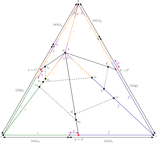
Figure 5. To the proof of Proposition 5.14.

Proposition 5.14.

In a graph $G$ (respectively, a geodesic metric space $X$), for any BFS-tree $T$ (respectively, any GS-tree $T$) rooted at some vertex $w$, $\iota(G)=\tau(G)\leq 7\rho_{w,T}(G)+4$ (respectively, $\iota(X)=\tau(X)\leq 7\rho_{w,T}(X)$).

Proof.

We prove the proposition for graphs (for geodesic spaces, the proof is similar but simpler). Let $\rho:=\rho_{w,T}(G)$. Consider a geodesic triangle $\Delta(x,y,z)=[x,y]\cup[y,z]\cup[z,x]$ and assume without loss of generality that $(x|y)_{w}\leq(y|z)_{w}\leq(x|z)_{w}$. Let $a:=(x|y)_{w}$, $b:=(y|z)_{w}-a$, and $c:=(x|z)_{w}-a-b$. Let $e:=(w|z)_{x}$, $f:=(w|x)_{z}$ and $d:=d(y,w)-(x|z)_{w}=d(y,w)-a-b-c$. See Fig. 5 for an illustration (in this example, $a$ is very small and not represented in the figure). Observe that $d$ may be negative but that $a,b,c,e,f\geq 0$. Note that $b\leq\delta_{w}\leq\rho+\frac{1}{2}$ as explained in the proof of Theorem 5.2. Observe that $d(w,x)=a+b+c+e$, $d(w,y)=a+b+c+d$, $d(w,z)=a+b+c+f$, $d(x,z)=e+f$, $d(y,z)=d+f+2c$, and $d(x,y)=e+d+2b+2c.$

Let $v$ and $u$ be the vertices of $[x,y]$ and $[x,z]$ at distance $\lfloor(y|z)_{x}\rfloor$ from $x$, let $u^{\prime}$ and $t^{\prime}$ be the vertices of $[z,x]$ and $[z,y]$ at distance $\lfloor(x|y)_{z}\rfloor$ from $z$, and let $v^{\prime\prime}$ and $t^{\prime\prime}$ be the vertices of $[y,x]$ and $[y,z]$ at distance $\lfloor(x|z)_{y}\rfloor$ from $y$. In order to prove the proposition, we need to show that $d(u,v),d(u^{\prime},t^{\prime}),d(v^{\prime\prime},t^{\prime\prime})\leq 7\rho+4$.

We first show that $d(u^{\prime},t^{\prime})\leq 4\rho+2$. Let $u^{\prime}_{z}$ and $z_{u^{\prime}}$ be the vertices of $[w,u^{\prime}]$ and $[w,z]$ at distance $\lfloor(u^{\prime}|z)_{w}\rfloor$ from $w$. Let $t^{\prime}_{z}$ and $z_{t^{\prime}}$ be the vertices of $[w,t^{\prime}]$ and $[w,z]$ at distance $\lfloor(t^{\prime}|z)_{w}\rfloor$ from $w$. Note that

$$d(u^{\prime},t^{\prime}) \leq d(u^{\prime},u^{\prime}_{z})+d(u^{\prime}_{z},z_{u^{\prime}})+d(z_{u^{\prime}},z_{t^{\prime}})+d(z_{t^{\prime}},t^{\prime}_{z})+d(t^{\prime}_{z},t^{\prime})$$

$$\leq\lceil(w|z)_{u^{\prime}}\rceil+\rho+d(z_{u^{\prime}},z_{t^{\prime}})+\rho+\lceil(w|z)_{t^{\prime}}\rceil.$$

Observe also that $d(z,z_{t^{\prime}})=d(z,t^{\prime})-\lfloor(w|z)_{t^{\prime}}\rfloor=\lfloor(x|y)_{z}\rfloor-\lfloor(w|z)_{t^{\prime}}\rfloor$ and similarly, $d(z,z_{u^{\prime}})=\lfloor(x|y)_{z}\rfloor-\lfloor(w|z)_{u^{\prime}}\rfloor$. Consequently, $d(z_{u^{\prime}},z_{t^{\prime}})=|\lfloor(w|z)_{u^{\prime}}\rfloor-\lfloor(w|z)_{t^{\prime}}\rfloor|$. Therefore, we have

$$d(u^{\prime},t^{\prime})\leq 2\rho+2\max((w|z)_{u^{\prime}},(w|z)_{t^{\prime}})+1.$$

Notice that $d(z,u^{\prime})=d(z,t^{\prime})\leq(x|y)_{z}=f-b\leq f+c=(w|y)_{z}$. By Lemma 5.13, $(w|z)_{u^{\prime}},(w|z)_{t^{\prime}}\leq\rho+\frac{1}{2}$, and consequently, $d(u^{\prime},t^{\prime})\leq 4\rho+2$.

We now show that $d(u,v)\leq 6\rho+3$. Note that if $b=0$, then we are in the same case as for the pair $u^{\prime},t^{\prime}$, and thus we can assume that $b>0$. Let $u_{x}$ and $x_{u}$ be the vertices of $[w,u]$ and $[w,x]$ at distance $\lfloor(u|x)_{w}\rfloor$ from $w$. Let ${v}_{x}$ and $x_{v}$ be the vertices of $[w,v]$ and $[w,x]$ at distance $\lfloor(v|x)_{w}\rfloor$ from $w$. Observe that

$$d(u,v) \leq d(u,{u}_{x})+d({u}_{x},x_{u})+d(x_{u},x_{v})+d(x_{v},{v}_{x})+d({v}_{x},v)$$

$$\leq\lceil(w|x)_{u}\rceil+\rho+d(x_{u},x_{v})+\rho+\lceil(w|x)_{v}\rceil.$$

Observe also that $d(x,x_{u})=d(x,u)-\lfloor(w|x)_{u}\rfloor=\lfloor(y|z)_{x}\rfloor-\lfloor(w|x)_{u}\rfloor$ and similarly, $d(x,x_{v})=\lfloor(y|z)_{x}\rfloor-\lfloor(w|x)_{v}\rfloor$. Consequently, $d(x_{u},x_{v})=|\lfloor(w|x)_{u}\rfloor-\lfloor(w|x)_{v}\rfloor|$. Therefore, we have

$$d(u,v)\leq 2\rho+2\max((w|x)_{u},(w|x)_{v})+1.$$

Notice that $d(x,v)\leq(y|z)_{x}=e+b\leq e+b+c=(y|w)_{x}$ and that $d(x,u)=\lfloor e+b\rfloor=\lfloor(z|w)_{x}+b\rfloor\geq(z|w)_{x}$ (since $b>0$). By Lemma 5.13, $(w|x)_{v}\leq\rho+\frac{1}{2}$, and $(w|x)_{u}=(w|z)_{u}+(w|x)_{z}-d(u,z)\leq(w|x)_{z}-d(u,z)+\rho+\frac{1}{2}$. Since $(w|x)_{z}=f$ and $d(u,z)=\lceil(x|y)_{z}\rceil=\lceil f-b\rceil$, we have $(w|x)_{u}\leq b+\rho+\frac{1}{2}\leq 2\rho+1$, and consequently, $d(u,v)\leq 6\rho+3$.

We finally show that $d(v^{\prime\prime},t^{\prime\prime})\leq 7\rho+4$. Note that if $c=0$, then we are in the same case as for the pair $u,v$, and we can thus assume that $c>0$. Let $v^{\prime\prime}_{x}$ and $x_{v^{\prime\prime}}$ be the vertices of $[w,v^{\prime\prime}]$ and $[w,x]$ at distance $\lfloor(v^{\prime\prime}|x)_{w}\rfloor$ from $w$. Let $t^{\prime\prime}_{z}$ and $z_{t^{\prime\prime}}$ be the vertices of $[w,t^{\prime\prime}]$ and $[w,z]$ at distance $\lfloor(t^{\prime\prime}|z)_{w}\rfloor$ from $w$. Let $x_{z}$ and $z_{x}$ be the vertices of $[w,x]$ and $[w,z]$ at distance $\lfloor(x|z)_{w}\rfloor$ from $w$.

Observe that

$$d(t^{\prime\prime},v^{\prime\prime}) \leq d(t^{\prime\prime},t^{\prime\prime}_{z})+d(t^{\prime\prime}_{z},z_{t^{\prime\prime}})+d(z_{t^{\prime\prime}},z_{x})+d(z_{x},{x}_{z})+d({x}_{z},x_{v^{\prime\prime}})+d(x_{v^{\prime\prime}},v^{\prime\prime}_{x})+d(v^{\prime\prime}_{x},v^{\prime\prime})$$

$$\leq\lceil(w|z)_{t^{\prime\prime}}\rceil+\rho+d(z_{t^{\prime\prime}},z_{x})+\rho+d({x}_{z},x_{v^{\prime\prime}})+\rho+\lceil(w|x)_{v^{\prime\prime}}\rceil.$$

Notice that $d(z,z_{t^{\prime\prime}})=d(z,t^{\prime\prime})-\lfloor(w|z)_{t^{\prime\prime}}\rfloor=\lceil(x|y)_{z}\rceil-\lfloor(w|z)_{t^{\prime\prime}}\rfloor=\lceil f-b\rceil-\lfloor(w|z)_{t^{\prime\prime}}\rfloor$. Moreover, note that $d(z,z_{x})=\lceil(x|w)_{z}\rceil=\lceil f\rceil$. Consequently, $d(z_{x},z_{t^{\prime\prime}})\leq\lceil b\rceil+\lfloor(w|z)_{t^{\prime\prime}}\rfloor$.

Observe also that $d(x,x_{v^{\prime\prime}})=d(x,v^{\prime\prime})-\lfloor(x|w)_{v^{\prime\prime}}\rfloor=\lceil(y|z)_{x}\rceil-\lfloor(x|w)_{v^{\prime\prime}}\rfloor=\lceil e+b\rceil-\lfloor(x|w)_{v^{\prime\prime}}\rfloor$. Moreover, note that $d(x,x_{z})=\lceil(z|w)_{x}\rceil=\lceil e\rceil$. Consequently, $d(x_{z},x_{v^{\prime\prime}})=|\lceil e+b\rceil-\lfloor(x|w)_{v^{\prime\prime}}\rfloor-\lceil e\rceil|\leq\max(\lceil b\rceil-\lfloor(x|w)_{v^{\prime\prime}}\rfloor,\lfloor(x|w)_{v^{\prime\prime}}\rfloor-\lfloor b\rfloor)$. Therefore, we have

$$d(t^{\prime\prime},v^{\prime\prime}) \leq 3\rho+\lceil(w|z)_{t^{\prime\prime}}\rceil+\lceil b\rceil+\lfloor(w|z)_{t^{\prime\prime}}\rfloor+d(x_{z},x_{v^{\prime\prime}})+\lceil(w|x)_{v^{\prime\prime}}\rceil$$

$$\leq 3\rho+2(w|z)_{t^{\prime\prime}}+\lceil b\rceil+\max(\lceil b\rceil-\lfloor(x|w)_{v^{\prime\prime}}\rfloor,\lfloor(x|w)_{v^{\prime\prime}}\rfloor-\lfloor b\rfloor)+\lceil(w|x)_{v^{\prime\prime}}\rceil$$

$$\leq 3\rho+2(w|z)_{t^{\prime\prime}}+2\max(\lceil b\rceil,(w|x)_{v^{\prime\prime}})+1.$$

Notice that $d(x,v^{\prime\prime})=\lceil(y|z)_{x}\rceil=\lceil e+b\rceil\leq e+b+c=(y|w)_{x}$ (since $c>0$) and $d(z,t^{\prime\prime})=\lceil(x|y)_{z}\rceil=\lceil f-b\rceil\leq f+c$ (since $c>0$). Recall that $f+c=(y|w)_{z}$. Consequently, by Lemma 5.13, $(w|x)_{v^{\prime\prime}},(w|z)_{t^{\prime\prime}}\leq\rho+\frac{1}{2}$. Since $b\leq\rho+\frac{1}{2}$, we get that $d(t^{\prime\prime},v^{\prime\prime})\leq 7\rho+4$. ∎

Consider a collection $\mathcal{T}=(T_{w})_{w\in V}$ of trees where for each $w$, $T_{w}$ is an arbitrary BFS-tree rooted at $w$, and let $\rho_{\mathcal{T}}(G):=\max_{w\in V}\rho_{w,T_{w}}(G)$. Since for each $w$, $\rho_{w,T_{w}}(G)$ can be computed in $O(n^{2})$ time, $\rho_{\mathcal{T}}(G)$ can be computed in $O(n^{3})$ time. We stress that for any fixed $w\in V$, $\delta_{w}(G)$ can be also computed naively in $O(n^{3})$ time and in $O(n^{2.69})$ time using (max,min) matrix product [22]. Furthermore, by Proposition 2.1, $\delta_{w}(G)$ gives a 2-approximation of the hyperbolicity $\delta(G)$ of $G$. In what follows, we present approximation algorithms with similar running times for $\varsigma(G)$ and $\tau(G)$.

To get a better bound for $\varsigma(G)$, we need to involve one more parameter. Let $u$ and $v$ be arbitrary vertices of $G$ and $T_{u}\in\mathcal{T}$ be the BFS-tree rooted at $u$. Let also $(u=u_{0},u_{1},\dots,u_{\ell}=v)$ be the path of $T_{u}$ joining $u$ with $v$. Define $\kappa_{T_{u}}(u,v):=\max\{d(a,u_{i}):a\in I(u,v),d(a,u)=i\}$ and $\kappa_{\mathcal{T}}(G):=\max\{\kappa_{T_{u}}(u,v):u,v\in V\}$. Note that $\kappa_{\mathcal{T}}(G)\leq\kappa(G)$ and that $\kappa_{\mathcal{T}}(G)$ can be computed in $O(n^{3})$ time and $O(n^{2})$ space. Observe also that for any $u,v$, $\kappa_{T_{u}}(u,v)\leq\rho_{u,T_{u}}(G)$ and thus $\kappa_{\mathcal{T}}(G)\leq\rho_{\mathcal{T}}(G)$.

Proposition 5.15.

For a graph $G$ and a collection of BFS-trees $\mathcal{T}=(T_{w})_{w\in V}$, $\iota(G)=\tau(G)\leq\rho_{\mathcal{T}}(G)+2\kappa_{\mathcal{T}}(G)\leq 3\rho_{\mathcal{T}}(G)\leq 3\tau(G)$ and $\varsigma(G)\leq\rho_{\mathcal{T}}(G)+2{\kappa_{\mathcal{T}}(G)}\leq 8\varsigma(G)$. Consequently, a 3-approximation of the thinness $\tau(G)$ and an 8-approximation of the slimness $\varsigma(G)$ can be found in $O(n^{3})$ time and $O(n^{2})$ space.

Proof.

Pick any geodesic triangle $\Delta(x,y,w)$ with sides $[x,y]$, $[x,w]$ and $[y,w]$. Let $[x,w]_{T}$ and $[y,w]_{T}$ be the corresponding geodesics of the BFS-tree $T$ for vertex $w$. Consider the vertices $x_{y}\in[x,w]_{T},y_{x}\in[w,y]_{T}$ and vertices $a\in[x,w],b\in[y,w]$ with $d(w,x_{y})=d(w,y_{x})=d(w,a)=d(w,b)=\lfloor(x|y)_{w}\rfloor$. We know that $d(x_{y},y_{x})\leq\rho_{\mathcal{T}}(G)$. Since $(x|a)_{w}=d(a,w)$ and $(y|b)_{w}=d(b,w)$, $d(a,x_{y})\leq\kappa_{T_{w}}(w,x)\leq\kappa_{\mathcal{T}}(G)$ and $d(b,y_{x})\leq\kappa_{T_{w}}(w,y)\leq\kappa_{\mathcal{T}}(G)$. Hence, $d(a,b)\leq\rho_{\mathcal{T}}(G)+2\kappa_{\mathcal{T}}(G)$. Repeating this argument for vertices $x$ and $y$ and their BFS-trees, we get that the insize of $\Delta(x,y,w)$ is at most $\rho_{\mathcal{T}}(G)+2\kappa_{\mathcal{T}}(G)$. So $\tau(G)\leq\rho_{\mathcal{T}}(G)+2\kappa_{\mathcal{T}}(G)$ and by Proposition 3.1, $\varsigma(G)\leq\tau(G)\leq\rho_{\mathcal{T}}(G)+2\kappa_{\mathcal{T}}(G)\leq\tau(G)+2\kappa(G)\leq 8\varsigma(G)$. ∎

6. Exact computation

In this section, we provide exact algorithms for computing the slimness $\varsigma(G)$, the thinness $\tau(G)$, and the insize $\iota(G)$ of a given graph $G$. The algorithm computing $\tau(G)=\iota(G)$ runs in $O(n^{2}m)$ time and the algorithm computing $\varsigma(G)$ runs in $\widehat{O}(n^{2}m+n^{4}/\log^{3}n)$ time (as we already noticed above, the $\widehat{O}(\cdot)$ notation hides polyloglog factors); both algorithms are combinatorial and use $O(n^{2})$ space. When the graph is dense (i.e., $m=\Omega(n^{2})$), that stays of the same order of magnitude as the best-known algorithms for computing $\delta(G)$ in practice (see [4]), but when the graph is not so dense (i.e., $m=o(n^{2})$), our algorithms run in $o(n^{4})$ time. In contrast to this result, the existing algorithms for computing $\delta(G)$ exactly are not sensitive to the density of the input. We also show that the minsize $\rho_{-}(G)$ of a given graph $G$ cannot be approximated with a factor strictly better than 2 unless P = NP. The main result of this section is the following theorem:

Theorem 6.1.

For a graph $G=(V,E)$ with $n$ vertices and $m$ edges, the following holds:

1. the thinness $\tau(G)$ and the insize $\iota(G)$ of $G$ can be computed in $O(n^{2}m)$ time;

2. the slimness $\varsigma(G)$ of $G$ can be computed in $\widehat{O}(n^{2}m+n^{4}/\log^{3}n)$ time combinatorially and in $O(n^{3.273})$ time using matrix multiplication;

3. deciding whether the minsize $\rho_{-}(G)$ of $G$ is at most $1$ is NP-complete.

One of the difficulties of computing $\varsigma(G),\tau(G),$ and $\iota(G)$ exactly is that these parameters are defined as minima of some functions over all geodesic triangles of the graph, and that there may be exponentially many such triangles. However, even in the case where there are unique shortest paths between all pairs of vertices, our algorithms have a better complexity than the naive algorithms following from the definitions of these parameters.

6.1. Exact computation of thinness and insize

In this subsection, we prove the following result (Theorem 6.1(1)):

Proposition 6.2.

$\tau(G)$ and $\iota(G)$ can be computed in $O(n^{2}m)$ time.

To prove Proposition 6.2, we introduce the “pointed thinness” $\tau_{x}(G)$ of a given vertex $x$. For a fixed vertex $x$, let $\tau_{x}(G)=\max\big{\{}d(y^{\prime},z^{\prime}):\exists y,z\in V\text{ such that }y^{\prime}\in I(x,y),z^{\prime}\in I(x,z),\text{ and }d(x,y^{\prime})=d(x,z^{\prime})\leq(y|z)_{x}\big{\}}$. Observe that for any BFS-tree $T$ rooted at $x$, we have $\rho_{x,T}(G)\leq\tau_{x}(G)\leq\tau(G)$, and thus by Corollary 5.11, $\tau_{x}(G)$ is an 8-approximation (with additive surplus 4) of $\tau(G)$. Since $\tau(G)=\max_{x\in V}\tau_{x}(G)$, given an algorithm for computing $\tau_{x}(G)$ in $O(T(n,m))$ time, we can compute $\tau(G)$ in $O(nT(n,m))$ time, by calling $n$ times this algorithm. Next, we describe such an algorithm that runs in $O(nm)$ time for every $x$. By the remark above, the latter will prove Theorem 6.1(1).

Let $\tau_{x,y}(G):=\max\big{\{}d(y^{\prime},z^{\prime}):y^{\prime}\in I(x,y)\text{ and }\exists z\in V\text{ such that }z^{\prime}\in I(x,z)\text{ and }d(x,y^{\prime})=d(x,z^{\prime})\leq(y|z)_{x}\big{\}}$ and observe that $\tau_{x}(G)=\max_{y\in V}\tau_{x,y}(G)$.

For every ordered pair $x,y$ and every vertex $w$, let $g_{w}(x,y)=\max\big{\{}d(y^{\prime},w):y^{\prime}\in I(x,y)\text{ and }d(x,y^{\prime})=d(x,w)\big{\}}$ and let $h_{x,y}(w)=\max\big{\{}(y|z)_{x}:w\in I(x,z)\big{\}}$. The following lemma is the cornerstone of our algorithm.

Lemma 6.3.

For any $x,y\in V$, $\tau_{x,y}(G)=\max\big{\{}g_{w}(x,y):d(x,w)\leq h_{x,y}(w)\big{\}}$.

Proof.

Let $\beta_{x,y}:=\max\big{\{}g_{w}(x,y):d(x,w)\leq h_{x,y}(w)\big{\}}$ and consider $w$ such that $\beta_{x,y}=g_{w}(x,y)$ and $d(x,w)\leq h_{x,y}(w)$. Consider a vertex $y^{\prime}\in I(x,y)$ such that $d(x,y^{\prime})=d(x,w)$ and $d(y^{\prime},w)=g_{w}(x,y)$. Consider a vertex $z$ such that $w\in I(x,z)$ and $h_{x,y}(w)=(y|z)_{x}$. Since $d(x,y^{\prime})=d(x,w)\leq h_{x,y}(w)=(y|z)_{x}$, $\beta_{x,y}=g_{w}(x,y)=d(y^{\prime},w)\leq\tau_{x,y}(G)$.

Conversely, consider $y^{\prime},z^{\prime},z$ such that $y^{\prime}\in I(x,y)$, $z^{\prime}\in I(x,z)$, $d(x,y^{\prime})=d(x,z^{\prime})\leq(y|z)_{x}$, and $\tau_{x,y}(G)=d(y^{\prime},z^{\prime})$. Observe that $d(y^{\prime},z^{\prime})\leq g_{z^{\prime}}(x,y)$ and that $d(x,z^{\prime})\leq(y|z)_{x}\leq h_{x,y}(z^{\prime})$. Consequently, $\tau_{x,y}(G)=d(y^{\prime},z^{\prime})\leq g_{z^{\prime}}(x,y)\leq\beta_{x,y}$. ∎

The algorithm for computing $\tau_{x}(G)$ works as follows. First, we compute the distance matrix of $G$ in $O(mn)$ time. Next, we compute $g_{w}(x,y)$ and $h_{x,y}(w)$ for all $y,w$ in time $O(mn)$. Finally, we enumerate all $y,w$ in $O(n^{2})$ to compute $\max\big{\{}g_{w}(x,y):d(x,w)\leq h_{x,y}(w)\big{\}}$. By Lemma 6.3, the obtained value is exactly $\tau_{x}(G)=\max\tau_{x,y}(G)$. Therefore, we are just left with proving that we can compute $g_{w}(x,y)$ and $h_{x,y}(w)$ for all $y,w$ in time $O(mn)$, which is a direct consequence of the two next lemmas.

Lemma 6.4.

For any fixed $x,w\in V$, one can compute the values of $g_{w}(x,y)$ for all $y\in V$ in ${O}(m)$ time.

Proof.

In order to compute $g_{w}(x,y)$, we use the following recursive formula: $g_{w}(x,y)=0$ if $d(x,y)<d(x,w)$, $g_{w}(x,y)=d(w,y)$ if $d(x,y)=d(x,w)$, and $g_{w}(x,y)=\max\big{\{}g_{w}(x,y^{\prime}):y^{\prime}\in N(y)\text{ and }d(x,y^{\prime})=d(x,y)-1\big{\}}$ otherwise. Given the distance matrix $D$, for any $y\in V$, we can compute $\{y^{\prime}\in N(y):d(x,y^{\prime})=d(x,y)-1\}$ in ${O}(\deg(y))$ time. Therefore, using a standard dynamic programming approach, we can compute the values $g_{w}(x,y)$ for all $y\in V$ in ${O}(\sum_{y}\deg(y))=O(m)$ time. ∎

Lemma 6.5.

For any fixed $x,y\in V$, one can compute the values of $h_{x,y}(w)$ for all $w\in V$ in ${O}(m)$ time.

Proof.

In order to compute $h_{x,y}(w)$, we use the following recursive formula: $h_{x,y}(w)=\max\big{\{}(y|w)_{x},h^{\prime}_{x,y}(w)\big{\}}$ where $h^{\prime}_{x,y}(w)=\max\big{\{}h_{x,y}(w^{\prime}):w^{\prime}\in N(w)\text{ and }d(x,w^{\prime})=d(x,w)+1\big{\}}$. Given the distance matrix $D$, for any fixed $w\in V$, we can compute $\big{\{}w^{\prime}\in N(w):d(x,w^{\prime})=d(x,w)+1\big{\}}$ in $O(\deg(w))$ time. If we order the vertices of $V$ by non-increasing distance to $x$, using dynamic programming, we can compute the values of $h_{x,y}(w)$ for all $w$ in $O(\sum_{w}\deg(w))=O(m)$ time. ∎

6.2. Exact computation of slimness

The goal of this subsection is to prove the following result (Theorem 6.1(2)):

Proposition 6.6.

$\varsigma(G)$ can be computed in $\widehat{O}(n^{2}m+n^{4}/\log^{3}n)$ time combinatorially and in $O(n^{3.273})$ time using matrix multiplication.

To prove Proposition 6.6, we introduce the “pointed slimness” $\varsigma_{w}(G)$ of a given vertex $w$. Formally, $\varsigma_{w}(G)$ is the least integer $k$ such that, in any geodesic triangle $\Delta(x,y,z)$ such that $w\in[x,y]$, we have $d(w,[x,z]\cup[y,z])\leq k$. Note that $\varsigma_{w}(G)$ cannot be used to approximate $\varsigma(G)$ (that is in sharp contrast with $\delta_{w}(G)$ and $\tau_{w}(G)$). In particular, $\varsigma_{w}(G)=0$ whenever $w$ is a pending vertex (a vertex of degree 1), or, more generally, a simplicial vertex (a vertex whose every two neighbors are adjacent) of $G$. On the other hand, we have $\varsigma(G)=\max_{w\in V}\varsigma_{w}(G)$. Therefore, given an algorithm for computing $\varsigma_{w}(G)$ in $O(T(n,m))$ time, we can compute $\varsigma(G)$ in $O(nT(n,m))$ time, by calling $n$ times this algorithm. Next we describe such an algorithm that is combinatorial and runs in $\widehat{O}(nm+n^{3}/\log^{3}n)$ (Lemma 6.10). We also explain how to compute $\varsigma(G)$ in $O(n^{2.373})$ time using matrix multiplication (Corollary 6.11). By the remark above, it will prove Theorem 6.1(2). For every $y,z\in V$ we set $p_{w}(y,z)$ to be the least integer $k$ such that, for every geodesic $[y,z]$, we have $d(w,[y,z])\leq k$. The following lemma is the cornerstone of our algorithm.

Lemma 6.7.

$\varsigma_{w}(G)\leq k$ iff for all $x,y\in V$ such that $w\in I(x,y)$, and any $z\in V$, $\min\{p_{w}(x,z),p_{w}(y,z)\}\leq k$.

Proof.

In one direction, let $\Delta(x,y,z)$ be any geodesic triangle such that $w\in[x,y]$. Then, $d(w,[x,z]\cup[y,z])\leq\min\{p_{w}(x,z),p_{w}(y,z)\}\leq k$. Since $\Delta(x,y,z)$ is arbitrary, $\varsigma_{w}(G)\leq k$. Conversely, assume that $\varsigma_{w}(G)\leq k$. Let $x,y,z\in V$ be arbitrary vertices such that $w\in I(x,y)$. Consider a geodesic triangle $\Delta(x,y,z)$ by selecting its sides in such a way that $w\in[x,y]$ and $d(w,[x,z])=p_{w}(x,z),d(w,[y,z])=p_{w}(y,z)$ hold. Then $d(w,[x,z]\cup[y,z])=\min\{p_{w}(x,z),p_{w}(y,z)\}\leq\varsigma_{w}(G)\leq k$, and we are done. ∎

The algorithm for computing $\varsigma_{w}(G)$ proceeds in two phases. We first compute $p_{w}(y,z)$ for every $y,z\in V$. Second, we seek for a triplet $(x,y,z)$ of distinct vertices such that $w\in I(x,y)$ and $\min\{p_{w}(x,z),p_{w}(y,z)\}$ is maximized. By Lemma 6.7, the obtained value is exactly $\varsigma_{w}(G)$. Therefore, we are just left with proving the running time of our algorithm.

Lemma 6.8.

The values $p_{w}(y,z)$, for all $y,z\in V$, can be computed in ${O}(nm)$ time.

Proof.

By induction on $d(y,z)$, the following formula holds for $p_{w}(y,z)$: $p_{w}(y,z)=d(w,y)$ if $y=z$; otherwise, $p_{w}(y,z)=\min\{d(w,y),\ \max\{p_{w}(x,z):x\in N(y)\cap I(y,z)\}\}$. Since the distance matrix $D$ of $G$ is available, for any $y,z\in V$ and for any $x\in N(y)$, we can check in constant time whether $x\in I(y,z)$ (i.e., whether $d(x,z)=d(y,z)-1$). In particular, given $y\in V$, for every of the $n$ possible choices for $z$, the intersection $N(y)\cap I(y,z)$ can be computed in ${O}(\deg(y))$ time. Therefore, using a standard dynamic programming approach, all the values $p_{w}(y,z)$ can be computed in time ${O}(nm+\sum_{y}n\cdot\deg(y))$, that is in ${O}(nm)$. ∎

We note that once the distance-matrix of $G$ has been precomputed, and we have all the values $p_{w}(y,z)$, for all $y,z\in V$, then we can compute $\varsigma_{w}(G)$ as follows. We enumerate all possible triplets $(x,y,z)$ of distinct vertices of $G$, and we keep one such that $w\in I(x,y)$ and $\min\{p_{w}(x,z),p_{w}(y,z)\}$ is maximized. It takes $O(n^{3})$ time. In what follows, we shall explain how the running time can be improved by reducing the problem to Triangle Detection. More precisely, let $k$ be a fixed integer. The graph $\Gamma_{\varsigma}[k]$ has vertex set $V_{1}\cup V_{2}\cup V_{3}$, with every set $V_{i}$ being a copy of $V\setminus\{w\}$. There is an edge between $x_{1}\in V_{1}$ and $y_{2}\in V_{2}$ if and only if the corresponding vertices $x,y\in V$ satisfy $w\in I(x,y)$. Furthermore, there is an edge between $x_{1}\in V_{1}$ and $z_{3}\in V_{3}$ (respectively, between $y_{2}\in V_{2}$ and $z_{3}\in V_{3}$) if and only if we have $p_{w}(x,z)>k$ (respectively, $p_{w}(y,z)>k$).

Lemma 6.9.

$\varsigma_{w}(G)\leq k$ if and only if $\Gamma_{\varsigma}[k]$ is triangle-free.

Proof.

By construction there is a bijective correspondence between the triangles $(x_{1},y_{2},z_{3})$ in $\Gamma_{\varsigma}[k]$ and the triplets $(x,y,z)$ such that $w\in I(x,y)$ and $\min\{p_{w}(x,z),p_{w}(y,z)\}>k$. By Lemma 6.7, we have $\varsigma_{w}(G)\leq k$ if and only if there is no triplet $(x,y,z)$ such that $w\in I(x,y)$ and $\min\{p_{w}(x,z),p_{w}(y,z)\}>k$. As a result, $\varsigma_{w}(G)\leq k$ if and only if $\Gamma_{\varsigma}[k]$ is triangle-free. ∎

Lemma 6.10.

For $w\in V$, we can compute $\varsigma_{w}(G)$ in $\widehat{O}(nm+n^{3}/\log^{3}n)$ time combinatorially.

Proof.

We compute the values $p_{w}(y,z)$, for every $y,z\in V$. By Lemma 6.8, it takes time ${O}(nm)$. Furthermore, within the same amount of time, we can also compute the distance matrix $D$ of $G$. Then, we need to observe that given an algorithm to decide whether $\varsigma_{w}(G)\leq k$ for any $k$, that runs in $O(T(n,m))$ time, we can compute $\varsigma_{w}(G)$ in $O(T(n,m)\log n)$ time, simply by performing a one-sided binary search. In what follows, we describe such an algorithm that runs in time $\widehat{O}(n^{3}/\log^{4}n)$. For that, we reduce the problem to Triangle Detection. We construct the graph $\Gamma_{\varsigma}[k]$. Since the values $p_{w}(y,z)$, for all $y,z\in V$, and the distance matrix of $G$ are given, this can be done in ${O}(n^{2})$ time. Furthermore, by Lemma 6.9, $\varsigma_{w}(G)\leq k$ if and only if $\Gamma_{\varsigma}[k]$ is triangle-free. Since Triangle Detection can be solved combinatorially in time $\widehat{O}(n^{3}/\log^{4}n)$ [34], we are done by calling ${O}(\log{n})$ times a Triangle Detection algorithm. ∎

Interestingly, in the proof of Lemma 6.10 we reduced the computation of $\varsigma_{w}(G)$ to a single call to an all-pair-shortest-path algorithm, and to ${O}(\log{n})$ calls to a Triangle Detection algorithm. It is folklore that both problems can be solved in time ${O}(n^{\omega}\log{n})$ and ${O}(n^{\omega})$, respectively, where $\omega<2.373$ is the exponent for square matrix multiplication. Hence, we obtain the following algebraic version of Lemma 6.10:

Corollary 6.11.

For $w\in V$, we can compute $\varsigma_{w}(G)$ in ${O}(n^{\omega}\log{n})$ time.

We stress that Corollary 6.11 implies the existence of an ${O}(n^{\omega+1}\log{n})$-time algorithm for computing the slimness of a graph (since $\omega<2.373$, this algorithm runs in ${O}(n^{3.273})$ time). In sharp contrast to this result, we recall that the best-known algorithm for computing the hyperbolicity runs in time $O(n^{3.69})$ [22].

A popular conjecture is that Triangle Detection and Matrix Multiplication are equivalent. We prove next that under this assumption, the result of Corollary 6.11 is optimal up to polylogarithmic factors:

Proposition 6.12.

Triangle Detection on $n$-vertex graphs can be reduced in time ${O}(n^{2})$ to computing the pointed slimness of a given vertex in a graph with $\Theta(n)$-vertices.

Proof.

Let $G=(V,E)$ be any graph input for Triangle Detection. Suppose without loss of generality that $G$ is tripartite with a valid partition $V_{1},V_{2},V_{3}$ (otherwise, we replace $G$ with $H=(V_{1}\cup V_{2}\cup V_{3},E_{H})$ where $V_{1},V_{2},V_{3}$ are disjoint copies of $V$ and $E_{H}=\{x_{i}y_{j}:xy\in E\ \text{and}\ 1\leq i<j\leq 3\}$). We construct a graph $G^{*}$ from $G$, as follows.

• For every $v\in V$, there is a path $(v^{-},v^{*},v^{+})$. We so have three copies of the partition sets $V_{i}$, $1\leq i\leq 3$, that we denote by $V_{i}^{-},V_{i}^{*},V_{i}^{+}$.

• For every $xz\in E$ such that $x\in V_{1},z\in V_{3}$, we add an edge $x^{-}z^{+}$. In the same way, for every $yz\in E$ such that $y\in V_{2},z\in V_{3}$, we add an edge $y^{+}z^{-}$. However, for every $x\in V_{1},y\in V_{2}$ we add an edge $x^{+}y^{-}$ if and only if $xy\notin E$.

• We also add two new vertices $\alpha,\beta$ and the edges $\{\alpha x^{*}:x\in V_{1}\}\cup\{\beta y^{*}:y\in V_{2}\}$.

• Finally, we add two more vertices $a,b$ and the edges $\{ab,a\alpha,a\beta\}\cup\{ax^{+},bx^{-}:x\in V_{1}\}\cup\{ay^{-},by^{+}:y\in V_{2}\}\cup\{bz^{-},bz^{+}:z\in V_{3}\}$.

The resulting graph $G^{*}$ has ${O}(n)$ vertices and it can be constructed in ${O}(n^{2})$-time (for an illustration, see Fig. 6). In what follows, we prove that $\varsigma_{a}(G^{*})\geq 2$ if and only if $G$ contains a triangle.

First we assume that $G$ contains a triangle $xyz$ where $x\in V_{1},y\in V_{2},z\in V_{3}$. By construction, the paths $(x^{*},x^{-},z^{+},z^{*})$ and $(z^{*},z^{-},y^{+},y^{*})$ are geodesics and they do not intersect $N_{G^{*}}[a]$. Furthermore, since $xy\in E$, we cannot find any two neighbors of $x^{*}$ and $y^{*}$, respectively, that are adjacent, thereby implying $d_{G^{*}}(x^{*},y^{*})=4$ (e.g., $(x^{*},x^{+},a,y^{-},y^{*})$ is a geodesic). Overall, the triplet $x^{*},y^{*},z^{*}$ is such that $a\in I(x^{*},y^{*})$, $p_{a}(x^{*},z^{*})=p_{a}(y^{*},z^{*})=2$. As a result, $\varsigma_{a}(G^{*})\geq 2$.

Conversely, assume $\varsigma_{a}(G^{*})\geq 2$. Let $r,s,t\in V(G^{*})$ such that: $a\in I(r,s)$, $p_{a}(r,t)\geq 2$ and in the same way $p_{a}(s,t)\geq 2$. We claim that $r=x^{*}$ for some $x\in V$. Indeed, suppose by way of contradiction that this is not the case. By the hypothesis $r\notin N_{G^{*}}[a]$, and so, $r\in\{v^{+},v^{-}\}$ for some $v\in V$ and $r\in N_{G^{*}}(b)$. Furthermore, $d_{G^{*}}(r,a)=2$, and so, since $a\in I(r,s)$ and by the hypothesis $s\notin N_{G^{*}}[a]$, $d_{G^{*}}(r,s)\geq 4$. However, by construction every vertex of $G^{*}$ is at a distance $\leq 2$ from vertex $b$. Since $b\in N_{G^{*}}(r)$, this implies that $r$ has eccentricity at most three, a contradiction. Therefore, we proved as claimed that $r=x^{*}$ for some $x\in V$. We can prove similarly that $s=y^{*}$ for some $y\in V$. Then, observe that we cannot have $x,y\in V_{1}$ (otherwise, $(x^{*},\alpha,y^{*})$ is a geodesic, $d_{G^{*}}(r,s)=d_{G^{*}}(x^{*},y^{*})=2$ and $a\notin I(r,s)$); we cannot have $x,y\in V_{2}$ either. Finally, we cannot have $x\in V_{3}$ for then we would get $d_{G^{*}}(x^{*},a)+d_{G^{*}}(a,y^{*})\geq 3+2=5>4\geq d_{G^{*}}(x^{*},y^{*})$; for the same reason, we cannot have $y\in V_{3}$. Overall, we may assume without loss of generality that $x\in V_{1},y\in V_{2}$. Note that $xy\notin E$ (otherwise, $d_{G^{*}}(x^{*},y^{*})=3$ and $a\notin I(x^{*},y^{*})$). Let $P$ be a shortest $(x^{*},t)$-path and $Q$ be a shortest $(y^{*},t)$-path such that $d_{G^{*}}(a,P)\geq 2,\ d_{G^{*}}(a,Q)\geq 2$. Since $V_{3}^{*}\cup N_{G^{*}}[a]$ intersects any path from $V_{1}^{*}$ to $V_{2}^{*}$, there exists $z\in V_{3}$ such that $z^{*}\in P\cup Q$. By symmetry, we may assume $z^{*}\in P$. It follows from the construction of $G^{*}$ that the unique shortest $(x^{*},z^{*})$-path that does not intersect $N_{G^{*}}[a]$, if any, must be $(x^{*},x^{-},z^{+},z^{*})$. In particular, $xz\in E$. Suppose by contradiction $t\neq z^{*}$. Then, $(x^{*},x^{-},z^{+},z^{*},z^{-})$ is a subpath of $P$, that is impossible because $d_{G^{*}}(x^{*},z^{-})=3$. Therefore, $t=z^{*}$. We prove similarly as before that $yz\in E$. Summarizing, $xyz$ is a triangle of $G$. ∎

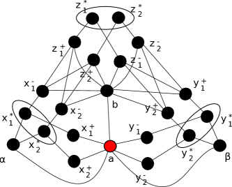
Figure 6. The graph $G^{*}$ obtained from a tripartite graph $G$ and used in the proof of Proposition 6.12.

6.3. Approximating the minsize is hard

In this subsection we prove that, at the difference from other hyperbolicity parameters, deciding whether $\rho_{-}(G)\leq 1$ is NP-complete (Theorem 6.1(3)). Note that since $\rho_{-}(G)$ is an integer, this immediately implies that we cannot find a $(2-\epsilon)$-approximation algorithm to compute $\rho_{-}(G)$ unless P = NP.

Proposition 6.13.

Deciding if $\rho_{-}(G)\leq 1$ is NP-complete.

Note that if we are given a BFS-tree $T$ rooted at $w$, we can easily check whether $\rho_{w,T}(G)\leq 1$, and thus deciding whether $\rho_{-}(G)\leq 1$ is in NP. In order to prove that this problem is NP-hard, we do a reduction from Sat.

Let $\Phi$ be a Sat formula with $m$ clauses $c_{1},c_{2},\ldots,c_{m}$ and $n$ variables $x_{1},x_{2},\ldots,x_{n}$. Up to preprocessing the formula, we can suppose that $\Phi$ satisfies the following properties (otherwise, $\Phi$ can be reduced to a formula satisfying these conditions):

• no clause $c_{j}$ can be reduced to a singleton;

• every literal $x_{i},\overline{x}_{i}$ is contained in at least one clause;

• no clause $c_{j}$ can contain both $x_{i},\overline{x}_{i}$;

• no clause $c_{j}$ can be strictly contained in another clause $c_{k}$;

• every clause $c_{j}$ is disjoint from some other clause $c_{k}$ (otherwise, a trivial satisfiability assignment for $\Phi$ is to set true every literal in $c_{j}$);

• if two clauses $c_{j},c_{k}$ are disjoint, then there exists another clause $c_{p}$ that intersects $c_{j}$ in exactly one literal, and similarly, that also intersects $c_{k}$ in exactly one literal (otherwise, we add the two new clauses $x\vee\overline{y}$ and $\overline{x}\vee y$, with $x,y$ being fresh new variables; then, we replace every clause $c_{j}$ by the two new clauses $c_{j}\vee x\vee y$ and $c_{j}\vee\overline{x}\vee\overline{y}$).

Let $X:=\{x_{1},\overline{x}_{1},\ldots,x_{n},\overline{x}_{n}\}$. For simplicity, in what follows, we often denote $x_{i},\overline{x}_{i}$ by ${\ell}_{2i-1},{\ell}_{2i}$. Let $C:=\{c_{1},\ldots,c_{m}\}$ be the clause-set of $\Phi$. Finally, let $w$ and $V=\{v_{1},v_{2},\ldots,v_{2n}\}$ be additional vertices. We construct a graph $G_{\Phi}$ with $V(G_{\Phi})=\{w\}\cup V\cup X\cup C$ and where $E(G_{\Phi})$ is defined as follows:

• $N(w)=V$ and $V$ is a clique,

• for every $i,i^{\prime}$, $v_{i}$ and ${\ell}_{i^{\prime}}$ are adjacent if and only if $i=i^{\prime}$;

• for every $i,i^{\prime}$, ${\ell}_{i}$ and ${\ell}_{i^{\prime}}$ are adjacent if and only if ${\ell}_{i^{\prime}}\neq\overline{\ell}_{i}$;

• for every $i,j$, $v_{i}$ and $c_{j}$ are not adjacent;

• for every $i,j$, ${\ell}_{i}$ and $c_{j}$ are adjacent if and only if ${\ell}_{i}\in c_{j}$;

• for every $j,j^{\prime}$, $c_{j},c_{j^{\prime}}$ are adjacent if and only if $c_{j},c_{j^{\prime}}$ intersect in exactly one literal.

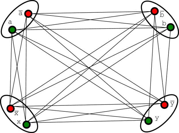
(a) Edges between literal vertices.

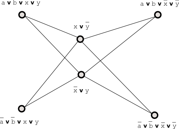
(b) Edges between clause vertices.

(c) Edges between consecutive layers.

(d) A BFS tree $T$ rooted at $w$ s.t. $\rho_{w,T}(G_{\Phi})=1$.

Figure 7. The graph $G_{\Phi}$ obtained from the formula $\Phi=(a\vee b)\land(\bar{a}\vee\bar{b})$. After preprocessing $\Phi$, we got the equivalent formula $(a\vee b\vee x\vee y)\land(a\vee b\vee\bar{x}\vee\bar{y})\land(\bar{a}\vee\bar{b}\vee x\vee y)\land(\bar{a}\vee\bar{b}\vee\bar{x}\vee\bar{y})\land(\bar{x}\vee y)\land(x\vee\bar{y})$.

We refer to Fig. 7 for an illustration.

Proposition 6.14.

${\rho}_{-}(G_{\Phi})\leq 1$ if and only if $\Phi$ is satisfiable.

In order to prove the hardness result, we start by showing that in order to get $\rho_{r,T}(G_{\Phi})\leq 1$ we must have $r=w$. In the following proofs, by a parent node of a node we mean its parent in a BFS-tree $T$.

Lemma 6.15.

For every BFS-tree $T$ rooted at $c_{j}\in C$, we have $\rho_{c_{j},T}(G_{\Phi})\geq 2$.

Proof.

Suppose for the sake of contradiction that we have $\rho_{c_{j},T}(G_{\Phi})\leq 1$. Let $X_{j}\subseteq X$ be the literals in $c_{j}$. Note that since $|X_{j}|>1$, every vertex in $\overline{X}_{j}$ is at distance two from $c_{j}$. We claim that for every ${\ell}_{i^{\prime}}\in\overline{X}_{j}$, the parent node of ${\ell}_{i^{\prime}}$ is in $X_{j}$. Indeed, otherwise this would be some clause-vertex $c_{k}$ such that ${\ell}_{i^{\prime}}\in c_{k}$ and $c_{k}\cap c_{j}\neq\emptyset$. Then, let ${\ell}_{i}\in c_{j}\setminus c_{k}$. Vertex ${\ell}_{i}$ must be the parent node of $v_{i}$. However, $(v_{i}|{\ell}_{i^{\prime}})_{c_{j}}=(2+2-2)/2=1$. The latter implies that $c_{k},{\ell}_{i}$ should be adjacent, that contradicts the fact that ${\ell}_{i}\notin c_{k}$. Therefore, the claim is proved.

Then, let $c_{k}$ be disjoint from $c_{j}$. By construction, $d(c_{j},c_{k})=2$, and the parent node of $c_{k}$ must be some $c_{p}$ such that $c_{j}\cap c_{p}\neq\emptyset$, and similarly $c_{p}\cap c_{k}\neq\emptyset$. Let ${\ell}_{i^{\prime}}\in c_{j}\cap c_{p}$. Furthermore, let ${\ell}_{i}\in c_{j}$ be the parent node of its negation $\overline{\ell}_{i^{\prime}}$ in $T$. We stress that ${\ell}_{i}\notin c_{p}$ since ${\ell}_{i^{\prime}}$ is the unique literal contained in $c_{j}\cap c_{p}$. We have $(c_{k}|\overline{\ell}_{i^{\prime}})_{c_{j}}=2-d(c_{k},\overline{\ell}_{i^{\prime}})/2\in\{1,3/2\}$. In particular, $\lfloor(c_{k}|\overline{\ell}_{i^{\prime}})_{c_{j}}\rfloor=1$. As a result, $\rho_{c_{j},T}(G_{\Phi})\geq d(c_{p},{\ell}_{i})=2$. ∎

Lemma 6.16.

For every BFS-tree $T$ rooted at ${\ell}_{i}\in X$, we have $\rho_{{\ell}_{i},T}(G_{\Phi})\geq 2$.

Proof.

Suppose for the sake of contradiction that $\rho_{{\ell}_{i},T}(G_{\Phi})\leq 1$. Since there is a perfect matching between $X$ and $V=N(w)$, the parent node of $w$ must be $v_{i}$. We claim that the parent node of $v_{i^{\prime}}$, for every $i^{\prime}\neq i$, must be also $v_{i}$. Indeed, otherwise this should be ${\ell}_{i^{\prime}}$. However, $(w|v_{i^{\prime}})_{{\ell}_{i}}=(2+2-1)/2=3/2$. In particular, $\lfloor(w|v_{i^{\prime}})_{{\ell}_{i}}\rfloor=1$, and so, $\rho_{{\ell}_{i},T}(G_{\Phi})\leq 1$ implies $v_{i}$ and ${\ell}_{i^{\prime}}$ should be adjacent, that is a contradiction. So, the claim is proved.

Then, let $c_{j}\in C$ be nonadjacent to ${\ell}_{i}$. We have $d(c_{j},{\ell}_{i})=2$, and the parent node $p_{j}$ of $c_{j}$ must be in $X\cup C$. Let ${\ell}_{i^{\prime}}\in c_{j}$ (possibly, $p_{j}={\ell}_{i^{\prime}}$). We have $(c_{j}|v_{i^{\prime}})_{{\ell}_{i}}=(2+2-2)/2=1$. So, $\rho_{{\ell}_{i},T}(G_{\Phi})\geq d(v_{i},p_{j})=2$. ∎

Lemma 6.17.

For every BFS-tree $T$ rooted at $v_{i}\in V$, we have $\rho_{v_{i},T}(G_{\Phi})\geq 2$.

Proof.

There exists $i^{\prime}\neq i$ such that ${\ell}_{i},{\ell}_{i^{\prime}}$ are nonadjacent. In particular, the parent of ${\ell}_{i^{\prime}}$ must be $v_{i^{\prime}}$. Furthermore, there exists $c_{j}\in C$ such that $d(v_{i},c_{j})=2$. In particular, ${\ell}_{i}$ must be the parent of $c_{j}$. However, $({\ell}_{i^{\prime}}|c_{j})_{v_{i}}=2-d({\ell}_{i^{\prime}},c_{j})/2\in\{1,3/2\}$. In particular, $\lfloor({\ell}_{i^{\prime}}|c_{j})_{v_{i}}\rfloor=1$. So, $\rho_{v_{i},T}(G_{\Phi})\geq d(v_{i^{\prime}},{\ell}_{i})=2$. ∎

From now on, let $w$ be the basepoint of $T$. We prove that for most pairs $s$ and $t$, $d(s_{t},t_{s})\leq 1$ always holds (i.e., regardless whether $\Phi$ is satisfiable).

Lemma 6.18.

If $s\in V$ and $t$ is arbitrary, then $d(s_{t},t_{s})\leq 1$.

Proof.

Since $w$ is a simplicial vertex and $s\in N(w)$, we have $d(w,t)-1\leq d(s,t)\leq d(w,t)$, and consequently,

$$(s|t)_{w}=(d(s,w)+d(t,w)-d(s,t))/2=1/2+(d(t,w)-d(s,t))/2\in\{1/2,1\}.$$

In particular, $s_{t},t_{s}\in N[w]$, and so, $d(s_{t},t_{s})\leq 1$ since $w$ is simplicial. ∎

Lemma 6.19.

If $s,t\in X$, then $d(s_{t},t_{s})\leq 1$.

Proof.

We have $(s|t)_{w}=2-d(s,t)/2$. In particular, $\lfloor(s|t)_{w}\rfloor\leq 1$. As a result, $s_{t},t_{s}\in N[w]$, and since $w$ is simplicial, we obtain $d(s_{t},t_{s})\leq 1$. ∎

Lemma 6.20.

If $s\in X$ and $t\in C$, then $d(s_{t},t_{s})\leq 1$.

Proof.

We have $(s|t)_{w}=5/2-d(s,t)/2\in\{3/2,2\}$. In particular, if $d(s,t)=2$ then $\lfloor(s|t)_{w}\rfloor=1$, and so, we are done because $s_{t},t_{s}\in N[w]$ and $w$ is simplicial. Otherwise, $d(s,t)=1$, and so, $(s|t)_{w}=2$. In particular, $s_{t}=s$ and $s_{t},t_{s}$ are two literals contained in $t$. The latter implies $d(s_{t},t_{s})\leq 1$ since a clause cannot contain a literal and its negation. ∎

Finally, we prove that in order to get $\rho_{w,T}(G_{\Phi})\leq 1$, a necessary and sufficient condition is that the parent nodes in $T$ of the clause vertices are pairwise adjacent in $G_{\Phi}$. By construction, the latter corresponds to a satisfying assignment for $\Phi$.

Lemma 6.21.

If $s,t\in C$, then $s_{t},t_{s}\in X$.

Proof.

We have $(s|t)_{w}=3-d(s,t)/2\in\{2,5/2\}$. In particular, $\lfloor(s|t)_{w}\rfloor=2$. ∎

Acknowledgements

We are grateful to the referees of the journal and short versions of the paper for a careful reading and many useful comments and suggestions. The research of J.C., V.C., and Y.V. was supported by ANR project DISTANCIA (ANR-17-CE40-0015).

References

- [1] M. Abu-Ata and F.F. Dragan. Metric tree-like structures in real-world networks: an empirical study. Networks, 67:49–68, 2016.
- [2] A.B. Adcock, B.D. Sullivan, and M.W. Mahoney. Tree-like structure in large social and information networks. In ICDM 2013, pages 1–10. IEEE Computer Society, 2013.
- [3] J.M. Alonso, T. Brady, D. Cooper, V. Ferlini, M. Lustig, M. Mihalik, M. Shapiro, and H. Short. Notes on word hyperbolic groups. In E. Ghys, A. Haefliger, and A. Verjovsky, editors, Group Theory from a Geometrical Viewpoint, ICTP Trieste 1990, pages 3–63. World Scientific, 1991.
- [4] M. Borassi, D. Coudert, P. Crescenzi, and A. Marino. On computing the hyperbolicity of real-world graphs. In ESA 2015, volume 9294 of Lecture Notes in Comput. Sci., pages 215–226. Springer, 2015.
- [5] M. Borassi, P. Crescenzi, and M. Habib. Into the square: on the complexity of some quadratic-time solvable problems. Electron. Notes Theor. Comput. Sci., 322:51–67, 2016. ICTCS 2015.
- [6] B.H. Bowditch. Notes on Gromov’s hyperbolicity criterion for path-metric spaces. In E. Ghys, A. Haefliger, and A. Verjovsky, editors, Group Theory from a Geometrical Viewpoint, ICTP Trieste 1990, pages 64–167. World Scientific, 1991.
- [7] M.R. Bridson and A. Haefliger. Metric Spaces of Non-Positive Curvature, volume 319 of Grundlehren Math. Wiss. Springer-Verlag, Berlin, 1999.
- [8] J. Chalopin, V. Chepoi, F.F. Dragan, G. Ducoffe, A. Mohammed, and Y. Vaxès. Fast approximation and exact computation of negative curvature parameters of graphs. In SoCG 2018, volume 99 of LIPIcs, pages 22:1–22:15. Schloss Dagstuhl - Leibniz-Zentrum fuer Informatik, 2018.
- [9] J. Chalopin, V. Chepoi, P. Papasoglu, and T. Pecatte. Cop and robber game and hyperbolicity. SIAM J. Discrete Math., 28:1987–2007, 2014.
- [10] V. Chepoi, F.F. Dragan, B. Estellon, M. Habib, and Y. Vaxès. Diameters, centers, and approximating trees of delta-hyperbolic geodesic spaces and graphs. In SoCG 2008, pages 59–68. ACM, 2008.
- [11] V. Chepoi, F.F. Dragan, B. Estellon, M. Habib, Y. Vaxès, and Yang Xiang. Additive spanners and distance and routing labeling schemes for hyperbolic graphs. Algorithmica, 62:713–732, 2012.
- [12] V. Chepoi, F.F. Dragan, and Y. Vaxès. Core congestion is inherent in hyperbolic networks. In SODA 2017, pages 2264–2279. SIAM, 2017.
- [13] V. Chepoi and B. Estellon. Packing and covering -hyperbolic spaces by balls. In APPROX-RANDOM 2007, volume 4627 of Lecture Notes in Comput. Sci., pages 59–73. Springer, 2007.
- [14] N. Cohen, D. Coudert, and A. Lancin. On computing the Gromov hyperbolicity. ACM J. Exp. Algorithmics, 20:1.6:1–1.6:18, 2015.
- [15] D. Coudert and G. Ducoffe. Recognition of -free and -hyperbolic graphs. SIAM J. Discrete Math., 28:1601–1617, 2014.
- [16] D. Coudert, G. Ducoffe, and A. Popa. Fully polynomial FPT algorithms for some classes of bounded clique-width graphs. In SODA 2018, pages 2765–2784. SIAM, 2018.
- [17] B. DasGupta, M. Karpinski, N. Mobasheri, and F. Yahyanejad. Effect of Gromov-hyperbolicity parameter on cuts and expansions in graphs and some algorithmic implications. Algorithmica, 80:772–800, 2018.
- [18] T. Delzant and M. Gromov. Courbure mésoscopique et théorie de la toute petite simplification. J. Topol., 1:804–836, 2008.
- [19] R. Duan. Approximation algorithms for the Gromov hyperbolicity of discrete metric spaces. In LATIN 2014, volume 8392 of Lecture Notes in Comput. Sci., pages 285–293. Springer, 2014.
- [20] K. Edwards, W.S. Kennedy, and I. Saniee. Fast approximation algorithms for -centers in large -hyperbolic graphs. Algorithmica, 80:3889–3907, 2018.
- [21] T. Fluschnik, C. Komusiewicz, G.B. Mertzios, A. Nichterlein, R. Niedermeier, and N. Talmon. When can graph hyperbolicity be computed in linear time? In WADS 2017, volume 10389 of Lecture Notes in Comput. Sci., pages 397–408. Springer, 2017.
- [22] H. Fournier, A. Ismail, and A. Vigneron. Computing the Gromov hyperbolicity of a discrete metric space. Inform Process. Lett., 115:576–579, 2015.
- [23] E. Ghys and P. de la Harpe (eds). Les groupes hyperboliques d’après M. Gromov, volume 83 of Progr. Math. Birkhäuser, 1990.
- [24] M. Gromov. Hyperbolic groups. In S. Gersten, editor, Essays in Group Theory, volume 8 of Math. Sci. Res. Inst. Publ., pages 75–263. Springer, New York, 1987.
- [25] M.F. Hagen. Weak hyperbolicity of cube complexes and quasi-arboreal groups. J. Topology, 7(2):385–418, 2014.
- [26] W.S. Kennedy, I. Saniee, and O. Narayan. On the hyperbolicity of large-scale networks and its estimation. In BigData 2016, pages 3344–3351. IEEE, 2016.
- [27] O. Narayan and I. Saniee. Large-scale curvature of networks. Phys. Rev. E, 84:066108, 2011.
- [28] P. Papasoglu. Strongly geodesically automatic groups are hyperbolic. Invent. Math., 121(2):323–334, 1995.
- [29] P. Papasoglu. An algorithm detecting hyperbolicity. In Geometric and computational perspectives on infinite groups (Minneapolis, MN and New Brunswick, NJ, 1994), volume 25 of DIMACS - Series in Discrete Mathematics and Theoretical Computer Science, pages 193–200. 1996.
- [30] N. Polat. On infinite bridged graphs and strongly dismantlable graphs. Discrete Math., 211:153–166, 2000.
- [31] Y. Shavitt and T. Tankel. Hyperbolic embedding of Internet graph for distance estimation and overlay construction. IEEE/ACM Trans. Netw., 16(1):25–36, 2008.
- [32] M. Soto. Quelques propriétés topologiques des graphes et applications à Internet et aux réseaux. PhD thesis, Université Paris Diderot, 2011.
- [33] K. Verbeek and S. Suri. Metric embedding, hyperbolic space, and social networks. In SoCG 2014, pages 501–510. ACM, 2014.
- [34] H. Yu. An improved combinatorial algorithm for boolean matrix multiplication. In ICALP 2015, volume 9134 of Lecture Notes in Comput. Sci., pages 1094–1105. Springer, 2015.