3D modelling of macroscopic force-free effects in superconducting thin films and rectangular prisms.

Abstract

When the magnetic field has a parallel component to the current density ${\bf J}$ there appear force-free effects due to flux cutting and crossing. This results in an anisotropic ${\bf E}({\bf J})$ relation, being ${\bf E}$ the electric field. Understanding force-free effects is interesting not only for the design of superconducting power and magnet applications but also for material characterization.

This work develops and applies a fast and accurate computer modeling method based on a variational approach that can handle force-free anisotropic ${\bf E}({\bf J})$ relations and perform fully three dimensional (3D) calculations. We present a systematic study of force-free effects in rectangular thin films and prisms with several finite thicknesses under applied magnetic fields with arbitrary angle $\theta$ with the surface. The results are compared with the same situation with isotropic ${\bf E}({\bf J})$ relation.

The thin film situation shows gradual critical current density penetration and a general increase of the magnitude of the magnetization with the angle $\theta$ but a minimum at the remnant state of the magnetization loop. The prism model presents current paths with 3D bending for all angles $\theta$. The average current density over the thickness agrees very well with the thin film model except for the highest angles. The prism hysteresis loops reveal a peak after the remnant state, which is due to the parallel component of the self-magnetic-field and is implicitly neglected for thin films.

The presented numerical method shows the capability to take force-free situations into account for general 3D situations with a high number of degrees of freedom. The results reveal new features of force-free effects in thin films and prisms.

I Introduction

Type II superconductors are essential for large bore or high-field magnets Larbalestier et al. (2014); Kim et al. (2017); Park et al. (2018); Liu and Li (2016) and are promising for power applications, such as motors for air-plane Masson et al. (2007, 2013) or ship propulsion Yanamoto et al. (2017); Gamble et al. (2011), generatorsJeong et al. (2017); Abrahamsen et al. (2010); sup , grid power-transmission cables Volkov et al. (2012); Yagi et al. (2015), transformers Hellmann et al. (2017); Glasson et al. (2017); Schwenterly et al. (1999); Mehta (2011), and or fault-current limiters Pascal et al. (2017); Xin et al. (2013); Morandi (2013); Šouc et al. (2012); Kozak et al. (2016). The Critical Current Density, ${J_{c}}$, of type II superconductors depends on the magnitude and angle of the local magnetic field. There are three types of anisotropy which we call “intrinsic”, “de-pinning”, and “force free” anisotropy.

The “intrinsic” anisotopy is the following. Certain superconductors present an axis with suppressed superconductivity, where the critical current density is lower. In cuprates, for instance, the critical current density in the $c$ crystallographic axis is much smaller than in the $ab$ plane. There is also important anisotropy in REBCO vicinal films due to flux channeling Durrell et al. (2003); Lao et al. (2017).

The “de-pinning” anisotropy of ${J_{c}}$ is due to anisotropic maximum pinning forces caused by either anisotropic pinning centres or anisotropic vortex cores Blatter et al. (1994). When the current density ${{\bf J}}$ is perpendicular to ${{\bf B}}$ and the electric field ${{\bf E}}$ is parallel to ${{\bf J}}$, the anisotropy of ${J_{c}}$ is always due to de-pinning anisotropy. This kind of anisotropy is important for High-Temperature Superconductors (HTS), such as (Bi,Pb)₂Sr₂Ca₂Cu₃O₁₀ and $RE$Ba₂Cu₃O_7-x, and iron-based superconductors. The magnetic field dependence and anisotropy has an impact on the performance of magnets and power applications.

Another type of anisotropy is the “force-free” anisotropy, which appears when the current density presents a substantial parallel component with the local magnetic field. The parallel ${{\bf J}}$ component does not contribute to the macroscopic driving force (or Lorentz force) on the vortices, ${{\bf F}={\bf J}\times{\bf B}}$, being the microscopic vortex dynamics for ${{\bf B}\parallel{\bf J}}$ a complex process that includes flux cutting and crossing Vlasko-Vlasov et al. (2015); Clem (1982); Clem et al. (2011). Many power applications with rotating applied fields are influenced with force-free effects. In principle, the force-free anisotropy also appears for intrinsically isotropic materials.

There are many macroscopical physical models on force-free anisotropy that regard both flux cutting and de-pinning, such as the Double Critical State ModelClem (1982), the General Double Critical State ModelClem and Perez-Gonzalez (1984), Brant and Mikitik Extended Double Critical State Model Brandt and Mikitik (2007) and the Elliptic Critical State Model Romero-Salazar and Pérez-Rodríguez (2003). A valuable comparison of these models can be found in Clem et al. (2011). There are many experimental works on de-pinning anisotropy, such as state of the art REBCO commercial tapes Chepikov et al. (2017); Iijima et al. (2015); Lee et al. (2014); Rossi et al. (2016); Xu et al. (2017); Lin et al. (2017); Miura et al. (2017), Bi2223 tapes Ayai et al. (2008); Goyal et al. (1997) and iron based Pallecchi et al. (2015); Yi et al. (2017); Ma et al. (2017); Hecher et al. (2018) conductors, as well as a database of anisotropic $J_{c}$ measurements HTS . Correction of self-magnetic field in critical current, $I_{c}$, measurements is also important Pardo et al. (2011); Zermeno et al. (2016).

In this article, we focus on force-free effects, which cause anisotropy when ${{\bf J}}$ has a parallel component to ${{\bf B}}$ (or ${{\bf E}}$ is not parallel to ${{\bf J}}$). We also base our study in modelling only. The object of study are thin films and rectangular prisms of several thickness with various angles of the applied fields, with a especial focus on the current path and hysteresis loops. We compared results with the isotropic situation, in order to understand the observed behavior. The modelling is performed by Minimum Electro-Magnetic Entropy Production in 3D Pardo and Kapolka (2017a), which is suitable for 3D calculations, and avoids spending variables in the air. Moreover, the method enables force-free anisotropic power laws Badía-Majós and López (2015), which is the core of this study.

II Mathematical model

II.1 MEMEP 3D method

This study is based on the Minimum ElectroMagnetic Entropy Production in 3D (MEMEP 3D) Pardo and Kapolka (2017a), which is a variational method. The method solves the effective magnetization ${{\bf T}}$, defined as

$$\ \nabla\times{\bf T}={\bf J},$$ (1)

where ${{\bf J}}$ is the current density. In addition to the magnetization case, MEMEP 3D can also take transport currents into account, after adding an extra term in (1) (see Pardo and Kapolka (2017a)). We take the interpretation that ${{\bf T}}$ is an effective magnetization due to the screening currents. The ${{\bf T}}$ vector is non-zero only inside the sample, and hence the method avoids discretization of the air around the sample. The advantages of MEMEP 3D are reduction of computing time, enabling an increase of total number of degrees of freedom in the sample volume, and efficient parallelization. The general equation of electric field ${{\bf E}}$ is derived from Maxwell equations

$$\ {\bf E}({\bf J})=-\dot{\bf A}-\nabla\phi,$$ (2)

$$\ \nabla\cdot{\bf J}=0,$$ (3)

where ${\phi}$ is the scalar potential.

In the Coulomb’s gauge, we can split the vector potential ${{\bf A}}$ to ${{\bf A}_{a}}$ and ${{\bf A}_{J}}$, where ${{\bf A}_{a}}$ is the vector potential contributed by the applied field and ${{\bf A}_{J}}$ is the vector potential contributed by the current density inside the sample. Then, ${{\bf A}_{J}}$ is

$$\ {\bf A}_{J}({\bf r})=\frac{\mu_{0}}{4\pi}\int_{V}d^{3}{{\bf r}^{\prime}}\frac{{\bf J}({\bf r}^{\prime})}{|{\bf r}-{\bf r}^{\prime}|}=\frac{\mu_{0}}{4\pi}\int_{V}d^{3}{{\bf r}^{\prime}}\frac{\nabla^{\prime}\times{\bf T}({\bf r}^{\prime})}{|{\bf r}-{\bf r}^{\prime}|},$$ (4)

where ${{\bf r}}$ and ${{\bf r}^{\prime}}$ are position vectors.

According to the definition of ${{\bf T}}$, we can rewrite equations (2) and (3) into

$$\ {\bf E}(\nabla\times{\bf T})=-\dot{\bf A}-\nabla\phi,$$ (5)

$$\ \nabla\cdot\left(\nabla\times{\bf T}\right)=0.$$ (6)

The second equation is always satisfied, and hence we must solve only the first equation. As it was shown in Pardo and Kapolka (2017a), minimizing the following functional, is the same as solving equation (5).

The functional is

$$\ L_{T}=\int_{V}d^{3}{\bf r}\left[\frac{1}{2}\frac{\Delta{{\bf A}}_{J}}{\Delta t}\cdot(\nabla\times\Delta{\bf T})+\frac{\Delta{{\bf A}}_{a}}{\Delta{t}}\cdot(\nabla\times\Delta{\bf T})+U(\nabla\times{\bf T})\right],$$ (7)

where ${U}$ is the dissipation factor, defined as

$$\ U\left({\bf J}\right)=\int_{0}^{J}{\bf E}\left({\bf J}^{\prime}\right)\cdot d{\bf J}^{\prime}.$$ (8)

The functional can include any ${{\bf E}({\bf J})}$ relation with its corresponding dissipation factor. The functional is solved in the time domain in time steps like ${t=t_{0}+\Delta t}$, where ${t}$ is the present time, ${t_{0}}$ is the previous time step and ${\Delta t}$ is the time between two time steps. The magnetic moment ${{\bf m}}$ is calculated by equation

$$\ {\bf{m}}=\frac{1}{2}\int d^{3}{\bf r}{\bf J}\times{\bf r},$$ (9)

where ${{\bf r}}$ is a position vector of interpolated ${{\bf J}}$ at the centre of the cell. The magnetization is ${{\bf M}={\bf m}/V}$ and ${V}$ is volume of he sample. Then, we define ${{\bf T},{\bf A}_{J},{\bf A}_{a}}$ as the value of the corresponding variables at the present time step; ${\Delta{\bf T},\Delta{\bf A}_{J},\Delta{\bf A}_{a}}$ are the change of the variables between two time steps; and ${{\bf T}_{0},{\bf A}_{J0},{\bf A}_{a0}}$ are the variables from the previous time step. In this work, the applied magnetic field ${{\bf B}_{a}}$ is uniform and ${\Delta t}$ is constant, although the method enables non-uniform ${{\bf B}_{a}}$ and variable ${\Delta t}$.

II.2 ${{\bf E}({\bf J})}$ relation

In a previous study Pardo and Kapolka (2017b), we used the isotropic power law as ${{\bf E}({\bf J})}$ relation in the functional (7)

$${\bf E}({\bf J})=E_{c}\left(\frac{|{\bf J}|}{J_{c}}\right)^{n}\frac{{\bf J}}{|{\bf J}|},$$ (10)

where ${{\bf B}\perp{\bf J},{\bf E}\parallel{\bf J},}$ and ${E_{c}}$ is the critical electric field ${10^{-4}}$ V/m, ${J_{c}}$ is the critical current density, and ${n}$ is the power law exponent or ${n}$ factor. The ${n}$ factor depends on the quality of the superconducting materials, temperature and local magnetic field ${{\bf B}}$. The Bean Critical State Model (CSM)Bean (1962); London (1963) corresponds to ${n\to\infty}$, but real superconductors present smaller ${n}$ factors, ranging from around 10 to the order of 100. The case of ${n}$=100 is practically equivalent to the CSM. The dissipation factor for isotropic ${{\bf E}({\bf J})}$ relation of (10) is

$$\ U\left({\bf J}\right)=\frac{E_{c}J_{c}}{n+1}\left(\frac{|{\bf J}|}{J_{c}}\right)^{n+1}.$$ (11)

In this article, we focus on the anisotropic case, in order to model the force-free effects with anisotropic power law Badía-Majós and López (2015).

$${\bf E}({\bf J})=2m_{0}U_{0}\left[\left(\frac{J_{\parallel}}{J_{c\parallel}}\right)^{2}+\left(\frac{J_{\perp}}{J_{c\perp}}\right)^{2}\right]^{m_{0}-1}\cdot\left(\frac{J_{\parallel}}{J_{c\parallel}^{2}}{{\bf e}}_{\parallel}+\frac{J_{\perp}}{J_{c\perp}^{2}}{{\bf e}}_{\perp}\right),$$ (12)

where ${m_{0}=(n+1)/2}$, ${U_{0}=E_{c}J_{c\perp}/(n+1)}$, ${J_{\parallel}={\bf J}\cdot{\bf B}/|{\bf B}|}$, ${J_{\perp}=|{\bf J}\times{\bf B}|/|{\bf B}|}$, and ${J_{c\perp}}$ and ${J_{c\parallel}}$ are critical current densities parallel and perpendicular to ${{\bf B}}$, respectively. Vector ${{\bf B}}$ is the local magnetic field and ${{{\bf e}}_{\perp}}$, ${{{\bf e}}_{\parallel}}$ are unit vectors of the current density, where ${{{\bf e}}_{\parallel}={\bf B}/|{\bf B}|}$, ${{{\bf e}}_{\perp}={\bf J}_{\perp}/|{\bf J}_{\perp}|}$ and ${{\bf J}_{\perp}={\bf J}-J_{\parallel}{\bf e}_{\parallel}}$. Notice that ${{\bf J}=J_{\parallel}{\bf e}_{\parallel}+J_{\perp}{\bf e}_{\perp}}$ and ${J_{\perp}}$ is always positive. The applied magnetic field ${{\bf B}_{a}}$ is not always perpendicular to the sample surface [figure 3 (a)]. The corresponding anisotropic dissipation factor is

$$\ U\left({\bf J},{\bf B}\right)=U_{0}\left[\left(\frac{J_{\parallel}}{J_{c\parallel}}\right)^{2}+\left(\frac{J_{\perp}}{J_{c\perp}}\right)^{2}\right]^{m_{0}}.$$ (13)

The anisotropic power law becomes the elliptic CSM for large enough ${m_{0}}$ or ${n}$ with two critical current densities ${J_{c\perp},J_{c\parallel}}$, which apply according to direction of the local magnetic field ${{\bf B}}$. The problem of the anisotropic ${U({\bf J},{\bf B})}$ relation is the uncertainty of the unit vector of local magnetic field ${{\bf B}}$ with very low or zero ${|{\bf B}|}$. In the samples there exist places where the local magnetic field vanishes. We suggest the following two options in order to remove this uncertainty.

The first option is to use a sharp ${J_{c\perp}({\bf B})}$ and ${J_{c\parallel}({\bf B})}$ dependence, where at ${|{\bf B}|\to\infty}$ they follow ${J_{c\parallel}\neq J_{c\perp}}$ and at ${|{\bf B}|=0}$, ${J_{c\parallel}=J_{c\perp}\equiv J_{c0}}$ with a linear transition between ${|{\bf B}|=0}$ and a certain magnetic field ${|{\bf B}|=B_{s}}$, being ${B_{s}}$ a small magnetic field [figure 1(a)]. The limit of ${B_{s}\to 0}$ corresponds to the elliptic critical state model Perezgonzalez and Clem (1985). For simplicity, we consider only this linear dependence of ${B}$ for ${J_{c\parallel}}$, keeping ${J_{c}\perp}$ as constant. The reason is to reproduce the Bean CSM for perpendicular applied fields.

The magnetic field is calculated from the current density after the functional is minimized. The functional is solved iteratively Pardo and Kapolka (2017a): at the first iteration, ${{\bf T}}$ is calculated with ${{\bf B}_{J}={\bf B}_{J0}}$ and ${{\bf B}_{a}\neq 0}$, being ${{\bf B}_{J0}}$ the magnetic field generated by ${{\bf J}}$ at the previous time step, the second iteration starts with ${{\bf B}_{J}\neq 0}$ calculated from ${{\bf J}}$ at the previous iteration, where ${{\bf J}=\nabla\times{\bf T}}$; iterations are repeated until we find a solution with given tolerance in each component of ${{\bf J}}$. The sharp ${J_{c\parallel}(B)}$ dependence causes numerical problems in this iterative method, since a small error in ${{\bf B}}$ causes a large error in ${{\bf J}}$ in the next iteration step.

In order to avoid this numerical problem, the functional is minimized in a certain time ${t}$ with the total magnetic field ${{\bf B}}$ from the previous time step ${{\bf B}(t-\Delta t)}$. The vector potential ${\bf A}$ is still calculated according the present time ${t}$. This is the reason why the remanent state is shifted by ${\Delta t}$ in the results. The negative effect of that assumption can be decreased by increasing the number of time steps in one period of applied magnetic field.

Another option to avoid the problems at ${|{\bf B}|\to 0}$ is to assume Kim’s model for both ${J_{c\parallel}(B)}$ and ${J_{c\perp}(B)}$ dependences, where ${J_{c\parallel}(B=0)=J_{c\perp}(B=0)\equiv J_{c0}}$ and ${J_{c\parallel}\neq J_{c\perp}}$ for ${{\bf B}\to\infty}$ [figure 1(b)]. This Kim model is

$$\ J_{c\parallel}(B)=\frac{J_{c0}}{\left(1+\frac{|{\bf B}|}{B_{0\parallel}}\right)^{m}},$$ (14)

$$\ J_{c\perp}(B)=\frac{J_{c0}}{\left(1+\frac{|{\bf B}|}{B_{0}\perp}\right)^{m}},$$ (15)

where in this article we choose m=0.5, ${B_{0\perp}}$=20 mT, ${J_{c0}=3\cdot 10^{10}}$ A/mm² and ${B_{0\parallel}=9B_{c\perp}}$, so that ${J_{c\parallel}\left(B\to\infty\right)=3J_{c\perp}\left(B\to\infty\right)}$. For this case, the ${J_{c\parallel}(B)}$ and ${J_{c\perp}(B)}$ dependences are not sharp, and hence we use the original iterative method for magnetic field dependent ${J_{c}}$. Then, ${{\bf J}}$ at time ${t}$ uses ${{\bf B}}$ of the same time ${t}$. Moreover, this smooth ${J_{c\perp}(B),J_{c\parallel}(B)}$ dependence is more realistic than the elliptical CSM.

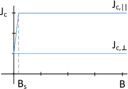
(a)

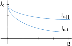
(b)

Figure 1: Using a magnetic field dependence for $J_{c\parallel}$ and $J_{c\perp}$ avoids indeterminations at ${\bf B}=0$. (a) Elliptic double critical-state model (CSM). (b) Anisotropic Kim model.

II.3 Sector minimization

Reduction of computing time is of essential importance for 3D calculations. We already studied the case of parallel minimization by sectors, where sectors are overlapping by one cell Pardo and Kapolka (2017a). In this article, we increase the overlapping of sectors in the following way. Now, the sectors are not overlapping to each other, and hence they share only the edge on the border, which are not solved (figure 2(a)). Then, we added other 2 sets of sectors, but the boundary in each set of sectors is shifted along the diagonal by 1/3 of the sector-diagonal size (figure 2(b,c)). The edge in the boundary in the first set is solved at least once in some of the other two sets. The additional sets increase the memory usage, which is still low, but they decrease the computing time. Sets of the sectors are minimized in series one after the other, but sectors within each set are solved in parallel to achieve high efficiency of parallel computing. Although computing all three sets of sectors in parallel could further enhance parallelization, we have found that solving each set sequentially reduces computing time. The process of solving all 3 sets subsequently is repeated until the maximum difference in any component of ${{\bf T}}$ between two iterations of the same set is below a certain tolerance. We use elongated cells, in order to improve the accuracy for a given number of cells, as detailed in appendix A.

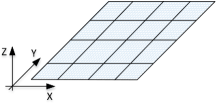
(a)

(b)

(c)

Figure 2: Using three sets of sectors speeds up the calculations. (a) Boundaries of the first set only. (b) First and second set. (c) All three sets.

III Results and discussion

As a result of the variational model, we calculated two geometries like an infinitesimally thin film (or simply, “thin film”) and a thin prism with finite thickness (or “thin prism”) [figure 3 (a),(b)]. The force-free effects are modelled with the anisotropic power-law in combination of either constant ${J_{c\perp}}$, ${J_{c\parallel}}$ or Kim model ${J_{c\perp}(B)}$, ${J_{c\parallel}(B)}$. We calculated as well the pure isotropic case of a thin film and thin prism for comparison. The calculations are performed with two values of the $n$-factor, 30 and 100, in order to have results close to the realistic values and analytical critical-state formulas, respectively.

III.1 Anisotropic force-free effects in films

In this section, we study square thin films of dimensions 12$\times$12 mm² and thickness 1 $\mu$m. We also take the common assumption of the thin film limit, which consists on averaging the electromagnetic properties over the sample thickness. For our method, this is achieved by taking only one cell along the sample thickness. We used a total number of degrees of freedom of 4200.

III.1.1 Power device situation

In this section, the magnetic applied field ${{\bf{B}}_{a}}$ has a sinusoidal waveform of 50 Hz and the same perpendicular, ${B_{a,z}}$, component for all angles ${\theta}$ with amplitude ${B_{a,z,m}=}$ 50 mT [figure 3(a)]. The angle ${\theta=0\degree}$ is completely perpendicular to the surface of the thin film. We calculated the cases with ${\theta=0\degree,45\degree,60\degree,80\degree}$. For this study, the perpendicular critical current density ${J_{c\perp}}$ is equal to ${3\cdot 10^{10}}$ A/m² and ${J_{c\parallel}}$ is 3 times higher. The dependence of ${J_{c}}$ on the magnetic field is on figure 1(a), where we choose ${B_{s}=}$ 1 mT. The $n$ factor of the anisotropic power law is equal 30, which is a realistic value for REBCO tapes in self-field.

The first case, with ${\theta=0\degree}$, is shown on figure 4. The penetration of the current density to the film strip is explained by colour maps of ${|{\bf J}|}$ normalized to ${J_{c\perp}}$, while the lines are current flux lines. The current density gradually penetrates to the sample after increasing the applied field [figure 4(a)], until it reaches almost saturated state at the peak of applied field [figure 4(b)]. During the decrease of the applied field, current starts penetrating again from the edges of the sample with opposite sign till the centre. The quasi remanent state, at ${B_{a}\approx}$0 mT, presents symmetric penetration of ${{\bf J}}$ along both ${x}$ and ${y}$ axis [figure 4(c)]. We show the first time step after remanence, ${{\bf B}=0}$, for comparison with the cases with ${\theta\neq 0\degree}$, where we use ${{\bf B}}$ of the previous time step in order to obtain ${J_{c\parallel}}$ [figure 4(a)].

The second case is for ${\theta=45\degree}$ and applied field amplitude ${B_{am}=}$70.7 mT (figure 5). The force-free effects appear during the increase of the applied field [figure 5(a)]. The current lines parallel to the ${x}$ axis are more aligned with the direction of the applied field. Therefore, ${J_{c\parallel}}$ becomes relevant, and hence current density at that direction is higher compared to the current density along the ${y}$ axis. The current penetration depth is smaller from top and bottom at the peak [figure 5(b)] compared to that from the sides. The penetration depth of ${J_{y}}$ from right and left is the same as for ${\theta=0\degree}$, because ${J_{y}}$ is still perpendicular to ${B_{a}}$. The quasi remanent state [figure 5(c)] with the applied field close to zero experiences the self-field as dominant component of the local magnetic field. Then, the self-field in the thin film approximation has only ${B_{z}}$ component, which is completely perpendicular to the surface and the current density. Therefore, only ${J_{c\perp}}$ is relevant and the maximum ${{\bf J}}$ in the sample is decreased back to that value.

The last two cases, ${\theta=60\degree}$ and ${80\degree}$, present similar behavior. The penetration of ${J_{x}}$ to the sample is even smaller during the increase of the applied field [figures 6(a), 7(a)], because of the higher angles ${\theta=60\degree,80\degree}$. The maximum ${J_{x}}$ component at the peak of the applied field [figures 6(b), 7(b)] is reaching 2.5 and 3 times of ${J_{c\perp}}$, which is the value of ${J_{c\parallel}}$. Again, at remanent state [figures 6(c), 7(c)] the maximum ${J_{x}}$ component is decreased back to values around ${J_{c\perp}}$ because of the self-field without any parallel component of the local magnetic field.

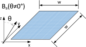
(a)

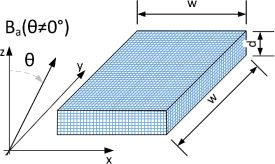
(b)

Figure 3: Sketches of the geometry with the variable angle ${\theta}$ of the applied magnetic field (a) thin strip (b) prism.

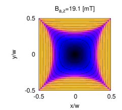
(a)

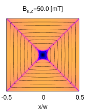
(b)

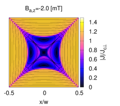
(c)

Figure 4: Penetration process of the critical-current density in the thin film with force-free anisotropic ${\bf E}({\bf J})$ relation. The applied magnetic field is sinusoidal with $\theta=0$ (perpendicular to the surface), ${B_{am}=}$50 mT, and ${f=}$50 Hz. (a) Initial curve. (b) Peak of the applied field. (c) Quasi-remanent state. The figure also shows the current flux lines.

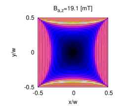
(a)

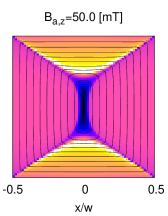
(b)

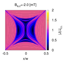
(c)

Figure 5: The same as figure 4 but for $\theta=45^{\rm o}$.

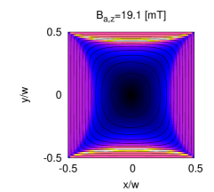
(a)

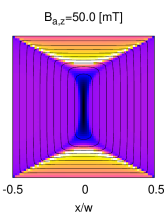
(b)

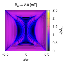
(c)

Figure 6: The same as figure 4 but for $\theta=60^{\rm o}$.

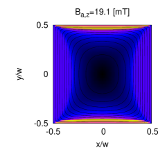
(a)

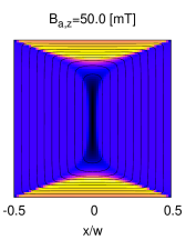
(b)

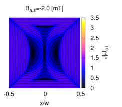
(c)

Figure 7: The same as figure 4 but for $\theta=80^{\rm o}$. For sufficiently large applied fields (a,b) there appear zones with $|{\bf J}|\approx J_{c\perp}$ and $|{\bf J}|\approx J_{c\parallel}$, while at the quasi-remanent state (c) $|{\bf J}|$ is limitted to $J_{c\perp}$.

The hysteresis loops for all angles ${\theta}$ of the applied field are on figure 8(a). The larger the applied-field angle, the higher the impact of ${J_{c\parallel}}$, and hence there exist places with the current density around ${J_{c\parallel}}$. The current density around ${J_{c\parallel}}$ creates higher magnetic moment in comparison to ${\theta=0\degree}$ where ${|{\bf J}|}$ is limited by ${J_{c\perp}}$. The self-field is dominant at the range of the applied field ${\pm}$5 mT, causing a mostly perpendicular local magnetic field, and hence $|{\bf J}|$ is again limited to $J_{c\perp}$. This is the reason why the magnetization is decreasing back to the same value as in the case of ${\theta=0\degree}$. We calculated the same situation with isotropic power law. The results of the isotropic case are the same for each angle ${\theta}$ because the perpendicular applied field is the same as for ${\theta=0\degree}$ [see magnetization loops in figure 8(b)]. Consistently, these magnetization loops also agree with the anisotropic case with ${\theta=0\degree}$, since $J_{c}=J_{c\perp}$ for the whole loop [figure 8(a)].

III.1.2 Magnet situation

The next calculation assumes the same parameters and geometry as the previous cases. The difference is in the $n$-factor, with value 100, triangular waveform of the applied field of 1 mHz frequency and amplitude ${B_{a,z,m}=}$ 150 mT. This magnetization is qualitatively similar to magnet charge and discharge. The angles of applied field are the same ${\theta=0\degree,45\degree,60\degree,80\degree}$. The high $n$-factor reduces the current density to values equal or below ${J_{c\perp}}$ or ${J_{c\parallel}}$. Another reason for reduction of current density is the very low frequency of the applied field, which allows higher flux relaxation. The constant ramp rate causes that the magnetization loops are flat after the sample is fully saturated [figure 9(b)]. The case of ${\theta=0\degree}$ induces only current density perpendicular to the applied field, and hence magnetization loop is horizontal at the remanent state. Again, we see a minimum at remanence for higher $\theta$.

The last thin film example assumes anisotropic power law with two critical current densities, which depends on the magnetic field according Kim model ${J_{c\parallel}(B)}$, ${J_{c\perp}(B)}$. The dependence is on figure 1(b). The magnetic field ${{\bf B}}$ is calculated in the same time step ${{\bf B}(t)}$ as the functional is minimized, and hence now the remanent state is straightforwardly for ${{\bf B}=0}$ as it is shown on figure figure 10(b). The ${B_{a,z}}$ component of the maximum applied field is 300 mT and it is the same for all angles ${\theta}$. The magnetization of the sample [figure 10(a)] is higher close to the remanent state, since the applied field is close to zero and the self-field only slightly decreases the critical current density. With increasing the applied field from the zero-field-cool situation, the sample becomes fully saturated already at 40 mT. With further increase of the applied field, the Kim dependence causes a decrease in $J_{c\parallel}$,$J_{c\perp}$ and $|{\bf J}|$, decreasing the magnitude of the magnetization. The highest magnetization is at the applied field with ${\theta=80\degree}$, in spite of ${|{\bf B}_{a}|}$ being the largest and hence reducing the most ${J_{c\perp}}$ and ${J_{c\parallel}}$. The cause is that there still exist areas with current density around ${J_{c\parallel}}$. At the remanent state, we can see again reduction of magnetization to the level of ${\theta=0\degree}$ [figure 10(b)].

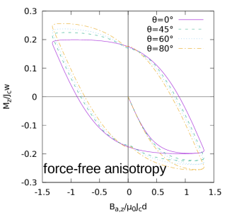
(a)

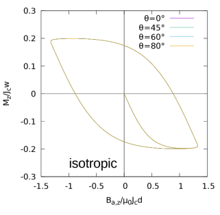
(b)

Figure 8: Force free anisotropy increases the magnetization at the peak of the applied field. Case for thin film with $n$ value 30, sinusoidal applied magnetic field ${B_{a,z}=}$50.0 mT and ${f=}$50 Hz. (a) Force-free anisotropic power law. (b) Isotropic power law.

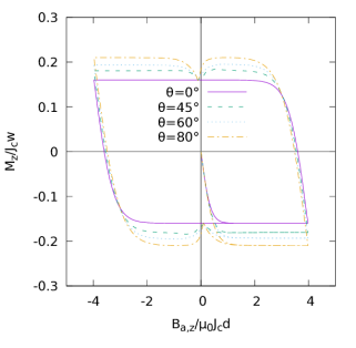
Figure 9: For a triangular waveform of the applied field, the minimum at remanence of the hysteresis loops is very pronounced. Calculations for the force-free anisotropic power law of $n=$100 and triangular applied magnetic field with $B_{a,m}=$ 150.0 mT, ${B_{a,zm}=}$50 mT and ${f=}$1 mHz.

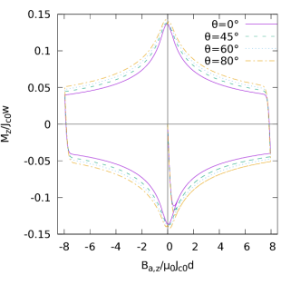
(a)

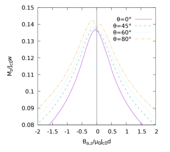
(b)

Figure 10: (a) With a Kim-like dependence of $J_{c\parallel}$ and $J_{c\perp}$, the area of the magnetization loop increases with $\theta$ due to force-free effects. (b) This zoom at low applied field shows the minimum of the remanence. The parameters are $n=100$ and triangular applied magnetic field with $B_{az,m}=$300 mT and $f=$1 mHz.

III.2 Anisotropic force-free effects in prisms

III.2.1 Current density in prisms.

In the following, we analyze the force-free effects in a prisms. We model the prisms with the same dimensions as thin film ${12\times 12}$ mm but thickness 1 mm. The mesh of the sample is created by elongated cells, which we explain in A. The total number of cells is ${31\times 31\times 15}$, which corresponds to around 43000 degrees of freedom. The frequency of the applied filed is 50 Hz and the amplitude of the $z$ component of ${\bf B}_{a}$ is 50 mT for all angles ${\theta=0,\degree 45\degree,60\degree,80\degree}$; and hence the total amplitude is $B_{a,m}=$50, 70.7, 100 and 287.9 mT, respectively. The critical current densities are chosen so that the sheet critical current density $K_{c}\equiv{J_{c}d}$ is the same as for the thin film, being ${d}$ the sample thickness. Further values are ${J_{c\perp}=3\cdot 10^{7}}$ A/mm², ${J_{c\parallel}=3J_{c\perp}}$ and ${n}$=30.

The force-free effects are modelled with the anisotropic power law and the sharp dependence of $J_{c\parallel}$ with the magnetic field of figure 1(a). Then, the functional is minimized with the magnetic field from the previous time step like in the case of thin film.

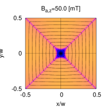
(a)

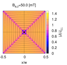
(b)

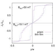
(c)

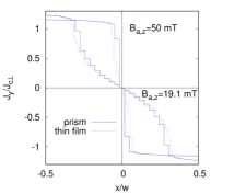
(d)

Figure 11: For low angles of the applied field, the thickness-averaged current density in a prim agrees with the thin film. Thickness-average current density and flux lines for a thin film (a) and prism (b). Plots (c) and (d) show the current density at the $x=0$ and $y=0$ lines, respectively. The parameters are $\theta=0$, $B_{az,m}$=50 mT and $f=$50 Hz.

The first case is with applied field ${\theta}$=0${\degree}$. We calculated the average current density over thickness. The penetration of the average current density into the prism at the peak of applied field is on figure 11, where we add the case of thin film for comparison. There is a small difference in penetration depth of the current density, which can be explained by different number of elements in the $x$ and $y$ directions. The result of prism looks coarser, but we solved 10 times higher number of degrees of freedom compared to the thin film, since the prism is a 3D object. The smaller penetration in thin film is more visible in the profiles over the $x$ and $y$ directions on the sample center [figure 11(c),(d)], also for a lower applied field. For these planes, $J_{z}$ vanishes due to symmetry, although $J_{z}\neq 0$ at other regions Pardo and Kapolka (2017b).

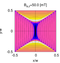
(a)

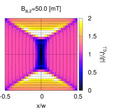
(b)

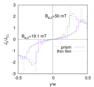
(c)

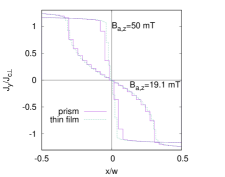
(d)

Figure 12: The same as figure 11 but for $\theta=45^{\rm o}$. The transverse component of the applied field amplitude of $B_{az,m}$=50 mT requires a total amplitude of $B_{am}=$70.7 mT.

The second case of prism is ${\theta=45\degree}$. The penetration depth of the average current density in the prism [figure 12(b)] agrees with the thin film case [figure 12(a)]. The agreement is as well in the lines of ${x=0}$ and ${y=0}$ [figure 12(c),(d)]. The ${J_{y}}$ component of the current density is around ${J_{c\perp}}$ [figure 12(d)], but ${J_{x}}$ is 2 times higher. The reason of the higher magnitude of $J_{x}$ is that the applied field has a component in the $x$ direction, causing force-free effects. This also causes that $J_{x}$ at the penetration front reaches $J_{c\parallel}$ in the thin film, since $B_{z}$ there vanishes (figure 12). The penetration depth in the prism is smaller, because of the thicker cells.

The last two cases with ${\theta=60\degree,80\degree}$ are similar to the appropriate cases of thin film, although with certain differences. For the angle ${\theta=60\degree}$ there is lower penetration depth from the right and left sides [figure 13(b)] than the thin film [figure 13(a)]. The angle ${\theta=80\degree}$ has even lower penetration depth from these sides [figure 14(b)] compared to thin film [figure 14(a)]. The current profiles along the $x$ and $y$ directions show the same behaviour of lower current penetration [figure 13(c),(d), 14(c),(d)]. The cause of lower penetration depth along both $x$ and $y$ directions is due to the prism finite thickness. Since ${\theta\neq 0\degree}$, there is a significant ${J_{z}}$ component of the current density, which is around ${J_{c\perp}}$[figure 16(c) ${\theta=80\degree}$].

Finally, we compare the 3D current paths in the prism at the peak of the applied field for the anisotropic case and two applied field angles ${\theta=0\degree}$ and ${80\degree}$. For the first angle, the sample is fully saturated as seeing the mid planes perpendicular to the ${x}$ and ${y}$ axis [figure 15(a),(b)] and hence $J_{z}$ almost vanishes [figure 15(c)]. For the second angle $(\theta=80\degree)$, the ${J_{y}}$ component of the current density is also saturated in most of the volume [figure 16(b)]. Now, the border between positive and negative ${J_{y}}$ component follows roughly the direction of the applied magnetic field. The ${J_{x}}$ component is not saturated in the sample [figure 16(a)] and the highest penetration depth is at the centre of the prism. Since the current loops are almost perpendicular to the angle of the applied field, there exists a substantial $J_{z}$ component [figure 16(c)].

III.2.2 Magnetization loops in prisms.

We calculated the hysteresis loops for all previous cases (figure 17). In order to explain all effects, we also analyzed the same situation with isotropic power law (figure 18). The ${M_{z}}$ component of the magnetization is lower for higher applied magnetic field angle ${\theta}$ [figure 18(b)]. This is because the path of the screening current loops tilts away from the $xy$ plane. The ${M_{x}}$ component is zero for ${\theta=0\degree}$ [figure 18(a)], since the current path is only in the $xy$ plane. This also causes and increase of the $M_{x}$ component with increasing $\theta$. This geometry effect can be reduced by decreasing the prism thickness. Consistently, $M_{x}$ vanishes at $\theta=0$ because the current loops are mainly in the $xy$ plane and the remaining bending in the $z$ direction is symmetric (see figure 5 of Pardo and Kapolka (2017b)).

The hysteresis loops with anisotropic ${{\bf E}({\bf J})}$ relation have more effects. On one hand, increasing the angle $\theta$ enlarges the region with $|{\bf J}|\approx J_{c\parallel}$, increasing also $M_{z}$. On the other hand, by increasing $\theta$, the tilt increases, reducing $M_{z}$. The result is an increase in $M_{z}$ with $\theta$ but for $\theta=80^{\rm o}$ this increase is smaller than for the thin film [figure 17(b)]. The magnetization in the ${x}$ direction [figure 17(a)] shows mostly the same behavior as isotropic case. The difference is only in a peak of the magnetization around the zero applied field. This peak of the magnetization appears for both components, ${M_{x}}$ and ${M_{z}}$. The reason of this peak is the following. For very small magnetic fields, the self-field dominates. Close to the top (highest $z$) and bottom (lowest $z$) of the sample, the self-field is parallel to the surface. Then, part of the sample experiences a local magnetic field parallel to the current density, increasing $J_{c}$ towards $J_{c\parallel}$. For applied fields much larger than the self-field, the magnetic field follows the direction of the applied field. This applied field is not perfectly parallel to the surface, causing a lower $J_{c}$.

Another calculation with isotropic ${\bf E}({\bf J})$ relation shows the geometry effects due to different thickness of the prism ($d=$1,0.6,0.5,0.1) while keeping a constant sheet current density. First we check that for only perpendicular applied field, the prism results approach to the thin film by reducing the thickness. Figure 19 shows that the normalized $z$ component $M_{z}/J_{c}w$ is roughly the same for all thicknesses $d$. This figure also tells us that the magnetic moment $m_{z}$ almost does not depend on $d$, since $M_{z}/J_{c}w=m_{z}/J_{c}dw^{3}$ and we keep both $J_{c}d$ and $w$ constant. For a magnetic field angle $\theta$ of $80^{\rm o}$, $M_{z}$ increases with decreasing the sample thickness, since the screening current is forced to flow closer to the $xy$ plane [figure 20(b)]. However, the other normalized component, $M_{x}/J_{c}d$, increases with the thickness $d$, due to the increase of the area of the projection of the current loops in the $yz$ plane.

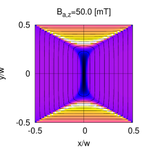
(a)

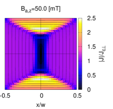
(b)

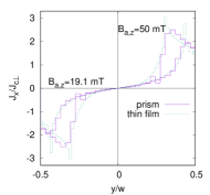
(c)

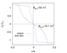
(d)

Figure 13: The same as figure 11 but for $\theta=60^{\rm o}$ ($B_{az,m}$=50 mT and $B_{am}=$100 mT). A slightly lower critical-current penetration can be observed from the prism (b,d) compared to the film (a,c).

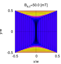
(a)

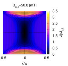
(b)

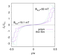
(c)

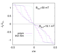
(d)

Figure 14: The same as figure 11 but for $\theta=80^{\rm o}$ ($B_{az,m}$=50 mT and $B_{am}=$287.9 mT). The prism (b,d) presents a substantially lower penetration of the critical-current density than the film (a,c).

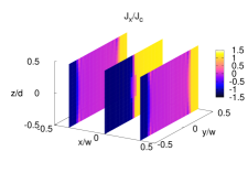
(a)

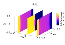
(b)

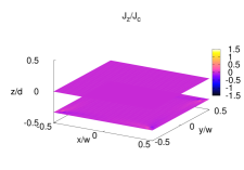
(c)

Figure 15: Current density in a prism with force-free anisotropy at the peak of the applied field and $w=$12 mm, $d$=1 mm, $\theta=0^{\rm o}$, and $B_{az,m}=$50 mT. The current density components are: (a) ${J_{x}}$ (b) ${J_{y}}$ (c) ${J_{z}}$. Note that the plotted planes in (b) are not the same as (a,c).

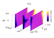
(a)

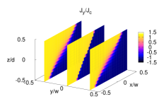
(b)

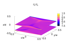
(c)

Figure 16: The same as figure 15 but for $\theta=80^{\rm o}$ ($B_{am}=287.9$ mT).

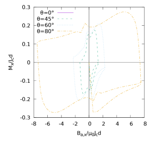
(a)

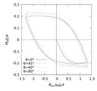
(b)

Figure 17: The influence of the applied field angle to the magnetization loops in a prism is somewhat different than that of a thin film with the same sheet critical current density $J_{c}d$. Case of anisotropic ${{\bf E}({\bf J})}$ relation and constant ${J_{c\parallel}}$, ${J_{c\perp}}$, $n=$ 30, sinusoidal applied magnetic field with ${B_{a,z}=}$50.0 mT and ${f=}$50 Hz. (a) The $x$ component of the magnetization ${M_{x}}$ component. (b) ${M_{z}}$.

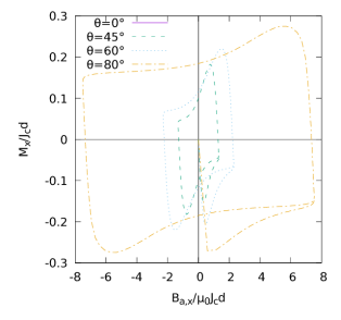
(a)

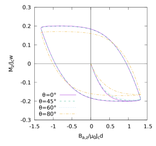
(b)

Figure 18: The same as figure 17 but for isotropic ${\bf E}({\bf J})$. Several differences appear from the anisotropic case, such as the peaks close to the remanence in figure 17.

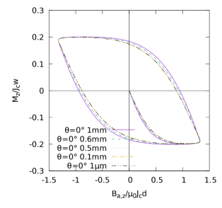
Figure 19: For isotropic ${\bf E}({\bf J})$ in prisms and $\theta=0$, the normalized magnetization converges to the thin film situation. The properties are $n=$30, sinusoidal applied magnetic field ${B_{a,z}=}$50.0 mT and ${f=}$50 Hz.

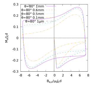
(a)

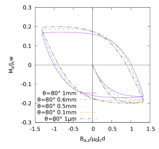
(b)

Figure 20: Hysteresis loops of prisms with several thicknesses $d$ and the same width $w$ with isotropic ${{\bf E}({\bf J})}$ relation and constant $J_{c}$, $n=$30, and sinusoidal applied magnetic field with ${B_{a,z}=}$50.0 mT and ${f=}$50 Hz. (a) ${M_{x}}$ component. (b) ${M_{z}}$ component

IV Conclusions

This article systematically studied the anisotropic force-free effects in superconducting thin films and prisms under uniform applied magnetic field making on angle $\theta$ with the surface. In order to better understand all effects, we performed modelling with isotropic and anisotropic ${{\bf E}({\bf J})}$ relation due to force-free effects.

For this purpose, we use the MEMEP 3D numerical method Pardo and Kapolka (2017a). We further developed the model in order to enable elongated cells, to reduce the total number of elements or enable to model relatively long or thin structures without further increasing the total number of elements. In particular, we studied the elliptical double critical state model with a continuous ${\bf E}({\bf J})$ relationBadía-Majós and López (2012).

In the thin film force-free model, we calculated the gradual penetration of the current density. We found at the remanent state that ${J}$ decreases to $J_{c\perp}$ and the magnetization increases with the angle $\theta$. The magnetization of the isotropic film is the same for all applied field angles, when comparing for the same perpendicular component of the applied magnetic field and its amplitude. The anisotropic model, both with and without $J_{c}(B)$ dependence, shows a minimum of the magnetization at the remanent state for $\theta\neq 0$. The cause is the absence of any parallel component of the local magnetic field to the current density, avoiding $J_{c}$ enhancement due to force-free effects. In superconducting prisms, we observed 3D current paths. The average current density over thickness shows good agreement with thin film sample. However, for high applied magnetic field angles there appear small differences. The $M_{x}$ component is increasing with the angle $\theta$, because of the significant increase of $J_{z}$. The $M_{z}$ slightly decreases due to the tilt in the screening currents. The magnetization loops show a peak after the remanent state due to the influence of the parallel component of the self-field, increasing $J_{c}$ up to $J_{\parallel}$ at part of the sample. This effect is not present for the thin film approximation because the parallel component of the self-field is neglected. Calculations for several prism thicknesses down to 100 $\mu$m support the validity of the results.

We expect that the thin film geometry may not be a good approximation for study force-free effects in magnetization measurements. This study confirmed that the MEMEP 3D method is suitable for any ${{\bf E}({\bf J})}$ relation and it can be solved with a relatively high number of degrees of freedom and relatively thin samples in 3D space. Further work could be to investigate different shapes of the sample and speed up the calculation, maybe by multi-pole expansion.

Appendix A Elongated cells

The elongated cells are cells with different geometry ratio than square (for 2D) or cubic (for 3D) . These cells allow to model geometries such as long thin film, or thin/thick bulk. The elongated cells enable to reduce the total number of elements, and hence reduce the computing time. A key issue is the calculation of the interaction matrix between elemental surfaces (or “surfaces”). The interaction matrix between surfaces ${i}$ and ${j}$ of type ${s\in\{x,y,z\}}$ is generally Pardo and Kapolka (2017a)

$$a_{sij}=\frac{\mu_{0}}{4\pi V_{si}V_{sj}}\int_{V_{si}}{{\rm d}^{3}{\bf r}}\int_{V_{sj}}{{\rm d}^{3}{\bf r}}^{\prime}\frac{h_{si}({\bf r})h_{sj}({\bf r}^{\prime})}{|{\bf r}-{\bf r}^{\prime}|},$$ (16)

with

$$V_{si}\equiv\int_{V}{{\rm d}^{3}{\bf r}}h_{si}({\bf r}).$$ (17)

The first-order interpolation functions ${h_{si}({\bf r})}$ are defined as in figure 21(b) for coordinate ${r_{s}=r_{x}}$, vanishing outside the two neighboring cells in the ${r_{s}}$ direction.

In the case of square or cubic cells or square sub-elements, the self-interaction term ${a_{sii}}$ can be calculated by the approximated analytical formula

$$a_{sii}\approx\frac{\mu_{0}}{4\pi V_{si}{{}^{2}}}\int_{V_{si}}{{\rm d}^{3}{\bf r}}\int_{V_{si}}{{\rm d}^{3}{\bf r}}^{\prime}\frac{1}{|{\bf r}-{\bf r}^{\prime}|}.$$ (18)

The integral $\int_{V_{si}}{\rm d}^{3}{\bf r}\int_{V_{sj}}{\rm d}^{3}{\bf r}^{\prime}(1/|{\bf r}-{\bf r}^{\prime}|)$ on a rectangular prism is a lengthy analytical formula. For a cube and a square surface, the expression can be greatly simplified as

$$a_{sii}\approx\frac{\mu_{0}}{4\pi L_{si}}\left\{\frac{1+\sqrt{2}-2\sqrt{3}}{5}-\frac{\pi}{3}+\ln\left[\left(1+\sqrt{2}\right)\left(2+\sqrt{3}\right)\right]\right\}$$ (19)

for a cube of side $L_{si}$ Ciftja (2011) and

$$a_{sii}\approx\frac{\mu_{0}}{\pi L_{si}}\left\{\frac{1-\sqrt{2}}{3}+\ln\left(1+\sqrt{2}\right)\right\}$$ (20)

for a thin prism Ciftja (2010) with thickness $d$ much smaller than its side $L_{si}$. For equation (18) we assumed that the current density is uniform in the volume of influence, defined as the volume between surface ${i}$ of type ${s}$ and the centre of the neighbouring cells in the ${s}$ direction (see figure 21(a) for ${s=x}$). The average vector potential ${a_{sij}}$ is calculated by approximation everywhere else, ${i\neq j}$

$$a_{sij}\approx\frac{\mu_{0}}{4\pi|r_{si}-r_{sj}|},$$ (21)

where ${r_{si}}$ is the centre of surface ${i}$ of type ${s}$.

In the case of elongated cells, the interaction matrix of the vector potential, ${a_{sij}}$ needs to be calculated numerically. The numerical calculation splits the surrounded area of two surfaces into small square sub-elements (figure 21(a)). The average vector potential of the two surfaces is integrated over all sub-elements, which contain surfaces again. The sub-elements are calculated in the same way as square cells, but sub-elements are multiplied by the linear interpolations functions ${h_{si}({\bf r}),h_{sj}({\bf r})}$ at the centre of the sub-element surfaces with indexes ${l,m}$, being ${{\bf r}_{sl}}$ and ${{\bf r}_{sm}}$. Elongated cells contain as many sub-elements in order to reach as square as possible shape. In general, the average vector potential generated by sub-element $l$ on sub-element $m$ is

$$a_{sijlm}=\frac{\mu_{0}}{4\pi V_{sl}V_{sm}}\int_{V_{sl}}{{\rm d}^{3}{\bf r}}\int_{V_{sm}}{{\rm d}^{3}{\bf r}}^{\prime}\frac{h_{si}({\bf r}_{sl})h_{sj}({\bf r}_{sm})}{|{\bf r}-{\bf r}^{\prime}|},$$ (22)

where $V_{sl}$ and $V_{sm}$ are the volume of influence of the sub-elements, as defined in figure 21(a). For $l\neq m$, we approximate the integral above by

$$a_{sijlm}\approx\frac{\mu_{0}h_{si}({\bf r}_{sl})h_{sj}({\bf r}_{sm})}{4\pi|{\bf r}_{sl}-{\bf r}_{sm}|},$$ (23)

where ${V_{sl}}$ is the volume of the influence of the sub-elements, defined in figure 21(a). When $l$ corresponds to the sub-element $m$ both in position and size, we use the approximated formula for uniform current density in the sub-element

$$a_{sijll} \approx \frac{\mu_{0}h_{si}({\bf r}_{sl})h_{sj}({\bf r}_{sl})}{4\pi V_{sl}^{2}}\int_{V_{sl}}{{\rm d}^{3}{\bf r}}\int_{V_{sl}}{{\rm d}^{3}{\bf r}}^{\prime}\frac{1}{|{\bf r}-{\bf r}^{\prime}|}.$$ (24)

Following the same steps as for equation (18), $a_{sijll}$ becomes

$$a_{sijll} \approx \frac{\mu_{0}h_{si}({\bf r}_{sl})h_{sj}({\bf r}_{sl})}{4\pi L_{sl}}$$ (25)

$$\cdot\left\{\frac{1+\sqrt{2}-2\sqrt{3}}{5}-\frac{\pi}{3}+\ln\left[\left(1+\sqrt{2}\right)\left(2+\sqrt{3}\right)\right]\right\}$$

for a cube of side $L_{sl}$ and

$$a_{sijll}\approx\frac{\mu_{0}h_{si}({\bf r}_{sl})h_{sj}({\bf r}_{sl})}{\pi L_{sl}}\left\{\frac{1-\sqrt{2}}{3}+\ln\left(1+\sqrt{2}\right)\right\}$$ (26)

for a thin prism of side $L_{sl}$.

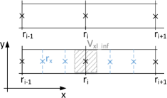
(a)

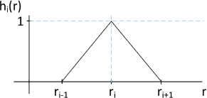
(b)

Figure 21: (a) Dividing elongated cells into sub-elements enables to compute accurate interaction matrix elements. Solid lines: original elongated mesh. Dash lines: sub-elements mesh. (b) Interpolation ${h_{i}(r)}$ function.

References

- Larbalestier et al. (2014) D. C. Larbalestier, J.Jiang, U. P. Trociewitz, F. Kametami, C. Scheuerlein, M. Dalban-Canassy, M. Matras, P. Chen, N. C. craig, P. J. Lee, and E. E. Hellstrom, “Isotropic round-wire multifilament cuprate superconductor for generation of magnetic fields above 30 T,” Nature Materials 13, 375–381 (2014).
- Kim et al. (2017) K. Kim, K. R. Bhattarai, J. Y. Jang, Y. J. Hwang, K. Kim, S. Yoon, S. Lee, and S. Hahn, “Design and performance estimation of a 35 T 40 mm no-insulation all-REBCO user magnet,” Supercond. Sci. Technol. 30 (2017).
- Park et al. (2018) D. Park, J. Bascunan, P. Michael, J. Lee, S. Hahn, and Y. Iwasa, “Construction and test results of coils 2 and 3 of a 3-nested-coil 800-MHz REBCO insert for the MIT 1.3-GHz LTS/HTS NMR Magnet,” IEEE Trans. Appl. Supercond. 28 (2018).
- Liu and Li (2016) J. Liu and Y. Li, “High-Field Insert With Bi- and Y-Based Tapes for 25-T All-Superconducting Magnet,” IEEE Trans. Appl. Supercond. 26 (2016).
- Masson et al. (2007) P. J. Masson, M. Breschi, T. Pascal, and C. Luongo, “Design of HTS axial flux motor for aircraft propulsion,” IEEE Trans. Appl. Supercond. 17 (2007).
- Masson et al. (2013) P. J. Masson, K. Ratelle, P. A. Delobel, A. Lipardi, and C. Lorin, “Development of a 3D sizing model for all-superconducting machines for turbo-electric aircraft propulsion,” IEEE Trans. Appl. Supercond. 23, 3600805 (2013).
- Yanamoto et al. (2017) T. Yanamoto, M. Izumi, K. Umemoto, T. Oryu, Y. Murase, and M. Kawamura, “Load test of 3-MW HTS motor for ship propulsion,” IEEE Trans. Appl. Supercond. 27 (2017).
- Gamble et al. (2011) B. Gamble, G. Snitchler, and T. MacDonald, “Full power test of a 36.5 MW HTS propulsion motor,” IEEE Trans. Appl. Supercond. 21, 1083–1088 (2011).
- Jeong et al. (2017) JS. Jeong, DK. An, JP. Hong, HJ. Kim, and YS. Jo, “Design of a 10-MW-Class HTS homopolar generator for wind turbines,” IEEE Trans. Appl. Supercond. 27 (2017).
- Abrahamsen et al. (2010) A.B. Abrahamsen, N. Mijatovic, E. Seiler, T. Zirngibl, C. Træholt, P.B. Nørgård, N.F. Pedersen, N.H. Andersen, and J. Østergaard, “Superconducting wind turbine generators,” Supercond. Sci. Technol. 23, 034019 (2010).
- (11) SUPRAPOWER-EU project. Superconducting light generator for large offshore wind turbines. http://www.suprapower-fp7.eu/.
- Volkov et al. (2012) E. Volkov, V. Vysotsky, and V. Firsov, “First russian long length HTS power cable,” Physica C-Superc. and its apl. 482, 87–91 (2012).
- Yagi et al. (2015) M. Yagi, J. Liu, S. Mukoyama, T. Mitsuhashi, J. Teng, N. Hayakawa, W. Wang, A. Ishiyama, N. Amemiya, T. Hasegawa, T. Saitoh, O. Maruyama, and T. Ohkuma, “Experimental results of 275-kV 3-kA REBCO HTS power cable,” IEEE Trans. Appl. Supercond. 25 (2015).
- Hellmann et al. (2017) S. Hellmann, M. Abplanalp, L. Hofstetter, and M. Noe, “Manufacturing of a 1-MVA-Class superconducting fault current limiting transformer with recovery-under-load capabilities,” IEEE Trans. Appl. Supercond. 27 (2017).
- Glasson et al. (2017) N. Glasson, M. Staines, N. Allpress, M. Pannu, J. Tanchon, E. Pardo, R. Badcock, and R. Buckley, “Test results and conclusions from a 1 MVA superconducting transformer featuring 2G HTS roebel cable,” IEEE Trans. Appl. Supercond. 27 (2017).
- Schwenterly et al. (1999) S. Schwenterly, B. McConnell, J. Demko, A. Fadnek, J. Hsu, F. List, M. Walker, D. Hazelton, F. Murray, J. Rice, C. Trautwein, X. Shi, R. Farrell, J. Bascunan, R. Hintz, S. Mehta, N. Aversa, J. Ebert, B. Bednar, D. Neder, A. McIlheran, P. Michel, J. Nemec, E. Pleva, A. Swenton, N. Swets, R. Longsworth, RC. Longsworth, R. Johnson, R. Jones, J. Nelson, R. Degeneff, and S. Salon, “Performance of a 1-MVA HTS demonstration transformer,” IEEE Trans. Appl. Supercond. 9, 680–684 (1999).
- Mehta (2011) S. Mehta, “US effort on HTS power transformers,” Physica C 471, 1364–1366 (2011).
- Pascal et al. (2017) T. Pascal, A. Badel, G. Auran, and GS. Pereira, “Superconducting fault current limiter for ship grid simulation and demonstration,” IEEE Trans. Appl. Supercond. 27 (2017).
- Xin et al. (2013) Y. Xin, W. Gong, Y. Sun, J. Cui, H. Hong, X. Niu, H. Wang, L. Wang, Q. Li, J. Zhang, Z. Wei, L. Liu, H. Yang, and X. Zhu, “Factory and field tests of a 220 kV/300 MVA statured iron-core superconducting fault current limiter,” IEEE Trans. Appl. Supercond. 23 (2013).
- Morandi (2013) A. Morandi, “State of the art of superconducting fault current limiters and their application to the electric power system,” Physica C 484, 242–247 (2013).
- Šouc et al. (2012) J. Šouc, F. Gömöry, and M. Vojenčiak, “Coated conductor arrangement for reduced AC losses in a resistive-type superconducting fault current limiter,” Supercond. Sci. Technol. 25, 014005 (2012).
- Kozak et al. (2016) J. Kozak, M. Majka, T. Blazejczyk, and P. Berowski, “Tests of the 15-kV class coreless superconducting fault current limiter,” Supercond. Sci. Technol. 26 (2016).
- Durrell et al. (2003) J.H. Durrell, S.H. Mennema, C. Jooss, G. Gibson, Z. H. Barber, H.W. Zandbergen, and J.E. Evetts, “Flux line lattice structure and behavior in antiphase boundary free vicinal YBa2Cu3O7-δ thin films,” J. Appl. Phys. 93, 9869–9874 (2003).
- Lao et al. (2017) M. Lao, J. Hecher, M. Sieger, P. Pahlke, M. Bauer R. Huhne, and M. Eisterer, “Planar current anisotropy and field dependence of Jc in coated conductors assessed by scanning hall probe microscopy,” Supercond. Sci. Technol. 30, 9 (2017).
- Blatter et al. (1994) G. Blatter, M. V. Feigelman, V. B. Geshkenbein, A. I. Larkin, and V. M. Vinokur, “Vortices in high-temperature superconductors,” Rev. Mod. Phys. 66, 1125 (1994).
- Vlasko-Vlasov et al. (2015) V. Vlasko-Vlasov, A. Koshelev, A. Glatz, C. Phillips, U. Welp, and K. Kwok, “Flux cutting in high-Tc superconductors,” Phys. Rev. B (2015).
- Clem (1982) J.R. Clem, “Flux-line-cutting losses in type-II superconductors,” Phys. Rev. B 26, 2463 (1982).
- Clem et al. (2011) J.R. Clem, M. Weigand, J. H. Durrell, and A. M. Campbell, “Theory and experiment testing flux-line cutting physics,” Supercond. Sci. Technol. 24, 062002 (2011).
- Clem and Perez-Gonzalez (1984) J.R. Clem and A. Perez-Gonzalez, “Flux-line-cutting and flux-pinning losses in type-II superconductors in rotating magnetic fields,” Phys. Rev. B 30, 5041 (1984).
- Brandt and Mikitik (2007) E. H. Brandt and G. P. Mikitik, “Unusual critical states in type-II superconductors,” Phys. Rev. B 76 (2007).
- Romero-Salazar and Pérez-Rodríguez (2003) C. Romero-Salazar and F. Pérez-Rodríguez, “Elliptic flux-line-cutting critical-state model,” Appl. Phys. Lett. 83, 5256 (2003).
- Chepikov et al. (2017) V. Chepikov, N. Mineev, P. Degtyarenko, S. Lee, V. Petrykin, A. Ovcharov, A. Vasiliev, A. Kaul, V. Amelichev, A. Kamenev, A. Molodyk, and S. Samoilenkov, “Introduction of BaSnO3 and BaZrO3 artificial pinning centres into 2G HTS wires based on PLD GdBCO films. Phase I of the industrial RD programme at SuperOx,” Supercond. Sci. Technol. 30 (2017).
- Iijima et al. (2015) Y. Iijima, Y. Adachi, S. Fujita, M. Igarashi, K. Kakimoto, M. Ohsugi, N. Nakamura, S. Hanyu, R. Kikutake, M. Daibo, M. Nagata, F. Tateno, and M. Itoh, “Development for mass production of homogeneous RE123 coated conductors by hot-wall PLD process on IBAD template technique,” IEEE Trans. Appl. Supercond. 25 (2015).
- Lee et al. (2014) J. Lee, B. Mean, T. Kim, Y. Kim, K. Cheon, T. Kim, D. Park, D. Song, H. Kim, W. Chung, H. Lee, and S. Moon, “Vision inspection methods for uniformity enhancement in long-length 2g hts wire production,” IEEE Trans. Appl. Supercond. 24 (2014).
- Rossi et al. (2016) L. Rossi, X. Hu, F. Kametani, D. Abraimov, A. Polyanskii, J. Jaroszynski, and DC. Larbalestier, “Sample and length-dependent variability of 77 and 4.2 K properties in nominally identical RE123 coated conductors,” Supercond. Sci. Technol. 29 (2016).
- Xu et al. (2017) A. Xu, Y. Zhang, M. Gharahcheshmeh, L. Delgado, N. Khatri, Y. Liu, E. Galstyan, and V. Selvamanickam, “Relevant pinning for ab-plane J(c) enhancement of MOCVD REBCO coated conductors,” IEEE Trans. Appl. Supercond. 27 (2017).
- Lin et al. (2017) JX. Lin, XM. Liu, CW. Cui, CY. Bai, YM. Lu, F. Fan, YQ. Guo, ZY. Liu, and CB. Cai, “A review of thickness-induced evolutions of microstructure and superconducting performance of REBa2Cu3O7-delta coated conductor,” Advances in Manufacturing. 5, 165–176 (2017).
- Miura et al. (2017) S. Miura, Y. Tsuchiya, Y. Yoshida, Y. Ichino, S. Awaji, K. Matsumoto, A. Ibi, and T. Izumi, “Strong flux pinning at 4.2 K in SmBa2Cu3Oy coated conductors with BaHfO3 nanorods controlled by low growth temperature,” Supercond. Sci. Technol. 30 (2017).
- Ayai et al. (2008) N. Ayai, S. Kobayashi, M. Kikuchi, T. Ishida, J. Fujikami, K. Yamazaki, S. Yamade, K. Tatamidani, K. Hayashi, K. Sato, H. Kitaguchi, H. Kumakura, K. Osamura, J. Shimoyama, H. Kamijyo, and Y. Fukumoto, “Progress in performance of DI-BSCCO family,” Physica C-Superc. and its apl. 468, 1747–1752 (2008).
- Goyal et al. (1997) A. Goyal, DP. Norton, DM. Kroeger, DK. Christen, M. Paranthaman, ED. Specht, JD. Budai, Q. He, B. Saffian, FA. List, DF. Lee, E. Hatfield, PM. Martin, CE. Klabunde, J. Mathis, and C. Park, “Conductors with controlled grain boundaries: An approach to the next generation, high temperature superconducting wire,” J. Mar. Res. 12, 2924–2940 (1997).
- Pallecchi et al. (2015) I. Pallecchi, M. Eisterer A. Malagoli, and M. Putti, “Application potential of Fe-based superconductors,” Supercond. Sci. Technol. 28 (2015).
- Yi et al. (2017) W. Yi, Q. Wu, and LL. Sun, “Superconductivities of pressurized iron pnictide superconductors,” Acta Physica Sinica. 66 (2017).
- Ma et al. (2017) YH. Ma, QC. Ji, KK. Hu, B. Gao, W. Li, G. Mu, and XM. Xie, “Strong anisotropy effect in an iron-based superconductor CaFe0: 882Co0: 118AsF,” Supercond. Sci. Technol. 30 (2017).
- Hecher et al. (2018) J. Hecher, S. Ishida, D. Song, H. Ogino, A. Iyo, H. Eisaki, M. Nakajima, D. Kagerbauer, and M. Eisterer, “Direct observation of in-plane anisotropy of the superconducting critical current density in Ba(Fe1-xCox)(2)As-2 crystals,” Phys. Rev. B 97 (2018).
- (45) A high-temperature superconducting (HTS) wire critical current database. https://figshare.com/collections/A high temperature superconducting HTS wire critical current database/2861821.
- Pardo et al. (2011) E. Pardo, M. Vojenciak, F. Gomory, and J. Souc, “Low-magnetic-field dependence and anisotropy of the critical current density in coated conductors,” Supercond. Sci. Technol. 24, 10 (2011).
- Zermeno et al. (2016) VMR. Zermeno, S. Quaiyum, and F. Grilli, “Open-source codes for computing the critical current of superconducting devices,” IEEE Trans. Appl. Supercond. 26 (2016).
- Pardo and Kapolka (2017a) E. Pardo and M. Kapolka, “3D computation of non-linear eddy currents: variational method and superconducting cubic bulk,” J. Comput. Phys. (2017a).
- Badía-Majós and López (2015) A. Badía-Majós and C. López, “Modelling current voltage characteristics of practical superconductors,” Supercond. Sci. Technol. 28, 024003 (2015).
- Pardo and Kapolka (2017b) E. Pardo and M. Kapolka, “3D magnetization currents, magnetization loop, and saturation field in superconducting rectangular prisms,” Supercond. Sci. Technol. 30, 11 (2017b).
- Bean (1962) C. P. Bean, “Magnetizatin of hard superconductors,” Phys. Rev. Lett. 8, 250–253 (1962).
- London (1963) H. London, “Alternating current losses in superconductors of the second kind,” Phys. Letters 6, 162–165 (1963).
- Perezgonzalez and Clem (1985) A. Perezgonzalez and J. R. Clem, “Magnetic response of type-II superconductors subjected to large-amplitude parallel magnetic-fields varying in both magnitude and direction,” J. Appl. Phys. 58, 4326–4335 (1985).
- Badía-Majós and López (2012) A. Badía-Majós and C. López, “Electromagnetics close beyond the critical state: thermodynamic prospect,” Supercond. Sci. Technol. 25, 104004 (2012).
- Ciftja (2011) O. Ciftja, “Coulomb self-energy of a uniformly charged three-dimensional cube,” Physics Letters A 375, 766–767 (2011).
- Ciftja (2010) O. Ciftja, “Coulomb self-energy and electrostatic potential of a uniformly charged square in two dimensions,” Physics Letters A 374, 981–983 (2010).