Habitability from Tidally-Induced Tectonics

Abstract

The stability of Earth’s climate on geological timescales is enabled by the carbon-silicate cycle that acts as a negative feedback mechanism stabilizing surface temperatures via the intake and outgas of atmospheric carbon. On Earth, this thermostat is enabled by plate tectonics that sequesters outgassed CO₂ back into the mantle via weathering and subduction at convergent margins. Here we propose a separate tectonic mechanism — vertical recycling — that can serve as the vehicle for CO₂ outgassing and sequestration over long timescales. The mechanism requires continuous tidal heating, which makes it particularly relevant to planets in the habitable zone of M stars. Dynamical models of this vertical recycling scenario and stability analysis show that temperate climates stable over Gy timescales are realized for a variety of initial conditions, even as the M star dims over time. The magnitude of equilibrium surface temperatures depends on the interplay of sea weathering and outgassing, which in turn depends on planetary carbon content, so that planets with lower carbon budgets are favoured for temperate conditions. Habitability of planets such as found in the Trappist-1 may be rooted in tidally-driven tectonics.

1. Introduction

In the search for habitable planets, we rely on our knowledge of the Earth to guide us. We understand that it is not enough for a planet to be located in the habitable zone for it to be habitable. It is equally important that its atmospheric response to insolation allows for liquid water on its surface, and this depends on the amount and type of greenhouse gases present.

The long term stability on Earth has been attributed to the carbon-silicate cycle, that maintains atmospheric carbon dioxide levels at values that allow for surface liquid water over million-year timescales, while exchanging carbon between the different major reservoirs (atmosphere and ocean, continental and oceanic crusts, mantle). The main reason that this cycle brings climate stability, is that weathering from the atmosphere depends on atmospheric temperature. When temperatures rise, weathering rates increase, drawing down CO₂ from the atmosphere into the rocks, thus reducing the greenhouse effect and restoring temperature levels. Conversely, when the temperature is cold, weathering is sluggish or non-existent (if the planet has gone into a snowball state), allowing for volcanism to increase levels of CO₂ in the atmosphere.

Evidence in the geological record suggests that the Earth’s climate has been temperate over most of the last 3-4 billions years, despite the fact that the Sun has been brightening over time (Sagan & Mullen, 1972a). Owen et al. (1979); Kasting et al. (1993) proposed that higher levels of CO₂ in the past, possibly due to the carbon-silicate cycle, could offset the reduced insolation level. While this is the leading theory, studies against the CO₂ being able to resolve the faint young sun paradox include limits to the amount of atmospheric CO₂ in the past derived from siderate palaeosols data (Rye et al., 1995) as well as inferences from modelling vigorously convecting mantles and reactable ejecta in the early earth that would draw down atmospheric CO₂ to too low a value (Sleep & Zahnle, 2001). While the need for other greenhouses such as NH₃ (suggested by Sagan & Mullen (1972b)) might be the answer to these caveats, the carbon-silicate cycle on Earth, with the ability to regulate atmospheric CO₂, has at least to some extent contributed to the long term climate stability of our planet.

It is also true that in the case of the Earth, this cycle is enabled by the fact that plate tectonics connects the different reservoirs. Carbon is drawn from the atmosphere into the rocks via rock weathering on the continents and sea weathering on the ocean crust. Through rivers and streams, continental rocks get deposited into the oceanic crust, which gets subducted into the mantle at convergent margins, while continental crust is scrapped and carried down by the subducting plate. Through volcanism, carbon is outgassed from the mantle into the ocean at mid-ocean ridges, and directly into the atmosphere at continental arcs and ocean islands. Thus, subduction, which is a central component to plate tectonics, closes the carbon-silicate cycle on Earth.

In addition, plate tectonics is also important to the carbon-silicate (C-Si) cycle because it assists the weathering process by constantly exposing fresh rock subsequently available for carbon sequestration, either by continually producing ocean crust at the mid-ocean ridges and ocean islands, or by enabling erosion on the continents through persistent topographical changes derived from mountain building and orogeny processes (Turcotte & Schubert, 2002). Given these reasons, plate tectonics has been tied to climate stability and hence, habitability on Earth (Walker et al., 1981; Kump & Arthur, 1999; Gaillardet et al., 1999; West et al., 2005; West, 2012; Maher & Chamberlain, 2014).

However, it is debated whether or not plate tectonics can happen in exo-Earths. With some suggesting it is possible (Valencia et al., 2007; van Heck & Tackley, 2011; Foley et al., 2012; Korenaga, 2010; Tackley et al., 2013), while others consider it to be unlikely (O’Neill et al., 2007; Stamenković et al., 2012; Noack & Breuer, 2014). In this study, we explore a different type of tectonism, driven by tidal heating, that may serve in an analogous way to plate tectonics on Earth in assisting a carbon-silicate cycle. Thus, increasing the chances of finding planets that are habitable.

Inspired by the efforts on finding planets in the habitable zone around M stars, where tidal heating can be important, we envision a tectonic scenario where volcanism is driven by tidal dissipation within the mantle, in a similar fashion to what has been proposed for Io (O’Reilly & Davies, 1981).

This mechanism would be highly relevant for planets that have non-zero eccentricities orbiting in the habitable zones of M stars, such as three of the seven planets of the Trappist-one system (Gillon et al., 2017). This recently discovered system of seven highly packed planets near resonances, includes three $d,e,f$ in the habitable zone. Given the planets’ gravitational perturbations with its neighbours, we expect small nonzero eccentricity values (Hansen & Murray, 2015; Vinson & Hansen, 2017; Tamayo et al., 2017) making these three planets highly suitable candidates to exhibit tidally-driven tectonics, and perhaps a built-in climate stability thermostat analogous to Earth.

In this manuscript we investigate how this newly proposed mechanism may enable climate stability for planets that are tidally heated and are found in the habitable zone. It is organized as followed: in section 2 we present the tidally driven tectonism we envision and how it can assist climate stability, as well as the governing equations; in section 3 we discuss the results; in section 4 we discuss our assumptions and implications, and present a summary of our findings in section 5.

2. Model

2.1. Tidally Driven C-Si Cycle Scenario

To come up with an alternative system, we need to break down the key elements of the carbon-silicate cycle on Earth that provide our planet with a viable thermostat for climate stability. (1) There needs to be a feedback mechanism that draws out CO₂ from the atmosphere that varies with CO₂ concentrations (Walker et al., 1981), and deposits it in a different reservoir. On the case of the Earth this is both the rock and sea weathering processes that depend on CO₂concentrations directly, and very importantly, indirectly via the atmospheric temperature, and store carbon in the rocks and ocean crust. (2) This mechanism has to supply fresh rock for weathering at a rate large enough rate as to not produce a bottleneck in the system. On Earth this rock exposure happens continuously thanks to persistent erosion and mid ocean ridge production . (3) And lastly, the reservoir has to have a way of injecting CO₂ back into the atmosphere when atmospheric levels decrease. On Earth this happens because volcanism is a continuous source of CO₂ from the mantle, and the mantle in turn is continuously replenished with subducted carbonate rocks from the ocean and continental crust.

An analogous system that accomplishes all four elements is inspired by the tidally driven tectonism suggested on Io (O’Reilly & Davies, 1981), or pipe heating and depicted in Fig. 1.

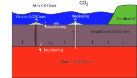
Figure 1.— Tidally-driven tectonism and pCO₂ long-term feedbacks. Continuous volcanism from a partially molten mantle degasses CO₂ in the ocean/atmosphere. The basaltic layer that forms from this volcanism can sequester C from the ocean/atmosphere reservoir via sea weathering. The basaltic crust grows at the top with resurfaced basalt, and founders at the bottom moving C into the mantle. There is no need for continents, and continental weathering, for this mechanism to enable the C-Si cycle on tidally heated planets.

Planets that are tidally heated can dissipate heat in their interior exhibiting partially molten mantles, that get rid of their heat by pushing melt through plumes to the surface. This melt continuously resurfaces in the form of basalt, and forms a layer that accumulates over time. This freshly advected rock can react with atmospheric or ocean CO₂ in a similar way to that on Earth and sequester C via a weathering reaction. With time, new basaltic crust gets deposited on top, so that the old basalt and carbonate rock get buried and move deeper within the planet. At some point, depending on the resurfacing rate, these rocks that were once at the surface will be buried and delaminated into the mantle, carrying down carbon with them and closing the cycle. Thus, recycling occurs in a vertical fashion instead of the horizontal character of plate tectonics on Earth.

We shall examine in more detail each of the components of this proposed system before presenting the climate model we built for these planets.

2.1.1 Tidal Heating

For a planet with a continuous and substantial source of tidal heating, the planet may have a partially molten interior . Just like the volcanism on Io, this melt may reach the surface through plumes advecting heat out to the surface. It is thus important to calculate the amount of heating a planet can experience. Based on the theory of tides (Murray & Dermott, 1999) the tidal heating available to a planet depends on the eccentricity of the system $e$, the semi-major axis $a$, the mass of the star $M_{\star}$, the mean motion $n$, the radius of the planet $R_{p}$, the specific dissipation parameter $Q$, the ratio of elastic to gravitational forces $\bar{\mu}$ $\left(\approx(10^{4}\mathrm{km}/R_{p})^{2}\right)$ and the gravitational constant $G$:

$$\frac{dE}{dt}=\frac{63}{4}\frac{e^{2}n}{\bar{\mu}Q}\left(\frac{R_{p}}{a}\right)^{5}\frac{GM_{\star}^{2}}{a}.$$ (1)

The least well constrained parameter is $Q$ although typical values of $\sim 100$ are commonly used for icy/rocky planets. In reality the dissipation parameter is a function of the planet’s structure and should vary radially instead of being a single value. However, as a first step, we use the same approach as in most studies and use a constant value. Equation 1 can also be written as

$$\frac{dE}{dt}\approx 10\times\left(\frac{e}{0.01}\right)^{2}\left(\frac{100}{Q}\right)$$ (2)

$$\left(\frac{R_{p}}{R_{E}}\right)^{7}\left(\frac{M_{\star}}{M_{\odot}}\right)^{5/2}\left(\frac{0.1\mathrm{AU}}{a}\right)^{15/2}[\mathrm{TW}].$$

Therefore, an Earth-sized planet orbiting a Sun-like star at $0.1$ AU and low eccentricity of $0.01$, would dissipate 10 TW or $\sim 0.02$ W/m², a tidal heatflux 100 times less than Io’s flux (Veeder et al., 1994; Spencer et al., 2000). For comparison, Earth’s flux is estimated at $0.09$ W/m² (Davies & Davies, 2010). To reproduce the measured heat flux for Io at its location with respect to Jupiter with Eq. 1, the dissipation factor would have to be chosen to be $Q_{\mathrm{Io}}=150.$

Given that we are interested in planets in the habitable zone that can experience tidal heating, we need to consider planets around M or even Brown Dwarfs. Planets around G type stars that are in the habitable zone, are too far away to experience any tidal heating from the star, whereas M stars have their habitable zone close enough that tidal dissipation can matter. In fact, tidal dissipation in planets around M dwarfs has been previously studied in the context of orbital and thermal evolution (Driscoll & Barnes, 2015). In fact, Barnes et al. (2009) claimed that there is a limit to how much tidal heating a habitable planet may experience based on the assumption that too much volcanism and high resurfacing rates would be inhospitable. In contrast, we propose that at these conditions, a new mechanism for climate regulation may kick-in rendering the planet habitable.

For a star with $M_{\star}=0.08\,M_{\oplus},$ like Trappist-1, an Earth-sized planet orbiting at $0.02$ AU and $0.01$ eccentricity would experience $3000$ TW or 6 W/m² of tidal energy. For an assumed eccentricity of 0.01 planets d and e would have a tidal flux of 0.96 and 0.30 W/m², respectively. These numbers quickly grow with eccentricity, so that planets around M stars can have large tidal heating fluxes. The important aspect for the model we propose is to determine if there is enough energy to yield a partially molten mantle. One could use Io for a simple comparison to infer whether or not planets like Trappist-1 $d,e$ and $f$ could have a partially molten mantle by comparing the amount of tidal energy available to the tidal energy carried to the surface.

Tidal production according to Eq. 1 increases as $R_{p}^{5}$, while the heat flow carried from the mantle to the atmosphere increases as $R_{p}^{2}$, so that at zero order larger planets should be more likely to have an interior melt region. Even at very low eccentricity values of $0.01$, Trappist 1d would experience similar tidal heat fluxes to that of Io. Thus, it is possible that the Trappist-1 planets in the habitable zone have persistent melt in their interior.

This melt would be advected in the form of volcanic conduits cooling at the surface, carrying with it volatiles and degassing them into the ocean/atmosphere (see Fig. 1). This continuous basalt extraction would form a layer of a certain thickness, limited by a partially molten mantle at the bottom. To estimate both the thickness of the basalt layer and the resurfacing velocity that are used in the climate model we use the model by O’Reilly & Davies (1981).

The resurfacing velocity, taken to be the same as the subsidence velocity, is

$$v=\frac{q_{t}}{\rho\left(L+C_{p}\Delta T\right)},$$ (3)

where $q_{t}$ is the tidal heat flux (tidal energy per unit surface area), $\rho$ is the density of the mantle, $L$ the latent heat, $C_{p}$ the heat capacity, and $\Delta T=T_{m}-T_{s}$ the difference between the melting and surface temperature. The thickness of the basalt layer is

$$d_{\mathrm{bas}}=\frac{\kappa}{v}\log\left(1+\frac{kv}{\kappa}\frac{\Delta T}{q_{t}\left(\frac{1}{a}-1\right)}\right),$$ (4)

where $\kappa$ is the thermal conductivity, $k$ is the thermal diffusivity, and $a$ is the ratio of tidal heat flux to total heat flux. While the resurfacing rate depends only on the tidal heat flux, the thickness of the basalt layer is also determined by the contribution of tidal energy flux to total flux, $a$, which is unknown. To illustrate this point, we have calculated the resurfacing velocity and basalt layer thickness for different values of $a$. Figure 2 shows what this thickness would be as a function of contribution of tidal heat to the total heat flux. As tidal heating becomes the dominant source (i.e. $a$ approaches $1$) the thickness becomes infinitely large (as shown by O’Reilly & Davies (1981)) We have also set a minimum contribution by considering steady state where the total heat flux is from tidal heating and radioactive decay. By setting a maximum to the radioactive decay of $2$ W/m² calculated from radioactive sources on Earth at 3.8 By ago, we obtain a minimum value of $a$. Trappist-1$d$, with a calculated tidal flux of $\sim 1$ W/m² according to this simple model, would have resurfacing velocities of 6 cm/y and a crustal layer of at least 2 km.

However, without a detailed calculation for the thermal history of these planets, which is beyond the scope of this paper, it is not possible to know how much of the total flux is coming from tidal heating, so as a simple first step we take $v$ and $d_{bas}$ to be set independent of each other.

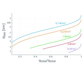
Figure 2.— Basaltic layer thickness as a function of ratio of tidal heat flux to total heat flux for different values of tidal heat flux. The corresponding resurfacing velocities are 0.6, 1.2, 6.0, 12, and 60 cm/y for tidal fluxes shown in figure from 0.1 to 10 W/m², respectively. The contribution of tidal heat flux to total heat flux $a$ depends on the thermal evolution of the planet.

Melt

Our model also requires melt to be continuously advected to the surface, which depends on how deep the melt is produced, and the chemistry of the melt. On Earth, due to plate tectonics, as upper mantle material adiabatically ascends into mid-ocean ridges, decompression melting takes place near the surface and melt gets carried out as volcanism. However, if melt is produced at depth, due to the crossover density of melt and solid at pressures of $\sim 13$ GPa or $\sim 350$ km on Earth, melt can stay within the mantle (Ohtani et al., 1995). In fact, Noack et al. (2017) has argued on the basis of this crossover density that stagnant-lid planets with large masses, or large core-mass fractions would not exhibit volcanism – owing to larger surface gravities, the pressure for the crossover density would be reached at shallower depths. This could pose a problem for our proposed mechanism if tidal dissipation creates melt deeper than the crossover density for the specific planet. The pressure for this crossover density depends on the composition of the solid (e.g. basalt versus peridotite, or iron content), and the water content of magma (Sakamaki et al., 2006). The higher the iron content of the solid or drier the magma, the shallower the crossover density. Sakamaki et al. (2006) shows that for Earth, hydrated magma occurring from melting mid-ocean ridge basalt rock has a crossover density near $410$ km ($\sim 24$ GPa ) if water is present at the 2% level, and deeper at the 8% level. By extrapolating their data and using the preliminary reference earth model (Dziewonski & Anderson, 1981), we obtain a crossover density depth for 8% water in magma of $1400$ km ($\sim 60$ GPa) for Earth. Given as well that tidal strain is largest near the surface, it is reasonable to think that tidal heating may produce melt near the surface, and thus our proposed mechanism may work for a subset of planets.

2.1.2 Sea Weathering

In broad strokes, the carbon-silicate cycle is the process by which CO₂ is drawn from the atmosphere by removing C when interacting with silicate rocks via water and carbonic acid that releases bicarbonate, Ca⁺⁺ (and Mg⁺⁺) ions either on the continents or interacting directly with basalt on the newly formed ocean crust. If on the continents, these ions eventually find their way to the ocean floor carried down by rivers and ground water. On the ocean floor they form carbonates that trap carbon (that was once in the atmosphere) into rocks, that eventually get subducted into the mantle at convergent margins. The net reaction is captured in the Urey reaction (Urey, 1952):

$$\mathrm{CO_{2}(g)+CaSiO_{2}(s)\Longleftrightarrow SiO_{2}(s)+CaCO_{3}(s)},$$ (5)

where the right arrow describes how carbonates are formed. Once at depth these carbonate rocks can react back via metamorphism, releasing carbon dioxide that eventually makes it back in to the atmosphere via volcanism (the reverse reaction, left arrow).

On Earth, this cycle is enabled by plate tectonics that continuously exposes fresh rock on the ocean floor, as well as on the continents driven by erosion via orogeny and topography build-up. Rock weathering has been well studied (Walker et al., 1981; Berner & Caldeira, 1997; Berner, 2004) while sea weathering has gained more traction in recent years (Coogan & Gillis, 2013; Coogan & Dosso, 2015). The carbonate reactions of sea weathering may be controlled in a different manner to continental weathering with secondary carbonates and alkalinity playing an important role (Coogan & Dosso, 2015). It is yet unknown the contribution of each weathering type to the total weathering process on Earth, or how it might have changed throughout Earth’s history (Mills et al., 2014). Although, recent estimates by Krissansen-Totton & Catling (2017) suggest that continental weathering has been dominant in the last 100 My.

For the planets proposed here, we envision that tidally-driven tectonism can continuously expose fresh rock under an ocean, but that any continental shelves, if present, may not exhibit rock weathering owing to a sustained lack of erosion. In this case, the only mechanism for drawing down CO₂ in these planets would be sea weathering.

While some authors have considered sea weathering as dependent on CO₂ concentrations alone (Sleep & Zahnle, 2001; Foley, 2015), laboratory experiments (Brady & Gíslason, 1997) and isotopic constraints from oceanic carbonates (Coogan & Dosso, 2015) suggest a temperature dependence in the form of an arrhenious law. This dependence on the deep ocean temperature, where Ca leaching, and carbonate production are taking place depends in turn, on the atmospheric temperature, and hence the atmospheric CO₂ concentrations, because atmospheric temperature determines how much cold surface water enters the thermohaline circulation system (Brady & Gíslason, 1997). This sea weathering dependence on atmospheric temperature and CO₂ is crucial in allowing for a climate stability feedback. We adopt the same equation as Mills et al. (2014) to describe sea weathering as a function of atmospheric CO₂ levels and atmospheric temperature $T$

$$W_{sea}=\omega W_{sea}^{E}\left(\frac{p\mathrm{CO_{2}}^{atm}}{p_{E}}\right)^{\alpha}\exp\left(\frac{E}{R}\left(\frac{1}{T_{E}}-\frac{1}{T}\right)\right),$$ (6)

where $R$ is the gas constant, $E$ is the activation energy, $W_{sea}^{E}$ is the sea weathering rate baseline estimate (in bar/My or mol/My) for a reference state that we set at first to be the equilibrium atmospheric partial pressure of carbon dioxide $p_{E}$, and atmospheric equilibrium temperature $T_{E}$, and $\omega$ is a function that lumps all other quantities that sea weathering might depend on. The feedback mechanism comes from the dependency on atmospheric temperature. Any deviations from the equilibrium temperature would drive much higher or lower levels of sea weathering depending on whether the planet is hot with high levels of atmospheric CO₂ or cold, respectively.

In addition, sea weathering may include a dependency (through $\omega$) on the velocity at which fresh rock is exposed, which in the case of the Earth is the ridge spreading velocity, which has has changed over time. For Earth this term is often written as $\omega=\left(\frac{v}{v_{\oplus}}\right)^{\beta}$, where $v_{\oplus}$ is the present day velocity. While many authors (Sleep & Zahnle, 2001; Mills et al., 2014; Foley, 2015) use $\beta=1$, Krissansen-Totton & Catling (2017) propose $\beta\sim 0.5$. In either case, this contribution is of order unity. Other factors may also be affecting weathering rate (e.g. alkalinity, grain size, etc), and thus for simplicity we take $\omega\sim 1$; or conversely our results for sea weathering can be taken as scaling with $\omega$.

Two terms in Eq. 6 are poorly known, the direct dependence on atmospheric carbon dioxide pressure $\alpha$ and the activation energy $E.$ Brady & Gíslason (1997) proposed $\alpha=0.23$ and $E=41$ kJ/mol, while Coogan & Dosso (2015) proposed $E=92$ kJ/mol, and Krissansen-Totton & Catling (2017) considered a range of $E=40-110$ kJ/mol. We vary both $\alpha$ and $E$, as well as perform a stability analysis to see the effect on the climate stabilizing feedback we propose here.

Alkalinity

Coogan & Dosso (2015) have argued that carbonate mineral precipitation is largely controlled by alkalinity, and the fact that rock dissolution involved in sea weathering increases alkalinity, the effect is to efficiently drive carbon sequestration. We note that Eq. 6 does not have an explicit dependence on alkalinity, but an implicit one, as it depends on global temperatures that influence deep water ocean temperature, which in turn controls the dissolution rates of mafic and ultramafic rocks (Krissansen-Totton & Catling, 2017).

2.2. Governing Equations

2.2.1 Carbon cycle

To build our carbon cycle model we divide our planet into distinct reservoirs: the mantle, basalt layer, and treat the ocean and atmosphere together (similar to (Sleep & Zahnle, 2001; Foley, 2015)). See Fig. 1 for a cartoon representation of the tectonic process we propose in this study.

Magmatic volcanism originates in the molten mantle layer and carries melt within pipes that outgas CO₂ into the ocean and atmosphere reservoirs at a rate proportional to the resurfacing rate $v$. The flux of CO₂ degassed into the atmosphere-ocean reservoir is

$$D=p\mathrm{CO_{2}}^{man}\left(\frac{fvA_{p}}{V_{man}}\right),$$ (7)

where $p\mathrm{CO_{2}}^{man}$ is the partial pressure of carbon dioxide in the mantle, $V_{man}$ is the volume of the mantle, $A_{p}$ is the area of the planet, and $f$ is the fraction of CO₂ within the melt that gets outgassed. On the other hand, the sink for the atmosphere-ocean reservoir is the flux of CO₂ that is weathered at the bottom of the ocean. Namely, the sea weathering rate described in Eq. 6. By drawing out CO₂ from the ocean, sea weathering effectively draws out CO₂ from the atmosphere given that the partitioning between the two reservoirs is set by how soluble CO₂ is. Following Foley et al 2015, we use Henry’s law for solubility to determine how much CO₂ is in the atmosphere ($p\mathrm{CO_{2}}^{atm}$) versus the ocean ($p\mathrm{CO_{2}}^{oc}$),

$$p\mathrm{CO_{2}}^{atm}= \,p\mathrm{CO_{2}}^{atm+oc}-p\mathrm{CO_{2}}^{oc}$$ (8)

$$= \,\frac{K_{H}}{\mu_{\mathrm{CO_{2}}}}\frac{p\mathrm{CO_{2}}^{oc}}{\left(\frac{p\mathrm{H_{2}O}}{\mu_{\mathrm{H_{2}O}}}+\frac{p\mathrm{CO_{2}}^{oc}}{\mu_{\mathrm{CO_{2}}}}\right)},$$

where $K_{H}$ is the solubility constant, $p\mathrm{H_{2}O}$ is the content of water in the ocean, and $\mu$ is the molar mass. The content of water in the ocean is calculated by assuming the mass of the Earth’s ocean $M_{oc}$.

While sea weathering is a sink for the atmosphere-ocean reservoir, it behaves like a source for the basaltic crust. Once C is sequestered into the basalt layer, it starts getting buried by subsequent melt deposited at the top. The C subsides until it reaches the bottom of the basalt layer, at which point it is delaminated into the molten mantle layer. To keep all the quantities in the same metrics, we use C and CO₂ interchangeably knowing that C resides in rocks, while CO₂ is gaseous form (degassing from mantle).

The rate at which CO₂ in the basalt is foundered or delaminated into the mantle is

$$F_{found}=p\mathrm{CO_{2}}^{bas}\frac{v}{d_{bas}}.$$ (9)

Therefore the carbon-dioxide source for the mantle is the carbon dioxide foundered from the basalt layer, and the sink is the flux being outgassed through volcanism. Thus, the equations describing this system are

$$\frac{d}{dt}p\mathrm{CO_{2}}^{atm+oc} =D\left(p\mathrm{CO_{2}}^{man}\right)-W_{sea}\left(p\mathrm{CO_{2}}^{atm},T\right)$$ (10)

$$\frac{d}{dt}p\mathrm{CO_{2}}^{man} =F_{found}\left(p\mathrm{CO_{2}}^{bas}\right)-D\left(p\mathrm{CO_{2}}^{man}\right)$$

$$\frac{d}{dt}p\mathrm{CO_{2}}^{bas} =W_{sea}\left(p\mathrm{CO_{2}}^{atm},T\right)-F_{found}\left(p\mathrm{CO_{2}}^{bas}\right)$$

.

Given that the total content of CO₂ for the planet is fixed $p\mathrm{CO_{2}}^{atm+oc}+p\mathrm{CO_{2}}^{man}+p\mathrm{CO_{2}}^{bas}=p\mathrm{CO_{2}}^{tot}$, one of the three equations is redundant.

The equilibrium carbon dioxide values for the mantle, atmosphere and ocean are

$$p_{E}^{man}=W_{sea}^{E}\frac{V_{man}}{fvA_{p}}$$ (11)

$$p_{E}^{ao}=p\mathrm{CO_{2}}^{tot}-W_{sea}^{E}\left(\frac{d_{bas}}{v}+\frac{V_{man}}{fvA_{p}}\right)$$ (12)

and $p_{E}^{oc}=p_{E}^{ao}-p_{E}$ in dimensional form.

For typical values refer to Table 1. To be able to solve the system of equations 10 or A9, we need to specify the equilibrium conditions for the atmosphere, namely the equilibrium partial pressure of CO₂, $p_{E}$, that sets the equilibrium atmospheric temperature. While Menou (2015) took $p_{E}=330$ $\mu$bar , the pre-industrialization carbon dioxide partial pressure as the equilibrium value for the Earth, Haqq-Misra et al. (2016) argued that a more appropriate value for an abiotic Earth would be $p_{E}=0.01$ bars, by including all the carbon dioxide presently stored in the soil. We also take the equilibrium partial pressure to be $p_{E}=0.01$ bars.

This value for the atmosphere, the solubility constant for the ocean, and the amount of water in an Earth’s ocean, set the equilibrium CO₂ value for the atmosphere-ocean system via Eq. 8 to be $p_{E}^{ao}=0.038$ bars.

We also note that in line with astrophysical studies we use the units of bars instead of moles, and the conversion factor we use is

$$p\mathrm{CO_{2}}[\mathrm{bars}]=1.019710^{5}\times\mu_{\mathrm{CO_{2}}}\frac{g}{4\pi R_{p}^{2}}\times\mathrm{C}\quad[\mathrm{moles}],$$ (14)

where $g$ is the planet’s gravity and $R_{p}$ is the planet’s radius.

2.2.2 Climate Model

To obtain the atmospheric temperature of a planet provided the carbon dioxide partial pressure, we use the energy balance model (EBM) by Haqq-Misra et al. (2016). They provide a fit to the outgoing longwave radiation ($OLR$), and top of the atmosphere Bond albedo for four different type of stars including G and M stars. These quantities depend on the atmospheric carbon dioxide partial pressure, temperature, and zenith angle $\mu$. We simplify the model to capture global parameters by fixing the zenith angle to a value $\mu=0.232$ that would provide a global surface equilibrium temperature of $T_{E}=288$ K for $p_{E}=0.01$ bars for an Earth-like scenario. The zeroth-order energy balance model we use equates the planet’s thermal radiation to the net insolation

$$OLR(p\mathrm{CO_{2}}^{atm},T)=\frac{S_{\star}}{4}\left(1-A\left(p\mathrm{CO_{2}}^{atm},T\right)\right),$$ (15)

where $S_{\star}$ is the solar constant at the planet’s location, and $A$ is the top of the atmosphere albedo. This quantity also depends on the ground albedo which we take from Williams & Kasting (1997) and modify it for M stars. For the Earth, the ground albedo is taken to be a discontinuous function of $T$, where for temperatures less than $273$ K, the ground is considered to be frozen and exhibit a high albedo. At temperatures below $263$ K the water in the atmosphere is assumed to condense out entirely owing to the abrupt transition of the Earth entering a snowball state. However, a recent study by Checlair et al. (2017) on planets around M stars suggests that unlike on Earth, ice coverage would proceed gradually, avoiding sudden snowball transitions, owing to the special spatial insolation pattern they receive. In our model, we use both the same albedo function for Earth as well as a modified version that precludes the snowball state following Checlair et al. (2017). To achieve this, we allowed for a gradual ice coverage as temperatures decrease below 273, retaining 30% of the land exposure at 150 K, and allowed for cloud albedo at all temperatures.

The timescale governing Eq. 15 is much faster than the long geophysical timescale involved in the carbon-silicate cycle of Eqs. 10 (Menou, 2015). This means that in our model, surface temperature is calculated instantaneously from the amount of $p\mathrm{CO_{2}}^{atm}$ at each timestep in the integration of Eqs. 10.

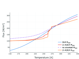
Figure 3.— Energy Balance Model. Insolation at the location of the habitable zone (orange) for G stars, (red) M stars and (purple) M star without snowball states is balanced by the outgoing long-wave radiation OLR (blue) setting the temperature at the surface for $p\mathrm{CO_{2}}=0.01$ bars.

Figure 3 shows the results from the EBM model for the equilibrium case $p\mathrm{CO_{2}}^{atm}=0.01$ bars. We show the case of the Earth (orange line) for comparison purposes. Earth’s climate exhibits two stable points, one near 225K where the planet would be in a snowball state, and the temperate 288K, as well as one unstable point, near 273K. Furthermore, the snowball state at 225K is thought to be transient, given that rock weathering is considered to be suppressed at these temperatures so that outgassing from volcanoes eventually deglaciates the planet. It is worth mentioning that if sea weathering can operate at these cold temperatures in a large enough way as to balance volcanism, this snowball state could be stable on long term timescales. Sea weathering would have to happen on the ocean floor below a thick crust of ice, that still allows for carbon dioxide to diffuse from the atmosphere to the ocean, and volcanism would most likely have to be sluggish.

Considering planets around M dwarfs we also modified the EBM to restrict snowball states. This results in allowing for only one stable temperature state (purple line).

2.2.3 Stellar Evolution

We investigate whether an adequate surface temperature can be kept during the evolution of an M star for billions of years after the first 1 active billion. Compared to G type stars like our Sun that brighten over time after hydrogen ignition takes place, M stars get dimmer. This means that the habitable zone moves in with time, and hence, planets that are found in the habitable zone where once too hot. This raises issues as to the likelihood of these planets to be desiccated or wet after the intense EUV/XUV star fluxes. While earlier studies (Barnes et al., 2013) estimated planets around M dwarves to be completely dry, recent works (Bolmont et al., 2017; Schaefer et al., 2016) that use a better prescription for the atmospheric loss (Tian, 2015), suggest that some water is retained, making them prospective planets for habitability.

For the evolution of an M dwarf, we use a spline fit to the model by Baraffe et al. (2015) for a star of mass $M_{star}=0.08\,M_{Sun}$ like Trappist-1. Figure 4 shows the evolution of Trappist-1 compared to that of our Sun.

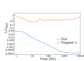
Figure 4.— Stellar evolution tracks used. The brightness of the M dwarf (blue) decreases over time, while the Sun (orange) has been brightening since it reached the main sequence.

3. Results

3.1. Sea Weathering

We look first at how an equilibrium may be established and the timescale associated with it. All the values for the parameters used in the model are shown in Table 1.

To integrate Eqs. 10 we can proceed in either of two following ways: 1) determine the sea weathering rate needed to ensure the equilibrium of the system is at $p_{E}=0.01$ bars and $T_{E}=288$ for the carbon content of the planet , and compare this weathering rate to values obtained for Earth, or 2) use Earth’s estimated weathering rate at present day conditions of pCO${}_{2}^{atm}=0.01$ and $T=288$ K to be the reference state in Eq. 6, include the term for velocity, for other planets, derive the corresponding equilibrium states, and then ask if they are suitable for surface liquid water.

In either case, the functional form of the governing equations remains the same, and from stability analysis (see Appendix) we conclude that the equilibrium state is in fact stable.

We use both approaches but favour the first one to solve for the equations for two reasons. We use a simple functional form for sea weathering that could be made more realistic with more understanding (e.g. alkalinity dependence, etc), and there is considerable uncertainty behind calculating present day sea weathering rates. Values used previously range by more than one order of magnitude from 0.225-0.675 Tmol C/year (Krissansen-Totton & Catling, 2017), 1.75 Tmol C/year (Mills et al., 2014) and 3.4 Tmol C/year (Alt & Teagle, 1999; Sleep & Zahnle, 2001). Thus, we are not confident enough in our understanding of sea weathering rates on Earth to use it at face value for other planets.

To ensure the equilibrium conditions of $p_{E}=0.01$ bars and $T_{E}=288$ are at met, the sea weathering at equilibrium must adjust itself to account for the planetary tectonic conditions and the total carbon dioxide content in the following way

$$W_{sea}^{E}=\left(p\mathrm{CO_{2}}^{tot}-p_{E}^{ao}\right)\frac{fvA_{p}}{\left(V_{man}+fA_{p}d_{bas}\right)}.$$ (16)

If this sea weathering rate can be achieved, and there are no limiting processes hindering sequestration (i.e. reaction kinetics), then equilibrium conditions suitable for water on the planet’s surface are possible. Figure 5 shows how the sea weathering at equilibrium varies as a function of total carbon dioxide content for different resurfacing velocities and basaltic crust thicknesses.

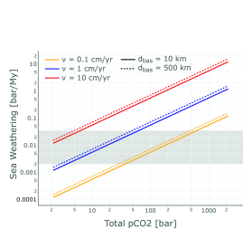
Figure 5.— Equilibrium Sea Weathering. The rate of uptake of CO₂ in the ocean crust needs to adjust to values that depend on the thickness of the basaltic layer (dash for 10 km and dotted for 500 km) and the resurfacing velocity (yellow: 0.1 cm/yr, blue: 1 cm/yr, red:10 cm/yr) for a given total carbon content. The shaded region shows an estimate on the range of today’s present day values according to (Krissansen-Totton & Catling, 2017; Mills et al., 2014; Alt & Teagle, 1999; Sleep & Zahnle, 2001).

We consider the total planetary carbon content to be the same as for Earth estimated at $2.5\times 10^{22}$ moles C/yr(Sleep & Zahnle, 2001) or $215.51$ bars. Io’s estimated resurfacing rate is 0.55-1.06 cm/yr (McEwen et al., 2004a) to a few cm/yr (Phillips et al., 2000) and crustal thickness is $14$ km$-30$ km at a minimum (Jaeger et al., 2003; Carr et al., 1998). We take as our fiducial case a resurfacing velocity of $v=1$ cm/yr and basaltic crust layer thickness $d_{bas}=10$ km, in alignment with Io, which yield an equilibrium sea weathering rate of $120$ bars/Gy. This is above the range estimated for present day Earth ($1.9-29$ bar/Gyr). For comparison, a less active planet, with a resurfacing rate of $v=0.1$ cm/y, would require equilibrium sea weathering rates of $12$ bar/Gy, well within present day Earth’s estimates.

It is clear that the most important factor is the carbon content of the planet and the resurfacing velocity. The shaded region shows present day estimates for sea weathering rate on Earth.

If there is a limit to how much sea weathering can take place, for a given total carbon content then lower resurfacing velocities are needed in order to have an equilibrium state, while the thickness of the basaltic layer is less important (see Fig. 5). In turn, resurfacing velocities depend on the tidal heat flux, or tidal forcing. Thus, if there is a limit to sea weathering, there will be a limit to tidal heating above which the planet will not exhibit an equilibrium atmospheric state over long timescales that favours liquid water. It is beyond the scope of this paper to calculate the exact limits, as this would require building a thermal evolution model for the planet.

Likewise, for a given resurfacing rate set by tidal heating, planets with less amount of C are favoured in maintaining surface habitable conditions via tidally-induced tectonism.

If instead, we take Earth sea weathering value $W_{sea}^{\oplus}$ at face value and valid only in the reference state, we can calculate the equilibrium conditions for atmospheric temperature and CO₂ pressure for other planets. For this case we make explicit the dependence on the velocity by setting $\omega=\frac{v}{v_{\oplus}}$ and take $v_{\oplus}=3$ cm/y. We obtain the equilibrium conditions for a given set of resurfacing velocities, basaltic layer thicknesses and total carbon content by solving for the value of $p_{E}$ that satisfies the equation

$$p_{\mathrm{CO_{2}}}^{tot}=p_{man}^{E}\left(1+\frac{fd_{bas}A_{p}}{V_{man}}\right)+p_{E}+p_{\mathrm{CO_{2}}}^{oc}(p_{E})$$ (17)

given that,

$$p_{man}^{E}=\frac{V_{man}}{fvA_{p}}W_{sea}^{\oplus}\frac{v}{v_{\oplus}}\left(p_{E}/p_{\oplus}\right)^{\alpha}\exp\left(\frac{E}{R}\left(\frac{1}{T_{\oplus}}-\frac{1}{T_{E}}\right)\right)$$ (18)

Figure 6 shows the range of equilibrium temperature values as a function of different planetary carbon contents, for an Earth’s average spreading rate of $v_{\oplus}=3$ cm/y and three different estimates of Earth’s sea weathering rate: $W_{sea}^{\oplus}=0.55$ Tmol/y = 1.9 bar/Gy (Krissansen-Totton & Catling, 2017) , $W_{sea}^{\oplus}=1.75$ Tmol/y = 15 bar/Gy (Mills et al., 2014) , and $W_{sea}^{\oplus}=3.4$ Tmol/y = 29 bar/Gy (Sleep & Zahnle, 2001). It can be seen that planets with modest amounts of total carbon can achieve habitable conditions easier than those that have more carbon content. For example, planets with carbon contents a few times that of the Earth can have liquid water (shaded region) when assuming a 1 bar atmosphere, albeit at hotter conditions.

Either way of calculating sea weathering, it is clear that planets with low carbon contents, and/or sluggish resurfacing velocities are favoured for exhibiting a carbon-silicate cycle that keeps the atmospheric temperature at habitable conditions.

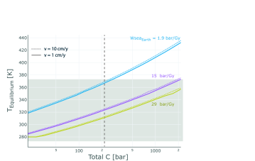
Figure 6.— Equilibrium surface temperature for planets with different C contents provided three sea weathering rates estimates for the Earth, blue: 1.9 (Krissansen-Totton & Catling, 2017) , purple: 15 (Mills et al., 2014), and green: 29 bar/Gy (Sleep & Zahnle, 2001), and spreading rate of $v_{\oplus}=3$ cm/y. Dashed line corresponds to the estimated C content for the Earth according to Sleep & Zahnle (2001). The shaded region shows conditions for liquid water provided a 1 bar atmosphere.

3.2. Equilibrium Timescale

Having established the equilibrium conditions, we proceed to solving the governing equations. Our approach is to set the sea weathering rate to a value that allows for an equilibrium similar to the Earth with $p_{E}=0.01$ bar and $T_{E}=288$K. However, the behaviour is expected to be qualitatively similar had we used fixed the sea weathering rate to the Earth’s value given the same functional form of the Equations.

We first start with a fixed present day Sun to find out how long it takes to reach the equilibrium state and how it changes with different parameters. As initial conditions we tested different ones (similar to those used by Foley (2015)) and show only the most extreme case of disequilibrium where there is no carbon in the mantle to begin with. While this case is not really realistic it stand to show that the system can recover equilibrium even for these extreme beginnings. We consider the cases where a) these planets reach snowball states and b) where they do not. We vary the initial atmospheric CO₂ values to allow for cold or hot beginnings.

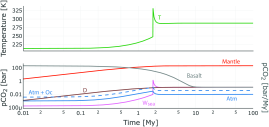
Figure 7.— CO₂ evolution towards equilibrium for tidally heated planets in the habitable zone. Temperature (top, green) changes as the partial pressure of atmospheric CO₂ (blue) evolves. The CO₂ content of the atmosphere+ocean reservoir (dashed blue) evolves commensurate with the atmospheric CO₂ partial pressure given an assumed solubility independent of temperature. The C content in the basalt (grey) and mantle (red) reach the equilibrium state at a few tens of My once the sea weathering rate (pink, in bar/My) and volcanic degassing (brown, in bar/My) reach parity.

Figure 7 shows how the system reaches equilibrium starting from a cold state. With no C in the mantle, the system initially starts with no outgassing into the atmosphere. With cold temperatures ($T=215.5$ K for $p_{0}^{atm}=0.001$), the weathering rate is very small and draws down little amount of CO₂ from atmosphere (and ocean) into the basaltic layer that starts as a rich C reservoir. Foundering from this basaltic crust slowly starts building the mantle’s C reservoir, as outgassing is outpaced. This little outgassing slowly builds up more CO₂ in the atmosphere, so that it heats up and starts melting the ice on the surface. At some point there is enough CO₂ in the atmosphere that the planet deglaciates completely, this changes the albedo suddenly to much lower values and the planet transitions into a hot state (the only permanent stable point in the EBM plus evolution equations is at high temperatures). The system overshoots from the equilibrium point because too much CO₂ had built in the deglaciation phase. This overshoot is controlled by the rate of outgassing and the time it has taken the planet to deglaciate. At this very hot state, the sea weathering rate increases by an order of magnitude and quickly draws back down the excess CO₂ in the atmosphere, all the while decreasing C in the basaltic crust and increasing it in the mantle, relaxing into the equilibrium state. Analogous behaviour has been discussed in the context of Earth and deglaciating from previous snowball states (Hoffman & Schrag, 2002).

If we restrict the ice coverage of the planet to eliminate snowball transitions, following Checlair et al. (2017), then the inital state is less cold ($T=243$ K) and no overshooting happens. See Fig. 8 top panel. The planet just heats up until it reaches the equilibrium state. Discontinuities in the temperature come from discontinuities in the ground albedo as a function of surface temperature via the amount of land, snow and ice coverage that have been modelled in a simple fashion.

The last case we considered was a hot beginning with $p_{0}^{atm}=0.05$ bars (the hottest point allowed in the EBM model for M stars). The evolution from a snowball or no-snowball planet is the same. For this hot beginning, sea weathering starts at a high rate, drawing down CO₂ from the atmosphere, bringing down the surface temperature. In the meantime, the basaltic layer is foundering more C to the mantle than the mantle degasses, so that the mantle’s reservoir builds up. The system also slightly overshoots, but not to a point of glaciation, and then relaxes into the equilibrium state.

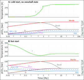
Figure 8.— CO₂ evolution towards equilibrium for tidally heated planets in the habitable zone. Top) Cold initial state for planets without snowball states. Bottom) Hot initial state.

We find that the timescale to reach equilibrium is about 10 -100 My and is independent of total CO₂ content, activation energy $E_{sea}$ values, or dependency of the sea weathering rate on the amount of atmospheric CO₂, $\alpha$. The factors that change this timescale are the crustal thickness $d_{bas}$, resurfacing velocity $v$, and outgassing rate. An order of magnitude increase in crustal thickness from 10 to 100 km increases the timescale by about one order of magnitude from $\sim 10$ to $\sim 100$ My. An increase in resurfacing velocity from 1 to 10 cm/yr decreases the timescale by about one order of magnitude. A decrease in outgassing fraction by one order of magnitude from $f=0.1$ to $0.01$, increases the timescale by a factor of a few.

While these relationships were obtained through parameter exploration, we also obtained an expression for the equilibrium timescale by non-dimensionalizing 10 (see Appendix). The expression is

$$\tau\simeq\frac{d_{bas}}{v\sqrt{f}}$$ (19)

On the other hand, larger values of total carbon inventories while not changing the timescale to reach equilibrium, may affect the timing of complete deglaciation (by a few My) while preserving the amount of overshoot in atmospheric CO₂ , and thus the atmospheric temperature (to about $330$ K). Different values of $v$ have the same effect on changing the timing of the overshoot, but not the peaks and troughs in temperature. Thus, for reasonable values for the parameters in the model, the timescale to reach equilibrium is 10-100 My. Therefore, shorter or longer time scale processes are not expected to affect the planet’s ability to sustaining equilibrium.

3.3. Long-Term Evolution

For completeness, along the same lines, we also looked at how a tidally-heated planet may evolve as the M star dims over time. Because the evolution of stars changes in a billion year timescale, we find the planets reaching equilibrium at 10-100 My, as expected. Thus, we only show the evolution case of a hot start as it is likely that planets that end up in the habitable zone around a M stars, started hot (unless there is some mechanism for migration that might have brought them from further out, a la Hansen & Murray (2012) ). To stay within the bounds of the EBM model by Haqq-Misra et al. (2016) our initial start is at $p_{0}^{atm}=0.033$ bars. After 10-100 My the CO₂ contents of the reservoirs reach the equilibrium state for the solar luminosity at the time. Given that the star is brighter in the past, the CO₂ content is lower ($p^{atm}=0.007$ at 2.9 By ago), while the atmospheric temperature ($T=289$ K) is slightly larger than present day. Our choice for starting the evolution 3 By ago is tied to the range in which the EBM model is valid. However, there is no reason to believe that this mechanism would not operate further into the past at larger insolation values. The limit would be set by reaching the runaway greenhouse. In other words, planets in the habitable zone of M dwarfs may start hot, with a steam atmosphere, that partially evaporates, while the star is active. As luminosity decreases, the remaining water in the atmosphere will condense out (Bolmont et al., 2017; Schaefer et al., 2016), or perhaps any water stored in the mantle can outgas to the surface. For planets located in near-resonant chains, which can keep eccentricities from decaying to zero, tidally driven tectonics may start taking place.

Our simple model shows that tidally-locked planets may have a built-in mechanism to regulate the amount of CO₂ in the atmosphere to allow for long term stability of surface liquid water, similar to Earth. However, unlike Earth’s carbon-silicate cycle that relies on plate tectonics, these tidally heated planets recycle material vertically via continuous volcanism and foundering.

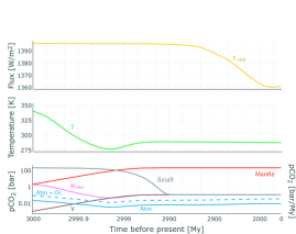
Figure 9.— CO₂ long-term evolution as the host M star evolves form an initial hot state

3.4. Sub-Earths and Super-Earths

A simple extension of this work is to consider planets that are less or more massive than Earth, while still being rocky. Low-mass exoplanets, including super-Earths are now known to be common in our galaxy (Howard et al., 2010). We consider planets that have the same major element composition as Earth, including the same core mass fraction and assume that these planets experience constant volcanism. We use parameters for planetary radius, gravity and core radius to account for the different mass according to the internal structure model by Valencia et al. (2006)

In terms of the planetary carbon inventory we consider two scenarios: 1) planets with same total C content as Earth , and 2) planets with the same C content per unit mass. In reality, due to the volatile character of carbon, we do not fully understand how Earth acquired the amount it has, and how to extrapolate this accurately to other terrestrial planets. Thus our two scenarios may be thought of as possibilities, from which we can draw a few conclusions.

We use the same resurfacing velocity and crustal thickness for all planets, independent of their mass as a first order approach. The timescale to reach equilibrium remains unchanged, although in the case of cold initial states with snowball transitions, the overshoot is delayed for larger planets. Thus, when considering only the effects of geometry and gravity, our proposed mechanism is robust.

Not surprisingly, when we allow planets’ carbon inventory to scale with mass, it affects the system’s requirements. If we require an equilibrium around T=288K, planets with lower carbon contents require more reasonable sea weathering rates (Fig. 10 top). If instead, we take Earth’s sea weathering at face value, smaller planets with lower carbon contents experience equilibrium temperatures that are temperate whereas large planets would be too hot (Fig. 10 top).

In general, in terms of a negative feedback mechanism that regulates surface temperature via CO₂ sequestration, there needs to be a balance between outgassing that depends on planetary carbon content and weathering. Thus, lower planetary carbon contents are favoured.

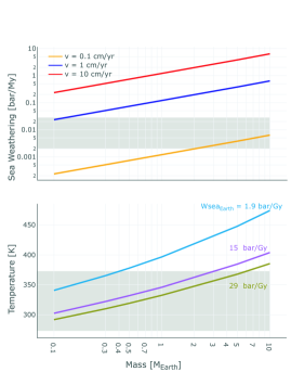
Figure 10.— Tidally driven tectonics in sub and super-Earths with scaled carbon content. Top: Sea weathering rates needed to ensure equilibrium of $T=288$K and pCO${}_{2}=0.01$ bars for planets of different masses and corresponding carbon contents. Bottom: Equilibrium surface temperatures if sea weathering rates are the same as the Earth given three different estimates ( same as in Fig 6)

Another aspect of planetary mass is how it affects the ability of the planet to advect melt to the surface given the fact that there is a crossover density at some pressure below which any melt produced is negatively buoyant and stays within the mantle (Ohtani et al., 1995). The depth at which this occurs depends on the gravity, and thus on planet mass. A simple gravity scaling based on Valencia et al. (2006), yields $g\simeq g_{E}\left(M/M_{E}\right)^{1/2}$, which translates to a depth scaling of $h\simeq h_{E}\left(M/M_{E}\right)^{-1/2}$. Thus, smaller planets are more likely to produce melt above the depth at which the crossover density happens. Following Sakamaki et al. (2006) and this simple scaling (which ignores compression effects) we obtain for a $10\,M_{E}$ planet (with the same core-mass fraction as Earth) depths for the crossover density of 110 km, 130 km, and 450 km for anhydrous magmas, hydrated magmas at the 2% and 8% level, respectively. For a $0.1\,M_{E}$ planet the corresponding depths are 1100 km, 1300 km, and beyond the core-mantle boundary of the planet. Thus, details about the composition of the mantle and melt as well as where tidal dissipation takes place are needed to establish exactly which planets will produce melt that can be advected to the surface, and sustain the mechanism we propose. These effects are beyond the scope of this paper, and left for future work. However, qualitatively, melt is more easily advected in smaller planets, with hydrated magmas, and thus making small wet planets more suitable to exhibit habitability from tidally heated tectonism.

Table 1Model Parameters

Parameter	symbol	value	Reference
Sea weathering dependence on CO2	$\alpha$	$0.23$	(1)
Sea weathering at equilibrium	$W_{sea}^{E}$	$0.12$ bar/My	calculated
Equilibrium atmospheric temperature	$T_{E}$	$288$ K	assumed
Equilibrium atmospheric CO2 partial pressure	$p_{E}$	0.01 bars	(2)
Activation Energy	$E_{sea}$	41 kJ	nominal value, (1)
Outgassing CO2 fraction	$f$	0.01	nominal value, assumed
CO2 molecular weight	$\mu_{\mathrm{CO}_{2}}$	$44.1$ mol/g	calculated
H2O molecular weight	$\mu_{\mathrm{H_{2}O}}$	$18.015$ mol/g	calculated
Mass Ocean	$M_{oc}$	$1.4\times 10^{24}$ kg
Solubility constant	$K_{h}$	$235.48$ bar	calculated
Planet Radius	$R_{p}$	$6371$ km	3
Core’s Radius	$R_{c}$	$3400$ km	3
Planet Mass	$M_{p}$	$5.972\times 10^{24}$ kg	3
Zenith angle	$\mu$	0.232	calculated
Sun’s luminosity today		1361 W/m2
Basalt crust thickness	$d_{bas}$	$10$ km	nominal value, assumed
Resurfacing velocity	$v$	$1$ cm/y	nominal value, assumed
Total carbon content	$p\mathrm{CO_{2}}^{tot}$	$215.51$ bars	4
Characteristic timescale	$\tau$	$3$ My	calculated

Refs: (1) Brady & Gíslason (1997), (2) Haqq-Misra et al. (2016), (3) Stacey & Davis (2008), (4) Sleep & Zahnle (2001)

4. Discussion

The simple model we propose has three elements at its core that make for the built-in thermostat: 1) the sea weathering rate depends sensitively on the atmospheric temperature (via controlling the temperature of the deep ocean), 2) the atmospheric CO₂ can be drawn out and sequestered into a reservoir when needed, and 3) this reservoir is connected back into releasing CO₂ into the atmosphere via outgassing, which in our proposed model happens via foundering of the basaltic layer into the mantle that, in turn, continuously outgases into the atmosphere by advecting melt onto the surface.

This model does not consider possible limits to the weathering rate. By construction we have invoked a mechanism that continuously exposes fresh basaltic crust available for weathering, in analogy to Earth. However, if volcanism is too infrequent on timescales that are longer than $\sim$10-100 My, it could be a problem for the system to maintain equilibrium. Brady & Gíslason (1997) noted that seafloor weathering on Earth seems to occur mostly within the first 3 My and stops after 10 My after crust production. Thus, for continuous sea floor weathering, enough volcanism should happen at most every $\sim$million year.

Also, incipient volcanism may limit the amount of weatherable material in a similar way to the transport-limited scenario explored by West et al. (2005); West (2012) for Earth. In the transport-limited regime, the replenishment of fresh Ca and Mg ions is the bottle neck to weathering. In the case of the Earth it can be due to low erosion rates (West et al., 2005; West, 2012). In rocky exoplanets it can be due to limited land exposures Foley (2015). In our case it can be due to limited volcanism. Including a transport-limited sea weathering rate, would impose a limit to the amount of total planetary carbon, and/or a resurfacing rates (which are dependent on tidal heating values) below which the planet has the ability to sequester C at a high enough rate to keep CO₂ atmospheric values below a greenhouse atmosphere. Thus, understanding better what parameters control sea weathering would help us determine how ubiquitous this kind of C-Si cycle can be in exo-Earths.

In addition, we treated seafloor weathering in the simplest way possible. For example, our equation for seafloor weathering lumps alkalinity into the surface temperature dependence, and thus we omit a treatment for ocean chemistry (Krissansen-Totton & Catling, 2017). These improvements are left for future work to bring focus to the main ingredients laid out in this study.

Our proposed scenario excluded the existence of rock weathering on continents. However, it may be that orogeny can happen as a secondary process to tidally induced volcanism as suggested on Io (McEwen et al. (2004b) and references therein). If so, weathering may proceed in both the continents and on the seafloor.

We note that in our modelling we have taken the parameters for the thickness of the basaltic layer and the resurfacing velocity as independent quantities, while in reality they are connected via the contribution of tidal heating to the total heat flux of the planet (factor $a$ in Eq. 4 ). We have taken this route because to properly assess this contribution one would have to model the thermal history of the planet including an accurate description of the tidal dissipation parameter $Q$, and the effect of melt on it, which is beyond the scope of this study.

Another refinement to our simple model may be to include the effects of phase transitions happening within the basaltic layer. On Earth, the basalt to eclogite transition may cause delamination within a thick crust and cool the surrounding mantle faster than otherwise, and limit the size of the basaltic crust. Including this effect on our model would require adding another layer between the basaltic crust and the mantle from which outgassing proceeds. Because of mass balance, adding another layer would not change the character of the equations, and thus the results presented.

Future work may be extended to include thermal history calculations, sweeping of parameter space for planets at different orbital configurations, different carbon contents, and include the effects of transport-limited sea weathering via limited volcanism.

If our proposed mechanism to regulate atmospheric CO2 takes place in planets like Trappist-1$d$ the CO₂ content in the atmosphere would be around values that would yield liquid water on its surface, namely $\sim 0.5$ bars, assuming the planet is abiotic. Indeed, if there is a negative feedback mechanism that enables a thermostat taking place in other planets, enabled by either the mechanism proposed here or by plate tectonics , or even perhaps in stagnant lid (Foley & Smye, 2017) the CO₂ content of the atmosphere has to be commensurate with insolation values, something we can test for with enough atmospheric data. However, because planets that are substantially tidally heated most likely are getting rid of heat via heat piping, we can be guided by estimates of the tidal dissipation from orbital dynamics to pinpoint whether or not we expect heat piping to occur instead of plate tectonics or stagnant lid.

5. Summary

In summary, we propose a new mechanism for rocky planets around M dwarfs to have a climate-controlling feedback mechanism that can keep liquid water stable for billions of years. An analogous carbon-silicate cycle can operate on planets by recycling carbon between the atmosphere, a basaltic crust and the mantle via tidally-induced volcanism, basaltic formation and sea weathering, plus foundering. In contrast to plate tectonics that enables the carbon-silicate cycle on Earth, these planets would achieve the same principle by recycling material vertically.

Continuous exposure of basaltic crust through volcanism can be weathered to sequester C from the ocean and atmosphere, to draw down CO₂ atmospheric levels when values are too high, or outgases CO₂ from the mantle to replenish atmospheric values when they are too low, as long as sea weathering depends on atmospheric temperature.

Therefore, the tidal properties of planets around M dwarfs, in the absence of plate tectonics, may enable stable climates suitable for habitability, making the search for these planets more attractive than it already is.

The equilibrium timescale of $\sim$ 10-100 Myr underlying this mechanism ($\tau\simeq d_{bas}/v\sqrt{f}$) is very different from the timescales for stellar brightness evolution or flares, thus remaining impervious to these changes.

This mechanism may be tested by retrieving atmospheric CO₂ values from nonzero eccentric planets in the habitable zone that are dissipating to much heat via pipe heating to exhibit plate tectonics. If this type of tectonism is happening and controlling climate, the values for CO₂ should be consistent with insolation values. Trappist-1 planets in the habitable zone may be an example.

Appendix A Linear Stability and Equilibrium Timescale

This system of ordinary differential equations that govern this system (Eq. 10) can be non-dimensionalized to yield

$$\frac{d}{dt^{{}^{\prime}}}p\mathrm{CO_{2}^{{}^{\prime}}}^{atm+oc} =\frac{W_{sea}}{p_{E}^{ao}}\tau\left(p\mathrm{CO_{2}^{{}^{\prime}}}^{man}-\left(p\mathrm{CO_{2}^{{}^{\prime}}}^{atm}\right)^{\alpha}\exp\left(\frac{E}{R}\left(\frac{1}{T_{E}}-\frac{1}{T}\right)\right)\right)$$ (A1)

$$\frac{d}{dt^{{}^{\prime}}}p\mathrm{CO_{2}}^{man} =\tau\frac{fA_{p}v^{2}}{V_{man}d_{bas}}\left(\frac{p_{E}^{ao}}{W_{sea}^{E}}\right)\left(1-p\mathrm{CO_{2}^{{}^{\prime}}}^{atm+oc}\right)+\tau\left(\frac{fvA_{p}}{V_{man}}+\frac{v}{d_{bas}}\right)\left(1-p\mathrm{CO_{2}^{{}^{\prime}}}^{man}\right)$$

with nondimensional variables

$$p\mathrm{CO_{2}^{{}^{\prime}}}^{atm+oc}=p\mathrm{CO_{2}}^{atm+oc}/p_{E}^{ao}$$ (A2)

$$p\mathrm{CO_{2}^{{}^{\prime}}}^{atm}=p\mathrm{CO_{2}}^{atm}/p_{E}$$ (A3)

$$p\mathrm{CO_{2}^{{}^{\prime}}}^{man}=p\mathrm{CO_{2}}^{man}/p_{E}^{man}$$ (A4)

$$p\mathrm{CO_{2}^{{}^{\prime}}}^{oc}=p\mathrm{CO_{2}}^{oc}/p_{E}^{ao}$$ (A5)

$$t^{{}^{\prime}}=t/\tau$$ (A6)

After inspection of the numerical results solving the dimensional equations, as well as combining both equations in LABEL:eq:nondim1 into a second order differential equation for $p\mathrm{CO_{2}^{{}^{\prime}}}^{man}$ and retaining the non derivative terms, we conclude that the most appropriate timescale is

$$\tau=\frac{1}{v}\sqrt{\frac{d_{bas}V_{man}}{fA_{p}}},$$ (A7)

which in the limit of a thin basaltic crust layer $d_{bas}/R_{p}\ll 1$ becomes

$$\tau=\frac{d_{bas}}{v}\frac{1}{\sqrt{f}}.$$ (A8)

With this choice for non-dimensionalisation the equations become:

$$\frac{d}{dt^{{}^{\prime}}}p\mathrm{CO_{2}^{{}^{\prime}}}^{atm+oc} =R_{1}p\mathrm{CO_{2}^{{}^{\prime}}}^{man}-\left(p\mathrm{CO_{2}^{{}^{\prime}}}^{atm}\right)^{\alpha}\exp\left(\frac{E}{R}\left(\frac{1}{T_{E}}-\frac{1}{T}\right)\right)$$

$$\frac{d}{dt^{{}^{\prime}}}p\mathrm{CO_{2}}^{man} =\frac{1}{R_{1}}\left(1-p\mathrm{CO_{2}^{{}^{\prime}}}^{atm+oc}\right)+R_{2}\left(1-p\mathrm{CO_{2}^{{}^{\prime}}}^{man}\right)$$ (A9)

and

$$p\mathrm{CO_{2}^{{}^{\prime}}}^{atm+oc}=p\mathrm{CO_{2}^{{}^{\prime}}}^{oc}\left(1+\frac{\frac{K_{H}}{\mu_{\mathrm{CO_{2}}}}}{\frac{p\mathrm{H_{2}O}}{\mu_{\mathrm{H_{2}O}}}+\frac{p\mathrm{CO_{2}}_{E}^{atm+oc}}{\mu_{\mathrm{CO_{2}}}}p\mathrm{CO_{2}^{{}^{\prime}}}^{oc}}\right),$$ (A10)

where the dimensionless groups related to this problem are

$$R_{1} =\frac{W_{sea}^{E}}{p_{E}^{ao}}\frac{1}{v}\sqrt{\frac{d_{bas}V_{man}}{fA_{p}}}$$ (A11)

$$R_{2} =\left(\frac{fvA_{p}}{V_{man}}+\frac{v}{d_{bas}}\right)\tau,$$ (A12)

which in the limit of thin basaltic crust layer become

$$R_{1} =\frac{W_{sea}^{E}}{p_{E}^{ao}}\frac{d_{bas}}{v\sqrt{f}}$$ (A13)

$$R_{2} =\left(\frac{v}{d_{bas}}\right)^{2}\frac{1+f}{f}.$$ (A14)

In non-dimensional form it is easy to see the combination of parameters that govern the equation. For example, $\frac{p_{E}^{ao}}{W_{sea}^{E}}$ come as a block, as well as $\frac{d_{bas}}{v}$ in the thin basaltic shell limit.

We are interested in determining if the equilibrium point $p\mathrm{CO_{2}^{{}^{\prime}}}^{atm}=p\mathrm{CO_{2}^{{}^{\prime}}}^{atm+oc}=p\mathrm{CO_{2}^{{}^{\prime}}}^{man}=1$ and $p\mathrm{CO_{2}^{{}^{\prime}}}^{oc}=1-\frac{p_{E}}{p_{E}^{ao}}$ is stable.

Evaluating the jacobian at this fixed point we obtain

$$J=\left[\begin{array}[]{cc}-A&R_{1}\\ -1/R_{1}&-R_{2}\end{array}\right]$$

where

$$A=R_{1}\frac{p_{E}^{ao}}{p_{E}}\left(\alpha+\frac{E}{RT_{E}^{2}}\frac{dT}{p\mathrm{CO_{2}^{{}^{\prime}}}^{atm}}\right)\left(1-\frac{dp\mathrm{CO_{2}^{{}^{\prime}}}^{oc}}{dp\mathrm{CO_{2}^{{}^{\prime}}}^{atm+oc}}\right),$$ (A15)

and

$$1-\frac{dp\mathrm{CO_{2}^{{}^{\prime}}}^{oc}}{dp\mathrm{CO_{2}^{{}^{\prime}}}^{atm+oc}}=\frac{K_{H}\mu_{CO_{2}}\mu_{H_{2}O}p_{H_{2}O}}{K_{H}\mu_{CO_{2}}\mu_{H_{2}O}p_{H_{2}O}+\mu_{CO_{2}}^{2}p_{H_{2}O}^{2}+2\mu_{CO_{2}}\mu_{H_{2}O}p_{H_{2}O}p_{E}^{ao}p\mathrm{CO_{2}^{{}^{\prime}}}^{oc}+\mu_{H_{2}O}^{2}{p_{E}^{ao}}^{2}p\mathrm{{CO_{2}^{{}^{\prime}}}^{oc}}^{2}},$$ (A16)

,

a quantity that is always positive.

Because the derivative of temperature with respect to atmospheric carbon dioxide is always positive, then $A$ is always a positive quantity.

Obtaining the eigenvalues of the jacobian matrix we find

$$\lambda_{+,-}=-\frac{1}{2}\left(A+R_{2}\right)\pm\sqrt{\left(A-R_{2}\right)^{2}-4}.$$ (A17)

There are two possibilities, either the term in the square root is negative, or positive. If it is negative, given that $A$ and $R_{2}$ $>0$, the real part of the eigenvalues is negative and the equilibrium point is a stable solution even if there is decaying oscillatory behaviour around it. If the term in the square root is positive, then we have to determine in which cases the eigenvalues are negative. Trivially, $\lambda_{-}$ is always negative. For $\lambda_{+}$, the condition is that $A+R_{2}>\sqrt{\left(R_{2}-A\right)^{2}-4}$ yield negative eigenvalues. As both quantities are non-negative, the condition can be reduced to $AR_{2}>-1$ , which is always satisfied.

Therefore, we conclude that the equilibrium point is stable regardless of what assumptions are made about the amount of tidal heating reflected on values for $v$ and $d_{bas}$.

References

- Alt & Teagle (1999) Alt, J. C., & Teagle, D. A. H. 1999, Geochim. Cosmochim. Acta, 63, 1527
- Baraffe et al. (2015) Baraffe, I., Homeier, D., Allard, F., & Chabrier, G. 2015, A&A, 577, A42
- Barnes et al. (2009) Barnes, R., Jackson, B., Greenberg, R., & Raymond, S. N. 2009, ApJ, 700, L30
- Barnes et al. (2013) Barnes, R., Mullins, K., Goldblatt, C., et al. 2013, Astrobiology, 13, 225
- Berner (2004) Berner, R. A. 2004, The Phanerozoic Carbon Cycle, 158
- Berner & Caldeira (1997) Berner, R. A., & Caldeira, K. 1997, Geology, 25, 955
- Bolmont et al. (2017) Bolmont, E., Selsis, F., Owen, J. E., et al. 2017, MNRAS, 464, 3728
- Brady & Gíslason (1997) Brady, P. V., & Gíslason, S. R. 1997, Geochim. Cosmochim. Acta, 61, 965
- Carr et al. (1998) Carr, M. H., McEwen, A. S., Howard, K. A., et al. 1998, Icarus, 135, 146
- Checlair et al. (2017) Checlair, J., Menou, K., & Abbot, D. S. 2017, ApJ, 845, 132
- Coogan & Dosso (2015) Coogan, L. A., & Dosso, S. E. 2015, Earth and Planetary Science Letters, 415, 38
- Coogan & Gillis (2013) Coogan, L. A., & Gillis, K. M. 2013, Geochemistry, Geophysics, Geosystems, 14, 1771
- Davies & Davies (2010) Davies, J. H., & Davies, D. R. 2010, Solid Earth, 1, 5
- Driscoll & Barnes (2015) Driscoll, P. E., & Barnes, R. 2015, Astrobiology, 15, 739
- Dziewonski & Anderson (1981) Dziewonski, A. M., & Anderson, D. L. 1981, Physics of the Earth and Planetary Interiors, 25, 297
- Foley (2015) Foley, B. J. 2015, ApJ, 812, 36
- Foley et al. (2012) Foley, B. J., Bercovici, D., & Landuyt, W. 2012, Earth and Planetary Science Letters, 331, 281
- Foley & Smye (2017) Foley, B. J., & Smye, A. J. 2017, ArXiv e-prints
- Gaillardet et al. (1999) Gaillardet, J., Dupré, B., Louvat, P., & Allègre, C. 1999, 159, 3
- Gillon et al. (2017) Gillon, M., Triaud, A. H. M. J., Demory, B.-O., et al. 2017, Nature, 542, 456
- Hansen & Murray (2012) Hansen, B. M. S., & Murray, N. 2012, ApJ, 751, 158
- Hansen & Murray (2015) —. 2015, MNRAS, 448, 1044
- Haqq-Misra et al. (2016) Haqq-Misra, J., Kopparapu, R. K., Batalha, N. E., Harman, C. E., & Kasting, J. F. 2016, ApJ, 827, 120
- Hoffman & Schrag (2002) Hoffman, P. F., & Schrag, D. P. 2002, Terra Nova, 14, 129
- Howard et al. (2010) Howard, A. W., Marcy, G. W., Johnson, J. A., et al. 2010, Science, 330, 653
- Jaeger et al. (2003) Jaeger, W. L., Turtle, E. P., Keszthelyi, L. P., et al. 2003, Journal of Geophysical Research (Planets), 108, 12
- Kasting et al. (1993) Kasting, J. F., Whitmire, D. P., & Reynolds, R. T. 1993, Icarus, 101, 108
- Korenaga (2010) Korenaga, J. 2010, ApJ, 725, L43
- Krissansen-Totton & Catling (2017) Krissansen-Totton, J., & Catling, D. C. 2017, Nature Communications, 8, 15423
- Kump & Arthur (1999) Kump, L. R., & Arthur, M. A. 1999, Chemical Geology, 161, 181
- Maher & Chamberlain (2014) Maher, K., & Chamberlain, C. P. 2014, Science, 343, 1502
- McEwen et al. (2004a) McEwen, A. S., Keszthelyi, L. P., Lopes, R., Schenk, P. M., & Spencer, J. R. 2004a, The lithosphere and surface of Io, ed. F. Bagenal, T. E. Dowling, & W. B. McKinnon, 307–328
- McEwen et al. (2004b) —. 2004b, The lithosphere and surface of Io, ed. F. Bagenal, T. E. Dowling, & W. B. McKinnon, 307–328
- Menou (2015) Menou, K. 2015, Earth and Planetary Science Letters, 429, 20
- Mills et al. (2014) Mills, B., Lenton, T. M., & Watson, A. J. 2014, Proceedings of the National Academy of Science, 111, 9073
- Murray & Dermott (1999) Murray, C. D., & Dermott, S. F. 1999, Solar system dynamics
- Noack & Breuer (2014) Noack, L., & Breuer, D. 2014, Planet. Space Sci., 98, 41
- Noack et al. (2017) Noack, L., Rivoldini, A., & Van Hoolst, T. 2017, Physics of the Earth and Planetary Interiors, 269, 40
- Ohtani et al. (1995) Ohtani, E., Nagata, Y., Suzuki, A., & Kato, T. 1995, Chemical Geology, 120, 207
- O’Neill et al. (2007) O’Neill, C., Jellinek, A. M., & Lenardic, A. 2007, Earth and Planetary Science Letters, 261, 20
- O’Reilly & Davies (1981) O’Reilly, T. C., & Davies, G. F. 1981, Geophys. Res. Lett., 8, 313
- Owen et al. (1979) Owen, T., Cess, R. D., & Ramanathan, V. 1979, Nature, 277, 640
- Phillips et al. (2000) Phillips, C. B., McEwen, A. S., Keszthelyi, L. P., et al. 2000, in Bulletin of the American Astronomical Society, Vol. 32, AAS/Division for Planetary Sciences Meeting Abstracts #32, 1046
- Rye et al. (1995) Rye, R., Kuo, P. H., & Holland, H. D. 1995, Nature, 378, 603
- Sagan & Mullen (1972a) Sagan, C., & Mullen, G. 1972a, Science, 177, 52
- Sagan & Mullen (1972b) —. 1972b, Science, 177, 52
- Sakamaki et al. (2006) Sakamaki, T., Suzuki, A., & Ohtani, E. 2006, Nature, 439, 192
- Schaefer et al. (2016) Schaefer, L., Wordsworth, R. D., Berta-Thompson, Z., & Sasselov, D. 2016, ApJ, 829, 63
- Sleep & Zahnle (2001) Sleep, N. H., & Zahnle, K. 2001, J. Geophys. Res., 106, 1373
- Spencer et al. (2000) Spencer, J. R., Rathbun, J. A., Travis, L. D., et al. 2000, Science, 288, 1198
- Stacey & Davis (2008) Stacey, F. D., & Davis, P. M. 2008, Physics of the Earth
- Stamenković et al. (2012) Stamenković, V., Noack, L., Breuer, D., & Spohn, T. 2012, ApJ, 748, 41
- Tackley et al. (2013) Tackley, P. J., Ammann, M., Brodholt, J. P., Dobson, D. P., & Valencia, D. 2013, Icarus, 225, 50
- Tamayo et al. (2017) Tamayo, D., Rein, H., Petrovich, C., & Murray, N. 2017, ApJ, 840, L19
- Tian (2015) Tian, F. 2015, Earth and Planetary Science Letters, 432, 126
- Turcotte & Schubert (2002) Turcotte, D. L., & Schubert, G. 2002, Geodynamics - 2nd Edition, 472
- Urey (1952) Urey, H. C. 1952, Proceedings of the National Academy of Science, 38, 351
- Valencia et al. (2006) Valencia, D., O’Connell, R. J., & Sasselov, D. 2006, Icarus, 181, 545
- Valencia et al. (2007) Valencia, D., O’Connell, R. J., & Sasselov, D. D. 2007, ApJ, 670, L45
- van Heck & Tackley (2011) van Heck, H. J., & Tackley, P. J. 2011, Earth and Planetary Science Letters, 310, 252
- Veeder et al. (1994) Veeder, G. J., Matson, D. L., Johnson, T. V., Blaney, D. L., & Goguen, J. D. 1994, J. Geophys. Res., 99, 17095
- Vinson & Hansen (2017) Vinson, A. M., & Hansen, B. M. S. 2017, ArXiv e-prints
- Walker et al. (1981) Walker, J. C. G., Hays, P. B., & Kasting, J. F. 1981, J. Geophys. Res., 86, 9776
- West (2012) West, A. J. 2012, Geology, 40, 811
- West et al. (2005) West, A. J., Galy, A., & Bickle, M. 2005, Earth and Planetary Science Letters, 235, 211
- Williams & Kasting (1997) Williams, D. M., & Kasting, J. F. 1997, Icarus, 129, 254