Time-Domain Multi-Beam Selection and Its Performance Improvement for mmWave Systems

Abstract

Multi-beam selection is one of the crucial technologies in hybrid beamforming systems for frequency-selective fading channels. Addressing the problem in the frequency domain facilitates the procedure of acquiring observations for analog beam selection. However, it is difficult to improve the quality of the contaminated observations at low SNR. To this end, this paper uses an idea that the significant observations are sparse in the time domain to further enhance the quality of signals as well as the beam selection performance. In OFDM systems, by exploiting properties of channel impulse responses and circular convolutions in the time domain, we can reduce the size of a circulant matrix in deconvolution to generate periodic true values of coupling coefficients plus random noise signals. An arithmetic mean of these signals yields refined observations with minor noise effects and provides more accurate sparse multipath delay information. As a result, only the refined observations associated with the estimated multipath delay indices have to be taken into account for the analog beam selection problem.

I Introduction

With the rapid increase of data rates in wireless communications, bandwidth shortage is getting more critical. Accordingly, there is a growing interest in using millimeter wave (mmWave) for future wireless communications taking advantage of the enormous amount of available spectrum [1]. In mmWave systems, a combination of analog beamforming (operating in passband) [2, 3] and digital beamforming (operating in baseband) [4] is one of the low-cost solutions to higher data rate transmission, and this combination is commonly called hybrid beamforming [5]-[8]. To implement hybrid beamforming at a transmitter and a receiver simultaneously is certainly intractable. Therefore, our previous works in [9, 10] focus on finding the key parameters of the hybrid beamforming gain to alleviate the problem, and eventually all that matters about the hybrid beamforming performance is the analog beam selection.

The problem of analog beam selection for frequency-selective fading channels can be stated as a sum-power (or energy) maximization across all subcarriers [10, 11]. From Parseval’s theorem, we know that it is equivalent to calculating the energy of the observations for the analog beam selection in the delay (or time) domain. Particularly, the observations in the delay domain can be interpreted as coupling coefficients of a matrix-valued channel impulse response (CIR) and all possible analog beam pairs plus noise. Considering an OFDM system, it is easier to obtain the observations in the frequency domain. However, these signals seriously suffer from the noise in the low SNR regime, and it needs more effort to refine them in the frequency domain than in the delay domain because the significant observations are not sparse in the frequency domain. To this end, this paper presents a low-complexity beam selection method and its performance improvement in the delay domain.

In OFDM systems, the delay-domain convolution operation can be constructed as a matrix multiplication, where one of the inputs (that is, the training sequence) is converted into a circulant matrix. Then, left multiplying the received signal vector by the inverse of the circulant matrix leads to the observations for the analog beam selection. In the system, the length $L_{C}$ of a cyclic prefix (CP) is much less than one OFDM symbol duration with $L$ samples but is enough to cover the maximum delay spread [12], which means that at most $L_{C}$ observations in one OFDM symbol can be used for the beam selection. Unfortunately, the $L_{C}$ observations are unreliable in the low SNR regime.

In order to improve the quality of the observations for the beam selection, we generate the training sequence of length $L_{C}$ with a certain period $M=\left\lfloor\tfrac{L}{L_{C}}\right\rfloor$ within one OFDM symbol duration at the transmitter. After deconvolution by a small-size circulant matrix, we have $M$ periodic signals of length $L_{C}$ plus random noise signals. An arithmetic mean of these signals yields the refined observations, where the effective noise variance is reduced by a factor of $M$. According to one of the transmission numerologies in 3GPP 5G New Radio (NR) [13], $M\approx 14$ so that the mean absolute error (MAE) between the energy estimate and its true value can be significantly reduced. In addition, if the refined observations are reliable enough to find the delay indices, eventually only a few number of signals corresponding to the estimated delay indices are the significant observations for the analog beam selection.

The following notations are used throughout this paper. $a$ is a scalar, $\mathbf{a}$ is a column vector, and $\mathbf{A}$ is a matrix. $\mathbf{a}_{n}$ denotes the $n^{\text{th}}$ column vector of $\mathbf{A}$; $a_{i,j}$ denotes the $(i,j)^{\text{th}}$ entry of $\mathbf{A}$. $\mathbf{A}^{T}$ and $\mathbf{A}^{H}$ denote the transpose and Hermitian transpose of $\mathbf{A}$ respectively. $\left[\mathbf{A}\right]_{n,:}$ denotes the $n^{\text{th}}$ row vector of $\mathbf{A}$. $\mathbf{I}_{N}$ and $\mathbf{0}_{N\times M}$ denote respectively the $N\times N$ identity and $N\times M$ zero matrices. $a[l]\circledast_{L}b[l]$ denotes the circular convolution of sequences $a[l]$ and $b[l]$ of length $L$.

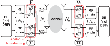
Figure 1: Both a transmitter and a receiver have $N_{RF}$ analog beamforming vectors and a baseband (BB) signal processing block including digital beamforming (DBF). This paper focuses on an analog beam selection problem, which dominates the complexity and performance of hybrid beamforming systems [10].

II System Model

A system having a transmitter with an $N_{T}$-element uniform linear antenna array (ULA) communicates $N_{RF}$ data streams to a receiver with an $N_{R}$-element ULA as shown in Fig. 1. The $N_{RF}$ analog beamforming vectors at the transmitter in matrix $\mathbf{F}=[\mathbf{f}_{1},\cdots,\mathbf{f}_{N_{RF}}]$ are selected from a predefined codebook $\mathcal{F}=\{\tilde{\mathbf{f}}_{n_{f}}\in\mathbb{C}^{N_{T}\times 1},n_{f}=1,\cdots,N_{F}\}$ with the $n_{f}^{\text{th}}$ member represented as [2]

$$\tilde{\mathbf{f}}_{n_{f}}=\frac{1}{\sqrt{N_{T}}}\left[1,e^{j\frac{2\pi}{\lambda_{0}}\text{sin}(\phi_{T,n_{f}})\Delta_{d}},\cdots,\right.\\ \left.e^{j\frac{2\pi}{\lambda_{0}}\text{sin}(\phi_{T,n_{f}})\cdot(N_{T}-1)\Delta_{d}}\right]^{T},$$ (1)

where $\phi_{T,n_{f}}$ stands for the $n_{f}^{\text{th}}$ candidate of the steering angles at the transmitter, $\Delta_{d}=\tfrac{\lambda_{0}}{2}$ is the distance between two neighboring antennas, and $\lambda_{0}$ is the wavelength at the carrier frequency. At the receiver, the $N_{RF}$ analog beamforming vectors in matrix $\mathbf{W}=[\mathbf{w}_{1},\cdots,\mathbf{w}_{N_{RF}}]$ are selected from the other codebook defined as $\mathcal{W}=\{\tilde{\mathbf{w}}_{n_{w}}\in\mathbb{C}^{N_{R}\times 1},n_{w}=1,\cdots,N_{W}\}$, where the members can be generated by the same rule as (1). The analog beamforming matrices $\mathbf{F}$ and $\mathbf{W}$ are assumed to be constant within one OFDM symbol duration owing to hardware constraints.

Via a coupling of two analog beamforming matrices and a multipath matrix-valued CIR $\mathbf{H}[l]\in\mathbb{C}^{N_{R}\times N_{T}}$, where $l=0,\cdots,L-1$ denotes the sample in one OFDM symbol, the $l^{\text{th}}$ sampled received signal vector $\mathbf{r}[l]\in\mathbb{C}^{N_{RF}\times 1}$ can be written as

$$\mathbf{r}[l] =\sqrt{\rho}\cdot\mathbf{W}^{H}\mathbf{H}[l]\circledast_{L}\mathbf{F}\mathbf{s}[l]+\mathbf{W}^{H}\mathbf{n}[l],$$ (2)

where $\rho$ stands for the average received power containing the transmit power, transmit antenna gain, receive antenna gain, and path loss, $\mathbf{s}[l]\in\mathbb{C}^{N_{RF}\times 1}$ is the transmitted signal vector, and $\mathbf{n}[l]\in\mathbb{C}^{N_{R}\times 1}$ is an $N_{R}$-dimensional independent and identically distributed (i.i.d.) complex Gaussian random vector, $\mathbf{n}[l]\sim\mathcal{CN}(\boldsymbol{0}_{N_{R}\times 1},\sigma_{n}^{2}\mathbf{I}_{N_{R}})$.

mmWave channel models have been widely studied recently [14, 15]. Based on the references, a simplified mmWave CIR matrix $\mathbf{H}[l]$ can be expressed as the sum of $P$ outer products of the array response vectors associated with the normalized-quantized delay $l_{p}=\left\lfloor\tau_{p}F_{S}\right\rfloor\in\mathbb{N}_{0}$ (the set of natural numbers contains zero), where $\tau_{p}\in\mathbb{R}_{\geq 0}$ (the set of positive real numbers contains zero) is the delay for path $p$ and $F_{S}$ is the sampling rate,

$$\mathbf{H}[l] =\sum_{p=1}^{P}\underset{c_{p}[l]}{\underbrace{\alpha_{p}\delta[l-l_{p}]}}\cdot\mathbf{a}_{A}(\phi_{A,p})\mathbf{a}_{D}(\phi_{D,p})^{H}$$ (3)

$$=\sum_{p=1}^{P}c_{p}[l]\mathbf{a}_{A}(\phi_{A,p})\mathbf{a}_{D}^{H}(\phi_{D,p})$$

where $\alpha_{p}\in\mathbb{R}_{>0}$ is the attenuation coefficient for path $p$ and $\sum_{p=1}^{P}|\alpha_{p}|^{2}=1$. Note that the path loss values influenced by an environment and geometry are mentioned in the average received power $\rho$ in (2). $c_{p}[l]$ characterizes the CIR for path $p$ at sample $l$ and we assume that $c_{p}[l]=0$ when $l\geq L_{C}$, where $L_{C}$ is the CP length. The departure array response vector $\mathbf{a}_{D}(\phi_{D,p})$ is a function of angle of departure (AoD), $\phi_{D,p}\sim\mathcal{U}(-\tfrac{\pi}{2},\tfrac{\pi}{2})$, for path $p$,

$$\mathbf{a}_{D}(\phi_{D,p})=\frac{1}{\sqrt{N_{T}}}\left[1,e^{j\tfrac{2\pi}{\lambda_{0}}\text{sin}(\phi_{D,p})\Delta_{d}},\cdots,\right.\\ \left.e^{j\tfrac{2\pi}{\lambda_{0}}\text{sin}(\phi_{D,p})(N_{T}-1)\Delta_{d}}\right]^{T},$$ (4)

and the arrival array response vector $\mathbf{a}_{A}(\phi_{A,p})$, where $\phi_{A,p}\sim\mathcal{U}(-\tfrac{\pi}{2},\tfrac{\pi}{2})$, has a similar form as (4).

III Time-Domain Analog Beam Selection

III-A Observations for analog beam selection

In order to acquire the observations for the analog beam selection, we simply assume that all the beam pairs selected from $\mathcal{F}$ and $\mathcal{W}$ are trained by a known training sequence. Hypothetically there is no data transmission and reception before the transmitter and receiver select the preferable analog beam pairs. Hence, one can use a training sequence of length $L$ in one OFDM symbol, $\{s[0],\cdots,s[L-1]\}$, to train one beam pair. The $l^{\text{th}}$ sampled scalar of the received signals by using the beam pair $(\tilde{\mathbf{f}}_{n_{f}},\tilde{\mathbf{w}}_{n_{w}})$ can therefore be expressed as

$$r_{n_{w},n_{f}}[l] =\sqrt{\rho}\cdot\tilde{\mathbf{w}}_{n_{w}}^{H}\mathbf{H}[l]\circledast_{L}\tilde{\mathbf{f}}_{n_{f}}s[l]+\underset{z_{n_{w},n_{f}}[l]}{\underbrace{\tilde{\mathbf{w}}_{n_{w}}^{H}\mathbf{n}[l]}}$$ (5)

$$=\sqrt{\rho}\cdot\tilde{\mathbf{w}}_{n_{w}}^{H}\mathbf{H}[l]\circledast_{L}\tilde{\mathbf{f}}_{n_{f}}s[l]+z_{n_{w},n_{f}}[l],$$

where $n_{f}=1,\cdots,N_{F}$, $n_{w}=1,\cdots,N_{W}$, the combined noise $z_{n_{w},n_{f}}[l]\sim\mathcal{CN}(0,\sigma_{n}^{2})$ still has a Gaussian distribution with mean zero and variance $\sigma_{n}^{2}$ due to the equal-magnitude elements of $\tilde{\mathbf{w}}_{n_{w}}$.

To implement deconvolution of the received signal and get the observations for the beam selection, we intend to decouple the angle- and delay-domain components in $r_{n_{w},n_{f}}[l]$ by replacing the channel matrix $\mathbf{H}[l]$ with (3). Consequently, $r_{n_{w},n_{f}}[l]$ can be further written as follows:

$$r_{n_{w},n_{f}}[l]$$ (6)

$$=\sqrt{\rho}\cdot\sum_{p=1}^{P}\underset{\triangleq\eta_{p,n_{w},n_{f}}}{\underbrace{\tilde{\mathbf{w}}_{n_{w}}^{H}\mathbf{a}_{A}(\phi_{A,p})\mathbf{a}_{D}^{H}(\phi_{D,p})\tilde{\mathbf{f}}_{n_{f}}}}\left(c_{p}[l]\circledast_{L}s[l]\right)+z_{n_{w},n_{f}}[l]$$

$$=\sqrt{\rho}\cdot\sum_{p=1}^{P}\eta_{p,n_{w},n_{f}}\cdot\left(c_{p}[l]\circledast_{L}s[l]\right)+z_{n_{w},n_{f}}[l],$$

where $|\eta_{p,n_{w},n_{f}}|=|\tilde{\mathbf{w}}_{n_{w}}^{H}\mathbf{a}_{A}(\phi_{A,p})|\cdot|\mathbf{a}_{D}^{H}(\phi_{D,p})\tilde{\mathbf{f}}_{n_{f}}|$ is the multiplication of beamforming gains at the transmitter and receiver.

Then, we collect $L$ samples in a vector and express the circular convolution as a multiplication by a circulant matrix $\mathbf{S}$ [16]

$$\mathbf{r}_{n_{w},n_{f}} =\left[r_{n_{w},n_{f}}[0],\cdots,r_{n_{w},n_{f}}[L-1]\right]^{T}$$ (7)

$$=\sqrt{\rho}\cdot\mathbf{S}\sum_{p=1}^{P}\eta_{p,n_{w},n_{f}}\mathbf{c}_{p}+\mathbf{z}_{n_{w},n_{f}},$$

where

$$\mathbf{S} =\left[\begin{array}[]{ccc}s[0]&\cdots&s[1]\\ \vdots&\ddots&\vdots\\ s[L-1]&\cdots&s[0]\end{array}\right]\in\mathbb{C}^{L\times L},$$ (8d)

$$\mathbf{c}_{p} =\left[c_{p}[0],\cdots,c_{p}[L-1]\right]^{T}\in\mathbb{C}^{L\times 1},$$ (8e)

$$\mathbf{z}_{n_{w},n_{f}} =\left[z_{n_{w},n_{f}}[0],\cdots,z_{n_{w},n_{f}}[L-1]\right]^{T}\in\mathbb{C}^{L\times 1}.$$ (8f)

The $L$ observations can therefore be obtained by pre-multiplying $\mathbf{r}_{n_{w},n_{f}}$ by $\mathbf{S}^{-1}$, where $\det(\mathbf{S})\neq 0$, given by

$$y_{n_{w},n_{f}}[l] =\left[\mathbf{S}^{-1}\right]_{l,:}\mathbf{r}_{n_{w},n_{f}}$$ (9)

$$=\sqrt{\rho}\cdot\sum_{p=1}^{P}\eta_{p,n_{w},n_{f}}c_{p}[l]+\underset{\xi_{n_{w},n_{f}}[l]}{\underbrace{\left[\mathbf{S}^{-1}\right]_{l,:}\mathbf{z}_{n_{w},n_{f}}}}$$

$$=\sqrt{\rho}\cdot\tilde{\mathbf{w}}_{n_{w}}^{H}\mathbf{H}[l]\tilde{\mathbf{f}}_{n_{f}}+\xi_{n_{w},n_{f}}[l],$$

where $l=0,\cdots,L-1$. One can design the training sequence so that $\xi_{n_{w},n_{f}}[l]$ has a complex Gaussian distribution with mean zero and a variance of $\sigma_{\xi}^{2}$.

III-B Problem statement

The observations $\{y_{n_{w},n_{f}}[l]\>\forall n_{w},n_{f},l\}$ can be interpreted as coupling coefficients of the channel and the trained beam pairs. If the coupling coefficients are acquired in the frequency domain, our previous work in [10] introduces how to use them to select the analog beam pairs. Simply speaking, the problem of frequency-domain analog beam selection can be formulated as finding the beam pairs that maximize the sum of the power of the observations across all subcarriers. From Parseval’s theorem, we know that the objective function is equivalent to the sum of the power across all samples in the delay domain. As a result, the delay-domain analog beam selection can be expressed as the following maximization problem:

$$\begin{gathered}(\hat{\mathbf{f}}_{n_{rf}},\hat{\mathbf{w}}_{n_{rf}})={\displaystyle\underset{\scriptsize\begin{array}[]{c}\tilde{\mathbf{f}}_{n_{f}}\in\mathcal{F}\backslash\mathcal{F}^{\prime},\tilde{\mathbf{w}}_{n_{w}}\in\mathcal{W}\backslash\mathcal{W}^{\prime}\end{array}}{\arg\,\max}}g_{n_{w},n_{f}},\end{gathered}$$ (10)

where $n_{rf}=1,\cdots,N_{RF}$, $g_{n_{w},n_{f}}$ is the energy of the observations

$$\begin{aligned} g_{n_{w},n_{f}}&=\sum_{l=0}^{L-1}\left|y_{n_{w},n_{f}}[l]\right|^{2}\end{aligned},$$ (11)

$\mathcal{F}^{\prime}=\{\hat{\mathbf{f}}_{n},n=1,\cdots,n_{rf}-1\}$ and $\mathcal{W}^{\prime}=\{\hat{\mathbf{w}}_{n},n=1,\cdots,n_{rf}-1\}$ are the sets including the selected analog beamforming vectors from iteration $1$ to $n_{rf}-1$. The energy estimate $g_{n_{w},n_{f}}$ is also the objective function used in frequency-domain analog beam selection problem [10]. However, in the frequency domain, we do not have the information that $y_{n_{w},n_{f}}[l]$, $l=L_{C},\cdots,L-1$, only contain noise signals.

In the beam selection problem stated in (10), the sum of the power of $L$ noise-free observations, i.e.,

$$y_{n_{w},n_{f}}^{N\!F}[l]\triangleq\sqrt{\rho}\,\tilde{\mathbf{w}}_{n_{w}}^{H}\mathbf{H}[l]\tilde{\mathbf{f}}_{n_{f}},$$ (12)

where $l=0,\cdots,L-1$, would lead to the optimal solution. Let us write down the corresponding objective function

$$g_{n_{w},n_{f}}^{N\!F} \triangleq\sum_{l=0}^{L-1}\left|y_{n_{w},n_{f}}^{N\!F}[l]\right|^{2}$$ (13)

$$=\sum_{p=1}^{P}\left|\sqrt{\rho}\,\tilde{\mathbf{w}}_{n_{w}}^{H}\mathbf{H}[l_{p}]\tilde{\mathbf{f}}_{n_{f}}\right|^{2},$$

where the second equality follows from that $\mathbf{H}[l]=0$ when $l\notin\{l_{p},p=1,\cdots,P\}$ and $l_{p}$, $p=1,\cdots,P$, are different to each other. Compared with (11), it is clear that in (13) only $P$ (rather than $L$) observations associated with the $P$ delay indices have to be taken into account. Therefore, our goal is to reduce the error between the energy estimate $g_{n_{w},n_{f}}$ and its true value $g_{n_{w},n_{f}}^{N\!F}$ without an additional computational overhead.

IV Performance Improvement of Analog Beam Selection in Time Domain

IV-A Performance metric

From the discussion in the previous subsection, we know that there is a higher probability to find the optimal solution when the error between $g_{n_{w},n_{f}}$ and $g_{n_{w},n_{f}}^{N\!F}$ approximates to zero. Therefore, we use the MAE between $g_{n_{w},n_{f}}$ and $g_{n_{w},n_{f}}^{N\!F}$ as a performance metric to quantify the performance of beam selection, which is stated in Theorem 1. We consider the MAE rather than the mean squared error (MSE) due to that fact that $g_{n_{w},n_{f}}$ and $g_{n_{w},n_{f}}^{N\!F}$ are energy signals; it is redundant to calculate the squared error between these two values.

Theorem 1.

Given matrix-valued CIRs $\underline{\mathbf{H}}[l]$, $l=0,\cdots,L-1$, one has the energy estimates

$$\underline{g}_{n_{w},n_{f}}=\sum_{l=0}^{L-1}\left|\sqrt{\rho}\,\tilde{\mathbf{w}}_{n_{w}}^{H}\underline{\mathbf{H}}[l]\tilde{\mathbf{f}}_{n_{f}}+\xi_{n_{w},n_{f}}[l]\right|^{2}\,\forall n_{w},n_{f}$$ (14)

and the corresponding true values

$$\underline{g}_{n_{w},n_{f}}^{N\!F}=\sum_{p=1}^{P}\left|\sqrt{\rho}\,\tilde{\mathbf{w}}_{n_{w}}^{H}\underline{\mathbf{H}}[l_{p}]\tilde{\mathbf{f}}_{n_{f}}\right|^{2}\,\forall n_{w},n_{f}.$$ (15)

Then the MAE between $\underline{g}_{n_{w},n_{f}}$ and $\underline{g}_{n_{w},n_{f}}^{N\!F}$ is upper bounded by

$$\text{MAE}(\underline{g}_{n_{w},n_{f}}) \triangleq\text{E}\left[\left|\underline{g}_{n_{w},n_{f}}-\underline{g}_{n_{w},n_{f}}^{N\!F}\right|\right]$$ (16)

$$\leq\text{E}\left[\left|\varepsilon_{n_{w},n_{f}}\right|\right]+\text{E}\left[\nu\right],$$

where

$$\varepsilon_{n_{w},n_{f}}\sim\mathcal{N}\left(0,2\sigma_{\xi}^{2}\underline{g}_{n_{w},n_{f}}^{N\!F}\right)$$ (17)

and

$$\nu\sim\Gamma(L,\sigma_{\xi}^{2}).$$ (18)

Proof:

See Appendix A. ∎

IV-B Refine observations by averaging random noise signals

In OFDM systems, the CP length ($L_{C}$) is designed to cover the maximum or root-mean-square (RMS) delay spread, which means that the number of useful observations in one OFDM symbol is less than or equal to $L_{C}$. To improve the quality of the observations, we use a property of circular convolutions introduced as follows. First, simply modifying the transmitted training sequence of length $L$ as $M=\tfrac{L}{L_{C}}$ (assume $\tfrac{L}{L_{C}}\in\mathbb{N}^{+}$) repeated sequence blocks, where the length of each block is $L_{C}$. Such periodic training sequence blocks make the circular convolution in (6) become

$$c_{p}[l]\circledast_{L}s[l] =\sum_{n=0}^{L-1}c_{p}[n]s[l-n]$$ (19)

$$=\sum_{n=0}^{L_{C}-1}c_{p}[n]s[l-n]$$

$$=c_{p}[l]\circledast_{L_{C}}s[l],$$

where the second equality follows from that $c_{p}[l]=0$ when $l\geq L_{C}$, and $\circledast_{L_{C}}$ denotes a circular convolution over the cyclic group of integers modulo $L_{C}$. Then, following from (9), we can use a circulant matrix of small size $L_{C}\times L_{C}$ (generated by one training sequence block) to sequentially implement the deconvolution of $M$ received periodic blocks. An arithmetic mean of the $M$ outputs of the deconvolution leads to a result suffering from less noise effect

$$y_{n_{w},n_{f}}^{\prime}[l_{c}] =y_{n_{w},n_{f}}^{N\!F}[l_{c}]+\underset{\xi_{n_{w},n_{f}}^{\prime}[l_{c}]}{\underbrace{\frac{1}{M}\sum_{m=1}^{M}\xi_{n_{w},n_{f}}[(m-1)L_{C}+l_{c}]}}$$ (20)

$$=y_{n_{w},n_{f}}^{N\!F}[l_{c}]+\xi_{n_{w},n_{f}}^{\prime}[l_{c}],$$

where $l_{c}=0,\cdots,L_{C}-1$, and the variance of $\xi_{n_{w},n_{f}}^{\prime}[l_{c}]\sim\mathcal{CN}\left(0,\frac{\sigma_{\xi}^{2}}{M}\right)$ is effectively reduced by a factor of $M$. By using these averaged (or refined) observations, the energy estimate in (11) becomes

$$g_{n_{w},n_{f}}^{\prime}=\sum_{l_{c}=0}^{L_{C}-1}\left|y_{n_{w},n_{f}}^{\prime}[l_{c}]\right|^{2}.$$ (21)

Based on the derivation of Theorem 1, the MAE between the estimate $g_{n_{w},n_{f}}^{\prime}$ and its true value $g_{n_{w},n_{f}}^{N\!F}$ conditioned on the same channel realizations, $\underline{\mathbf{H}}[l]$, $l=0,\cdots,L-1$, is given by

$$\text{MAE}\left(\underline{g}_{n_{w},n_{f}}^{\prime}\right) \triangleq\text{E}\left[\left|\underline{g}_{n_{w},n_{f}}^{\prime}-\underline{g}_{n_{w},n_{f}}^{N\!F}\right|\right]$$ (22)

$$\leq\text{E}\left[\left|\varepsilon_{n_{w},n_{f}}^{\prime}\right|\right]+\text{E}\left[\nu^{\prime}\right],$$

where $\varepsilon_{n_{w},n_{f}}^{\prime}$ has a Gaussian distribution

$$\varepsilon_{n_{w},n_{f}}^{\prime}\sim\mathcal{N}\left(0,2\left(\frac{\sigma_{\xi}^{2}}{M}\right)\underline{g}_{n_{w},n_{f}}^{N\!F}\right),$$ (23)

and $\nu^{\prime}$ follows a gamma distribution

$$\nu^{\prime}\sim\Gamma\left(\frac{L}{M},\frac{\sigma_{\xi}^{2}}{M}\right).$$ (24)

Compared with (17), (18), the noise effect caused by $\varepsilon_{n_{w},n_{f}}^{\prime}$ and $\nu^{\prime}$ can be effectively reduced when $M$ is large. For example, one of the use cases in 3GPP 5G NR [13] shows that the CP ratio $\tfrac{1}{M}\approx\tfrac{1}{14}$.

IV-C Further refine observations by using knowledge of multipath delay

In the previous subsection, we present how to enhance the quality of the observations. Without any information of multipath delay, the $L_{C}$ signals in (20), $\{y_{n_{w},n_{f}}^{\prime}[l_{c}],\,l_{c}=0,\cdots,L_{C}-1\}$, with respect to a certain beam pair $(\tilde{\mathbf{f}}_{n_{f}},\tilde{\mathbf{w}}_{n_{w}})$ are regarded as useful observations. Nevertheless, only $P$ sparse observations corresponding to the $P$ CIRs are exactly useful. Fortunately, we can borrow the idea of the analog beam selection in (10) to find the multipath delay indices because the signals $\{y_{n_{w},n_{f}}^{\prime}[l_{c}],\,\forall n_{w},n_{f},l_{c}\}$ are represented in the discrete delay-angle domain, where $l_{c}$ and $(n_{w},n_{f})$ respectively denote the delay- and angle-domain indices. Accordingly, the multipath delay estimation can be stated as the following problem: given $\{y_{n_{w},n_{f}}^{\prime}[l_{c}],\,\forall n_{w},n_{f},l_{c}\}$, one can calculate the sum of the power of $N_{W}N_{F}$ observations across all steering angles as

$$\begin{aligned} f[l_{c}]&=\sum_{n_{w}=1}^{N_{W}}\sum_{n_{f}=1}^{N_{F}}\left|y_{n_{w},n_{f}}^{\prime}[l_{c}]\right|^{2}\end{aligned},$$ (25)

and solve the constrained maximization problem

$$\begin{gathered}\hat{l}_{\hat{p}}={\displaystyle\underset{\tiny l_{c}\in\{0,\cdots,L_{C}-1\}\backslash\mathcal{L}}{\arg\text{ }\max}}f[l_{c}],\\ \text{s.t. }\begin{cases}f[l_{c}]\geq\mu,\\ \mathcal{L}=\{\hat{l}_{n},n=1,\cdots,\hat{p}-1\},\end{cases}\end{gathered}$$ (26)

where $\hat{p}=1,\cdots,\hat{P}$ denotes the path index whose received power across all steering angles is greater than or equal to a pre-defined threshold $\mu$, and $\mathcal{L}$ is the set containing the selected path indices from iteration $1$ to $\hat{p}-1$. Here we consider the sum of the power of $N_{W}N_{F}$ observations in the angle domain; therefore the threshold can be simply assumed to be $\mu=N_{W}N_{F}\left(\frac{\sigma_{\xi}^{2}}{M}\right)$. Since mmWave channels are sparse in nature, the multipath delay indices can be estimated by using this characteristic to further improve the performance [17]. Due to the page limit, we do not provide more discussion.

According to the estimated delay indices, only $\hat{P}$ refined observations are used for the analog beam selection problem (assume $P\leq\hat{P}<L_{C}$ but $\{\hat{l}_{\hat{p}}\;\forall\hat{p}\}$ does not necessarily include $\{l_{p}\>\forall p\}$) and the corresponding objective function is given by

$$\begin{aligned} g_{n_{w},n_{f}}^{\prime\prime}&=\sum_{\hat{p}=1}^{\hat{P}}\left|y_{n_{w},n_{f}}^{\prime}[\hat{l}_{\hat{p}}]\right|^{2}\end{aligned}.$$ (27)

Similarly, conditioned on the same channel realizations, $\underline{\mathbf{H}}[l]$, $l=0,\cdots,L-1$, we have the MAE between $g_{n_{w},n_{f}}^{\prime\prime}$ and its true value $g_{n_{w},n_{f}}^{N\!F}$ upper bounded by

$$\text{MAE}(\underline{g}_{n_{w},n_{f}}^{\prime\prime}) \triangleq\text{E}\left[\left|\underline{g}_{n_{w},n_{f}}^{\prime\prime}-\underline{g}_{n_{w},n_{f}}^{N\!F}\right|\right]$$ (28)

$$\leq\underline{g}_{n_{w},n_{f}}^{N\!F}-\underline{g}_{n_{w},n_{f}}^{\prime\prime N\!F}+\text{E}\left[\left|\varepsilon_{n_{w},n_{f}}^{\prime\prime}\right|\right]+\text{E}\left[\nu^{\prime\prime}\right],$$

where

$$\underline{g}_{n_{w},n_{f}}^{\prime\prime N\!F}=\sum_{\hat{p}=1}^{\hat{P}}\left|\underline{y}_{n_{w},n_{f}}^{N\!F}[\hat{l}_{\hat{p}}]\right|^{2}$$ (29)

and $\underline{g}_{n_{w},n_{f}}^{\prime\prime N\!F}\leq\underline{g}_{n_{w},n_{f}}^{N\!F}$ with equality iff $\{\hat{l}_{\hat{p}}\>\forall\hat{p}\}\supseteq\{l_{p}\>\forall p\}$. Furthermore, $\varepsilon_{n_{w},n_{f}}^{\prime\prime}$ and $\nu^{\prime\prime}$ are given as follows:

$$\varepsilon_{n_{w},n_{f}}^{\prime\prime}\sim\mathcal{N}\left(0,2\left(\frac{\sigma_{\xi}^{2}}{M}\right)\underline{g}_{n_{w},n_{f}}^{\prime\prime N\!F}\right)$$ (30)

and

$$\nu^{\prime\prime}\sim\Gamma\left(\hat{P},\frac{\sigma_{\xi}^{2}}{M}\right).$$ (31)

Compared with $\varepsilon_{n_{w},n_{f}}^{\prime}$ and $\nu^{\prime}$, although the variance of $\varepsilon_{n_{w},n_{f}}^{\prime\prime}$ and the shape parameter of $\nu^{\prime\prime}$ become smaller, $\text{MAE}(\underline{g}_{n_{w},n_{f}}^{\prime\prime})$ is not necessarily less than $\text{MAE}(\underline{g}_{n_{w},n_{f}}^{\prime})$ if the difference between $\underline{g}_{n_{w},n_{f}}^{N\!F}$ and $\underline{g}_{n_{w},n_{f}}^{\prime\prime N\!F}$ is too large. It depends on the performance of multipath delay estimation.

V Numerical Results

The system parameters used in the simulations are listed below:
Number of antennas $N_{T}=N_{R}=32$ Number of RF chains $N_{RF}=2$ Number of samples per OFDM symbol $L=2048$ CP length $L_{C}=128$ Codebook size $N_{F}=N_{W}=32$ Number of paths $P=10$
In addition, the effective noise variance is given by $\sigma_{\xi}^{2}=\rho\cdot 10^{-\gamma/10}$, where $\gamma$ (dB) is the SNR. In the codebooks, $32$ steering angle candidates are: $\left\{\frac{180^{\circ}}{\pi}\cdot\sin^{-1}\left(\frac{\left(n_{f}-16\right)}{16}\right),\,n_{f}=1,\cdots,32\right\}$ [18].

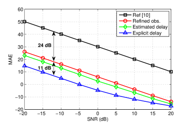
Figure 2: MAE between energy estimates and their true value, where Ref uses $L=2048$ unrefined observations, and others use $L_{C}=128$ refined observations with and without knowledge of multipath delay.

As discussed in Section III-B, the true value of the energy yields the optimal solution of the problem in (10). Let us denote the indices of the optimal beam pairs as $(\mathring{n}_{w,n_{r\!f}},\mathring{n}_{f,n_{r\!f}})\>\forall n_{r\!f}$, and then use the MAE as a performance metric to evaluate the performance of the proposed and reference methods with respect to the beam pairs $(\mathring{n}_{w,n_{r\!f}},\mathring{n}_{f,n_{r\!f}})\>\forall n_{r\!f}$. In Fig. 2, the curves labeled as Ref, Refined obs., and Estimated delay are respectively calculated by the following equations:

Ref $$=\frac{1}{N_{RF}}\sum_{n_{r\!f}=1}^{N_{RF}}\text{MAE}(g_{\mathring{n}_{w,n_{r\!f}},\mathring{n}_{f,n_{r\!f}}}),$$ (32a)

Refined obs. $$=\frac{1}{N_{RF}}\sum_{n_{r\!f}=1}^{N_{RF}}\text{MAE}(g_{\mathring{n}_{w,n_{r\!f}},\mathring{n}_{f,n_{r\!f}}}^{\prime}),$$ (32b)

Estimated delay $$=\frac{1}{N_{RF}}\sum_{n_{r\!f}=1}^{N_{RF}}\text{MAE}(g_{\mathring{n}_{w,n_{r\!f}},\mathring{n}_{f,n_{r\!f}}}^{\prime\prime}),$$ (32c)

where the energy estimate in (32a) is equivalent to the sum of the power of observations across all subcarriers, which is the objective function of the frequency-domain analog beam selection problem in [10].

From (16) and (22), we can find the upper bounds of (32a) and (32b), and they are dominated by the gamma distributed random variables when the values of shape and scale parameters are large. As a result, (32a) and (32b) can be approximated by

$$(\ref{eq: MAE1}) \approx\text{E}\left[\nu\right],$$ (33a)

$$(\ref{eq: MAE2}) \approx\text{E}\left[\nu^{\prime}\right].$$ (33b)

and therefore the difference in MAE between Ref and Refined obs. is given by

$$10\log_{10}\left(\frac{\text{E}\left[\nu\right]}{\text{E}\left[\nu^{\prime}\right]}\right)=10\log_{10}\left(M^{2}\right)=24.08\,\text{dB}.$$

In (32c), if we only use $\hat{P}$ refined observations associated with $\hat{P}$ estimated delay indices (the estimation error rate is shown in Fig. 3), the MAE can be reduced by $3$ dB compared with Refined obs., see curve Estimated delay. Ideally, if the set containing $\hat{P}$ estimated delay indices is equal to $\{l_{p}\>\forall p\}$, following from (28), the corresponding MAE is upper bounded by

$$\text{MAE}(\underline{g}_{n_{w},n_{f}}^{\prime\prime}|_{\text{given }\{l_{p}\,\forall p\}})$$ (34)

$$\leq\text{E}\left[\left|\varepsilon_{n_{w},n_{f}}^{\prime\prime}|_{\text{given }\{l_{p}\,\forall p\}}\right|\right]+\text{E}\left[\nu^{\prime\prime}|_{\text{given }\{l_{p}\,\forall p\}}\right]$$

$$=\text{E}\left[\left|\varepsilon_{n_{w},n_{f}}^{\prime}\right|\right]+\text{E}\left[\nu^{\prime\prime}|_{\text{given }\{l_{p}\,\forall p\}}\right]$$

where

$$\nu^{\prime\prime}|_{\text{given }\{l_{p}\,\forall p\}}\sim\Gamma\left(P,\frac{\sigma_{\xi}^{2}}{M}\right),$$ (35)

and the simulation results are shown in curve Explicit delay calculated by

$$\text{Explicit delay}=\frac{1}{N_{RF}}\sum_{n_{r\!f}=1}^{N_{RF}}\text{MAE}(\underline{g}_{\mathring{n}_{w,n_{r\!f}},\mathring{n}_{f,n_{r\!f}}}^{\prime\prime}|_{\text{given }\{l_{p}\,\forall p\}}).$$ (36)

In the low SNR regime, $\text{MAE}(\underline{g}_{n_{w},n_{f}}^{\prime\prime}|_{\text{given }\{l_{p}\,\forall p\}})$ is dominated by the gamma distributed random variable as well. Hence, the difference in MAE between Refined obs. and Explicit delay approximates to

$$10\log_{10}\left(\frac{\text{E}\left[\nu^{\prime}\right]}{\text{E}\left[\nu^{\prime\prime}|_{\text{given }\{l_{p}\,\forall p\}}\right]}\right)=10\log_{10}\left(\frac{L}{MP}\right)=11.07\,\text{dB}.$$ (37)

When the SNR increases, (36) is not only dominated by the gamma distributed random variable, so the difference between Refined obs. and Explicit delay cannot be simply approximated by (37).

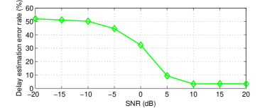
Figure 3: Estimation error rate of $P$ delay indices in curve Estimated delay in Fig. 2.

In Fig. 3, it shows the estimation error rate of $P$ delay indices in curve Estimated delay in Fig. 2. As mentioned in Section IV-C, since the exact number $P=10$ of paths is not available, we try to find $\hat{P}$ paths whose sum of the received power across all steering angles are greater than or equal to the pre-defined threshold $\mu=\left(\frac{\sigma_{\xi}^{2}}{M}\right)N_{W}N_{F}$. When $\text{SNR}<0\text{ dB}$, the delay estimation error rate of more than $30\%$ leads to an MAE reduction of approximately $3$ dB, compared with Refined obs. On the other hand, when $\text{SNR}\geq 10\text{ dB}$, the delay estimation error rate approximates to zero. However, the gap between Estimated delay and Explicit delay in Fig. 2 is still quite obvious, which means that $\hat{P}\gg P$ and therefore not only the useful observations but also a large number of noise signals are reserved. The delay estimation approach can be further enhanced by, for example, modifying the threshold; nevertheless, it is beyond the scope of this paper.

$$\underline{g}_{n_{w},n_{f}} =\sum_{l=0}^{L-1}\left|\sqrt{\rho}\,\tilde{\mathbf{w}}_{n_{w}}^{H}\underline{\mathbf{H}}[l]\tilde{\mathbf{f}}_{n_{f}}+\xi_{n_{w},n_{f}}[l]\right|^{2}$$ (38)

$$=\sum_{l=0}^{L-1}\left|\underline{y}_{n_{w},n_{f}}^{N\!F}[l]+\xi_{n_{w},n_{f}}[l]\right|^{2}$$

$$=\sum_{l=0}^{L-1}\mathfrak{R}\left(\underline{y}_{n_{w},n_{f}}^{N\!F}[l]+\xi_{n_{w},n_{f}}[l]\right)^{2}+\mathfrak{I}\left(\underline{y}_{n_{w},n_{f}}^{N\!F}[l]+\xi_{n_{w},n_{f}}[l]\right)^{2}$$

$$=\underset{\triangleq\underline{g}_{n_{w},n_{f}}^{N\!F}}{\underbrace{\sum_{l=0}^{L-1}\mathfrak{R}\left(\underline{y}_{n_{w},n_{f}}^{N\!F}[l]\right)^{2}+\mathfrak{I}\left(\underline{y}_{n_{w},n_{f}}^{N\!F}[l]\right)^{2}}}+\underset{\triangleq\varepsilon_{n_{w},n_{f}}}{\underbrace{\sum_{l=0}^{L-1}2\mathfrak{R}\left(\underline{y}_{n_{w},n_{f}}^{N\!F}[l]\right)\mathfrak{R}\left(\xi_{n_{w},n_{f}}[l]\right)+2\mathfrak{I}\left(\underline{y}_{n_{w},n_{f}}^{N\!F}[l]\right)\mathfrak{I}\left(\xi_{n_{w},n_{f}}[l]\right)}}$$

$$\quad\,+\underset{\triangleq\nu}{\underbrace{\sum_{l=0}^{L-1}\mathfrak{R}\left(\xi_{n_{w},n_{f}}[l]\right)^{2}+\mathfrak{I}\left(\xi_{n_{w},n_{f}}[l]\right)^{2}}}$$

$$=\underline{g}_{n_{w},n_{f}}^{N\!F}+\varepsilon_{n_{w},n_{f}}+\nu,$$

VI Conclusion

The mmWave channel sparsity in the delay domain is widely acknowledged as a powerful cue for analog beam selection. Different to the conventional methods addressing the feature in the frequency domain, this paper presents a new perspective in the delay domain and shows that the significant observations used for the analog beam selection are also sparse. To improve the quality of the observations, we propose a solution that transmits the periodic training sequence of length equal to a CP length. An arithmetic mean can accordingly reduce the noise variance to refine the observations. Then based on the refined signals represented in the delay-angle domain, the sparse significant observations can be simply captured by finding the maximum term in the sum of the power of the refined signals across angle.

VII Appendix

VII-A Proof of Theorem 1

Given channel matrices $\underline{\mathbf{H}}[l]$, $l=0,\cdots,L-1$, the objective function $g_{n_{w},n_{f}}$ in (11) becomes (38), where the first term $\underline{g}_{n_{w},n_{f}}^{N\!F}$ is a constant, the second term $\varepsilon_{n_{w},n_{f}}$ has a normal distribution with mean zero and variance $2\sigma_{\xi}^{2}\underline{g}_{n_{w},n_{f}}^{N\!F}$, $\varepsilon_{n_{w},n_{f}}\sim\mathcal{N}(0,2\sigma_{\xi}^{2}\underline{g}_{n_{w},n_{f}}^{N\!F})$, and the third term $\nu$ has a gamma distribution with the shape parameter $L$ and scale parameter $\sigma_{\xi}^{2}$, $\nu\sim\Gamma(L,\sigma_{\xi}^{2})$. Therefore, the MAE between $\underline{g}_{n_{w},n_{f}}$ and $\underline{g}_{n_{w},n_{f}}^{N\!F}$ (denoted as $\text{MAE}(\underline{g}_{n_{w},n_{f}})$) is given by

$$\text{MAE}(\underline{g}_{n_{w},n_{f}}) \triangleq\text{E}\left[\left|\underline{g}_{n_{w},n_{f}}-\underline{g}_{n_{w},n_{f}}^{N\!F}\right|\right]$$

$$=\text{E}\left[\left|\underline{g}_{n_{w},n_{f}}^{N\!F}+\varepsilon_{n_{w},n_{f}}+\nu-\underline{g}_{n_{w},n_{f}}^{N\!F}\right|\right]$$

$$=\text{E}\left[\left|\varepsilon_{n_{w},n_{f}}+\nu\right|\right]$$

$$\leq\text{E}\left[\left|\varepsilon_{n_{w},n_{f}}\right|\right]+\text{E}\left[\nu\right].$$

References

- [1] T. Rappaport, R. Heath, R. Daniels, and J. Murdock, Millimeter Wave Wireless Communications. Prentice Hall, 2014.
- [2] J. Liberti and T. Rappaport, Smart antennas for wireless communications: IS-95 and third generation CDMA applications. Prentice Hall, 1999.
- [3] A. Hajimiri, H. Hashemi, A. Natarajan, X. Guan, and A. Komijani, “Integrated phased array systems in silicon,” Proc. IEEE, vol. 93, no. 9, pp. 1637–1655, Sep. 2005.
- [4] B. van Veen and K. M. Buckley, “Beamforming: A versatile approach to spatial filtering,” IEEE ASSP Magazine, vol. 5, pp. 4–24, Apr. 1988.
- [5] X. Zhang, A. F. Molisch, and S.-Y. Kung, “Variable-phase-shift-based RF-baseband codesign for MIMO antenna selection,” IEEE Trans. Signal Process., vol. 53, no. 11, pp. 4091–4103, Nov. 2005.
- [6] O. E. Ayach, S. Rajagopal, S. Abu-Surra, Z. Pi, and R. W. Heath, “Spatially sparse precoding in millimeter wave MIMO systems,” IEEE Trans. Wireless Commun., vol. 13, no. 3, pp. 1499–1513, Mar. 2014.
- [7] C. H. Yu, M. P. Chang, and J. C. Guey, “Beam space selection for high rank millimeter wave communication,” in IEEE Veh. Technol. Conf. (VTC Spring), Glasgow, UK, May 2015, pp. 1–5.
- [8] S. Han, C. l. I, Z. Xu, and C. Rowell, “Large-scale antenna systems with hybrid analog and digital beamforming for millimeter wave 5G,” IEEE Commun. Mag., vol. 53, no. 1, pp. 186–194, Jan. 2015.
- [9] H. L. Chiang, W. Rave, T. Kadur, and G. Fettweis, “Hybrid beamforming based on implicit channel state information for millimeter wave links,” Sep. 2017. [Online]. Available: https://arxiv.org/abs/1709.07273
- [10] ——, “Frequency-selective hybrid beamforming based on implicit CSI for millimeter wave systems,” in IEEE Int. Conf. on Commun. (ICC), Kansas City, MO, USA, May 2018.
- [11] A. Alkhateeb and R. W. Heath, “Frequency selective hybrid precoding for limited feedback millimeter wave systems,” IEEE Trans. Commun., vol. 64, no. 5, pp. 1801–1818, May 2016.
- [12] D. Tse and P. Viswanath, Fundamentals of Wireless Communication. Cambridge University Press, 2005.
- [13] 3GPP TS 38.211 V1.0.0, “Physical channels and modulation (Release 15),” Tech. Rep., 2017.
- [14] 3GPP TR 38.900 V14.3.1, “Study on channel model for frequency spectrum above 6 GHz (Release 14),” Tech. Rep., 2017.
- [15] T. S. Rappaport, G. R. MacCartney, M. K. Samimi, and S. Sun, “Wideband millimeter-wave propagation measurements and channel models for future wireless communication system design,” IEEE Trans. Commun., vol. 63, no. 9, pp. 3029–3056, Sep. 2015.
- [16] S. M. Kay, Fundamentals of Statistical Signal Processing: Estimation Theory. Prentice Hall, 1997.
- [17] G. Gui, Q. Wan, W. Peng, and F. Adachi, “Sparse multipath channel estimation using compressive sampling matching pursuit algorithm,” in IEEE VTS Asia Pacific Wireless Commun. Symp. (APWCS), Kaohsiung, Taiwan, May 2010, pp. 10–14.
- [18] H. L. Chiang, T. Kadur, and G. Fettweis, “Analyses of orthogonal and non-orthogonal steering vectors at millimeter wave systems,” in IEEE Int. Symp. on A World of Wireless, Mobile and Multimedia Networks (WoWMoM), Coimbra, Portugal, Jun. 2016, pp. 1–6.