Coupling of magnetic order and charge transport in the candidate Dirac semimetal EuCd₂As₂

Abstract

We use resonant elastic x-ray scattering to determine the evolution of magnetic order in EuCd₂As₂ below $T_{\textrm{N}}=9.5$ K, as a function of temperature and applied magnetic field. We find an A-type antiferromagneticstructure with in-plane magnetic moments, and observe dramatic magnetoresistive effects associated with field-induced changes in the magnetic structure and domain populations. Our ab initio electronic structure calculations indicate that the Dirac dispersion found in the nonmagnetic Dirac semimetal Cd₃As₂ is also present in EuCd₂As₂, but is gapped for $T<T_{\textrm{N}}$ due to the breaking of $C_{3}$ symmetry by the magnetic structure.

I I. Introduction

The layered intermetallic EuCd₂As₂ is of interest owing to its structural relation to Cd₃As₂, the first identified example of a bulk Dirac semimetal Liu et al. (2014a); Neupane et al. (2014). It features similar networks of edge-sharing CdAs₄ tetrahedra, but in a layered rather than three-dimensional geometry and with interleaved planes of magnetic Eu²⁺ ions. While ever more non-magnetic topological phases are being proposed and discovered, the search for materials that combine non-trivial electronic topology with strong correlations has advanced at a slower pace Bansil et al. (2016); Armitage et al. (2018). Magnetism may provide a handle with which to control the unusual transport properties of Dirac fermions, such as giant negative magnetoresistance Li et al. (2016); Wang et al. (2013). This could be a first step towards an application in electronic devices Šmejkal et al. (2017).

EuCd₂As₂ was first synthesized (in polycrystalline form) in the search for novel pnictide Zintl phases by Artmann et al. Artmann et al. (1996). Pnictides with 122 stoichiometry and trigonal CaAl₂Si₂-type structure (space group $P\bar{3}m1$) are less common than related tetragonal materials, such as the superconductor parent-compound EuFe₂As₂Artmann et al. (1996); Ren et al. (2008); Paramanik et al. (2014). A number of such trigonal compounds, related to EuCd₂As₂ by ionic substitutions on any site, have recently attracted interest due to their (high temperature) thermoelectric properties Guo et al. (2013); Min et al. (2015). As in other Eu-based materials of this family Jiang and Kauzlarich (2006); Goryunov et al. (2012); Zhang et al. (2010a), low temperature magnetometry of EuCd₂As₂ powders revealed ferromagnetic correlations (a positive Curie–Weiss temperature $\Theta_{\text{CW}}=9.3\,$K) and a large effective magnetic moment of $\mu_{\textrm{eff}}=7.7\,\mu_{\text{B}}$, close to the free-ion value of $7.94\,\mu_{\text{B}}$ expected for the divalent state of Eu ($S=7/2$, $L=0$) [Artmann et al., 1996].

The unusual magnetic transition at low temperatures was initially interpreted as a successive ferromagnetic (16 K) and then antiferromagnetic (9.5 K) ordering of the Eu spins in the triangular layers. In a Mössbauer study of single-crystalline EuCd₂As₂, a ferromagnetic phase was later ruled out and attributed to Eu³⁺-containing impurities introduced by oxidation of the polycrystalline samplesSchellenberg et al. (2011).

A first investigation of EuCd₂As₂ single crystals was recently reported by Wang et al., who observed a strong coupling between charge transport and magnetic degrees of freedomWang et al. (2016a). This is seen as a strong resistivity anomaly associated with the magnetic ordering transition, which can be suppressed by an applied magnetic field.

In order to better understand the interplay between charge transport and magnetism, we have performed an in-depth resonant elastic x-ray scattering (REXS) study of the magnetic order in EuCd₂As₂, as a function of temperature and applied magnetic field. We then used these results to investigate what effect magnetic order has on the electronic structure as calculated by density functional theory.

Our REXS study establishes that EuCd₂As₂ orders into an A-type antiferromagnetic structure below $T_{\textrm{N}}=9.5$ K, with the Eu spins aligned parallel to the triangular layers. This magnetic structure breaks the $C_{3}$ symmetry of the paramagnetic phase and, according to our ab initio electronic structure calculations, opens a gap at the Dirac points in the vicinity of the Fermi surface. Conversely, these results imply that other materials of the CaAl₂Si₂–type structure could host Dirac fermions that couple to a magnetically ordered state at zero field, if the three-fold rotational symmetry is conserved.

II II. Experimental and Computational details

Single crystals of EuCd₂As₂ were synthesized by the NaCl/KCl flux growth method, as described by Schellenberg et al. Schellenberg et al. (2011). This yields shiny metallic platelets ($c$ axis surface normal) with dimensions up to $2\times 2\,\text{mm}^{2}$ and $0.5\,\text{mm}$ thickness. The samples were screened by Mo $K_{\alpha}$ x-ray diffraction Agilent Technologies XRD Products to confirm the trigonal crystal structure (space group $P\bar{3}m1$) that had been originally determined by Artmann et al. Artmann et al. (1996) (see Supplemental Material sup ; Rodriguez-Carvajal (1993)). The structure, along with the model of the zero-field magnetic order determined here, is illustrated in Fig. 1.

Measurements of the magnetic properties of EuCd₂As₂ had previously been reported for polycrystalline samples Artmann et al. (1996), and on single crystals with the field applied along an arbitrary direction Schellenberg et al. (2011). Here, we supplement these results with magnetometry data recorded in magnetic fields applied both parallel and perpendicular to the trigonal $c$ axis. These measurements were made with a superconducting quantum interference device (SQUID) magnetometer (Quantum Design Quantum Design, Inc., 10307 Pacific Center Court, San Diego, CA 92121, USA ).

The thermal variation of the resistivity of EuCd₂As₂ single crystals has recently been reported by Wang et al. Wang et al. (2016a) (at zero field and 9 T). In order to characterize the electronic transport properties of EuCd₂As₂ in more detail, we performed alternating current transport (ACT) measurements using the six-point sample contacting geometry (Quantum Design PPMS; the experimental arrangement is described in the Supplemental Material sup ). The magnetic field was applied along the $c$ axis throughout, and the current was applied in the $a$-$b$ plane.

In order to determine the magnetic structure of EuCd₂As₂, REXS experiments were performed in the second experimental hutch (EH2) of beamline P09 of PETRA-III at DESY; see Ref. Strempfer et al., 2013. Neutron diffraction studies had been called for in the literature Wang et al. (2016a), but are hindered by the extremely large neutron absorption cross-sections of both Eu (4530 b) and Cd (2520 b). On the other hand, the magnetic moments of rare earth ions are known to couple strongly to $L$ edge resonant dipole ($2p\,\rightarrow\,5d$) transitions. REXS in the hard x-ray regime, therefore, is an ideal alternative for magnetic structure determination in this material.

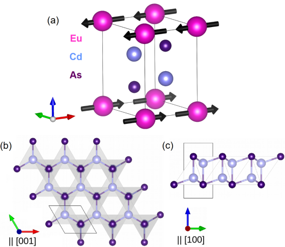
Figure 1: (a) Structural unit cell of EuCd₂As₂ with $P\bar{3}m1$ trigonal symmetry and lattice parameters $a\simeq 4.44$ Å and $c\simeq 7.33$ Å. The magnetic Eu ion is located at the origin (Wyckoff position 1a), while Cd and As atoms at 2d positions $(\nicefrac{{1}}{{3}},\nicefrac{{2}}{{3}},z_{\textrm{Cd}})$, $z_{\textrm{Cd}}\simeq 0.63$, and $(\nicefrac{{1}}{{3}},\nicefrac{{2}}{{3}},z_{\textrm{As}})$, $z_{\textrm{As}}\simeq 0.25$, form layers of Cd–As tetrahedra as illustrated in panels (b)–(c). The A-type antiferromagnetic structure, propagation vector $\mathbf{q}_{\text{m}}=(0,0,0.5)$, with in-plane magnetic moments is also shown.

Two separate EuCd₂As₂ single crystals were probed, with a magnetic field applied perpendicular and nearly parallel to the $c$ axis, respectively. To enhance the magnetic x-ray scattering from Eu²⁺ magnetic ions, the photon energy was tuned to the Eu $L_{3}$ edge at $\hbar\omega\approx 6.972\,$ keV ($\lambda=1.778\,$Å). The REXS setup at beamline P09-EH2 has several unique advantages for the present study, including a double phase retarder for full linear polarization analysis (FLPA) at hard x-ray energies and a vertical 14 T cryomagnet. We provide detailed information on the sample orientation, scattering geometry Detlefs et al. (2012); Busing and Levy (1967) and FLPA technique Mazzoli et al. (2007); Johnson et al. (2008); Hatton et al. (2009); Shukla et al. (2012); Francoual et al. (2015) in the Supplemental Material sup .

For full polarization analysis, two magnetic Bragg peaks were selected in each experimental setting. In the first setting ($\bf{H}\perp\bf{c}$), magnetic scattering at the wave vectors $(0,0,4.5)$ and $(1,0,5.5)$ (in reciprocal lattice units) was characterized in zero field as well as in applied fields of 50 and 300 mT. In the second setting ($\bf{H}\parallel\bf{c}$) we investigated peaks at $(4,0,-0.5)$ and $(4,-2,-0.5)$, in zero field and in applied fields of 0.5 and 1.0 T.

The REXS scattering amplitude has a complex dependence on the relative orientations of the magnetic moments, x-ray polarization and wave vectors. It can be conveniently expressed in a basis of polarization vectors perpendicular, $\bf{\sigma}$=(1,0), and parallel, $\bf{\pi}$=(0,1), to the scattering plane Blume and Gibbs (1988). The definition of these vectors in the present scattering geometry is illustrated in Fig. S3 of the Supplemental Material sup .

In the case of dominant electric dipole (E1) excitations, the scattering amplitude tensor is given by Hill and McMorrow (1996)

$$\begin{split}F_{E1}&\propto\left(\hat{\bf{\epsilon}}_{f}\times\hat{\bf{\epsilon}}_{i}\right)\cdot\hat{\bf{M}}_{\hat{\mathbf{u}}}=\begin{pmatrix}0&\hat{\bf{k}}_{i}\\ -\hat{\bf{k}}_{f}&\hat{\bf{k}}_{f}\times\hat{\bf{k}}_{i}\end{pmatrix}\cdot\hat{\bf{M}}_{\hat{\mathbf{u}}}\\ &=\begin{pmatrix}0&M_{1}^{\hat{\mathbf{u}}}\,\cos\theta+M_{3}^{\hat{\mathbf{u}}}\,\sin\theta\\ M_{3}^{\hat{\mathbf{u}}}\,\sin\theta-M_{1}^{\hat{\mathbf{u}}}\cos\theta&-M_{2}^{\hat{\mathbf{u}}}\,\sin 2\theta\end{pmatrix}~{}~{},\end{split}$$ (1)

where $2\theta$ is the scattering angle and $\hat{\bf{\epsilon}}_{i/f}$ and $\hat{\bf{k}}_{i/f}$ denote the directions of the incident and scattered linear polarization and wave vectors, respectively. $\hat{\bf{M}}_{\hat{\mathbf{u}}}$ refers to the magnetic structure factor vector in the conventional $\hat{\bf{u}}_{i}$ reference frame introduced by Blume and Gibbs Blume and Gibbs (1988) and defined in Eq. S10 of the Supplemental Material sup .

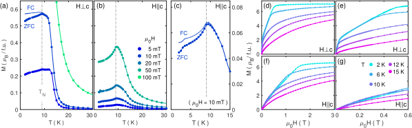
Figure 2: (color online). Direction-resolved SQUID magnetization measurements of EuCd₂As₂. Low-temperature thermal variation of the magnetization in magnetic fields between 5 and 100 mT applied along the (a) $a$ axis, and (b) $c$ axis. For 10 mT data, an enlarged comparison of field-cooled (FC) and zero-field-cooled (ZFC) data is shown in (c). All data were recorded upon warming. Field sweeps of the magnetization at temperatures between 2 and 15 K, in a field oriented (d) within the basal plane and (f) almost parallel to the $c$ axis. Panels (e) and (g) give a magnified view of the respective low-field data.

As determined in the present study, the magnetic propagation vector in the antiferromagnetic state of EuCd₂As₂ is $\textbf{q}_{\textrm{m}}=(0,0,0.5)$, and thus the magnetic unit cell contains only two, antiparallel, magnetic moments $\bf{m}$ at fractional coordinates $\textbf{r}_{1}=(0,0,0)$ and $-\textbf{m}$ at $\textbf{r}_{2}=(0,0,1)$. The magnetic structure factor vector in the reference frame of the crystal is therefore

$$\textbf{M}_{\textrm{cryst}}=\sum_{j}\textbf{m}_{j}\exp({\textrm{i}\textbf{q}_{\textrm{m}}\cdot\textbf{r}_{j}})=2\,\textbf{m}\,.$$ (2)

The determination of the magnetic structure thus reduces to the measurement of the orientation of $\bf{m}$ through its projections onto the cross product of linear polarization vectors [see Eq. (1)].

For a continuous rotation of the angle $\eta$ of the incident linear polarization $\hat{\bf{\epsilon_{i}}}$, a pair of diamond phase plates (300 $\mu$m thickness, $\approx 48\,$% transmission) is inserted in the incoming beam Francoual et al. (2013); Strempfer et al. (2013). The angle $\eta^{\prime}$ ($\hat{\bf{\epsilon_{f}}}$) of linearly polarized components of the scattered beam was selected by rotation of a Cu (110) analyzer crystal (at a scattering angle of $2\theta_{\mathrm{A}}\approx 90^{\circ}$) around $\hat{\bf{k}}_{f}$ sup . The polarization state of an x-ray beam is described by its Poincaré-Stokes vector ($P_{1}$,$P_{2}$,$P_{3}$), as defined in the Supplemental Material sup . In this REXS experiment, we measured the parameters $P_{1}^{\prime}$ and $P_{2}^{\prime}$ of the scattered beam as a function of the angle $\eta$ of the incident linear polarization sup .

We used the Quantum Espresso suite Giannozzi et. al. (2009) to perform electronic structure calculations of EuCd₂As₂. To treat the strong electronic correlations in the highly localized rare-earth 4$f$ states, a Hubbard term $U=3.1$ eV was included. This term adds an energy cost to the site-hopping of the 4$f$ electrons, which yields a magnetic moment that is consistent with the spin state $S=7/2$ of localized Eu²⁺. To account for the possible spin splitting of the bands due to the magnetic ions, the local spin density approximation was used as the exchange correlation. Given the presence of the heavy element Cd, relativistic pseudopotentials were also implemented in the plane wave electronic structure code to account for spin–orbit coupling. A Monkhorst–Pack k-point sampling mesh of $8\times 8\times 6$ was used Monkhorst and Pack (1976).

III III. Experimental Results

III.1 A. Magnetization

The temperature- and field-dependence of the magnetization is summarized in Fig. 2. The temperature sweeps reveal a magnetic ordering transition with unusual characteristics. A strong divergence of the magnetization is seen below about 20 K, which is arrested at around 13 K. The transition to antiferromagnetic order is signaled by a sharp change in slope at around 9 K.

The magnetic behavior is consistent with previous studies Artmann et al. (1996); Schellenberg et al. (2011), and had been interpreted as two distinct, consecutive, ferro- and antiferromagnetic phases by some authors Artmann et al. (1996). However, these earlier studies had not been direction-selective. In panels (a) and (b) of Fig. 2, we compare data obtained with the magnetic field parallel to the $a$ and $c$ axis, respectively. This reveals that the magnetic state is strongly anisotropic, with an in-plane susceptibility about 7 times larger than the out-of-plane susceptibility. The in-plane response is also qualitatively different, in that it appears to saturate and form a plateau, 2–3 K above the onset of antiferromagnetism.

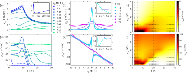
Figure 3: (color online). Alternating-current six-point electronic transport data of EuCd₂As₂, recorded with a 5 mA, 30 Hz excitation and magnetic fields applied along the $c$ axis. The characteristics of the in-plane longitudinal resistivity $\rho_{xx}$, and transversal (Hall) resistivity $\rho_{xy}$ are summarized in the top and bottom panels, respectively. (a),(d) Thermal variation at magnetic fields between 0 and 7 T. (b),(e) Field sweeps at temperatures between 2 and 70 K. The insets give a magnified view of subtle features in the low temperature data. (c),(f) Phase diagrams represented by color maps of interpolated data. Black markers indicate the actual location of data points.

The comparison of temperature sweeps recorded in field-cooled (FC) and zero-field-cooled (ZFC) conditions shows a splitting, see Fig. 2 (a) and (c), which is more significant for $\bf{H}\perp\bf{c}$ ($\approx 10\%$). For this geometry, the effect is consistent with the preferred alignment of antiferromagnetic domains, as observed in our REXS study and discussed in Section IV. In-plane rotations of AFM domains would not be expected to cause a FC–ZFC splitting for $\bf{H}\parallel\bf{c}$, and the weak splitting observed in Fig. 2(c) is most likely attributable to a small misalignment of the crystal giving contamination from the $\bf{H}\perp\bf{c}$ signal. For very low applied fields, $\mu_{0}H<50\,$mT, another anomaly appears in the out-of-plane susceptibility, which is seen as an additional decrease of the signal [below about $3\,$K at the lowest field, 5 mT, see Fig. 2 (c)]. This feature has not been observed previously and its origin is presently not known.

Field sweeps of the in-plane and out-of-plane magnetization are shown in Fig. 2 (d)–(g). As had been reported previously, the saturation magnetization approaches the value of $7\,\mu_{\text{B}}$ expected for an ideal Eu²⁺ ($4f^{7}$, $S=\nicefrac{{7}}{{2}}$, $L=0$) state Artmann et al. (1996); Schellenberg et al. (2011). At base temperature (2 K) and with a field applied along the $c$-axis, this saturation is achieved already in a relatively low field of $1.55\,$T. The $\bf{H}\parallel\bf{c}$ curve shows no evidence for any spin-flop transitions, but there is a subtle change in slope around 200 mT (at 2 K). By contrast, the application of a mere $50\,$mT within the basal plane sees a jump of the magnetization to around one third of its saturation value, followed by a steep linear increase and saturation near $0.5\,$T. An interpretation of these characteristics is provided below, in light of the REXS results.

III.2 B. Electronic transport

In the top and bottom panels of Fig. 3, we summarize the low temperature characteristics of the longitudinal resistivity $\rho_{xx}$ and transversal (Hall) resistivity $\rho_{xy}$, respectively. Above $\sim$80 K, the resistivity temperature sweep indicates a weak semimetallic behavior, see Fig. 3 (a) and inset. However, at lower temperatures, the resistivity increases by up to 100% and forms a sharp peak at $T_{\text{N}}=9.5\,$K. This is reminiscent of the corresponding magnetization characteristics shown in Fig. 3 (a), although the anomalous increase in resistivity sets in at even higher temperatures $\approx 50\,\text{K}\approx 5\,T_{\text{N}}$. When a magnetic field is applied (out-of-plane), this resistivity peak splits into two broad features: one with a leading edge that moves to higher temperatures in higher fields, and another, separated by a dip (minimum) of $\rho_{xx}$. By comparison with the magnetization data, it can be inferred that this minimum corresponds to the magnetic phase boundary, and, accordingly, disappears with the complete spin alignment at $1.55\,$T — see Fig. 2 (f).

The field sweeps of this resistivity signal, Fig. 3 (b), emphasize a strong negative magnetoresistance, corresponding to a $\approx 75\%$ reduction of the measured signal at 2 K. Within the magnetically ordered phase, the negative magnetoresistance is clearly associated with the spin-alignment, as it abruptly ends at the magnetization saturation field of $1.55\,$T. Another magnetoresistive feature is observed at temperatures above the ordering transition. It does not set in continuously, but is delineated by a clear kink in the field sweep — see data for 20 K in Fig. 3 (b).

The features discussed above can all be recognized in the phase diagram of interpolated resistivity data presented in Fig. 3 (c). Here, the magnetically ordered phase corresponds to a dark patch with a black-to-orange gradient. The regime of strong negative magnetoresistance appears as a yellow-to-white gradient and forms a diagonal phase line from the ordered phase towards high fields and high temperatures.

The characteristics of the Hall resistivity are summarized in the corresponding lower panels (d)–(f) of Fig. 3 and are governed by a similar phase diagram. In particular, the effective charge transport is hole-like and is superposed by two anomalous contributions: one which is confined to the magnetically ordered phase, and a distinct Hall contribution associated with the spin-polarized state for $T>T_{\textrm{N}}$, which is clearly delineated by a diagonal phase line.

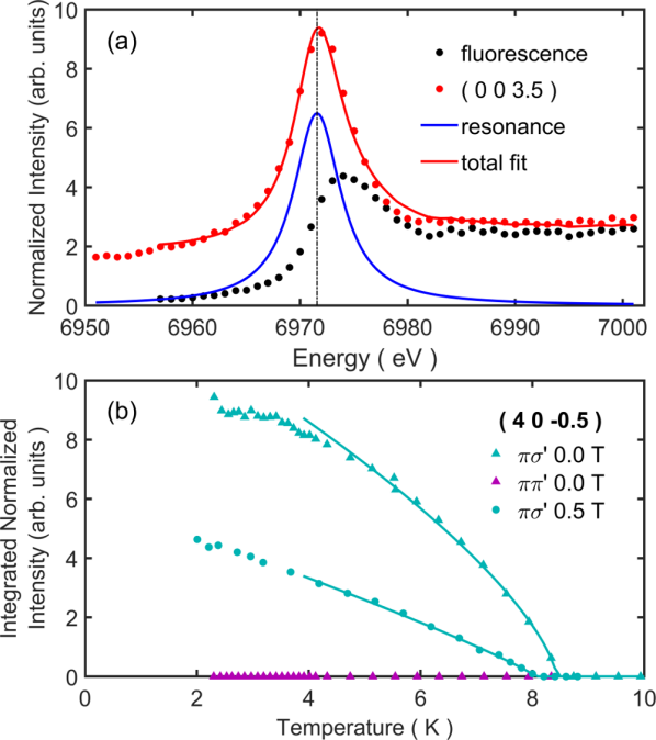
Figure 4: (color online). (a) Energy scans at the Eu $L_{3}$ resonance, recorded without polarization analysis of the scattered beam. The magnetic resonance at the $(0,0,3.5)$ reflection can be decomposed into a contribution due to x-ray fluorescence (black markers) and a Lorentzian peak centered in the pre-edge region, at 6972 eV. (b) Thermal variation of the $(4,0,-0.5)$ integrated peak intensity, recorded at zero field and with $0.5\,$T applied along the $c$ axis. The solid lines indicate fits of a power law $(T_{\text{N}}-T)^{2\beta}$ to the data ($T_{\mathrm{N}}=8.43(3)$, $\beta=0.34(1)$ for $\pi\sigma^{\prime}$ at 0 T). In the $\pi\pi^{\prime}$ channel no magnetic peak is observed.

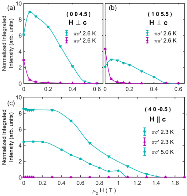
Figure 5: (color online). Field dependence of EuCd₂As₂ resonant magnetic x-ray scattering observed in the $\pi\sigma^{\prime}$ and $\pi\pi^{\prime}$ polarization channels. (a)–(b) For fields applied in the $a$-$b$ plane of the crystal, the scattered intensity abruptly switches from $\pi\pi^{\prime}$ to $\pi\sigma^{\prime}$ character at $\approx 50\,$mT and is then fully suppressed at $\approx 0.5\,$T. (c) When a magnetic field is applied parallel to the $c$ axis, $\approx 1.5\,$T is required to fully spin-polarize the sample. Solid lines are intended as visual guides.

III.3 C. REXS

Upon cooling below $T_{\text{N}}$, scans along high-symmetry directions in reciprocal space revealed that the magnetic propagation vector in EuCd₂As₂ is $\textbf{q}_{\textrm{m}}=(0,0,0.5)$. This is consistent with other magnetic materials of the same structural family for which neutron studies have been possible, such as EuMn₂P₂ [Payne et al., 2002] and EuAl₂Si₂ [Schobinger-Papamantellos and Hulliger, 1989]. We did therefore not perform a systematic search for additional propagation vectors. In Fig. 4 (a), constant wave vector energy scans at the $(0,0,3.5)$ reflection (measured without polarization analysis) are compared with the x-ray fluorescence measured at a scattering angle $2\theta=90^{\circ}$, where charge scattering vanishes. This signal, which is equivalent to an x-ray absorption (XAS) measurement, shows no indication of the Eu³⁺ valence (this would be associated with a peak about 8 eV above the Eu²⁺ $L_{3}$ absorption maximum Sun et al. (2010)). In addition to this fluorescence contribution, the intensity at the (0,0,3.5) position features a Lorentzian-like peak resonating in the pre-edge region at 6972 eV. This photon energy was selected for the remainder of the experiment.

After locating the magnetic Bragg peaks, we tracked the field- and temperature dependence of integrated magnetic intensities in the $\pi\sigma^{\prime}$ and $\pi\pi^{\prime}$ polarization channels. Given the form of the scattering amplitude, Eq. (1) (with reference to the $\hat{\bf{u}}_{i}$ reference frame sup ), these channels probe magnetic Fourier components parallel and perpendicular to the scattering plane, respectively. Fig. 4 (b) shows the thermal variation of these integrated intensities for the $(4,0,-0.5)$ peak, in zero field and for 0.5 T applied $5^{\circ}$ away from the $c$ axis.

The intensity in the $\pi\sigma^{\prime}$ channel follows a clear order parameter behavior, as described by a power law. The obtained Néel temperatures are $T_{\mathrm{N}}=8.43(3)$ K (0 T) and 8.08(2) K (0.5 T). By attenuating the beam, we confirmed that the reduction by $\approx 1\,$K from the expected value is due to beam heating. We note that beam heating did not affect the FLPA scans (discussed below), since the beam is attenuated by insertion of the phase plates. The critical exponent obtained from the power-law fit is $\beta=0.34(1)$ (0 T). This agrees with the values expected for the 3D Ising model ($\beta=0.3250$) or 3D $XY$-antiferromagnet ($\beta=0.3460$). This points to a three-dimensional character of the antiferromagnetic state in EuCd₂As₂ Le Guillou and Zinn-Justin (1977), although $\beta$ may also be slightly altered by beam heating.

In the $\pi\pi^{\prime}$ channel, no magnetic Bragg peak is observed at the $(4,0,-0.5)$ position. This indicates that there are no sizable $\bf{q}_{\text{m}}$ magnetic Fourier components perpendicular to the scattering plane, i.e. parallel to the $c$-axis.

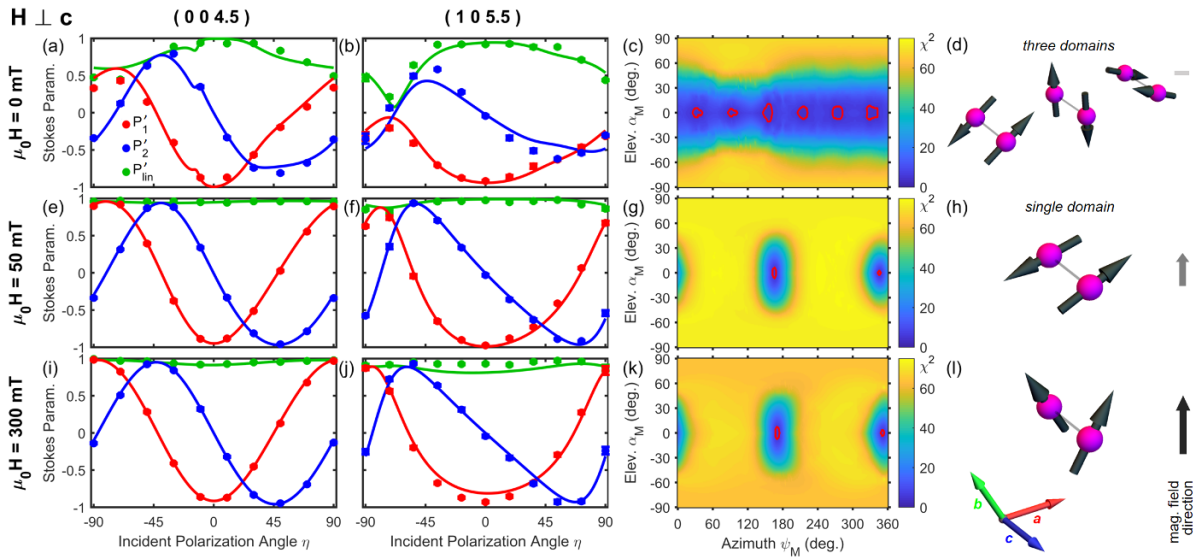
Figure 6: (color online). Full polarization analysis of the $(0,0,4.5)$ and $(1,0,5.5)$ magnetic reflections of EuCd₂As₂, in zero field (top row) and with magnetic fields of 50 and 300 mT applied within the $ab$ plane (middle and bottom rows). The left columns show the best fits (lines) to the Stokes parameters $P_{1}^{\prime}$, $P_{2}^{\prime}$ and $P_{\text{lin}}^{\prime}=\sqrt{P_{1}^{\prime 2}+P_{2}^{\prime 2}}$ extracted from the polarization scans. Panels (c), (g) and (k) show the corresponding $\chi^{2}$ maps of least squares fits performed with the angles ($\psi_{M}$, $\alpha_{M}$) held fixed (discussion cf. main text). Panels (d), (h) and (l) illustrate the respective moment directions in adjacent layers. Where applicable, the three magnetic domains are indicated.

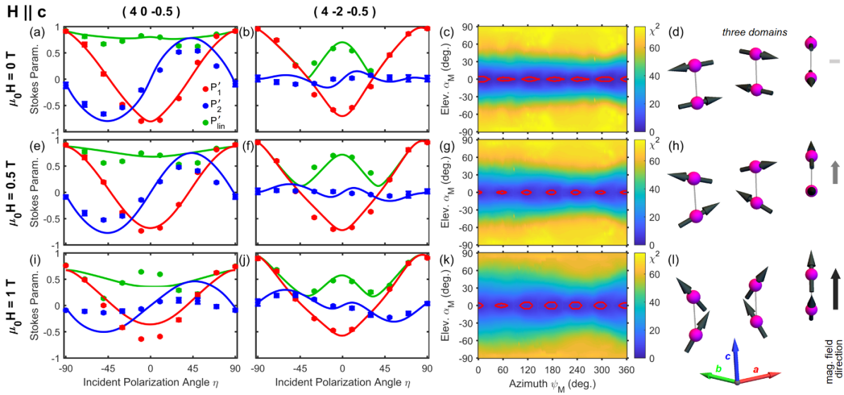
Figure 7: (color online). Full polarization analysis of the $(4,0,-0.5)$ and $(4,-2,-0.5)$ magnetic reflections of EuCd₂As₂, in zero field and with magnetic fields of 0.5 and 1 T applied almost parallel to the $c$ axis. The figure is organized in analogy to Fig. 6. In all cases, fits using three domains were superior to models using a single domain or an isotropic distribution of azimuthal moment orientations. In applied fields, the magnetic intensity at the $\bf{q}_{\mathrm{m}}=(0,0,0.5)$ magnetic Bragg peaks subsides and the relative intensity of diffuse charge scattering becomes substantial. Due to these increasing background contributions in the $\pi\pi^{\prime}$ and $\sigma\sigma^{\prime}$ channels, the Stokes parameter fit quality deteriorates at higher fields.

The field dependences of three magnetic peaks at base temperature ($2.3\,$K) are shown in Fig. 5. Again, the $(0,0,4.5)$ and $(1,0,5.5)$ peaks correspond to an in-plane magnetic field, whereas for $(4,0,-0.5)$, the $c$ axis is directed $5^{\circ}$ away from the magnetic field axis. Both $\bf{H}\perp\bf{c}$ -type peaks, Figs. 5 (a) and (b), show a transition at a low field of $\approx 50\,$mT, where magnetically scattered intensity changes abruptly from the $\pi\pi^{\prime}$ to the $\pi\sigma^{\prime}$ channel. As noted above, this implies a switching of antiferromagnetic Fourier components, which are initially perpendicular to the scattering plane, into the scattering plane. By $0.5\,$T applied in-plane, the $\pi\sigma^{\prime}$ intensity has also completely disappeared. At this point the sample is fully spin-polarized, i.e. all magnetic intensity would be located at the $\Gamma$ point of the Brillouin zone.

A different behavior is observed for the almost  $\bf{H}\parallel\bf{c}$ -like situation shown in Fig. 5 (c). Here, no magnetic intensity is observed in the $\pi\pi^{\prime}$ channel, i.e. the magnetic structure has no $\bf{q}_{\mathrm{m}}=(0,0,0.5)$ Fourier component perpendicular to the scattering plane. The intensity in the $\pi\sigma^{\prime}$ channel varies little up to $\approx 0.4\,$T and then decreases monotonically. By contrast to panels (a) and (b), a much larger field of $\approx 1.5\,$T is required to fully spin-polarize the material (at 2.3 K), which is consistent with the magnetization field sweeps shown above in Figs. 2 (d)–(g).

The two left columns of Figs. 6 ($\bf{H}\perp\bf{c}$) and 7 ($\bf{H}\parallel\bf{c}$) show the Stokes parameters $P_{1}^{\prime}$ and $P_{2}^{\prime}$ and degree of linear polarization $P_{\text{lin}}^{\prime}=\sqrt{P_{1}^{\prime 2}+P_{2}^{\prime 2}}$ describing the polarization state of x-rays scattered at two magnetic reflections, at zero field (top row), and with increasing strength of an applied magnetic field (second and third row). These measurements were all performed at base temperature ($\approx\,2.3\,$K). The determination of the Stokes vector ($P_{1}^{\prime},P_{2}^{\prime}$) from full polarization analysis is discussed in the Supplemental Material sup . Due to our observation of an anomaly at $T\approx 3\,$K in the magnetic susceptibility data (see Fig. 2) we investigated specifically the possibility of a distinct low-temperature magnetic phase at zero field. However, we did not observe any variation in the polarization characteristics of the magnetic scattering (at zero field). Nevertheless, the possibility of some weak remaining beam heating to $T>3\,$K (with phase retarding plates in the beam) cannot be excluded.

As a first observation, several datasets [Figs. 6 (a),(b) and 7 (a), (b), (e), (f), (i), (j)] show a significant reduction in the degree of linear polarization of the scattered beam ($P_{\text{lin}}^{\prime}$, see green markers). We identified two causes that contribute to this effect.

Firstly, the effective observed Stokes parameters may vary if the signal is contaminated by diffuse charge scattering contributions. This adds to the dipole scattering amplitude, Eq. (1), a term of the form Hill and McMorrow (1996)

$$\hat{\bf{\epsilon}}_{f}\cdot\hat{\bf{\epsilon}}_{i}=\begin{pmatrix}1&0\\ 0&\hat{\bf{k}}_{f}\cdot\hat{\bf{k}}_{i}\end{pmatrix}=\begin{pmatrix}1&0\\ 0&\cos 2\theta\end{pmatrix}~{}~{}.$$ (3)

The effect therefore becomes important for peaks at large scattering angles when the sample is almost spin-polarized and when antiferromagnetic scattering is weak. In Section 7 of the Supplemental Material sup , we illustrate this effect by comparison of $2\theta$-scans at the $(4,0,-0.5)$ position (at $2\theta=136.6^{\circ}$), in the $\pi\pi^{\prime}$ and $\pi\sigma^{\prime}$ polarization channels. At 1 T, corresponding to the FLPA shown in Fig. 7 (i), the background intensity in the $\pi\pi^{\prime}$ channel is about $7\,\%$ of the magnetic signal seen in $\pi\sigma^{\prime}$. In fact, when considering panels (a), (b), (e), (f), (i), (j) of Fig. 7, it can be recognized that the Stokes parameter $P_{1}^{\prime}$ continuously becomes more “$\cos 2\eta$ -like” and $P_{2}^{\prime}$ becomes more “$-\sin 2\eta$ -like” as the magnetic field is applied. In effect, these anti-phase contributions decrease the amplitudes of both $P_{1}^{\prime}$ and $P_{2}^{\prime}$, and so $P_{\text{lin}}^{\prime}=\sqrt{P_{1}^{\prime 2}+P_{2}^{\prime 2}}$ is no longer unity.

Nevertheless, these background contributions do not account for the decrease in $P_{\text{lin}}^{\prime}$ in the case of Fig. 7 (a) and (b), where the magnetic intensity is dominating the observed signal. We find that this can be modeled by taking into account the formation of magnetic domains in EuCd₂As₂. In general, it must be expected that a zero-field–cooled sample will contain all symmetry-equivalent magnetic domains, the scattered intensities of which add. Antiphase signals from different domains can thus introduce circular components to the scattered beam. For trigonal EuCd₂As₂, three equivalent magnetic domains would be expected if the magnetic moments are not aligned strictly along the $c$ axis.

IV IV. Analysis and interpretation

Taking into account the above considerations, our experimental results can be explained as follows [see panels (d,h,l) of Figs. 6 and Fig. 7]. The magnetic structure of EuCd₂As₂ consists of ferromagnetic layers which are stacked antiferromagnetically, in other words, an A-type antiferromagnet. Even though the Eu²⁺ state has no orbital angular momentum, the magnetic moments experience a weak magnetocrystalline and/or dipolar anisotropy which favors spin alignment along specific directions in the $a$-$b$ plane, as already illustrated in Fig. 1. The trigonal crystal symmetry generates three equivalent antiferromagnetic domains, related by $120^{\circ}$ rotation (i.e. six possible orientations of the spins), and if the domains are smaller than the volume of the sample probed by the x-rays, then the measured magnetic scattering intensity will be a sum of the intensities for each domain, weighted by the population of each domain.

For each pair of FLPA scans in Figs. 6 and 7, we show a $\chi^{2}$ map of least squares fits with fixed magnetic moment directions [see panels (c,g,k)]. We represent the orientation of the $\bf{q}_{\textrm{m}}=(0,0,0.5)$ Fourier component of the magnetic structure by the azimuth and elevation ($\psi_{\text{m}}$, $\alpha_{\text{m}}$) in an orthonormal reference frame determined by the crystallographic $a$ and $c$ axes. These angles are defined and illustrated in Section 5 of the Supplemental Material sup , where we also describe the transformation of $\bf{m}_{\mathrm{cryst}}$ to the $\hat{\bf{u}}_{i}$ reference-frame. Red contours imposed onto these $\chi^{2}$ maps delineate the parameter range corresponding to one standard deviation from the best fit parameters.  
 
For zero applied field, both measurements [panels (a)–(b) of Figs. 6 and 7] yielded superior fits when the three-fold domain population was allowed to vary. The quality of the fits allows us to exclude definitively the possibility that the magnetic moments have a significant out-of-plane antiferromagnetic component. On the other hand, the fits do not reveal a unique azimuthal orientation $\psi_{\text{m}}$. Instead, the two crystals investigated favor different orientations, with best fits at $\psi_{\text{m}}\approx 37^{\circ}$ and $\psi_{\text{m}}\approx 0^{\circ}$ for the $\bf{H}\perp\bf{c}$ and $\bf{H}\parallel\bf{c}$ samples, respectively [see red contour lines in panels (c) of Figs. 6 and 7]. This may indicate a lack of significant in-plane anisotropy, or a dependence on sample history. Nevertheless, in all cases, it was not possible to obtain an improved fit to the data with a continuous (i.e. not three-fold discrete) distribution of azimuthal moment directions.

When a $50\,$mT in-plane magnetic field is applied, Fig. 6 (e)–(h), $P_{\text{lin}}^{\prime}$ is restored to unity throughout and the Stokes parameters can be perfectly reproduced by a one-domain model with the magnetic moments aligned almost perpendicular to the applied field (which happens to be close to the $a$ axis in this experiment). This behavior corresponds to a spin-flop–like redistribution of domain populations, before all moments can be continuously canted into the field direction. The small magnitude of the magnetic field which effects this domain-flop reflects the weakness of the dipolar coupling between antiferromagnetic domains. This model also naturally explains the $\bf{H}\perp\bf{c}$ field sweeps shown in Fig. 5 (a,b) and discussed above. Increasing the in-plane field to 300 mT, see Fig. 6 (i)–(l), suppresses the antiferromagnetic Bragg peaks as the moments cant towards the field direction and intensity is redistributed to the Brillouin zone center, but the Stokes parameter scans are hardly changed.

As expected in this model, the selection of a single domain does not occur if the field does not break the three-fold symmetry. Accordingly, all results shown in Fig. 7 were better modeled by imposing the three-fold domain structure. However, since this crystal was actually mounted with the $c$ axis tilted $5^{\circ}$ from the magnet axis, one domain (the only direction in which the magnetic moments lie both in the $a$–$b$ plane and in the scattering plane) is clearly favored by the fits. As the out-of-plane field is successively increased to 0.5 and 1 T, the favored moment direction (close to the $a$ axis) does not change. Instead, the continuous change in Stokes parameter characteristics is attributed to the increasing relevance of the diffuse charge scattering background, as the magnetic intensity subsides.

V V. Discussion

In EuCd₂As₂, the in-plane ferromagnetic correlations are expected to be much stronger than the inter-plane antiferromagnetic exchange interactions (six in-plane ferromagnetic nearest neighbors vs. two more distant antiferromagnetic neighbors along the $c$ axis). This explains the continuous onset of short-range in-plane ferromagnetic correlations that starts at $T\gg T_{\text{N}}$, Fig. 2 (a)–(b), and leads to an incipient ferromagnetic-like transition, before the pre-formed ferromagnetic planes lock into an antiferromagnetic stacking at $T_{\textrm{N}}$.

We find that the magnetic susceptibility of EuCd₂As₂ at $T\lesssim T_{\textrm{N}}$ is about 7 times larger for magnetic fields applied in the $a$–$b$ plane than for fields along the $c$ axis. For a conventional antiferromagnet, it is expected that the magnetic state is softer for magnetic fields applied perpendicular to the moment direction. On this basis one might therefore infer an out-of-plane moment direction (as done by Wang et al. Wang et al. (2016a)). However, in the present case, the magnetic moments are actually lying in the $a$–$b$ plane, and, owing to the three-fold domain structure, EuCd₂As₂ can avoid a conventional spin-flop transition irrespective of the field direction. Instead, the anisotropy of the susceptibility is mainly a measure of the easy-plane anisotropy and the fact that the spins point in different in-plane directions within each domain. The easy-plane anisotropy is also reflected in the fact that the saturation field is smaller for $\bf{H}\perp\bf{c}$ than for $\bf{H}\parallel\bf{c}$ ($0.5\,$T vs. $1.5\,$T).

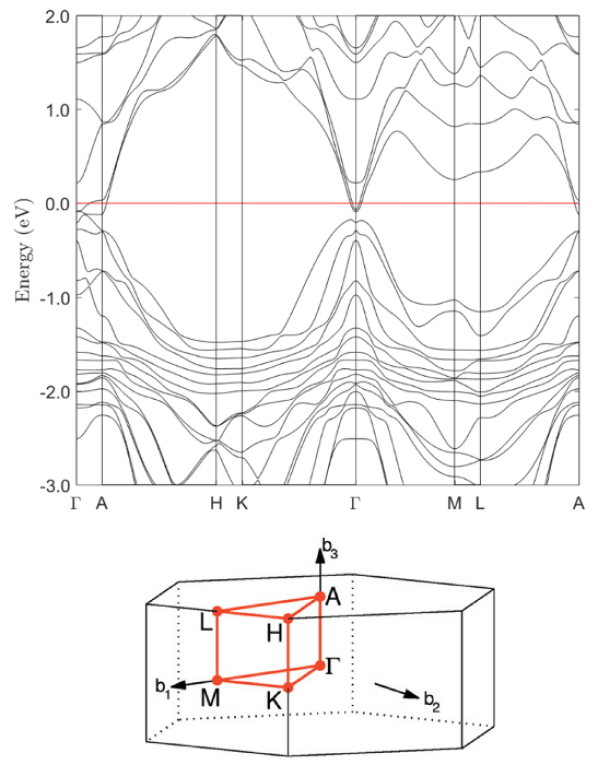
Figure 8: (color online). Calculated electronic structure of EuCd₂As₂ along high symmetry lines of reciprocal space. The conventional labeling of high symmetry points in the Brillouin zone of the hexagonal lattice is indicated below Setyawan and Curtarolo (2010).

It is interesting to consider the resistivity and Hall resistivity characteristics in the light of this model. For small applied fields, anomalous Hall effect (AHE) contributions in the multi-domain state will cancel. On the other hand, at sufficiently large fields that the in-plane ferromagnetic order becomes ferromagnetically aligned in the $c$ direction, a sizable anomalous Hall effect would be expected, both above and below the (3D) magnetic ordering temperature Nagaosa et al. (2010). With increasing thermal fluctuations, the alignment of pre-formed 2D ferromagnetic planes will require stronger applied fields, which explains the diagonal phase line observed in Fig. 3 (f). If the full spin alignment reduces the scattering of charge carriers from magnetic fluctuations, the above $\rho_{xy}$ argument simultaneously explains the corresponding “inverse” $\rho_{xx}$ phase diagram of Fig. 3 (c).

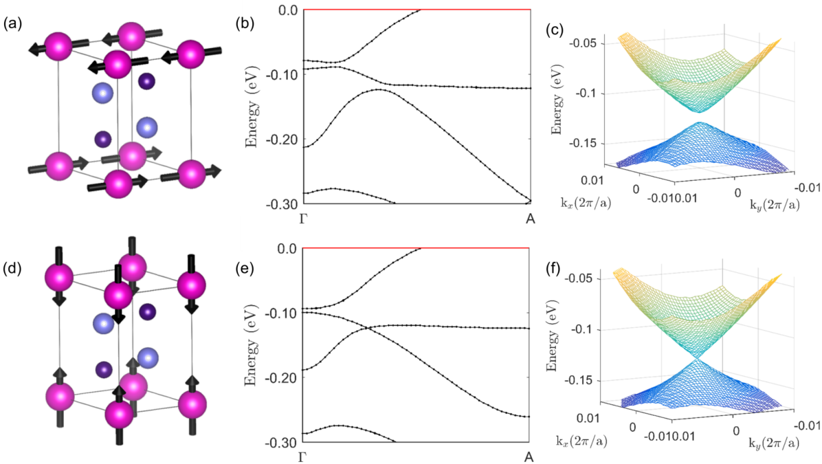
Figure 9: (color online). Calculated electron bands near $E_{\textrm{F}}$ for A-type antiferromagnetic order in EuCd₂As₂. (a)–(c) Spins lying in the $a$–$b$ plane, as found experimentally, and (d)–(f) spins along the $c$ axis. The calculated dispersion $E(k_{z})$ along the $\Gamma$–A high symmetry line corresponding to these magnetic states is presented in (b) and (e), and detailed views of $E(k_{x},k_{y})$ in the vicinity of the Dirac band crossing are shown in (c) and (f). This crossing is gapped for in-plane spins, as shown in (c), but is protected by $C_{3}$ symmetry for spins parallel to the $c$ axis resulting in Dirac points at $\textbf{k}=\pm(0,0,0.16)$, as shown in (f).

On the other hand, this explanation does not encompass the transport characteristics within the antiferromagnetically ordered phase. Contrary to observation, no large AHE contribution would be expected in the antiferromagnetic state (but only when a significant net ferromagnetic component is induced by an applied magnetic field). The insets of Figs. 3 (b) and (e) show both large longitudinal and transversal resistivity contributions that are effectively proportional to the antiferromagnetic component measured by REXS, see Fig. 5 (c). This implies a more subtle coupling between the magnetic state and the electronic transport.

VI VI. Ab initio electronic structure

Density functional calculations of the $\textbf{q}_{\textrm{m}}=(0,0,0.5)$ A-type antiferromagnetic state of EuCd₂As₂ were performed in the magnetic unit cell (i.e. in a cell doubled along the $c$ axis relative to the crystallographic cell). The orientation of the in-plane Eu magnetic moments was defined as shown in Fig. 1 (a). In Fig. 8 we show the calculated electronic band dispersion along high-symmetry directions in the Brillouin zone. At binding energies between 1.5–2.0 eV, the system is dominated by weakly dispersing Eu 4$f$ bands. This suggests that these electrons are strongly localized, which is consistent with the prevailing picture for divalent Eu. The calculated ordered magnetic moment per Eu of the $4f$ states is $\mu=6.93$ $\mu_{\textrm{B}}$, corresponding to $\mu_{\text{eff}}=$ 7.86 $\mu_{B}$, in good agreement with the estimates from magnetometry.

This binding energy of Eu 4$f$ bands is highly sensitive to the magnitude of the Hubbard-like $U$ parameter Schlipf et al. (2013); An et al. (2011). As typically seen in DFT calculations Kotliar and Vollhardt (2004), neglect of the electronic correlations $U$ would lift the 4$f$ bands to the Fermi level. Under these circumstances, one would predict EuCd₂As₂ to be a good metal Larson and Lambrecht (2006); Kuneš et al. (2005); Ingle and Elfimov (2008). Indeed, earlier computational work by Zhang et al. suggested that this is the case in isostructural EuCd₂Sb₂, see Refs. Zhang et al., 2010a and Zhang et al., 2010b. This scenario is appealing, because it allows to attribute magnetoresistive effects to the shifting of the Eu 4$f$ bands across the Fermi level, i.e. the magnetic bands would themselves contribute to the charge transport.

However, preliminary ARPES measurements on EuCd₂As₂ have ruled out this possibility Schröter and et al. (2016). Instead, the 4$f$ bands are observed $\approx 1.5$ eV below the Fermi level, and we have used a Hubbard parameter $U=3.1$ eV to reflect this in our calculation. This is also consistent with the semimetallic in-plane and inter-plane behavior of EuCd₂As₂ that was previously reported by Wang et al. Wang et al. (2016b). The orbital character analysis of our density functional study confirms that the conduction and valence bands are dominated by the Cd 5$s$ and As 4$p$ states, respectively (see Section 8 of the Supplemental Material sup ). This implies that charge transport is confined to the Cd–As double-corrugated trigonal layers, which are spaced by insulating magnetic Eu layers.

Our calculations also show that the conduction and valence bands exhibit a two-fold degeneracy without spin splitting, despite the presence of the magnetic Eu species. Moreover, due to the strong spin–orbit coupling in the heavy-element Cd–As sublattice, these bands are inverted at the $\Gamma$ point in the Brillouin zone, i.e. at this point the bands with Cd 5$s$ orbital character reside below that with As 4$p$ character. All these qualities bear striking resemblance to those of the three-dimensional topological Dirac semimetal Cd₃As₂: (1) the electronic properties are determined by the Cd 5$s$ and As 4$p$ states, (2) there is an inversion of the aforementioned bands at the $\Gamma$ point, and (3) the bands are all doubly-degenerate Liu et al. (2014b); Neupane et al. (2014); Wang et al. (2013).

In light of these analogies, we searched the Brillouin zone for similar topologically non-trivial features to those found in Cd₃As₂, and indeed identified a linear band crossing along the $\Gamma$–A high symmetry line at $k_{z}=\pm 0.16\,$Å^-1, with a gap of $\approx 10$ meV, see Fig. 9 (a)–(c). This energy gap is not induced by broken time-reversal symmetry because spatial inversion symmetry is simultaneously broken in EuCd₂As₂, and so the product of the two symmetries is conserved. Instead, this gap arises because the $C_{3}$ symmetry along the $\Gamma$–A line which protects the Dirac crossing point is broken by the magnetic order in which, as found here, the spins lie parallel to the $a$–$b$ plane. This gap will close if the $C_{3}$ symmetry is preserved, e.g. for a magnetic structure in which the spins lie along the c-axis as shown in Fig. 9 (d)–(f). As the spins lie in the $a$–$b$ plane this result suggests that the magnetic ground state of EuCd₂As₂ does not harbor massless Dirac fermions. The extent to which massive Dirac fermions influence the transport in EuCd₂As₂ remains to be established and, in addition, the possibility of surface states due to the non-trivial topology in the electronic structure cannot be excluded Hua et al. (2018).

VII VII. Conclusions

In conclusion, by comprehensive REXS experiments in applied magnetic fields, we have formed a consistent picture of the magnetic ground state of EuCd₂As₂. This demonstrates a successful application of REXS, in a material where neutron diffraction would be very difficult without isotopic enrichment with both Eu-153 and Cd-114. Using our understanding of the magnetic order we demonstrated that several distinct features in the resistivity can be understood in terms of field-induced domain alignment and/or spin reorientation.

Recently, Wang et al. reported an electrical and optical conductivity study of EuCd₂As₂ in which, based on resistivity measurements, an out-of-plane magnetic moment direction was postulated Wang et al. (2016a). The present findings show conclusively that the spins in fact lie in the $a$–$b$ plane.

It will be of great interest to perform photoemission and quantum oscillation measurements on EuCd₂As₂ to corroborate our computational study of the band topology and to establish the extent to which Dirac-like fermions influence the charge transport. Our results suggest that the CaAl₂Si₂ structure could host Dirac fermions that couple to a magnetically-ordered state at zero field. A possible route to achieve this is to search for related rare-earth based magnetic materials in which the magnetic order preserves the $C_{3}$ symmetry along the $\Gamma$–A line.

Note added: During the preparation of this manuscript a preprint appeared Hua et al. (2018) in which electronic structure calculations were reported for EuCd₂As₂. The authors consider various possible magnetic structures, though not the one found in our experiments. The authors do investigate the A-type antiferromagnetic structure with moments aligned parallel to the $c$ axis, Fig. 9 (d), and for this case the calculated band dispersion in Ref. Hua et al., 2018 is consistent with our results shown in Figs. 9 (e)–(f).

VIII Acknowledgments

1. Laboratory single crystal x-ray diffraction

As described in the manuscript, the flux-grown single crystals were characterized by laboratory single-crystal x-ray diffraction to confirm the structure and stoichiometry. The measurement was performed on a Agilent Supernova kappa-diffractometer, using a Mo $K_{\alpha}$ micro-focused source and an Atlas S2 CCD area detector Agilent Technologies XRD Products .

The trigonal crystal structure (space group $P\bar{3}m1$) of EuCd₂As₂ had been originally determined by Artman et al. Artmann et al. (1996), and is shown in Fig. S1 (c,d). The present single crystal diffraction dataset comprised 1077 Bragg reflections, which were indexed in a trigonal cell [$a,a,c,90^{\circ},90^{\circ},120^{\circ}$] with $a\approx 4.44\,$Å and $c\approx 7.33\,$Å. Intensity integrated over a margin perpendicular to high symmetry planes of reciprocal space is shown in Fig. S1 (a). In all directions, the average mosaicity was smaller than the instrumental resolution ($\approx 0.6$–$0.9^{\circ}$), which indicates the high crystalline quality of these samples. Rocking scans on the Huber diffractometer at beamline P09 confirmed a mosaicity of 0.15^∘ or better.

We also performed a refinement of the integrated Bragg intensities (FullProf algorithm Rodriguez-Carvajal (1993)). The best fit to the data is shown in Fig. S1 (b). Due to the heavy elements, absorption effects are strong and the comparison factor of equivalent reflections is high, $R_{\text{int}}=14\%$. Nevertheless, a satisfactory refinement ($R_{\text{F}}=3.74$) was achieved. The obtained atomic parameters, listed in Table I., are consistent with literature Artmann et al. (1996); Schellenberg et al. (2011). The refinement of atomic occupation factors confirmed the ideal stoichiometry of the sample.

Table 1: Results of the refinement of integrated single crystal x-ray diffraction intensities of EuCd₂As₂ (as illustrated in Fig. S1): Wyckoff sites of space group $P\bar{3}m1$, atomic positions, thermal parameters and site occupations. The observed peaks were indexed in a trigonal cell with lattice parameters $a\approx 4.44\,$Å and $c\approx 7.33\,$Å.

	Wyck.	$x$	$y$	$z$	$B$	occ. (%)
Eu	1a	0	0	0	1.08(6)	100
Cd	2d	$\nicefrac{{1}}{{3}}$	$\nicefrac{{2}}{{3}}$	0.6333(3)	1.27(7)	100
As	2d	$\nicefrac{{1}}{{3}}$	$\nicefrac{{2}}{{3}}$	0.2463(5)	1.09(7)	100

Fig. S1 (color online). Room temperature Mo $K_{\alpha}$ four circle x-ray diffraction of a $\approx\,200\,\mu\text{m}$ EuCd₂As₂ crystallite. (a,b) Perspective and top views of the trigonal structure of EuCd₂As₂. (c) Integration of the dataset over a small margin perpendicular to the ($HK0$) and, (d), ($H0L$) reciprocal lattice planes. (e) Integrated intensities sorted by momentum transfer $Q$, along with the refined values (FullProf Rodriguez-Carvajal (1993)) and the corresponding differences.

2. Six-point transport measurements

The resistivity and Hall effect measurements reported in the main text were performed using the alternating current transport (ACT) option of a physical properties measurement system (Quantum Design [Quantum Design, Inc., 10307 Pacific Center Court, San Diego, CA 92121, USA, ]). For all measurements, an excitation current of $5\,$mA, $30\,$Hz was applied in the $a$–$b$ plane and a magnetic field up to $10\,$T was applied along the crystallographic $c$ axis. The plate-like sample (thickness $\approx 200\,\mu m$) was contacted in a six-point geometry, such that longitudinal and transversal (Hall) voltage can be measured simultaneusly. This is illustrated in Fig. S2 along with the corresponding wiring of the sample holder.

Fig. S2 (color online). Sample geometry for alternating current transport measurements using (Quantum Design PPMS) Quantum Design, Inc., 10307 Pacific Center Court, San Diego, CA 92121, USA . (a) Wiring scheme of the PPMS sample holder using both lock-in amplifiers of the system to measure both longitudinal and transversal voltages. (b) EuCd₂As₂ single crystal contacted for a six-point measurement.

3. REXS setup at P09 (PETRA-III)

The second experimental hutch (EH2) of the hard x-ray diffraction experimental station P09 at PETRA-III (DESY) has three unique advantages for the present study: (1) Up to high energies (3.2–14 keV), the angle of the incident linear x-ray polarization can be rotated using a pair of diamond phase plates Francoual et al. (2013). (2) The non-magnetic heavy-load diffractometer holds a vertical 14 T cryomagnet. (3) In the sample space of the variable temperature insert, there is a continuous flow of exchange gas from the liquid helium reservoir. By comparison to closed cycle refrigerators, this reduces the effects of beam heating and allows cooling of the sample down to $T_{\text{base}}\approx 2.3\,$K.

Fig. S3 (color online). (a) Schematic of the horizontal scattering setup in the second experimental hutch of instrument P09, PETRA-III. The scattering triangle ($\bf{k}_{i}$, $\bf{k}_{f}$, $\bf{Q}$) for an arbitrary scattering angle $2\theta$ is shown, along with the definitions of the laboratory reference frame $(\bf{x},\bf{y},\bf{z})$ and the conventional scattering reference frame $(\hat{\bf{u}}_{1},\hat{\bf{u}}_{2},\hat{\bf{u}}_{3})$. (b) Perspective view of (a), which illustrates the orientation of the incident ($\hat{\epsilon}_{\sigma}$, $\hat{\epsilon}_{\pi}$) and scattered ($\hat{\epsilon}^{\prime}_{\sigma}$, $\hat{\epsilon}^{\prime}_{\pi}$) polarization vectors as well as the corresponding polarization angles $\eta$ and $\eta^{\prime}$. (c) Definition of the amplitudes of the linearly polarized light, parallel ($V_{1}$) and perpendicular ($V_{2}$) to the scattering plane (view towards the beam). (d,e) Full polarization analysis of the direct beam at a photon energy of 6.972 keV. The Stokes parameters shown in panel (e) confirm that the beam is fully linearly polarized for any setting of the phase retarder. Each set of ($P_{1}$, $P_{2}$) is obtained by fitting Eq. S6 to the integrated intensities (black markers) shown in panels (d). The best fit is indicated by a blue line.

The experimental setup of P09-EH2 is illustrated in Fig. S3. The experiment was performed in the horizontal scattering geometry. The hard x-ray beam penetrates the cryostat through thin beryllium windows, which imposes constraints on the detector angles $2\theta$ (azimuth) and $\gamma$ (elevation). To avoid a tilting of the heavy cryostat ($\chi$ axis), the instrument was effectively used as a two-circle diffractometer (with scattering angle $2\theta$ and a parallel sample rotation axis $\omega$). Small misalignments of the sample can be compensated by an elevation of the detector out of the horizontal plane ($-5^{\circ}<\gamma<5^{\circ}$). In principle, this tilts the scattering plane away from that shown in Fig. S3 (a,b), which complicates the polarization analysis. However, as only peaks with $\gamma<1.5^{\circ}$ were investigated, we neglect this effect in the data analysis.

In order to investigate the magnetic state with a magnetic field applied within the basal plane ($\bf{H}\parallel\bf{c}$), a crystal was polished with a surface parallel to the [001] plane and mounted with this (001) direction in the (horizontal) scattering plane. In this setting, the $(0,0,4.5)$ and $(1,0,5.5)$ magnetic reflections were accessible. Fig. S4 illustrates the scattering geometry for the case of $\bf{H}\parallel\bf{c}$. Here, it was desirable to access a $(h,0,-0.5)$-type magnetic Bragg peak with largest possible index $h$. To this end, a crystal was polished with a surface parallel to the $[100]$ crystal planes. A brass (non-magnetic) sample holder was then micro-machined with a $5^{\circ}$ tilt, such that the $(4,0,-0.5)$ direction is in the scattering plane and the field is applied only $5^{\circ}$ from the $c$ axis, see Fig. S4 (a–c). As shown in Fig. S4 (d), this left a narrow margin in reciprocal space in which $(h,k,-0.5)$-type peaks were accessible, delineated by the constraints in $\gamma$ and $2\theta$.

Fig. S4 (color online). (a) Micrograph of the crystal that was aligned and polished for $\bf{H}\parallel\bf{c}$-measurements. A surface parallel to the $[1,0,0]$ crystallographic planes has been prepared. (b) Technical drawing of a micro-machined sample holder for horizontal scattering with a 5^∘ offset from the sample surface. (c) Unit cell of EuCd₂As₂ viewed along the (100) direction. The $[4,0,-0.5]$ crystallographic plane is indicated by a black line. (d) View of the $(h,k,-0.5)$ plane of reciprocal space investigated in this sample. The dashed lines mark the constraints imposed by the maximum scattering angle ($2\theta$) and the vertical aperture of the Be windows ($\gamma$). Accessible $\bf{q}_{m}=(0,0,0.5)$ magnetic peaks are indicated by red markers.

4. FLPA formalism

A convenient formalism for the description of polarized x-ray scattering phenomena has been described by Detlefs et al. Detlefs et al. (2012). Useful discussions of full linear polarization analysis (FLPA) are also found in several reports of successful studies Mazzoli et al. (2007); Johnson et al. (2008); Hatton et al. (2009); Shukla et al. (2012); Francoual et al. (2015). Here we provide a brief summary of these concepts since they are relevant to the data presented in the main text.

The electric field $\bf{E}$ of an x-ray beam of energy $\hbar\omega$ and wave vector $\bf{k}$ can be decomposed into two orthogonal amplitudes $V_{1}$ and $V_{2}$.

$$\bf{E}(t,\bf{r})=\mathfrak{R}\left[(V_{1}\,\hat{\bf{\epsilon}}_{\sigma}+V_{2}\,\hat{\bf{\epsilon}}_{\pi})\cdot\,e^{-i(\omega t-\bf{k}\cdot\bf{r})}\right]~{}~{},$$ (S1)

where $\mathfrak{R}$ signifies the real part of this field. This is not relevant in the linearly polarized case, where the Jones polarization vector,

$$\hat{\bf{\epsilon}}=\begin{pmatrix}V_{1}\\ V_{2}\end{pmatrix}=\begin{pmatrix}\cos\eta\\ \sin\eta\end{pmatrix}$$ (S2)

has no imaginary components. As shown in Fig. S3 (a,b), the unit vectors $\hat{\bf{\epsilon}}_{\sigma}$, $\hat{\bf{\epsilon}}_{\pi}$ and $\hat{\bf{k}}_{i}$ form a right-handed coordinate system. For linearly polarized light, the Jones vector can thus be reduced to the polarization angle $\eta$, as indicated in Fig. S3 (c).

The polarization state of the beam is described by the Poincaré-Stokes vector $(P_{1},P_{2},P_{3})$, which is defined as

$$\begin{split}P_{1}&=\frac{|V_{1}|^{2}-|V_{2}|^{2}}{|V_{1}|^{2}+|V_{2}|^{2}}\\ P_{2}&=\frac{|V_{1}+V_{2}|^{2}-|V_{1}-V_{2}|^{2}}{2\,(|V_{1}|^{2}+|V_{2}|^{2})}\\ P_{3}&=\frac{(|V_{1}-i\,V_{2}|^{2}-|V_{1}+i\,V_{2}|^{2})}{2\,(|V_{1}|^{2}+|V_{2}|^{2})}\end{split}$$ (S3)

For fully linearly polarized light, $P_{3}$ vanishes and the degree of linear polarization is unity,

$$P_{\mathrm{lin}}=\sqrt{P_{1}^{2}+P_{2}^{2}}\rightarrow 1$$ (S4)

By combining Eqs. S2 and S3, it also follows that in this case

$$P_{1}=\cos 2\eta~{}~{}~{}~{}~{}\text{and}~{}~{}~{}~{}~{}P_{2}=\sin 2\eta~{}~{}.$$ (S5)

These characteristics are evident in the FLPA scan of the direct beam at beamline P09 (DESY) shown in Figs. S3 (d,e). To obtain the Stokes parameters, the phase plates were rotated in ten steps, corresponding to a variation of the angle of incident linear polarization $\eta$ in steps of 20^∘ between $-90^{\circ}$ and $+90^{\circ}$. For each incident polarization, rocking scans of the analyzer crystal were measured at seven analyzer angles $\eta^{\prime}$ between $-15^{\circ}$ and $+105^{\circ}$. At the Eu $L_{3}$ resonance, the corresponding scattering angle of the Cu (110) reflection is $2\theta=89.4^{\circ}$. Only $\cos^{2}2\theta=0.01\%$ of the components of the scattered light that are linearly polarized in the polarization analyzer scattering plane are transmitted. Such analyzer leakage was therefore neglected in the present data analysis. The Stokes parameters $P_{1}$, $P_{2}$ can then be extracted by fitting the relation

$$I(\eta^{\prime})=I_{0}+I_{0}\,(P_{1}\,\cos 2\eta^{\prime}\,+\,P_{2}\sin 2\eta^{\prime})~{}~{}.$$ (S6)

The effect of the scattering process on the polarization state can be expressed in the coherency matrix formalism described by Detlefs et al. Detlefs et al. (2012). The Stokes parameters $P_{1}^{\prime}$ and $P_{2}^{\prime}$ characterizing the polarization state of the scattered light can thus be simulated for a given magnetic structure.

As described in the manuscript, we also considered situations in which the probed sample volume contains several magnetic domains. To determine the effect of these contributions, Stokes parameters $P_{1}^{\prime i}$ and $P_{2}^{\prime i}$ were calculated for $N$ domains ($i=1$…$N$). Each domain contributes an intensity $I^{i}(\eta^{\prime})\propto I_{0}^{i}$ as in Eq. S6, which add to the total signal:

$$I(\eta^{\prime})=I_{\text{tot}}+I_{\text{tot}}\,\left({P_{1}^{\prime}}^{\text{eff}}\,\cos 2\eta^{\prime}+{P_{2}^{\prime}}^{\text{eff}}\,\sin 2\eta^{\prime}\right)~{}~{},$$ (S7)

with $I_{\text{tot}}=\sum I_{0}^{i}$ . The effective Stokes parameters are therefore obtained as weighted sums:

$${P_{1}^{\prime}}^{\text{eff}}=\frac{\sum I_{0}^{i}\,{P_{1}^{\prime}}^{i}}{I_{\text{tot}}}~{}~{}~{}\text{and~{}~{}~{}}{P_{2}^{\prime}}^{\text{eff}}=\frac{\sum I_{0}^{i}\,{P_{2}^{\prime}}^{i}}{I_{\text{tot}}}~{}~{}~{}.$$ (S8)

Fig. S5 (color online). Illustration of the azimuth $\psi_{\text{m}}$ and elevation $\alpha_{\text{m}}$ of the magnetic moment $\bf{m}$ at the origi of the unit cell, as defined in Eq. 13.

5. Reference frame

As described in the main text and illustrated in Fig. S5, the orientation of the magnetic moment at the origin of the unit cell was defined in terms of azimuthal and elevation angles in an orthogonal reference frame including the $a$ and $c$ axes of the crystal lattice:

$$\begin{split}\textbf{m}_{\text{cryst}}&=\sum_{j}\,\textbf{m}_{j}\exp({\textrm{i}\,\textbf{q}_{\textrm{m}}\cdot\textbf{r}_{j}})\rightarrow 2\,\textbf{m}\,,\\ \hat{\textbf{m}}_{\textrm{cryst}}&=\begin{pmatrix}\cos\alpha_{\textrm{m}}\,\cos\psi_{\textrm{m}}\\ \cos\alpha_{\textrm{m}}\,\sin\psi_{\textrm{m}}\\ \sin\alpha_{\textrm{m}}\end{pmatrix}\end{split}$$ (S9)

In order to calculate the REXS scattering amplitude defined in Eq. 1 of the manuscript, the structure factor has to be expressed in the $\hat{\textbf{u}}_{i}$ reference-frame introduced by Blume and GibbsBlume and Gibbs (1988):

$$\begin{split}\hat{\bf{u}}_{1}&=(\hat{\bf{k}}_{i}+\hat{\bf{k}}_{f})/(2\,\cos\theta)~{}~{},\\ \hat{\bf{u}}_{2}&=(\hat{\bf{k}}_{i}\times\hat{\bf{k}}_{f})/\sin 2\theta~{}~{},\\ \hat{\bf{u}}_{3}&=(\hat{\bf{k}}_{i}-\hat{\bf{k}}_{f})/(2\,\sin\theta)~{}~{}.\\ \end{split}$$ (S10)

$\hat{\textbf{m}}_{\textrm{cryst}}$ is transformed to the diffractometer-, laboratory-, and finally to the $\hat{\textbf{u}}_{i}$ reference-frame as follows Busing and Levy (1967):

$$\hat{\textbf{m}}_{\hat{\mathbf{u}}}=\mathrm{A}\cdot\hat{\textbf{m}}_{\text{lab}}=\mathrm{A}\cdot\Omega\cdot\hat{\textbf{m}}_{\text{diff}}=\mathrm{A}\cdot\Omega\cdot\mathrm{U}\cdot\hat{\textbf{m}}_{\textrm{cryst}}$$

Here, $\mathrm{U}$ is the unitary orientation matrix, which describes the orientation of the crystal relative to the sample holder, as defined by Busing and Levy Busing and Levy (1967). $A$ and $\Omega$ are rotation matrices:

$$\mathrm{A}=\begin{pmatrix}\sin\theta&\cos\theta&0\\ 0&0&-1\\ -\cos\theta&\sin\theta&0\end{pmatrix}~{}~{}~{}~{}\textrm{and}~{}~{}~{}~{}\Omega=\begin{pmatrix}\cos\omega&\sin\omega&0\\ -\sin\omega&\cos\omega&0\\ 0&0&1\end{pmatrix}$$

The transformation $\mathrm{A}$ is specific to the definition of the laboratory reference frame $(\hat{\bf{x}},\hat{\bf{y}},\hat{\bf{z}})$ shown in Fig. S3 (a,b). In terms of $\hat{\textbf{m}}_{\hat{\mathbf{u}}}$, the dipole REXS scattering amplitude is simply

$$F_{E1}\propto\left(\hat{\bf{\epsilon}}_{f}\times\hat{\bf{\epsilon}}_{i}\right)\cdot\hat{\textbf{m}}_{\hat{\mathbf{u}}}$$ (S11)

6. FLPA data analysis

For the full polarization analysis scans shown in Figs. 6 and 7 of the main text, the diffractometer was first aligned on the selected magnetic peak. The scattered intensity was then investigated for a series of angles of incident linear polarization $\eta$, and for each $\eta$ at a series of angles of scattered polarization $\eta^{\prime}$. For each setting ($\eta$, $\eta^{\prime}$), a rocking scan of the (110) reflection of the Cu analyzer crystal was recorded. These scans were fitted by a Gaussian line shape and the integrated intensities $I(\eta^{\prime})$ were stored. The Stokes parameters ($P_{1}^{\prime}$, $P_{2}^{\prime}$) were then extracted from this data by fitting Eq. S6.

Fig. S6 (color online). (a,b) $2\theta$-scans at the (4,0,-0.5) position, in the $\pi\sigma^{\prime}$ and $\pi\pi^{\prime}$ polarization channels, at 2.3 K, shown for zero field and at 1.1 T. The $\pi\pi^{\prime}$ channel does not feature magnetic scattering, but a field- and temperature-independent diffuse background signal. Panel (b) provides an enlarged view of the 1.1 T data, where the relative intensity of the relative intensity of the $\pi\pi^{\prime}$ channel is significant.

Fig. S7 (color online). Color plots indicating the contribution of (a) Eu ²F_5/2, (b) Cd ²S_1/2 and (c) As ²P_3/2 orbital characters to the band structure of EuCd₂As₂ shown in Fig. 8 of the manuscript.

To determine the magnetic structure, the integrated intensities of the polarization-analyzer rocking scans were fitted directly (i.e. before extracting ${P_{1}^{\prime}}^{\mathrm{eff}}$and ${P_{2}^{\prime}}^{\mathrm{eff}}$), by calculating the scattering amplitudes for each combination of $\eta$ and $\eta^{\prime}$. This simplified the inclusion of non-magnetic scattering contributions. In each case, all data, obtained at two independent magnetic peaks was fitted simultaneously.

The fitting parameters were (1) the azimuth $\psi_{\text{M}}$ and elevation $\alpha_{\text{M}}$ of the magnetic moment at the origin of the unit cell, (2) scale factor(s) for either one or three domains and (3) a scale factor for the amplitude of the diffuse background. Depending which configuration yielded a smaller least squares parameter $\chi^{2}$, the scattering amplitude was either simulated for a single moment direction, or for three magnetic domains (spaced by 120^∘).

The quality of the least squares fit did not significantly deteriorate ($\chi^{2}\approx 2$ vs. $\chi^{2}\approx 6$) when constraining the domain population to be identical for both peaks. In Figs. 6 and 7 of the main text we show the best fits, where the domain population were not constrained. This is justified, because the peaks are observed at different scattering angles, and thus with a different cross section of the beam on the sample. Moreover, to correct for the true center of rotation, the samples are re-centered after a move in $\omega$. Due to this translation and change of incident angle (beam cross section ca. $40\,\times\,200\,\mu m$), the scattering sample volume would therefore vary between reflections. In any case, cross-checks confirmed that the $\chi^{2}$ maps shown in Figs. 6 and 7 of the main text did not change qualitatively, whether the relative domain population was constrained or not (i.e. the inferred ideal moment direction is a robust result). Constraining the population of the three domains to be isotropic did significantly worsen the fit ($\chi^{2}\approx 54$).

7. Diffuse charge scattering

In increasing applied magnetic fields, the magnetic structure becomes spin-polarized and the magnetic REXS intensities at $\bf{q}_{\mathrm{m}}=(0,0,0.5)$-type Bragg peaks decrease. By contrast, the (non-magnetic) diffuse background signal is temperature- and field-independent and proportional to $\cos^{2}2\theta$. Its relative intensity thus becomes significant, particularly for peaks at large scattering angles. For the case of the (4,0,-0.5) peak, at $2\theta=136.6^{\circ}$, this significantly deteriorates the FLPA fits, as is evident from Fig. 7 (i) of the manuscript.

In Fig. S6 we illustrate this effect with raw data of corresponding $2\theta$-scans. At zero field, the $\pi\pi^{\prime}$ contribution is negligible — hence the satisfactory FPLA fit in Fig. 7 (a) of the manuscript. At 1.1 T, the relative $\pi\pi^{\prime}$ intensity at the peak position is 8.7 %, see Fig. S6 (b).

8. Orbital character analysis

The orbital character analysis of the electronic bands obtained from the density functional calculations reveals that the $4f$ electrons which are responsible for magnetism in EuCd₂As₂ do not contribute to charge transport. This is illustrated by color plots of the calculated orbital contributions in Fig. S5. Instead, the density of states at the Fermi surface is dominated by the Cd $5s$ and As $4p$ electronic states.

References

- Liu et al. (2014a) Z. K. Liu, J. Jiang, B. Zhou, Z. J. Wang, Y. Zhang, H. M. Weng, D. Prabhakaran, S.-K. Mo, H. Peng, P. Dudin, T. Kim, M. Hoesch, Z. Fang, X. Dai, Z. X. Shen, D. L. Feng, Z. Hussain, and Y. L. Chen, Nat. Mater. 13, 677 (2014a).
- Neupane et al. (2014) M. Neupane, S.-Y. Xu, R. Sankar, N. Alidoust, G. Bian, C. Liu, I. Belopolski, T.-R. Chang, H.-T. Jeng, H. Lin, A. Bansil, F. Chou, and M. Z. Hasan, Nat. Commun. 5, 3786 (2014).
- Bansil et al. (2016) A. Bansil, H. Lin, and T. Das, Rev. Mod. Phys. 88, 021004 (2016).
- Armitage et al. (2018) N. P. Armitage, E. J. Mele, and A. Vishwanath, Rev. Mod. Phys. 90, 015001 (2018).
- Li et al. (2016) H. Li, H. He, H.-Z. Lu, H. Zhang, H. Liu, R. Ma, Z. Fan, S.-Q. Shen, and J. Wang, Nat. Commun. 7, 10301 (Li2016).
- Wang et al. (2013) Z. Wang, H. Weng, Q. Wu, X. Dai, and Z. Fang, Phys. Rev. B 88, 125427 (2013).
- Šmejkal et al. (2017) L. Šmejkal, J. Železný, J. Sinova, and T. Jungwirth, Phys. Rev. Lett. 118, 106402 (2017).
- Artmann et al. (1996) A. Artmann, A. Mewis, M. Roepke, and G. Michels, Zeitschrift für anorganische und allgemeine Chemie 622, 679 (1996).
- Ren et al. (2008) Z. Ren, Z. Zhu, S. Jiang, X. Xu, Q. Tao, C. Wang, C. Feng, G. Cao, and Z. Xu, Phys. Rev. B 78, 052501 (2008).
- Paramanik et al. (2014) U. B. Paramanik, P. L. Paulose, S. Ramakrishnan, A. K. Nigam, C. Geibel, and Z. Hossain, Superconductor Science and Technology 27, 075012 (2014).
- Guo et al. (2013) K. Guo, Q. Cao, and J. Zhao, Journal of Rare Earths 31, 1029 (2013).
- Min et al. (2015) W. Min, K. Guo, J. Wang, and J. Zhao, J. Rare Earths 33, 1093 (2015).
- Jiang and Kauzlarich (2006) J. Jiang and S. M. Kauzlarich, Chemistry of Materials 18, 435 (2006), https://doi.org/10.1021/cm0520362 .
- Goryunov et al. (2012) Y. Goryunov, V. Fritsch, and v. H., J. Phys. Conference Series 391, 012015 (2012).
- Zhang et al. (2010a) H. Zhang, L. Fang, M.-B. Tang, H.-H. Chen, X.-X. Yang, X. Guo, J.-T. Zhao, and Y. Grin, Intermetallics 18, 193 (2010a).
- Schellenberg et al. (2011) I. Schellenberg, U. Pfannenschmidt, M. Eul, C. Schwickert, and R. Pöttgen, Z. Anorg. Allg. Chem.s 637, 1863 (2011).
- Wang et al. (2016a) H. P. Wang, D. S. Wu, Y. G. Shi, and N. L. Wang, Phys. Rev. B 94, 045112 (2016a).
- (18) Agilent Technologies XRD Products, “SuperNova X-ray Diffractometer System - User Manual (2014),” .
- (19) Cf. Supplemental Material attached to this preprint. .
- Rodriguez-Carvajal (1993) J. Rodriguez-Carvajal, Physica B 192, 55 (1993).
- (21) Quantum Design, Inc., 10307 Pacific Center Court, San Diego, CA 92121, USA, .
- Strempfer et al. (2013) J. Strempfer, S. Francoual, D. Reuther, D. K. Shukla, A. Skaugen, H. Schulte-Schrepping, T. Kracht, and H. Franz, J. Synchr. Rad. 20, 541 (2013).
- Detlefs et al. (2012) C. Detlefs, M. Sanchez del Rio, and C. Mazzoli, Eur. Phys. J. Special Topics 208, 359 (2012).
- Busing and Levy (1967) W. R. Busing and H. A. Levy, Acta Crystallogr. 22, 457 (1967).
- Mazzoli et al. (2007) C. Mazzoli, S. B. Wilkins, S. Di Matteo, B. Detlefs, C. Detlefs, V. Scagnoli, L. Paolasini, and P. Ghigna, Phys. Rev. B 76, 195118 (2007).
- Johnson et al. (2008) R. D. Johnson, S. R. Bland, C. Mazzoli, T. A. W. Beale, C.-H. Du, C. Detlefs, S. B. Wilkins, and P. D. Hatton, Phys. Rev. B 78, 104407 (2008).
- Hatton et al. (2009) P. Hatton, R. Johnson, S. Bland, C. Mazzoli, T. Beale, C.-H. Du, and S. Wilkins, J. Magn. Magn. Mater. 321, 810 (2009).
- Shukla et al. (2012) D. K. Shukla, S. Francoual, A. Skaugen, M. v. Zimmermann, H. C. Walker, L. N. Bezmaternykh, I. A. Gudim, V. L. Temerov, and J. Strempfer, Phys. Rev. B 86, 224421 (2012).
- Francoual et al. (2015) S. Francoual, J. Strempfer, J. Warren, Y. Liu, A. Skaugen, S. Poli, J. Blume, F. Wolff-Fabris, P. C. Canfield, and T. Lograsso, Journal of Synchrotron Radiation 22, 1207 (2015).
- Blume and Gibbs (1988) M. Blume and D. Gibbs, Phys. Rev. B 37, 1779 (1988).
- Hill and McMorrow (1996) J. P. Hill and D. F. McMorrow, Acta Crystallogr. Sec. A 52, 236 (1996).
- Francoual et al. (2013) S. Francoual, J. Strempfer, D. Reuther, D. K. Shukla, and A. Skaugen, J. Phys. Conference Series 425, 132010 (2013).
- Giannozzi et. al. (2009) P. Giannozzi et. al., Journal of physics. Condensed matter : an Institute of Physics journal 21, 395502 (2009), arXiv:0906.2569 .
- Monkhorst and Pack (1976) H. J. Monkhorst and J. D. Pack, Phys. Rev. B 13, 5188 (1976).
- Payne et al. (2002) A. C. Payne, A. E. Sprauve, M. M. Olmstead, S. M. Kauzlarich, J. Y. Chan, B. Reisner, and J. Lynn, J. Solid State Chem. 163, 498 (2002).
- Schobinger-Papamantellos and Hulliger (1989) P. Schobinger-Papamantellos and F. Hulliger, J. Less Comm. Met. 146, 327 (1989).
- Sun et al. (2010) L. Sun, J. Guo, G. Chen, X. Chen, X. Dong, W. Lu, C. Zhang, Z. Jiang, Y. Zou, S. Zhang, Y. Huang, Q. Wu, X. Dai, Y. Li, J. Liu, and Z. Zhao, Phys. Rev. B 82, 134509 (2010).
- Le Guillou and Zinn-Justin (1977) J. C. Le Guillou and J. Zinn-Justin, Phys. Rev. Lett. 39, 95 (LeGuillou1977).
- Nagaosa et al. (2010) N. Nagaosa, J. Sinova, S. Onoda, A. H. MacDonald, and N. P. Ong, Rev. Mod. Phys. 82, 1539 (2010).
- Setyawan and Curtarolo (2010) W. Setyawan and S. Curtarolo, Computational Materials Science 49, 299 (2010).
- Schlipf et al. (2013) M. Schlipf, M. Betzinger, M. Ležaić, C. Friedrich, and S. Blügel, Phys. Rev. B 88, 094433 (2013).
- An et al. (2011) J. M. An, S. V. Barabash, V. Ozolins, M. van Schilfgaarde, and K. D. Belashchenko, Phys. Rev. B 83, 064105 (2011).
- Kotliar and Vollhardt (2004) G. Kotliar and D. Vollhardt, Phys. Tod. , 53 (2004).
- Larson and Lambrecht (2006) P. Larson and W. R. L. Lambrecht, Journal of Physics: Condensed Matter 18, 11333 (2006).
- Kuneš et al. (2005) J. Kuneš, W. Ku, and W. E. Pickett, Journal of the Physical Society of Japan 74, 1408 (2005), arXiv:0406229 [cond-mat] .
- Ingle and Elfimov (2008) N. J. C. Ingle and I. S. Elfimov, Phys. Rev. B 77, 121202 (2008).
- Zhang et al. (2010b) H. Zhang, L. Fang, M. Tang, Z. Y. Man, H. H. Chen, X. X. Yang, and M. Baitinger, The journal of Chemical Physics 194701 (2010b), 10.1063/1.3501370.
- Schröter and et al. (2016) N. B. M. Schröter and et al., unpublished (2016).
- Wang et al. (2016b) Q. Wang, Y. Shen, B. Pan, X. Zhang, K. Ikeuchi, K. Iida, A. D. Christianson, H. C. Walker, D. T. Adroja, M. Abdel-Hafiez, X. Chen, D. A. Chareev, A. N. Vasiliev, and J. Zhao, Nat. Commun. 7, 12182 (2016b).
- Liu et al. (2014b) Z. K. Liu, B. Zhou, Y. Zhang, Z. J. Wang, H. M. Weng, D. Prabhakaran, S.-K. Mo, Z. X. Shen, Z. Fang, X. Dai, Z. Hussain, and Y. L. Chen, Science 343, 864 (2014b).
- Hua et al. (2018) G. Hua, S. Nie, Z. Song, R. Yu, G. Xu, and K. Yao, ArXiv e-prints (2018), arXiv:1801.02806 [cond-mat.mtrl-sci] .