*

Abstract

The field theoretic renormalization group and the operator product expansion are applied to the stochastic model of a passively advected vector field. The advecting velocity field is generated by the stochastic Navier-Stokes equation with compressibility taken into account. The model is considered in the vicinity of space dimension $d=4$ and the perturbation theory is constructed within a double expansion scheme in $y$ and $\varepsilon=4-d$, where $y$ describes scaling behaviour of the random force that enters a stochastic equation for the velocity field. We show that the correlation functions of the passive vector field in the inertial range exhibit anomalous scaling behaviour. The critical dimensions of tensor composite operators of passive vector field are calculated in the leading order of $y$, $\varepsilon$ expansion.

1 Introduction

Many natural phenomena in the nature are concerned with hydrodynamic flows. Ranging from microscopic up to macroscopic spatial scales fluids can exist in very different states. Especially intrigued behaviour is observed for turbulent flows; moreover, such flows are rather a rule than an exception [1, 2]. Despite a vast amount of effort that has been put into investigation of turbulence, the problem remains unsolved.

In the astrophysical applications turbulence is quite an ubiquitous phenomenon [3, 4]. A very important model is so-called Kazantsev-Kraichnan kinematic model [5]. The basic idea is to assume that a magnetic field is passively advected by velocity field, but back influence on the velocity field from magnetic field is negligible (for a general introduction to magnetohydrodynamic see, e.g., [6]). A genuine model of magnetohydrodynamics (MHD) has to deal with a mutual interplay between magnetic field and velocity field. There are many studies [7, 8] devoted to this problem, mainly because it provides a mechanism for a generation of turbulent dynamo [6].

Especially in an astrophysical context we have to deal with a compressible fluid rather than incompressible [3]. Also in recent years there has been an activity of compressible MHD turbulence [9, 10, 11, 12, 13, 14, 15, 16].

In this work, our aim is to look at a compressible turbulence [17, 18], motivated by the previous studies [19, 20, 21, 22, 23] of the incompressible case and the need for an astrophysical description of a squishy medium. In case of a compressible medium, we are in fact examining conditions for the generation of sound. Any compression generates acoustic (sound) waves that are transmitted through the medium and serve as the prime source for dissipation. So the problem of the energy spectrum (and dissipation rate) of a compressible fluid is essentially one of stochastic acoustics.

The investigation of such behaviour as anomalous scaling requires a lot of thorough, even meticulous, analysis to be carried out. The phenomenon manifests itself in a singular (arguably, power-like) behaviour of some statistical quantities (correlation functions, structure functions, etc.) in the inertial-convective range in the fully developed turbulence regime [1, 2, 24].

A quantitative parameter that describes “strength” of turbulent motion is so-called Reynolds number $\mathrm{Re}$ which represents a ratio between inertial and dissipative forces. For high enough values of $\mathrm{Re}\gg 1$ inertial interval is exhibited in which just transfer of kinetic energy from outer $L$ (input) to microscopic $l$ (dissipative) scales take place.

A very useful and computationally effective approach to the problems with many interacting degrees of freedom on different scales is the field-theoretic renormalization group (RG) approach which can be subsequently accompanied by the operator product expansion (OPE); see the monographs [25, 26, 27, 28]. One of the greatest challenges is an investigation of the Navier-Stokes equation for a compressible fluid, and, in particular, a passive scalar field advection by this velocity ensemble. The first relevant discussion and analysis of passive advection emerged a few decades ago for the Kraichnan’s velocity ensemble [29, 30, 31]. Further studies developed its more realistic generalizations [20, 21, 22, 23, 32, 33, 34, 35]. The RG+OPE technique was also applied to more complicated models, in particular, to the compressible case [36, 37, 38, 39, 40, 41, 42, 43, 44, 45, 46, 47, 48, 49].

The paper is a continuation of our previous works [50, 51, 52] and is organized as follows. In the introductory Sec. 2 we give a brief overview of the model and we reformulate stochastic equations into field-theoretical language. Sec. 3 is devoted to the renormalization group analysis. In Sec. 4 we present the fixed points’ structure, describe possible scaling regimes and calculate critical dimensions. In Sec. 5 OPE is applied to the equal-time structure functions constructed of the vector fields; the anomalous exponents are calculated. The concluding Sec. 6 is devoted to a brief discussion.

2 Model

Let us start with a brief discussion of a model for compressible velocity fluctuations. The dynamics of a compressible fluid is governed by the Navier-Stokes equation [17]:

$$\rho\nabla_{t}v_{i}=\nu_{0}[\delta_{ik}\partial^{2}-\partial_{i}\partial_{k}]v_{k}+\mu_{0}\partial_{i}\partial_{k}v_{k}-\partial_{i}p+f^{v}_{i},$$ (1)

where the operator $\nabla_{t}$ denotes an expression $\nabla_{t}=\partial_{t}+v_{k}\partial_{k}$, also known as a Lagrangian (or convective) derivative. Further, $\rho=\rho(t,{\bm{x}})$ is a fluid density field, $v_{i}=v_{i}(t,{\bm{x}})$ is the velocity field, $\partial_{t}=\partial/\partial t$, $\partial_{i}=\partial/\partial x_{i}$, $\partial^{2}=\partial_{i}\partial_{i}$ is the Laplace operator, $p=p(t,{\bm{x}})$ is the pressure field, and $f^{v}_{i}$ is the external force, which is specified later. In what follows we employ a condensed notation in which we write $x=(t,{\bm{x}})$, where a spatial variable ${\bm{x}}$ equals $(x_{1},x_{2},\ldots,x_{d})$ with $d$ being a dimensionality of space. Two parameters $\nu_{0}$ and $\mu_{0}$ are two viscosity coefficients [17]. Summations over repeated vector indices (Einstein summation convention) are always implied in this work.

Let us note two important remarks regarding the interpretation of Eq. (1). First, this equation should be regarded as an equation only for a fluctuating part of the total velocity field. In other words, it is implicitly assumed that the mean (regular) part of the velocity field has been subtracted [1, 2]. Second, the random force $f_{i}^{v}$ not only mimics an input of energy, but to some extent it is responsible for neglected interactions between fluctuating part of the velocity field and the mean part [27]. In reality the latter interactions are always present and their mutual interplay generates turbulence [2]. In a sense, stochastic theory of turbulence is similar to a fluctuation theory for critical phenomena [25, 53].

To finalize the theoretical description of velocity fluctuations, Eq. (1) has to be augmented by additional two relations. They are a continuity equation and a certain thermodynamic relation [17]. The former can be written in the form

$$\partial_{t}\rho+\partial_{i}(\rho v_{i})=0$$ (2)

and the latter we choose as

$$\delta p=c_{0}^{2}\delta\rho,$$ (3)

where $\delta p$ and $\delta\rho$ describe deviations from the equilibrium values of pressure field and density field, respectively.

Viscous terms describe dissipative processes in the system and are especially important at small spatial scales. Without a continuous input of energy turbulent processes would eventually die out and the flow become regular. There are various possibilities for modelling of energy input [27]. For translationally invariant theories it is convenient to specify properties of the random force $f_{i}$ in frequency-momentum representation

$$\langle f_{i}(t,{{\bm{x}}})f_{j}(t^{\prime},{{\bm{x}}}^{\prime})=\frac{\delta(t-t^{\prime})}{(2\pi)^{d}}\int_{k>m}{\mathrm{d}}^{d}k\mbox{ }D^{v}_{ij}({{\bm{k}}}){\mathrm{e}}^{i{{\bm{k}}}\cdot({{\bm{x}}-{\bm{x}}^{\prime}})},$$ (4)

where the delta function ensures Galilean invariance of the model. The integral is infrared (IR) regularized with a parameter $m\sim L_{v}^{-1}$, where $L_{v}$ denotes outer scale, i.e., scale of the biggest turbulent eddies. More details can be found in the literature [27, 54]. The kernel function ${D}^{v}_{ij}({\bm{k}})$ is now chosen in the following form

$$D_{ij}^{v}({\bm{k}})=g_{10}\nu_{0}^{3}k^{4-d-y}\biggl{\{}P_{ij}({\bm{k}})+\alpha Q_{ij}({\bm{k}})\biggl{\}}+g_{20}\nu_{0}^{3}\delta_{ij}$$ (5)

that consists of two terms. The term proportional to the charge $g_{10}$ is non-local and ensures a steady input of energy into the system from outer scales. In what follows we employ the RG approach. The value of the scaling exponent $y$ describes a deviation from a logarithmic behaviour. In the stochastic theory of turbulence the main interest is in the limit behaviour $y\rightarrow 4$ that yields an ideal pumping from infinite spatial scales [27]. The projection operators $P_{ij}$ and $Q_{ij}$ in the momentum space read

$$P_{ij}({\bm{k}})=\delta_{ij}-\frac{k_{i}k_{j}}{k^{2}},\quad Q_{ij}=\frac{k_{i}k_{j}}{k^{2}}$$ (6)

and correspond to the transversal and longitudinal projector, respectively, $k=|{\bm{k}}|$ is the wave number. The local term proportional to $g_{20}$ in (6) is not dictated by the physical considerations, but rather by a proper renormalization treatment [52]. Let us briefly describe this subtle point. An important difference of the present study with the traditional approaches [5, 27] is a special role of the space dimension $d=4$. Usually the spatial dimension $d$ plays a passive role and is considered only as an independent parameter. However, Honkonen and Nalimov [55] showed that in the vicinity of space dimension $d=2$ additional divergences appear in the model of the incompressible Navier-Stokes ensemble and these divergences have to be properly taken into account. Their procedure also results into improved perturbation expansion [56, 57]. As we see in the next section a similar situation occurs for the model (1) in the vicinity of space dimension $d=4$. In this case an additional divergence appears in the 1-irreducible Green function $\left\langle v^{\prime}v^{\prime}\right\rangle_{\text{1-ir}}$. This feature allows us to employ a double expansion scheme, in which the formal expansion parameters are $y$, which describes the scaling behaviour of a random force, and $\varepsilon=4-d$, i.e., a deviation from the space dimension $d=4$ [35, 55].

The inclusion of magnetic field in Kazantsev-Kraichnan model follows a simple physical reasoning. The first important assumption is that conditions for a so-called MHD limit are met. Broadly speaking, this corresponds to a dense limit in which the charge and bulk densities are obtained rather from the fluid equations and not from the Boltzmann equation [3]. The second assumption is that the current is connected with the electromagnetic fields via

$${{\bm{J}}}=\sigma({{\bm{E}}}+{\bm{v}}\times{{\bm{B}}}),$$ (7)

where ${\bm{E}}$ is an electric field, ${\bm{B}}$ is a magnetic field, and $\sigma$ is the conductivity of a medium. Neglecting Maxwell displacement current one can finally derive following

$$\partial_{t}\theta_{i}+\partial_{k}(v_{k}\theta_{i}-v_{i}\theta_{k})=\kappa_{0}\partial^{2}\theta_{i}+f^{\theta}_{i},$$ (8)

where $\kappa_{0}$ is the magnetic diffusion coefficient. For a detailed exposition we recommend textbooks [3, 6]. Note that in stochastic approach to MHD, Eq. (8) should be understood as an equation for the fluctuating part $\theta_{i}=\theta_{i}(x)$ of the total magnetic field [7, 8, 58].

Random force $f_{i}^{\theta}\equiv f_{i}^{\theta}(x)$ is again assumed to be a Gaussian variable with zero mean and given covariance,

$$\langle f_{i}^{\theta}(x)f_{j}^{\theta}(x^{\prime})\rangle=\delta(t-t^{\prime})\,C_{ij}({{\bm{r}}}/L_{\theta}),\quad{{\bm{r}}}={{\bm{x}}}-{{\bm{x}}}^{\prime},$$ (9)

where $C_{ij}({\bf r}/L_{\theta})$ is a certain function finite at limit $({{\bm{r}}}/L_{\theta})\to 0$ and rapidly decaying for $({{\bm{r}}}/L_{\theta})\to\infty$. An additional condition for the magnetic field arises (namely, transversality condition $\partial_{i}\theta_{i}=0$), which makes the terms $\partial_{k}(v_{i}\theta_{k})$ and $(\theta_{k}\partial_{k})v_{i}$ equal. Let us mention that $L_{\theta}$ is an integral scale related to the stirring of magnetic field, and $C_{ij}$ is a function finite in the limit $L_{\theta}\rightarrow\infty$. A detailed form of the function $C_{ij}$ is not relevant. The only condition that must be satisfied is that $C_{ij}$ decreases rapidly for $r\gg L_{\theta}$. In a physically more realistic formulation, the noise might be replaced, e.g., by the term $({\bm{B}}\cdot{\bm{\nabla}})$, where ${\bm{B}}$ is a constant large-scale magnetic field (see, e.g., [45, 58]). It is worth to mention that we always assume that inequality $L_{\theta}\gg L_{v}$ holds.

In more realistic scenarios there should be an additional Lorentz term in Eq. (1), which would correspond to the active advection of magnetic field. This would require presence of the Lorentz term

$${\bm{v}}\times{\bm{B}}\sim{\bm{J}}\sim({\bm{\nabla}}\times{\bm{B}})\times{\bm{B}}.$$

As has been pointed out, in this work we restrict ourselves to a kinematic approximation in which such term is not included in the model.

Our main theoretical tool is the renormalization group theory. Its proper application requires a proof of a renormalizability of the model, i.e., a proof that only a finite number of divergent structures exists in a diagrammatic expansion [26, 59]. As was shown in [60], this requirement can be accomplished by the following procedure: first the stochastic equation (1) is divided by density field $\rho$, then fluctuations in viscous terms are neglected, and finally. using the expressions (2) and (3) the problem is formulated into a system of two coupled equations

$$\nabla_{t}v_{i} =\nu_{0}[\delta_{ik}\partial^{2}-\partial_{i}\partial_{k}]v_{k}\!+\!\mu_{0}\partial_{i}\partial_{k}v_{k}-\!\partial_{i}\phi\!+\!f_{i},$$ (10)

$$\nabla_{t}\phi =-c_{0}^{2}\partial_{i}v_{i},$$ (11)

where a new field $\phi=\phi(x)$ has been introduced and it is related to the density fluctuations via the relation $\phi=c_{0}^{2}\ln(\rho/\overline{\rho})$ [52, 60]. A parameter $c_{0}$ denotes the adiabatic speed of sound, $\overline{\rho}$ is the mean value of $\rho$, and $f_{i}=f_{i}(x)$ is the external force normalized per unit mass.

According to the general theorem [25, 26], the stochastic problem given by Eqs. (8),(10), and (11), is tantamount to the field theoretic model with a doubled set of fields $\Phi=\left\{v_{i},v_{i}^{\prime},\phi,\phi^{\prime}\right\}$ and De Dominicis-Janssen action functional. The latter can be written in a compact form as a sum of two terms

$$\mathcal{S}_{\text{total}}[\Phi] =\mathcal{S}_{\text{vel}}[\Phi]+\mathcal{S}_{\text{mag}}[\Phi],$$ (12)

where the first term describes a velocity part

$$\mathcal{S}_{\text{vel}}[\Phi] =\frac{v_{i}^{\prime}{D}_{ij}^{v}v_{j}^{\prime}}{2}+v_{i}^{\prime}\biggl{[}-\nabla_{t}v_{i}+\nu_{0}(\delta_{ij}\partial^{2}-\partial_{i}\partial_{j})v_{j}+u_{0}\nu_{0}\partial_{i}\partial_{j}v_{j}-\partial_{i}\phi\biggl{]}$$

$$+\phi^{\prime}[-\nabla_{t}\phi+v_{0}\nu_{0}\partial^{2}\phi-c_{0}^{2}(\partial_{i}v_{i})].$$ (13)

Here, ${D}^{v}_{ij}$ is the correlation function (5). Note that we have introduced a new dimensionless parameter $u_{0}=\mu_{0}/\nu_{0}>0$ and a new term $v_{0}\nu_{0}\phi^{\prime}\partial^{2}\phi$ with another positive dimensionless parameter $v_{0}$, which is needed to ensure multiplicative renormalizability.

The second term in Eq.(12) reads

$$\mathcal{S}_{\text{mag}}[\Phi]=\frac{1}{2}\theta_{i}^{\prime}D^{\theta}_{ij}\theta_{j}^{\prime}+\theta_{k}^{\prime}[-\partial_{t}\theta_{k}-(v_{i}\partial_{i})\theta_{k}+(\theta_{i}\partial_{i})v_{k}+\nu_{0}w_{0}\partial^{2}\theta_{k}],$$ (14)

where we have introduced another dimensionless parameter $w_{0}$ via $\kappa_{0}=\nu_{0}w_{0}$. Also we have employed a condensed notation, in which integrals over the spatial variable ${{\bm{x}}}$ and the time variable $t$, as well as summation over repeated indices, are implicitly assumed, for instance

$${\phi^{\prime}}\partial_{t}{\phi} =\int\!{\mathrm{d}}t\!\int{\mathrm{d}}^{d}{x}\,\phi^{\prime}(t,{\bm{x}})\partial_{t}\phi(t,{\bm{x}}),$$

$$v^{\prime}_{i}D_{ik}{v^{\prime}}_{k} =\int\!{\mathrm{d}}t\!\int\!{\mathrm{d}}^{d}x\!\!\int\!{\mathrm{d}}^{d}x^{\prime}\,v_{i}(t,{{\bm{x}}})D^{v}_{ik}({{\bm{x}}}-{{\bm{x}}^{\prime}})v_{k}(t,{{\bm{x}}^{\prime}}).$$ (15)

In a functional formulation various stochastic quantities (correlation and structure functions) are calculated as path integrals with weight functional

$$\exp(S_{\text{total}}[\Phi]).$$

The main benefits of such approach are transparence in a perturbation theory and the powerful methods of the quantum field theory, such as Feynman diagrammatic technique and renormalization group procedure [26, 27, 28].

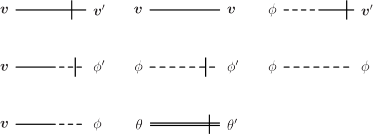
Figure 1: Graphical representation of all propagators of the model given by the quadratic part of the action (12).

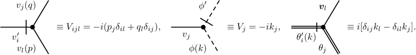
Figure 2: Graphical representation of all interaction vertices of the model given by the nonlinear part of the action (12).

3 Renormalization group analysis

Ultraviolet renormalizability reveals itself in a presence divergences in Feynman graphs, which are constructed according to simple laws [25, 28] using a graphical notation from Figs. 1 and 2. From a practical point of view, an analysis of the 1-particle irreducible Green functions, later referred to as 1-irreducible Green functions following the notation in [25], is of utmost importance. In the case of dynamical models [25, 28] two independent scales have to be introduced: the time scale $T$ and the length scale $L$. Thus the canonical dimension of any quantity $F$ (a field or a parameter) is described by two numbers, the frequency dimension $d_{F}^{\omega}$ and the momentum dimension $d_{F}^{k}$, defined such that

$$d_{k}^{k}=-d_{x}^{k}=1,\quad d_{k}^{\omega}=d_{x}^{\omega}=0,\quad d_{\omega}^{\omega}=-d_{t}^{\omega}=1,\quad d_{\omega}^{k}=d_{t}^{k}=0,$$ (16)

and the given quantity then scales as

$$[F]\sim[T]^{-d_{F}^{\omega}}[L]^{-d_{F}^{k}}.$$ (17)

The remaining dimensions can be found from the requirement that each term of the action functional (12) be dimensionless, with respect to both the momentum and the frequency dimensions separately.

Based on $d_{F}^{k}$ and $d_{F}^{\omega}$ the total canonical dimension $d_{F}=d_{F}^{k}+2d_{F}^{\omega}$ can be introduced, which in the renormalization theory of dynamic models plays the same role as the conventional (momentum) dimension does in static problems [25]. Setting $\omega\sim k^{2}$ ensures that all the viscosity and diffusion coefficients in the model are dimensionless. Another option is to set the speed of sound $c_{0}$ dimensionless and consequently obtain that $\omega\sim k$, i.e., $d_{F}=d_{F}^{k}+d_{F}^{\omega}$. This variant would mean that we are interested in the asymptotic behaviour of the Green functions as $\omega\sim k\to 0$, in other words, in sound modes in turbulent medium. Even though this problem is very interesting itself, it is not yet accessible for the RG treatment, so we do not discuss it here. The choice $\omega\sim k^{2}\to 0$ is the same as in the models of incompressible fluid, where it is the only possibility because the speed of sound is infinite. A similar alternative in dispersion laws exists, for example, within the so-called model H of equilibrium dynamical critical behaviour, see [25, 28].

The canonical dimensions for the velocity part of the model (13) are listed in Tab. 1, whereas parameters of the magnetic part are given in Tab. 2. From Tabs. 1 and 2 it follows that the model is logarithmic (the coupling constants $g_{10}\sim[L]^{-y}$ and $g_{20}\sim[L]^{-\varepsilon}$ become dimensionless) at $y=\varepsilon=0$. In this work we use the minimal subtraction (MS) scheme for the calculation of renormalization constants. In this scheme the UV divergences in the Green functions manifest themselves as poles in $y$, $\varepsilon$ and their linear combinations. Here, in accordance with critical phenomena we retain the notation $\varepsilon=4-d$ .

Table 1: Canonical dimensions of the fields and parameters entering velocity part of the total action (13).

$F$	$v_{i}^{\prime}$	$v_{i}$	$\phi^{\prime}$	$\phi$	$m$, $\mu$, $\Lambda$	$\nu_{0}$, $\nu$	$c_{0}$, $c$	$g_{10}$	$g_{20}$	$u_{0}$, $v_{0}$ $w_{0}$, $u$, $v$, $g_{1}$, $g_{2}$, $\alpha$
$d_{F}^{k}$	$d+1$	$-1$	$d+2$	$-2$	1	$-2$	$-1$	$y$	$4-d$	0
$d_{F}^{\omega}$	$-1$	1	$-2$	2	0	1	1	0	0	0
$d_{F}$	$d-1$	1	$d-2$	2	1	0	1	$y$	$4-d$	0

Table 2: Canonical dimensions of the fields and parameters entering magnetic part of the total action (14).

$F$	$\theta^{\prime}$	$\theta$	$\kappa$, $\kappa_{0}$	$w_{0}$, $w$
$d_{F}^{k}$	$d$	0	$-2$	0
$d_{F}^{\omega}$	$1/2$	$-1/2$	1	0
$d_{F}$	$d+1$	$-1$	1	0

The total canonical dimension of any 1-irreducible Green function $\Gamma$ is given by the relation

$$\delta_{\Gamma}=d+2-\sum_{\Phi}N_{\Phi}d_{\Phi},$$ (18)

where $N_{\Phi}$ is the number of the given type of field entering the function $\Gamma$, $d_{\Phi}$ is the corresponding total canonical dimension of field $\Phi$, and the summation runs over all types of the fields $\Phi$ in function $\Gamma$ [25, 26, 28].

Superficial UV divergences whose removal requires counterterms can be present only in those functions $\Gamma$ for which the formal index of divergence $\delta_{\Gamma}$ is a non-negative integer. A dimensional analysis should be augmented by the several additional considerations. They are clearly stated in the previous work [45, 52]. Therefore, we do not repeat them here and continue with a simple conclusion that model with the action (12) is renormalizable. The only graphs that are needed to be calculated are two-point Green functions. For a velocity part, the following graphs have to be analyzed

(19)

and for a magnetic part we have one Feynman diagram

$$\raisebox{-4.30554pt}{ \includegraphics[width=99.58464pt]{ThTh.pdf}}.$$ (20)

The remaining diagrams are either UV finite or the Galilean invariance prohibits their presence. Because the calculation of the divergent parts of Feynman diagrams is rather straightforward and proceeds in the usual fashion [25, 26, 28, 59], we refrain from mentioning here all the technical details. For the latter, we recommend an interested reader to consult our previous works [45, 50, 51, 52]. In what follows, we focus on important results that follows for the MHD model (14).

Here, we just provide a result of the diagram $D$ shown in Eq. (20)

$$D=\frac{\overline{S_{d}}}{2d}p^{2}P_{12}({\bm{p}})\nu \biggl{\{}\frac{1-d}{1+w}\biggl{[}\frac{g_{1}}{y}\biggl{(}\frac{\mu}{m}\biggl{)}^{y}+\frac{g_{2}}{\varepsilon}\biggl{(}\frac{\mu}{m}\biggl{)}^{\varepsilon}\biggl{]}$$

$${-\frac{u-w}{u(u+w)}\biggl{[}\frac{\alpha g_{1}}{y}\biggl{(}\frac{\mu}{m}\biggl{)}^{y}+\frac{g_{2}}{\varepsilon}\biggl{(}\frac{\mu}{m}\biggl{)}^{\varepsilon}\biggl{]}\biggl{\}}}$$ (21)

where $\overline{S_{d}}=S_{d}/(2\pi)^{d}$ with $S_{d}=2\pi^{d/2}/\Gamma(d/2)$ is the surface area of the unit sphere in the $d-$dimensional space and $\Gamma(x)$ is Euler’s Gamma function. The expression (21) differs from the result obtained in [45] by the presence of terms containing the charge $g_{2}$.

Further, from (21) we directly derive renormalization constant $Z_{\kappa}$ [where $\kappa=\nu w$, see Eq. (14)]

$$Z_{\kappa}=1-\frac{g_{1}}{2dwy}\biggl{[}\frac{d-1}{1+w}+\frac{\alpha(u-w)}{u(u+w)^{2}}\biggl{]}-\frac{g_{2}}{2dwy}\biggl{[}\frac{d-1}{1+w}+\frac{(u-w)}{u(u+w)^{2}}\biggl{]}$$ (22)

and the corresponding anomalous dimension

$$\gamma_{\kappa}=\frac{g_{1}}{2dwy}\biggl{[}\frac{d-1}{1+w}+\frac{\alpha(u-w)}{u(u+w)^{2}}\biggl{]}+\frac{g_{2}}{2dwy}\biggl{[}\frac{d-1}{1+w}+\frac{(u-w)}{u(u+w)^{2}}\biggl{]}.$$ (23)

4 Scaling regimes

The relation between the initial and renormalized action functionals $\mathcal{S}(\Phi,e_{0})=\mathcal{S}^{R}(Z_{\Phi}\Phi,e,\mu)$ (where $e_{0}$ is the complete set of bare parameters and $e$ is the set of their renormalized counterparts) yields the fundamental RG differential equation:

$$\biggl{\{}{\cal D}_{RG}+N_{\phi}\gamma_{\phi}+N_{\phi^{\prime}}\gamma_{\phi^{\prime}}\biggr{\}}\,G^{R}(e,\mu,\dots)=0,$$ (24)

where $G=\langle\Phi\cdots\Phi\rangle$ is a correlation function of the fields $\Phi$; $N_{\phi}$ and $N_{\phi^{\prime}}$ are the counts of normalization-requiring fields $\phi$ and $\phi^{\prime}$, respectively, which are the inputs to $G$; the ellipsis in expression (24) stands for the other arguments of $G$ (spatial and time variables, etc.). ${\cal D}_{RG}$ is the operation $\widetilde{\cal D}_{\mu}$ expressed in the renormalized variables and $\widetilde{\cal D}_{\mu}$ is the differential operation $\mu\partial_{\mu}$ for fixed $e_{0}$. For the present model it takes the form

$${\cal D}_{RG}={\cal D}_{\mu}+\beta_{g_{1}}\partial_{g_{1}}+\beta_{g_{2}}\partial_{g_{2}}+\beta_{u}\partial_{u}+\beta_{v}\partial_{v}-\gamma_{\nu}{\cal D}_{\nu}-\gamma_{c}{\cal D}_{c}.$$ (25)

Here, we have denoted ${\cal D}_{x}\equiv x\partial_{x}$ for any variable $x$. The anomalous dimension $\gamma_{F}$ of some quantity $F$ (a field or a parameter) is defined as

$$\gamma_{F}=Z_{F}^{-1}\widetilde{\cal D}_{\mu}Z_{F}=\widetilde{\cal D}_{\mu}\ln Z_{F},$$ (26)

and the $\beta$ functions for the four dimensionless coupling constants $g_{1}$, $g_{2}$, $u$ and $v$, which express the flows of parameters under the RG transformation, are $\beta_{g}=\widetilde{\cal D}_{\mu}g$. This yields

$$\beta_{g_{1}} =g_{1}\,(-y-\gamma_{g_{1}}), \beta_{g_{2}} =g_{2}\,(-\varepsilon-\gamma_{g_{2}}), \beta_{u} =-u\gamma_{u},$$

$$\beta_{v} =-v\gamma_{v}, \beta_{w} =w(\gamma_{\nu}-\gamma_{\kappa}).$$ (27)

The last term follows from the introduced definition of the charge $w$ in Eq.(14). Based on the analysis of the RG equation (24) it follows that the large scale behaviour with respect to spatial and time scales is governed by the IR attractive (“stable”) fixed points $g^{*}\equiv\{g_{1}^{*},g_{2}^{*},u^{*},v^{*}\}$, whose coordinates are found from the conditions [25, 26, 59]:

$$\beta_{g_{1}}(g^{*})=\beta_{g_{2}}(g^{*})=\beta_{u}(g^{*})=\beta_{v}(g^{*})=0.$$ (28)

Let us consider a set of invariant couplings $\overline{g}_{i}=\overline{g}_{i}(s,g)$ with the initial data $\overline{g}_{i}|_{s=1}=g_{i}$. Here, $s=k/\mu$ and IR asymptotic behaviour (i.e., behaviour at large distances) corresponds to the limit $s\rightarrow 0$. An evolution of invariant couplings is described by the set of flow equations

$$\mathcal{D}_{s}\overline{g}_{i}=\beta_{i}(\overline{g}_{j}),$$ (29)

whose solution as $s\to 0$ behaves approximately like

$$\overline{g}_{i}(s,g^{*})\cong g^{*}+const\times s^{\omega_{i}},$$ (30)

where $\left\{\omega_{i}\right\}$ is the set of eigenvalues of the matrix

$$\Omega_{ij}=\partial\beta_{i}/\partial g_{j}|_{g=g_{*}}.$$ (31)

The existence of IR attractive solutions of the RG equations leads to the existence of the scaling behaviour of Green functions. From (30) it follows that the type of the fixed point is determined by the matrix (31): for the IR attractive fixed points the matrix $\Omega$ has to be positive definite.

The character of the IR behaviour depends on the mutual relation between $y$ and $\varepsilon$ – two formally small quantities which were introduced in the correlator of the random force in the Navier-Stokes equation. In practical calculations they constitute parameters into which universal quantities are expanded. This is done in a similar fashion as calculation of critical exponents in $\phi^{4}$ theory, see [25, 26, 27, 28].

In work [52] the velocity part (without $\beta_{w}$) of the system (27) was analyzed. Altogether three IR attractive fixed points, which defines possible scaling regimes of the system, were found. The fixed point FPI (the trivial or Gaussian point) is stable if $y$, $\varepsilon<0$. The coordinates are

$$g_{1}^{*}=0,\quad g_{2}^{*}=0.$$ (32)

The fixed point FPII, which is stable if $\varepsilon>0$ and $y<3\varepsilon/2$, has the following coordinates

$$g_{1}^{*}=0,\quad g_{2}^{*}=\frac{8\varepsilon}{3}.$$ (33)

The fixed point FPIII (stable if $y>0$ and $y>3\varepsilon/2$) is

$$g_{1}^{*}=\frac{16y(2y-3\varepsilon)}{9[y(2+\alpha)-3\varepsilon]},\quad g_{2}^{*}=\frac{16\alpha y^{2}}{9[y(2+\alpha)-3\varepsilon]}.$$ (34)

The crossover between the two nontrivial points (33) and (34) takes place across the line $y=3\varepsilon/2$, which is in accordance with results of [37].

Moreover, from the analysis in [52] it follows that for nontrivial regimes the coordinate $u$ takes value $u^{*}=1$. Substituting these values together with $d=4$ we obtain for the charge $w$ the following beta function

$$\beta_{w}=\frac{w-1}{16(1+w)^{2}}\biggl{[}g_{1}(6+2\alpha+9w+3w^{2})+g_{2}(3w^{2}+9w+8)\biggl{]}.$$ (35)

Note that this result is in accordance with previous work for the passive scalar case [51] and vector case as well [61]. The expression in the square brackets in Eq. (35) is always positive for physically permissible values, i.e., $g_{1}>0,g_{2}>0,w>0$ and $\alpha>0$. Therefore, only one nontrivial solution for the fixed point exists, $w^{*}=1$. Also it is rather straightforward to show that $\partial_{w}\beta_{w}>0$ at nontrivial fixed points, what ensures IR stability.

Depending on the values of $y$ and $\varepsilon$, the different values of the critical dimension for various quantities $F$ are obtained. They can be calculated via the expression

$$\Delta[F]=d^{k}_{F}+\Delta_{\omega}d^{\omega}_{F}+\gamma_{F}^{*},$$ (36)

where $d^{\omega}_{F}$ is the canonical frequency dimension, $d^{k}_{F}$ is the momentum dimension, $\gamma_{F}^{*}$ is the anomalous dimension at the critical point (FPII or FPIII), and $\Delta_{\omega}=2-\gamma_{\nu}^{*}$ is the critical dimension of frequency.

Using Eq. (36) the critical dimension of the passive scalar density field $\theta$ and the field $\theta^{\prime}$ were obtained for the fixed points FPII and FPIII:

$$\Delta_{\theta_{i}} =-1+\varepsilon/4,\quad\Delta_{\theta_{i}^{\prime}}=d+1-\varepsilon/4\quad\text{for the fixed point FP${\textrm{II}}$};$$ (37)

$$\Delta_{\theta_{i}} =-1+y/6,\quad\Delta_{\theta_{i}^{\prime}}=d+1-y/6\quad\text{for the fixed point FP${\textrm{III}}$}.$$ (38)

Measurable quantities are some correlation functions or structure functions of composite operators. A local composite operator is a monomial or polynomial constructed from the primary fields $\theta(x)$ and their finite-order derivatives at a single space-time point $x$. In the Green functions with such objects, new UV divergences arise due to the coincidence of the field arguments. They can be removed by the additional renormalization procedure [25, 62].

The simplest case of a composite operator is the scalar operator $F(x)=\theta^{n}(x)$. Here, we focus on the irreducible tensor operators of the form

$$F^{(n,l)}_{i_{1}\dots i_{l}}=\theta_{i_{1}}\cdots\theta_{i_{l}}\,(\theta_{j}\theta_{j})^{s}+\dots,$$ (39)

where $l$ is the number of the free vector indices (the rank of the tensor) and $n=l+2s$ is the total number of the fields $\theta$ entering the operator. The ellipsis stands for the subtractions with the Kronecker’s delta symbols that make the operator irreducible (so that a contraction with respect to any pair of the free tensor indices vanish). For instance,

$$F^{(2,2)}_{ij}=\theta_{i}\theta_{j}-\frac{\delta_{ij}}{d}\,(\theta_{k}\theta_{k}).$$ (40)

For practical calculations, it is convenient to contract the tensors (39) with an arbitrary constant vector $\lambda$$=\{\lambda_{i}\}$. The resulting scalar operator takes the form

$$F^{(n,l)}=(\lambda_{i}w_{i})^{l}(w_{i}w_{i})^{s}+\dots,\quad w_{i}\equiv\partial_{i}\theta,$$ (41)

where the subtractions, denoted by the ellipsis, necessarily include the factors of $\lambda^{2}=\lambda_{i}\lambda_{i}$.

In order to calculate the critical dimension of the operator, one has to renormalize it. The operators (39) can be treated as multiplicatively renormalizable, $F^{(n,l)}=Z_{(n,l)}F^{(n,l)}_{R}$, with certain renormalization constants $Z_{(n,l)}$ (see [44]). The counterterm to $F^{(n,l)}$ must have the same rank as the operator itself. It means that the terms containing $\lambda^{2}$ should be excluded since the contracted fields $w_{i}w_{i}$, standing near them, reduce the number of free indices. It is sufficient to retain only the principal monomial, explicitly shown in (41), and to discard in the result all the terms with factors of $\lambda^{2}$. The renormalization constants $Z_{(n,l)}$ are determined by the finiteness of the 1-irreducible Green function $\Gamma_{nl}(x;\theta)$, which in the one-loop approximation is diagrammatically represented as

$$\Gamma_{nl}(x;\theta)=F^{(n,l)}+\frac{1}{2}\raisebox{-17.22217pt}{ \includegraphics[width=34.14322pt]{comp.pdf}},$$ (42)

where numerical factor $1/2$ is a symmetry factor of the graph and the thick dot with two lines attached denotes the operator vertex

$$V(x;x_{1},x_{2})=\frac{\delta^{2}F^{(n,l)}}{\delta\theta_{i}\delta\theta_{j}}.$$ (43)

Divergent parf of a one-loop diagram in (Eq. 42) reads

$$=-\frac{F_{nl}}{2wd(d+2)}\biggl{[}\frac{Q_{1}}{(1+w)}\biggl{(}\frac{g_{1}}{y}+\frac{g_{2}}{\varepsilon}\biggl{)}+\frac{Q_{2}}{u(u+w)}\biggl{(}\frac{\alpha g_{1}}{y}+\frac{g_{2}}{\varepsilon}\biggl{)}\biggl{]};$$

$$Q_{1} \equiv-n(n+d)(d-1)-l(d+1)(d+l-2),$$

$$Q_{2} \equiv-n(d-1)(nd+n-d)-l(d+l-2).$$

The expressions for the propagators and vertices at the bottom of the diagram can be found in [52]. Then using the chain rule and up to irrelevant terms the vertex (43) for the operator $F^{(n,l)}$ can be presented in the form

$$V(x;x_{1},x_{2})=\frac{\partial^{2}F^{(n,l)}}{\partial w_{i}\partial w_{j}}\,\delta(x-x_{1})\,\delta(x-x_{2}).$$ (44)

The differentiation yields

$${\partial^{2}F^{(n,l)}}/{\partial w_{i}\partial w_{j}} =2s(w^{2})^{s-2}(\lambda w)^{l}\left[\delta_{ij}w^{2}+2(s-1)w_{i}w_{j}\right]+l(l-1)(w^{2})^{s}$$

$$\times(\lambda w)^{l-2}\lambda_{i}\lambda_{j}++2ls(w^{2})^{s-1}(\lambda w)^{l-1}(w_{i}\lambda_{j}+w_{j}\lambda_{i}),$$ (45)

where $w^{2}=w_{k}w_{k}$, $(\lambda w)=\lambda_{k}w_{k}$ and substitution $w_{i}\rightarrow\theta_{i}$ is assumed. Two more factors $w_{p}w_{r}$ are attached to the bottom of the diagram due to the derivatives coming from the vertices $\theta^{\prime}_{i}(v_{k}\partial_{k})\theta_{i}$. The ultraviolet divergence is logarithmic and one can set all the external frequencies and momenta equal to zero; then the core of the diagram takes the form

$$\int\frac{\text{d}\omega}{2\pi}\int_{k>m}\frac{{{\mathrm{d}}^{d}}{k}}{(2\pi)^{d}}\,k_{i}k_{j}\,D_{pr}(\omega,{{\bm{k}}})\,\frac{1}{\omega^{2}+w^{2}\nu^{2}k^{4}}.$$ (46)

Here the first factor comes from the derivatives in (43), $w=\kappa/\nu$, $D_{pr}$ is the velocity correlation function [see (5)], and the last factor comes from the two propagators $\langle\theta^{\prime}\theta\rangle_{0}$.

After the integration, combining all the factors, contracting the tensor indices and expressing the result in terms of $n=l+2s$ and $l$, one obtains:

$$\Gamma_{n}(x;\theta) =F^{(n,l)}(x)\,\biggl{\{}1-\frac{1}{4wd(d+2)}\,\biggl{[}\frac{Q_{1}}{(1+w)}\biggl{(}\frac{g_{1}}{y}+\frac{g_{2}}{\varepsilon}\biggl{)}$$

$$+\frac{Q_{2}}{u(u+w)}\biggl{(}\frac{\alpha g_{1}}{y}+\frac{g_{2}}{\varepsilon}\biggl{)}\biggl{]}\biggl{\}}.$$ (47)

Then the renormalization constants $Z_{(n,l)}$ calculated in the MS scheme read

$$Z_{(n,l)}=1-\frac{1}{4dw(d+2)}\,\left[\frac{Q_{1}}{1+w}\left(\frac{g_{1}}{y}+\frac{g_{2}}{\varepsilon}\right)+\frac{Q_{2}}{u(u+w)}\left(\frac{\alpha g_{1}}{y}+\frac{g_{2}}{\varepsilon}\right)\right].$$ (48)

For the corresponding anomalous dimension one obtains

$$\gamma_{(n,l)}=\frac{1}{4dw(d+2)}\,\left\{\frac{Q_{1}}{1+w}(g_{1}+g_{2})+\frac{Q_{2}}{u(u+w)}(\alpha g_{1}+g_{2})\right\}.$$ (49)

In order to evaluate the critical dimension, one needs to substitute the coordinates of the fixed points into the expression (49) and then use the relation (36). For the fixed point FPII the critical dimension is

$$\Delta_{(n,l)}=\frac{n}{4}\varepsilon+\frac{Q_{1}+Q_{2}}{72}\varepsilon.$$ (50)

For the fixed point FPIII it is

$$\Delta_{(n,l)}=\frac{n}{6}y+\frac{y}{12}\frac{Q_{1}(\alpha y+2y-3\varepsilon)+3\alpha Q_{2}(y-\varepsilon)}{9[y(2+\alpha)-3\varepsilon]}.$$ (51)

Both expressions (50) and (51) suppose higher order corrections in $y$ and $\varepsilon$.

Therefore, the infinite set of operators with negative critical dimensions, whose spectra is unbounded from below, is observed.

5 Operator Product Expansion

Our main interest are pair correlation functions, whose unrenormalized counterparts have been defined in Eq. (39). For Galilean invariant equal-time functions we can write the following representation

$$\langle F^{(m,i)}(t,{\bm{x}})F^{(n,j)}(t,{\bm{x}}^{\prime})\rangle\simeq\mu^{d_{F}}\nu^{d^{\omega}_{F}}(\mu r)^{-\Delta_{(m,i)}-\Delta_{(n,j)}}\zeta_{m,i;n,j}(mr,c(r)),$$ (52)

where $r=|{\bm{x}}-{\bm{x}}^{\prime}|$ and $c(r)$ is effective speed of sound. Its limiting behaviour can be shown [52] to be

$$c(r)=c\frac{(\mu r)^{\Delta_{c}}}{\mu\nu}\rightarrow\begin{cases}c(0)\quad\text{{for} non-local r;}\\ c(\infty)\quad\text{{for} local r.}\end{cases}$$

Eq. (52) is valid in the asymptotic limit $\mu r\gg 1$. Further, the inertial-convective range corresponds to the additional restriction $mr\ll 1$. The behaviour of the functions $\zeta$ at $mr\to 0$ can be studied by means of the OPE technique [25, 62]. The basic idea of this method is to represent a product of two operators at two close points, ${\bm{x}}$ and ${\bm{x}}^{\prime}$ with ${\bm{x}}-{\bm{x}}^{\prime}\rightarrow 0$, in the form

$$F^{(m,i)}(t,{\bm{x}})F^{(n,j)}(t,{\bm{x}}^{\prime})\simeq\sum_{F}C_{F}(mr)\,F\biggl{(}t,\frac{{\bm{x}}+{\bm{x}}^{\prime}}{2}\biggl{)},$$ (53)

where functions $C_{F}$ are regular in their argument and a given sum runs over all permissible local composite operators $F$ allowed by RG and symmetry considerations. Taken into account (52) and (53) in the limit $mr\rightarrow 0$ we arrive at the relation

$$\zeta(mr)\approx\sum_{F}A_{F}(mr)(mr)^{\Delta_{F}}$$

Considering OPE for the correlation functions $\langle F^{(p,0)}F^{(k,0)}\rangle$ with $n=p+k$, where $F^{(n,l)}$ is the operator of the type (39), one can observe that the leading contribution to the expansion is determined by the operator $F^{(n,0)}$ from the same family. Therefore, in the inertial range these correlation functions acquire the form

$$\langle F^{(p,0)}(t,{{\bm{x}}})F^{(k,0)}(t,{{\bm{x}}^{\prime}})\rangle\sim r^{-\Delta_{(p,0)}-\Delta_{(k,0)}+\Delta_{(n,0)}}.$$ (54)

The inequality $\Delta_{(n,0)}<\Delta_{(p,0)}+\Delta_{(k,0)}$, which follows from both explicit one-loop expressions (50) and (51), indicates, that the operators $F^{(n,0)}$ demonstrate a “multifractal” behaviour; see [63].

A direct substitution of $d=4$ leads to the following prediction for a critical dimension

$$\Delta_{n,l}=n\Delta_{\theta}+\gamma^{*}_{nl}=\begin{cases}-n+\frac{n\varepsilon}{4}+\frac{(Q_{1}+Q_{2})\varepsilon}{4}\qquad\text{for FPII}\\ -n+\frac{ny}{6}+\frac{Q_{1}y}{108}+\frac{Q_{2}\alpha y(y-\varepsilon)}{36[y(2+\alpha)-3\varepsilon]}\qquad\text{for FPIII}\end{cases}$$ (55)

where we have

$$Q_{1}|_{d=4}=-3n(n+4)+5l(2+l),\quad Q_{2}|_{d=4}=-3n(5n-4)+l(2+l).$$

From these results several observations can be made. Based on (55) we see that for fixed $n$ kind of a hierarchy present with respect to the index $l$, i.e,

$$\frac{\partial\Delta_{n,l}}{\partial l}>0.$$ (56)

In other words, the higher $l$ the less important contribution. The most relevant is given by the isotropic shell with $l=0$. This is in accordance with previous studies [61, 44, 45]. Moreover, we observe that there is no appearance of the parameter $\alpha$ for the local regime FPII. Further, in contrast to [45] there is no monotonous behaviour in $\alpha$ of $\Delta_{n0}$ for the non-local regime.

6 Conclusion

In the present paper the advection of the vector field by the Navier-Stokes velocity ensemble has been examined. The fluid was assumed to be compressible and the space dimension was close to $d=4$. The problem has been investigated by means of renormalization group and operator product expansion; the double expansion in $y$ and $\varepsilon=4-d$ was constructed.

There are two nontrivial IR stable fixed points in this model and, therefore, the critical behaviour in the inertial range demonstrates two different regimes depending on the relation between the exponents $y$ and $\varepsilon$. The expressions for the critical exponents of the vector field $\theta$ were obtained in the leading one-loop approximation.

In order to find the anomalous exponents of the structure functions, the composite fields (39) were renormalized. The critical dimensions of them were evaluated. It turned out that there is an infinite number of the dangerous operators, i.e., the operators with negative critical dimensions. Besides, OPE allowed us to derive the explicit expressions for the critical dimensions of the structure functions. The existence of the anomalous scaling in the inertial-convective range was established for both possible scaling regimes. Another very interesting result is that some kinds of operators exhibit the “multifractal” behaviour.

With regard to future research, it would be interesting to go beyond the one-loop approximation and to analyze the behaviour more precisely on the higher level of accuracy. Another very important task to be further investigated is to have a closer look at the both scalar and vector active fields, i.e., to consider a back influence of the advected fields to the turbulent environment flow.

References

- [1] U. Frisch, Turbulence: The Legacy of A. N. Kolmogorov (Cambridge University Press, Cambridge, 1995).
- [2] P. A. Davidson, Turbulence: an introduction for scientists and engineers (2th edition, Oxford University Press, Oxford, 2015).
- [3] S. N. Shore, Astrophysical Hydrodynamics:An Introduction (Wiley-VCH Verlag GmbH& KGaA, Weinheim, 2007).
- [4] E. Priest, Magnetohydrodynamics of the sun (Cambridge University Press, 2014).
- [5] N. V. Antonov, J. Phys. A: Math. Gen. 39, 7825 (2006).
- [6] H. K. Moffatt, Magnetic field generation in electrically conducting fluids (Cambridge University Press, Cambridge 1978).
- [7] J. D. Fournier, P. L. Sulem, A. Pouquet, J. Phys. A 15, 1393 (1982).
- [8] L. Ts. Adzhemyan, A. N. Vasil’ev, and M. Gnatich, Theor. Math. Phys. 64(2), 777 (1985).
- [9] J. Kim, and D. Ryu, Astrophys. J. 630, L45 (2005).
- [10] V. Carbone, R. Marino, L. Sorriso-Valvo, A. Noullez, and R. Bruno, Phys. Rev. Lett. 103, 061102 (2009).
- [11] F. Sahraoui, M. L. Goldstein, P. Robert, Yu. V. Khotyainstsev, Phys. Rev. Lett. 102, 231102 (2009).
- [12] H. Aluie, and G. L. Eyink, Phys. Rev. Lett. 104, 081101 (2010).
- [13] S. Galtier, and S. Banerjee, Phys. Rev. Lett. 107, 134501 (2011).
- [14] S. Banerjee, and S. Galtier, Phys. Rev. E 87, 013019 (2013).
- [15] S. Banerjee, L. Z. Hadid, F. Sahraoui, and S. Galtier, Astrophys. J. Lett. 829, L27, (2016).
- [16] L. Z. Hadid, F. Sahraoui, and S. Galtier, Astrophys. J. 838, 9 (2017).
- [17] L. D. Landau and E. M. Lifshitz, Fluid Mechanics (Pergamon Press, Oxford, 1959).
- [18] P. Sagaut, C. Cambon, Homogeneous Turbulence Dynamics (Cambridge University Press, 2008).
- [19] P. S. Iroshnikov, Sov. Astron. 7, 566 (1964).
-
[20]
N. V. Antonov and N. M. Gulitskiy, Lecture Notes in Comp. Science,
7125/2012, 128 (2012);
N. V. Antonov and N. M. Gulitskiy, Phys. Rev. E 85, 065301(R) (2012);
N. V. Antonov and N. M. Gulitskiy, Phys. Rev. E 87, 039902(E) (2013). -
[21]
E. Jurčišinova and M. Jurčišin, J. Phys. A: Math. Theor., 45, 485501 (2012);
E. Jurčišinova and M. Jurčišin, Phys. Rev. E 88, 011004 (2013). -
[22]
E. Jurčišinova and M. Jurčišin, Phys. Rev. E 77, 016306 (2008);
E. Jurčišinova, M. Jurčišin and R. Remecky, Phys. Rev. E 80, 046302 (2009);
E. Jurčišinova, M. Jurčišin and R. Remecky, J. Phys. A: Math. Theor. 42, 275501 (2009). -
[23]
N. V. Antonov and N. M. Gulitskiy, Phys. Rev. E 91, 013002 (2015);
N. V. Antonov and N. M. Gulitskiy, Phys. Rev. E 92, 043018 (2015);
N. V. Antonov and N. M. Gulitskiy, AIP Conf. Proc. 1701, 100006 (2016);
N. V. Antonov and N. M. Gulitskiy, EPJ Web of Conf. 108, 02008 (2016). - [24] G. Falkovich, K. Gawȩdzki and M. Vergassola, Rev. Mod. Phys. 73, 913 (2001).
- [25] A. N. Vasil’ev, The Field Theoretic Renormalization Group in Critical Behavior Theory and Stochastic Dynamics (Boca Raton, Chapman Hall/CRC, 2004).
- [26] J. Zinn-Justin, Quantum Field Theory and Critical Phenomena (4th edition, Oxford University Press, Oxford, 2002).
- [27] L. Ts. Adzhemyan, N. V. Antonov, A. N. Vasil’ev: The Field Theoretic Renormalization Group in Fully Developed Turbulence (Gordon & Breach, London, 1999).
- [28] U. Täuber, Critical Dynamics: A Field Theory Approach to Equilibrium and Non-Equilibrium Scaling Behavior (Cambridge University Press, New York, 2014).
- [29] R.H. Kraichnan, Phys. Fluids 11, 945 (1968).
-
[30]
K. Gawȩdzki and A. Kupiainen, Phys. Rev. Lett. 75, 3834 (1995);
D. Bernard, K. Gawȩdzki, and A. Kupiainen, Phys. Rev. E 54, 2564 (1996);
M. Chertkov and G. Falkovich, Phys. Rev. Lett. 76, 2706 (1996) - [31] L. Ts. Adzhemyan, N. V. Antonov, and A. N. Vasil’ev, Phys. Rev. E 58, 1823 (1998).
- [32] E. Jurčišinova and M. Jurčišin, Phys. Rev. E 91, 063009 (2015).
-
[33]
N. V. Antonov, A. Lanotte, and A. Mazzino, Phys. Rev. E 61, 6586 (2000);
N. V. Antonov and N. M. Gulitskiy, Theor. Math. Phys., 176(1), 851 (2013). - [34] H. Arponen, Phys. Rev. E, 79, 056303 (2009).
- [35] M. Hnatič, J. Honkonen, T. Lučivjanský, Acta Physica Slovaca 66, 69 (2016).
- [36] L. Ts. Adzhemyan, N. V. Antonov, J. Honkonen, and T. L. Kim, Phys. Rev. E 71, 016303 (2005).
- [37] N. V. Antonov, Phys. Rev. Lett. 92, 161101 (2004).
- [38] N. V. Antonov, N. M. Gulitskiy, and A. V. Malyshev, EPJ Web of Conf. 126, 04019 (2016).
- [39] E. Jurčišinova, M. Jurčišin, R. Remecky, Phys. Rev. E 93, 033106 (2016).
- [40] M. Vergassola and A. Mazzino, Phys. Rev. Lett. 79, 1849 (1997).
- [41] A. Celani, A. Lanotte, and A. Mazzino, Phys. Rev. E 60 R1138 (1999).
- [42] M. Chertkov, I. Kolokolov, and M. Vergassola, Phys. Rev. E. 56, 5483 (1997).
- [43] N. V. Antonov, M. Yu. Nalimov and A. A. Udalov, Theor. Math. Phys. 110, 305 (1997).
- [44] N. V. Antonov and M. M. Kostenko, Phys. Rev. E 90, 063016 (2014).
- [45] N. V. Antonov and M. M. Kostenko, Phys. Rev. E 92, 053013 (2015).
- [46] M. Hnatich, E. Jurčišinova, M. Jurčišin, and M. Repašan, J. Phys. A: Math. Gen. 39, 8007 (2006).
- [47] V. S. L’vov and A. V. Mikhailov, Preprint No. 54, Inst. Avtomat. Electron., Novosibirsk (1977).
- [48] I. Staroselsky, V. Yakhot, S. Kida, and S. A. Orszag, Phys. Rev. Lett., 65, 171 (1990).
- [49] S. S. Moiseev, A. V. Tur, and V. V. Yanovskii, Sov. Phys. JETP 44, 556 (1976).
- [50] N.V. Antonov, N. M. Gulitskiy, M. M. Kostenko, T. Lučivjanský, EPJ Web of Conf. 125, 05006 (2016).
- [51] N.V. Antonov, N. M. Gulitskiy, M. M. Kostenko, T. Lučivjanský, EPJ Web of Conf. 137, 10003 (2016).
- [52] N.V. Antonov, N. M. Gulitskiy, M. M. Kostenko, T. Lučivjanský, Phys. Rev. E 95, 0331200 (2017).
- [53] A. Z. Patashinskii, V. L. Pokrovskii, Fluctuation Theory of Phase Transitions (Pergamon Press, Oxford, 1979).
- [54] L. Ts. Adzhemyan, N. V. Antonov, and A. N. Vasil’ev, Sov. Phys. JETP 68, 733 (1989).
- [55] J. Honkonen and M. Yu. Nalimov, Z. Phys. B 99, 297 (1996).
- [56] L. Ts. Adzhemyan, J. Honkonen, M. V. Kompaniets, A. N. Vasil’ev, Phys. Rev. E 71(3), 036305 (2005).
- [57] L. Ts. Adzhemyan, M. Hnatich and J. Honkonen, Eur. Phys. J B 73, 275 (2010).
- [58] N. .V. Antonov, A. Lanotte, and A. Mazzino, Phys. Rev. E 61, 6586 (2000).
- [59] D. J. Amit and V. Martín-Mayor, Field Theory, the Renormalization Group and Critical Phenomena (World Scientific,Singapore,2005).
- [60] D. Yu. Volchenkov and M. Yu. Nalimov, Theor. Math. Phys. 106(3), 307 (1996).
- [61] N. V. Antonov, M. Hnatich, J. Honkonen, and M. Jurčišin, Phys. Rev. E 68, 046306 (2003).
- [62] J. C. Collins, Renormalization: an Introduction to Renormalization, the Renormalization Group , and the Operator-Product Expansion (Cambridge University Press, Cambridge, 1984).
-
[63]
B. Duplantier and A. Ludwig, Phys. Rev. Lett. 66, 247 (1991);
G. L. Eyink, Phys. Lett. A 172, 355 (1993).