Energy transfer mechanisms in a dipole chain: From energy equipartition to the formation of breathers

Abstract

We study the energy transfer in a classical dipole chain of $N$ interacting rigid rotating dipoles. The underlying high–dimensional potential energy landscape is analyzed in particular by determining the equilibrium points and their stability in the common plane of rotation. Starting from the minimal energy configuration, the response of the chain to excitation of a single dipole is investigated. Using both the linearized and the exact Hamiltonian of the dipole chain, we detect an approximate excitation energy threshold between a weakly and a strongly nonlinear dynamics. In the weakly nonlinear regime, the chain approaches in the course of time the expected energy equipartition among the dipoles. For excitations of higher energy, strongly localized excitations appear whose trajectories in time are either periodic or irregular, relating to the well-known discrete or chaotic breathers, respectively. The phenomenon of spontaneous formation of domains of opposite polarization and phase locking is found to commonly accompany the time evolution of the chaotic breathers. Finally, the sensitivity of the dipole chain dynamics to the initial conditions is studied as a function of the initial excitation energy by computing a fast chaos indicator. The results of this study confirm the aforementioned approximate threshold value for the initial excitation energy, below which the dynamics of the dipole chain is regular and above which it is chaotic.

I Introduction

The first numerical study of the energy transport in a one-dimensional (1D) nonlinear oscillator chain, known as the Fermi-Pasta-Ulam (FPU) model FPU ; A780 ; lady has been performed already in nineteen fifty five. The results of this numerical experiment were found to contradict the reasonable assumption that in the presence of a non-linear coupling between the oscillators the system would thermalize, i.e. an initial excitation of a single mode of the system would become equally distributed between all the modes of the chain. In particular, the numerical results showed a persistent recurrence of the energy to the initially excited mode, preventing the system from reaching equipartition up to long times. It has been soon realized that the origin of such a behavior were the nonlinear interaction terms, a fact that established the study of the energy exchange in discrete nonlinear lattices of oscillators as an active field of research in few- and many-body dynamics, see for instance Refs. Ford ; A897 ; A780 ; A842 ; Gallavotti ; Mussot ; Bambusi ; penati . Most attention has been paid to 1D oscillator chains with a cubic or quartic nonlinear coupling, the so-called FPU-$\alpha$ and FPU-$\beta$ models, respectively, A780 . Already studies of the energy transfer in these simple FPU models have provided interesting results, such as the existence of thresholds for stochasticity and therefore for equipartition A842 ; A899 ; A782 , as well as the discovery of phenomena of energy localization in discrete A866 ; A867 ; A868 or chaotic breathers A867 ; A851 ; A837 .

Beyond the theoretical FPU-like models, the mechanism of energy exchange is an important subject of investigation in microscopic systems such as molecules, interacting via Coulomb, dipole-dipole or van-der-Waals interactions. These fundamental interactions appear in different research disciplines including physics, chemistry, biology and material sciences, with applications covering such diverse topics as the photosynthesis of plants and bacteria van ; engel ; fotosintesis ; wu ; Burghard , the emission of light of organic materials Saikin ; Melnikau ; Qiao , molecular crystals Davydov ; Silbey ; Wright or artificial molecular rotors A829 . Moreover the advances in current technology have allowed the trapping and confinement of cold molecules in optical lattices where the positions of the molecules are fixed and their mutual interactions (e.g. dipole–dipole) usually masked by thermal fluctuation, become prominent krems ; weidemuller . Along these lines polar diatomic molecules trapped in optical lattices, exhibit due to their strong dipole-dipole interaction a particularly interesting quantum many-body behavior leading to novel structures and collective dynamics A753 ; rey ; Lewenstein .

Within the framework of classical mechanics, confined polar diatomic molecules can be considered as lattices of rigid dipoles. Following this approach, Ratner and co-workers Ratner1 ; Ratner2 ; Ratner3 have studied the energy transfer in chains of interacting rotating rigid dipoles in various planar configurations. Already the simplest two–dipole chain, recently revisited in PRE2017 , was found to display a rich dynamical behavior with a complicated phase space. Increasing the number of dipoles the energy transfer was shown to yield the formation of solitons or the emergence of chaoticity  A898 .

The objective of this paper is to provide further insights in the energy transfer mechanisms of a 1D chain of rotating classical dipoles. In such a chain the dipoles are assumed to be fixed in space, interacting through nearest neighbor (NN) interactions and rotating in a common plane. The interaction potential of even this simplified rigid-rotor model is found to be quite complex, supporting various equilibrium points including a minimum, a maximum and different saddle points. Considering the system in its ground state (GS) configuration (minimum) with a single dipole excited initially possesing a certain amount of kinetic energy we study the transport of the excess energy. We find that for increasing excess energy the degree of chaoticity of the energy transfer increases, passing through a weakly nonlinear and a highly nonlinear regime. Although in the former regime after some time the energy is almost equally partitioned among the dipoles of the chain, for high enough excitation energies the energy diffusion is prohibited, giving place to different energy localization patterns dictated by a strong nonlinearity. Among those patterns we can distinguish cases in which two domain walls, separating domains of dipoles with different polarization, are formed spontaneously and move irregularly in time. It turns out that the emergence of such patterns can be linked to the lowest energy saddle point of the interaction potential of the dipole chain. Moreover, for a large excitation energy, the dipole chain displays a strong sensitivity to the initial conditions, signifying its chaotic nature. We quantify the chaoticity of the system for different values of the excitation energy using a fast Lyapunov indicator.

The structure of the current paper is as follows. In Sec. II we present the Hamiltonian and the equations of motions of the dipole chain and discuss their equilibria. Linearizing these equations of motion around the GS, we arrive at the corresponding linear system whose properties are analyzed in Sec. III. The results for the energy transfer of a localized excitation are presented in Sec. IV and Sec. V. In particular, Sec. IV deals with the propagation of a low-energy excitation in the so-called weakly nonlinear regime, whereas Sec. V discusses the case of higher energy excitations in which the nonlinearity of the system is enhanced, leading to its chaotic behavior which is quantified by the Orthogonal Fast Lyapunov Indicator. Finally we provide our conclusions in Sec. VI.

II The Hamiltonian and the Equilibrium points

We consider a linear chain of $N$ identical rigid dipoles of electric dipole moment ${\bf d}_{i}=d\ {\bf u}_{i}$, which are fixed in space, separated by a constant distance $a_{l}$, and located along the $X$-axis of the Laboratory Fixed Frame (LFF) $XYZ$. The unit vectors ${\bf u}_{i}=(u_{xi},u_{yi},u_{zi})$ determine the orientation of each dipole subjected to the holonomic constraint $\left|{{\bf d}_{i}}\right|^{2}=d_{xi}^{2}+d_{yi}^{2}+d_{zi}^{2}=d^{2}$. The potential energy ${\cal V}_{ij}$ between each pair $(i,j)$ of rotors due to the mutual dipole-dipole interaction (DDI) is given by A753

$${\cal V}_{ij}=\frac{1}{4\pi\epsilon_{0}}\frac{({\bf d}_{i}\cdot{\bf d}_{j})\ r_{ij}^{2}-3\ ({\bf d}_{i}\cdot{\bf r}_{i,j})\ ({\bf d}_{j}\cdot{\bf r}_{i,j})}{r_{ij}^{5}}$$ ((1))

with ${\bf r}_{i}=\left(x_{i},y_{i}=0,z_{i}=0\right)$, ${\bf r}_{i,j}={\bf r}_{i}-{\bf r}_{j}$ and $r_{ij}=|{\bf r}_{i,j}|$.

Here we assume periodic boundary conditions (PBC) in the linear chain and we take into account only interactions between nearest neighbors (NN), the total interaction potential ${\cal V}$ of the system reads

$${\cal V}=\sum_{i=1}^{N}\ \frac{1}{4\pi\epsilon_{0}a_{l}^{5}}\bigg{[}({\bf d}_{i}\cdot{\bf d}_{i+1})\ a_{l}^{2}-3\ ({\bf d}_{i}\cdot{\bf r}_{i,i+1})\ ({\bf d}_{i+1}\cdot{\bf r}_{i,i+1})\bigg{]}.$$ ((2))

It is convenient to express the total interaction potential ${\cal V}$ in terms of the Euler angles $(0\leq\theta_{i}\leq\pi,0\leq\phi_{i}<2\pi)$ of each rotor, such that (2) takes the form

$${\cal V}(\theta_{i},\phi_{i})=\alpha\sum_{i=1}^{N}\bigg{[}\cos\theta_{i}\cos\theta_{i+1}+\sin\theta_{i}\sin\theta_{i+1}(\sin\phi_{i}\sin\phi_{i+1}-2\cos\phi_{i}\cos\phi_{i+1})\bigg{]},$$ ((3))

where $\alpha=d^{2}/4\pi\epsilon_{0}a_{l}^{3}$ is the strength of the DDI. Note that the well-known stable head-tail configurations of the dipoles appear at $\theta_{i}=\pm\pi/2$ and $\phi_{i}=0,\pi$. The rotational dynamics of the dipole chain is described by the Hamiltonian

$$H=\sum_{i=1}^{N}\frac{1}{2I}\bigg{[}p_{\theta_{i}}^{2}+\frac{p_{\phi_{i}}^{2}}{\sin^{2}\theta_{i}}\bigg{]}+{\cal V}(\theta_{i},\phi_{i}),$$ ((4))

where $I$ is the moment of inertia of each dipole. The Hamiltonian (4) defines a dynamical system with $2N$ degrees of freedom $\{(\theta_{i},p_{\theta_{i}}),(\phi_{i},p_{\phi_{i}})\}_{i=1}^{N}$ where $p_{\theta_{i}},p_{\phi_{i}}$ denote the conjugate momenta of $\theta_{i},\phi_{i}$ respectively. From the corresponding Hamiltonian equations of motion, it is easy to see that the manifold ${\cal M}$ of codimension $N$ given by

$${\cal M}=\{(\theta_{i},p_{\theta_{i}})\ |\ \phi_{i}=0,\pi\ \mbox{and}\ p_{\phi_{i}}=0\},$$ ((5))

is invariant under the dynamics. On this manifold, the number of degrees of freedom of the system reduces to $N$ and the Hamiltonian (4) becomes

$$H=\sum_{i=1}^{N}\frac{p_{\theta_{i}}^{2}}{2I}+\alpha\sum_{i=1}^{N}\bigg{[}\cos\theta_{i}\cos\theta_{i+1}-2\sin\theta_{i}\sin\theta_{i+1}\bigg{]},$$ ((6))

and the rotational motion of the dipoles is restricted to a given common polar plane of constant azimuthal inclination $\phi_{i}=0,\pi$ where the $N$ polar angles $\theta_{i}$ vary in the interval $[-\pi,\pi)$. From now on, we focus on the planar dynamics arising from the Hamiltonian (6). It is worth noticing that the Hamiltonian (6) is structurally stable in the sense that, for weak enough perturbations away from the manifold ${\cal M}$ and around the head-tail configuration, the dynamics takes place in the neighborhood of this configuration, which is the absolute minimum of the potential ${\cal V}(\theta_{i},\phi_{i})$.

As mentioned above the stable head-tail configurations of the dipoles in the manifold ${\cal M}$ appear for $\theta_{i}=\pm\pi/2$. For the sake of simplicity, we choose to move these equilibrium configurations to the origin $\theta_{i}=0$ and to $\theta_{i}=\pi$ respectively. To this end, we introduce the following canonical transformation between the previous $(\theta_{i},p_{\theta_{i}})$ and the new $(x_{i},p_{i})$ coordinates

$$x_{i}=\theta_{i}-\pi/2,\qquad p_{i}=p_{\theta_{i}}.$$ ((7))

Employing this transformation, the Hamiltonian (6) obtains the form

$$H=\sum_{i=1}^{N}\frac{p_{i}^{2}}{2I}+\alpha\sum_{i=1}^{N}\bigg{[}\sin x_{i}\sin x_{i+1}-2\cos x_{i}\cos x_{i+1}\bigg{]},$$ ((8))

where $p_{i}=I\ dx_{i}/dt$. Taking into account that our dipole chain model of Eq. (8) amounts essentially to the rigid rotor model used for the study of the dynamics of $N$ interacting polar diatomic molecules Ratner1 ; Ratner2 ; Ratner3 , we find it convenient to express the energy, i.e. the Hamiltonian (8), in units of the molecular rotational constant $B=\hbar^{2}/2I$. To this end we define a new dimensionless time $t^{\prime}=t/t_{B}$ with $t_{B}=\hbar/\sqrt{2}B$ whose use leads us to the following (dimensionless) Hamiltonian

$$E^{\prime}=\frac{H}{B}=\sum_{i=1}^{N}\frac{p_{i}^{\prime 2}}{2}+\chi\sum_{i=1}^{N}\bigg{[}\sin x_{i}\sin x_{i+1}-2\cos x_{i}\cos x_{i+1}\bigg{]},$$ ((9))

where $p_{i}^{\prime}=dx_{i}/dt^{\prime}$ and $\chi=\alpha/B$ is a dimensionless parameter controlling the dipole interaction. Besides the reduced energy $E^{\prime}=H/B$, the dynamics of the system described by (9) depends also on the dipole parameter $\chi$. However, this dependence can be removed by further rescaling the time, introducing $t^{\prime\prime}=\sqrt{\chi}\ t^{\prime}$. In terms of time $t^{\prime\prime}$, the Hamiltonian  (9) reads

$$E\equiv{\cal H}=\frac{H}{B\chi}=\sum_{i=1}^{N}\frac{p_{i}^{\prime\prime 2}}{2}+\sum_{i=1}^{N}\bigg{[}\sin x_{i}\sin x_{i+1}-2\cos x_{i}\cos x_{i+1}\bigg{]},$$ ((10))

where $p_{i}^{\prime\prime}=dx_{i}/dt^{\prime\prime}$, such that the dynamics only depends on the rescaled energy $E=H/B\chi$. The following study employs the Hamiltonian (10) and we omit the primes in order to simplify the notation.

We begin our exploration of the system’s dynamics by addressing first its static properties regarding its equilibria, i.e. the roots of the $N$-dimensional gradient (critical points) of the potential

$$V=\sum_{i=1}^{N}\bigg{[}\sin x_{i}\sin x_{i+1}-2\cos x_{i}\cos x_{i+1}\bigg{]},$$ ((11))

given by the system of equations ($\forall i=1,2,\ldots,N$)

$$\frac{\partial V}{\partial\theta_{i}}=\bigg{[}\cos x_{i}\sin x_{i+1}+2\sin x_{i}\cos x_{i+1}+\cos x_{i}\sin x_{i-1}+2\sin x_{i}\cos x_{i-1}\bigg{]}=0.$$ ((12))

II.1 Equilibrium points

From the inspection of Eqs. (12), we find the following critical points summarized in Fig. 1:

• The head-tail configuration of the dipoles $\{x_{i}=0,\forall i\}$ or $\{x_{i}=\pi,\forall i\}$ (Fig. 1 (i)). This critical point is a minimum of the potential (11) (see Appendix A) with energy $E_{m}=-2N.$ For the sake of simplicity, in the following we shift all the energies of the system by $2N$, such that this minimum energy becomes zero, i.e. $E_{m}=0$.

• The tail-tail and head-head configurations with alternating angles $0$ and $\pi$, $\{x_{i}=\pi\left[1\pm(-1)^{i}\right]/2,\forall i\}$ (Fig. 1 (ii)). These critical points are degenerate maxima of the potential (11) (see Appendix A) with energy $E_{M}=4N$ (shifted by $2N$).

• Configurations of alternating $2b$ blocks of an arbitrary number of dipoles $n_{i}$ ($i=1,2,\ldots,2b$) where within each block $i$ all $n_{i}$ dipoles are either oriented as $x_{k}=\pi$ or $x_{k}=0$. The potential energy of this configuration is $E_{m}$ plus the potential energy excess of all pairs of dipoles left and right to the interfaces of two neighboring blocks with oppositely aligned dipoles. For our PBC this adds up to the total energy $E_{s1}=8b$ (shifted by $2N$). An example of such a configuration is shown in Fig. 1 (iii) where, taking into account the PBC, there are six blocks of dipoles with alternating polarization resulting in a total energy $E_{s1}=24$.

  These critical points are argued to be saddle points of $\textrm{rank}=2b$ in the Appendix A. In particular, for the maximum number of possible blocks, $2b=N$, we recover the configuration of maximum potential energy, $E_{M}=4N$, which is indeed a critical point of $\textrm{rank}=N$. It is worth noting that all these saddle points are highly degenerate with respect to the length of the blocks and both their energy and their rank (number of negative eigenvalues of the Hessian), depend only on the number of blocks $2b$ and not on the number of dipoles $n_{i}$ within each block.

  

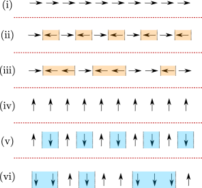
  Figure 1: Schematic representation of the six families of equilibrium points (i)-(vi) discussed in the main text in terms of the angle $x_{i}$.

• The two configurations with $\{x_{i}=\pi/2,\forall i\}$ or $\{x_{i}=-\pi/2,\forall i\}$ (Fig. 1 (iv)) which are saddle points (see Appendix A) with energy $E_{s2}=3N$ (shifted by $2N$).

• The configurations with alternating $\pi/2$ and $-\pi/2$, $\{x_{i}=\pm(-1)^{i}\pi/2,\forall i\}$ (Fig. 1 (v)) which represent saddle points (see Appendix A) with energy $E_{s3}=N$ (shifted by $2N$).

• Configurations of alternating $2b$ blocks of an arbitrary number of dipoles $n_{i}$ ($i=1,2,\ldots,2b$) where within each block $i$ all $n_{i}$ dipoles are either oriented as $x_{k}=\pi/2$ or $x_{k}=-\pi/2$. Following the same discussion as in the equilibrium configuration (iii), the potential energy of this configuration is $E_{s2}=3N$ [case (iv)] minus the potential energy excess of all pairs of dipoles left and right to the interfaces of two neighboring blocks with opposite up and down aligned dipoles, such that the total energy is $E_{s4}=3N-4b$ (shifted by $2N$). An example of this configuration is shown in Fig. 1 (vi) where, taking into account the PBC, there are six blocks of dipoles with alternating up and down orientation resulting in a total energy $E_{s4}=18$.

The above six families of critical points (Fig. 1) allow one to get a glimpse of the high complexity of the landscape of the $N$-dimensional potential energy surface $V$ [see Eq. (11)]. The discussed energy hierarchy of these families should be reflected in the dynamics of the dipole chain. In particular, we expect a linear dynamics for small excitations around the potential minimum $E_{m}=0$ and a quite regular behavior for total excitation energies $E$ below the energy of the lowest saddle point, i.e. for $E<\min\left(E_{s1}\right)=8$. However, for $E>8$, and due to the larger accessible phase space regions which involve also different equilibria, we expect to encounter a nonlinear behavior. It is worth noting that for values of $b$ close to one, the energy $E_{s1}=8b$ of the corresponding saddle points is much smaller than the maximum energy $E_{M}=4N$ of the potential $V$. Hence, one should expect nonlinear behavior even for small excitation energies $E\gtrsim\min\left(E_{s1}\right)=8$.

In the following, we present results for the dynamics of the dipole chain for different excitation energies, spanning the three aforementioned regions with qualitatively different dynamical behavior, i.e. the linear ($E\ll 8$), the regular ($E\lesssim 8$) and the irregular ($E\gtrsim 8$) regime.

III The linear behavior

The equations of motion of the Hamiltonian (10) can be written as:

$$\ddot{x}_{i}=-(\cos x_{i}\sin x_{i+1}+2\sin x_{i}\cos x_{i+1}+\cos x_{i}\sin x_{i-1}+2\sin x_{i}\cos x_{i-1})$$ ((13))

For low-energy excitations, e.g., small oscillations around the head-tail equilibrium configuration $\{x_{i}=0,\forall i\}$ or $\{x_{i}=\pi,\forall i\}$ of minimum energy $E_{m}$, the linear approximation of the equations of motion (13) yields

$$\ddot{x}_{n}=-(x_{n-1}+4x_{n}+x_{n+1}),\quad n=1,...,N.$$ ((14))

As it is well-known, the system of linear differential equations (14) can be solved in terms of $N$ normal modes $(Q_{k},P_{k})$ cross1955 ,

$$Q_{k}(t) = \frac{1}{\sqrt{N}}\sum_{n=1}^{N}x_{n}(t)\exp\left(i\frac{2\pi kn}{N}\right),\quad k=1,...,N$$

$$P_{k}(t) = \frac{1}{\sqrt{N}}\sum_{n=1}^{N}p_{n}(t)\exp\left(i\frac{2\pi kn}{N}\right),\quad k=1,...,N,$$

where $p_{n}(t)=\dot{x}_{n}(t)$.

In the normal mode variables $(Q_{k},P_{k})$, the Hamiltonian $H_{0}$ associated to the linear system (14) reads

$$H_{0}=\sum_{k=1}^{N}{\cal E}_{k}=E_{0},\qquad{\cal E}_{k}=\frac{1}{2}\left(|P_{k}|^{2}+\omega_{k}^{2}\ |Q_{k}|^{2}\right),\quad k=1,...,N$$ ((16))

where $\omega_{k}$ and ${\cal E}_{k}$ are the frequency and the (harmonic) energy of each normal mode, respectively. The sum of the energies of all normal modes $\{{\cal E}_{k}\}$ yields the total harmonic energy $E_{0}$, corresponding to the Hamiltonian $H_{0}$ of the linearized system (14). The frequency $\omega_{k}$ relates to the wave number $k$ through the dispersion relation

$$\omega_{k}=\sqrt{4+2\cos q},\quad q=\frac{2\pi k}{N}$$ ((17))

derived from Eqs. (14)-III. The above expression (Eq. (17)) has already been deduced in e.g. the study of molecular chains Ratner1 and has the form depicted in Fig. 2(red solid line). As expected, the frequency $\omega_{k}$ is 2$\pi$-periodic with $q$ and it enjoys a reflection symmetry with respect to $q=0$ and $\pi$. As we can observe in Fig. 2(solid red line), the linear spectrum is optic-like with the frequency $\omega_{k}$ possessing an upper bound (maximum) $\omega_{k}=\sqrt{6}$ for $q\rightarrow 0$ (long-wavelength limit) and a lower bound (minimum) $\omega_{k}=\sqrt{2}$ for $q=\pi$ (short wavelength limit).

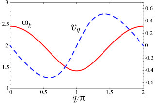
Figure 2: Dispersion relation $\omega_{k}$ (red solid curve) and group velocity $v_{q}$ (blue shaded curve) as a function of $q/\pi$ with $q=2\pi k/N$ being the wave number.

From the dispersion relation (17), the group velocity $v_{q}$ of the normal modes can be derived

$$v_{q}=\frac{d\omega_{k}}{dq}=-\frac{\sin q}{\omega_{k}}.$$ ((18))

As shown in Fig. 2 (blue shaded line), $v_{q}$ vanishes when $\omega_{k}$ reaches its maximum or minimum value, indicating that the normal modes with the longest and the shortest wavelengths are non–propagating modes. In contrast, for $q/\pi=\arccos(-2+\sqrt{3})/\pi\approx 0.59$ and $q/\pi=1+\arccos(2-\sqrt{3})/\pi\approx 1.41$ the group velocity reaches its maximum amplitude $|v_{q}|\approx 0.52$, rendering the corresponding normal modes the fastest propagating ones in the system.

In the current study we are interested in the time propagation of single dipole excitations through the dipole chain for different values of the excitation energy. More specifically, starting from the head-tail configuration (Fig. 1(i)) of minimal energy $E_{m}=0$, we excite at $t=0$ a single dipole, supplying it with an excess energy $\Delta K$. In all our calculations we use a chain of 200 dipoles with PBC, a fact that allows us to excite a specific dipole (here the $100$th) without loss of generality. The initial conditions $(x_{i}(0),p_{i}(0))$ of our system at $t=0$ are given therefore by

$$x_{i}(0) = p_{i}(0)=0,\qquad\mbox{for}\quad i\neq 100,$$

$$\Delta K = \frac{p_{100}(0)^{2}}{2}+4[1-\cos x_{100}(0)].$$ ((19))

Using these initial conditions, we investigate the time propagation of the excitation by integrating numerically the equations of motion (13) for the dipole chain. In order to achieve a high accuracy, we integrate Eqs. (13) using an explicit Dormant–Prince Runge–Kutta algorithm of eighth order with step size control and dense output hairer . The results of these integrations are subsequently compared to those extracted by a symplectic and symmetric Gauss method of six stages hairer2 . Up to the same prescribed error tolerances, in all cases the numerical results obtained with both methods are the same.

During the integration we record at each time step, besides the phase space variables $x_{i}(t)$ and $p_{i}(t)$ of each dipole, also the harmonic energy contribution ${\cal E}_{k}(t)=\frac{1}{2}\left(|P_{k}(t)|^{2}+\omega_{k}^{2}\ |Q_{k}(t)|^{2}\right)$ of each Fourier mode $(Q_{k}(t),P_{k}(t))$ resulting from the Fourier transform (Eq. III) of the numerically extracted $\{x_{i}(t),p_{i}(t)\}$. We emphasize here that all these quantities are recorded for the exact equations of motion (Eq. (13)) of our system and not for their linearized form (Eq. (14)) discussed above.

As we have briefly mentioned in the previous section, for very low values of the excitation energy $\Delta K\ll 8$ (much lower than the energy of the first saddle point) we expect a linear behavior of the dipole chain, with the Eqs. (14) describing appropriately the small oscillations of the dipoles around the head-tail equilibrium configuration. In this linear regime, the harmonic energy ${\cal E}_{k}(t)$ stored in each Fourier mode $(Q_{k}(t),P_{k}(t))$ remains almost constant in time, since the Fourier modes are the approximate (uncoupled) normal modes of the system, and therefore the total excitation energy $\Delta K$ is roughly equal to the total harmonic energy $E_{0}(t)=\sum_{k=1}^{N}{\cal E}_{k}(t)$ distributed among the $N$ Fourier modes of the system [see Eq. (16)].

For larger excitation energies $\Delta K$ the behavior of the system is expected to be in general nonlinear, involving a transfer of energy between the different Fourier modes $(Q_{k}(t),P_{k}(t))$ due to their coupling. The higher the degree of such a nonlinear mode-coupling, the higher we expect to be the deviation of $\Delta K$ (the total energy of our system, involving all the couplings between the modes) from the total harmonic energy contribution $E_{0}(t)$ resulting from the modes $(Q_{k}(t),P_{k}(t))$ which are assumed to be uncoupled. Therefore, we can use this deviation between $\Delta K$ and $E_{0}(t)$ as an indicator of the degree of nonlinearity in the system.

In particular, we define the function $C_{1}(\Delta K)$

$$C_{1}(\Delta K)=\frac{<{E_{0}}>}{\Delta K},\quad\left<E_{0}\right>=\frac{1}{t_{f}}\int_{0}^{t_{f}}E_{0}(t)\ dt,$$ ((20))

where $\left<E_{0}\right>$ is the time average of the total harmonic energy $E_{0}(t)$ of the Fourier modes $\{Q_{k}(t),P_{k}(t)\}$ up to a (large) final time $t_{f}$. According to our above discussion $C_{1}(\Delta K)=1$ for a linear system, where the Fourier modes, coinciding with its normal modes, are uncoupled. The closer the function $C_{1}(\Delta K)$ is to $1$, the closer the exact dynamics of the system is expected to be to linear.

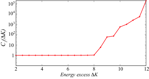
Figure 3: Dependence of $C_{1}(\Delta K)$ [see Eq. (20)] on the excitation energy $\Delta K$ for a single initially excited dipole (Eq. III). Each point of the curve corresponds to the average over an ensemble of 40 simulations with the same initial excess energy but for different initial conditions. Note that a logarithmic scale scale is used for $C_{1}(\Delta K)$.

We present in Fig. 3 the behavior of $C_{1}(\Delta K)$ for excess energies $\Delta K\in[2,12]$. Apart from the time average in the definition of $C_{1}(\Delta K)$ (Eq. (20)), we have also performed for each point of Fig. 3 an average over $40$ different sets of initial conditions (different choices of $x_{100}(0)$ and $p_{100}(0)$, all corresponding to the same excess energy $\Delta K$, see Eqs.  III). We observe that for $\Delta K<8$ the dynamics of the system is only weakly nonlinear, since the average of the total harmonic energy contribution $\left<E_{0}\right>$ of the Fourier modes is a good approximation to the total energy $\Delta K$ of the system ($C_{1}(\Delta K)\approx 1$). In this region we expect that the linear normal modes couple only weakly, leading to minor energy transfer between different modes, but keeping the corresponding harmonic total energy $E_{0}(t)$ approximately constant, equal to $\Delta K$.

In contrast, for excess energies $\Delta K>8$ the value of $C_{1}(\Delta K)$ increases rapidly, with the average total harmonic energy $\left<E_{0}\right>$ of the Fourier modes obtaining much larger values than the total excitation energy $\Delta K$, a fact that indicates a highly nonlinear behavior. Although the value $\Delta K=8$ cannot be considered as a precise threshold between the regimes of a weakly and a highly nonlinear behavior, this value can be perceived as an upper bound, above which the system reacts to localized energy excitations in a highly nonlinear way. It is worth noting that this upper bound ($\Delta K\approx 8$) coincides with the energy $E_{s1}=8$ of the lowest saddle point consisting of two blocks of dipoles with opposite polarization. After overcoming the energetic barrier of the first saddle point, the available phase space of the system increases dramatically, offering possibilities for various dynamical behaviors. Interestingly, we see that the total harmonic energy contribution $E_{0}$ of the Fourier modes is always larger than the total energy $E\equiv\Delta K$ of the system. In other words, the contribution of the coupling between the Fourier modes to the energy, representing the nonlinear interaction, is negative, e.g., it is attractive.

This observation can be justified by the $4$th-order expansion of the total potential $V$ (Eq. (11)) around the equilibrium position $\{x_{i}=0,\forall i\}$. Such an expansion yields

$$V\approx V_{1}=\sum_{i=1}^{N}\left(x_{i}^{2}+x_{i+1}^{2}+x_{i}x_{i+1}\right)-\sum_{i=1}^{N}\left(\frac{(x_{i}^{2}+x_{i+1}^{2})(x_{i}+x_{i+1})^{2}}{12}+\frac{x_{i}^{2}\ x_{i+1}^{2}}{3}\right),$$ ((21))

where the negative energy contribution of the nonlinear terms to the total potential energy is clearly observed. The potential $V_{1}$ resembles the Fermi-Pasta-Ulam ${\beta}$-model (FPU-${\beta}$) with a potential of the form $V_{FPU-\beta}=\sum_{i=1}^{N}\left[\frac{1}{2}{\left(x_{i}-x_{i+1}\right)^{2}}+\frac{\beta}{4}\left(x_{i}-x_{i+1}\right)^{4}\right]$, since both contain only quartic nonlinear terms. However, in our model, in contrast to the FPU models, the degree of nonlinearity is fixed and cannot be controlled by varying the system parameters (such as $\beta$). Besides, while the linear spectrum of our problem is optic-like (Fig. 2), the FPU models display an acoustic-like linear spectrum A867 ; A837 with no frequency gap for long wavelengths $q\rightarrow 0$.

IV The Weakly Nonlinear Regime

In this section we present in detail the response of the dipole chain to single local perturbations in the weakly nonlinear regime of small excitation energies ($\Delta K<8$). Following a similar scheme as in Sec. III, given a chain of 200 dipoles with PBC in the head-tail configuration of minimal energy $E_{m}=0$, we locally excite at $t=0$ the 100th dipole of the chain by supplying it with an excess of kinetic energy $\Delta K$. Thus, the initial conditions $(x_{i}(0),p_{i}(0))$ of our system at $t=0$ read

$$x_{i}(0) = p_{i}(0)=0,\qquad\mbox{for}\quad i\neq 100,$$

$$x_{100}(0) = 0,\quad p_{100}(0)=\sqrt{2\Delta K}.$$ ((22))

In order to study the propagation of this initially localized excitation along the dipole chain we calculate numerically the time evolution of the local energies $E_{k}(t)$

$$E_{k}(t) = \frac{p_{k}(t)^{2}}{2}+\frac{1}{2}\bigg{[}\sin x_{k}(t)\sin x_{k+1}(t)-2\cos x_{k}(t)\cos x_{k+1}(t)+$$

$$\sin x_{k}(t)\sin x_{k-1}(t)-2\cos x_{k}(t)\cos x_{k-1}(t)\bigg{]},$$

which indicate the amount of energy stored in each dipole in relation to its nearest neighbours.

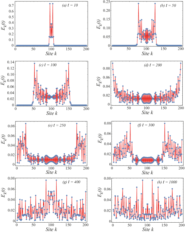
Figure 4: Spatial (site) distribution of the local energies $E_{k}(t)$ for different time instants. The number of dipoles in the chain is $N=$200 and the initial kinetic energy excess provided to the central dipole at site 100 is $\Delta K=4$.

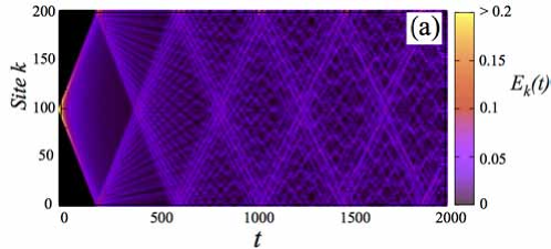
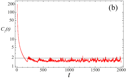
Figure 5: a) Time evolution of the local energy $E_{k}(t)$ of the dipoles (depicted by color). The number of dipoles in the chain is $N=$200 and the initial kinetic energy excess provided to the central dipole at site 100 is $\Delta K=4$. b) Time evolution of the inverse participation ratio $C_{2}(t)$ (Eq. (24)) for $N=$200 and $\Delta K=4$. Note that a logarithmic scale is used for $C_{2}(t)$.

The local energy profiles for $\Delta K=4$ at different time instants shown in Fig. 4 provide a glimpse of the different steps of the excitation propagation. Shortly after the excitation, most of the excess energy is transfered to the nearest neighbors of the initially excited dipole ($100$th), which become the main energy carriers initiating the energy spreading along the chain. Indeed, at short times $t=10,50$ and $100$ [see Figs.4(a)-(c)], the excitation transfer is clearly induced by two (symmetric) energy fronts that propagate along the chain. At $t\approx 200$, the energy excitation reaches the ends of the chain [see Fig.4(d)] having transfered an amount of energy to every dipole in the chain, causing their oscillations. This yields a propagation velocity $v_{p}\approx 0.5$, close to the maximum value of the group velocity $|v_{q}|\approx 0.52$ found for the linear case (see Eq. (18)).

Due to the PBC of the system for $t\gtrsim 200$ the excitation continues its propagation from the outer dipoles (at sites 1, 200) to the inner ones (located at sites around 100), i.e. the direction of propagation is reversed such that for $t\approx 400$ the excitation reaches again the central dipoles of the chain [see Figs.4(e)-(g) corresponding to $t=250,300$ and $400$]. As the chain is progressively excited, the sharp intensity peaks of the propagation fronts observed at short times (Fig.4(a)) decays significantly (Figs.4(e)), indicating that the system tends to thermalize, reaching for long times energy equipartition [see Fig. 4(h) for $t=1000$].

According to the above discussion, a global picture of the time evolution of the local energy $E_{k}(t)$ is given in terms of a color map in Fig. 5 (a). After the $100$th dipole is excited with an excess energy $\Delta K=4$, the excitation energy is gradually distributed along the chain by means of the two aforementioned symmetric energy fronts. As the system approaches the energy equipartition state, the energy fronts are distorted and their intensity decreases.

To quantify the localization of the energy along the chain, we use the following function, usually termed as the inverse participation ratio A851

$$C_{2}(t)=N\frac{\sum_{k=1}^{N}E_{k}(t)^{2}}{\Delta K^{2}},$$ ((24))

with $E_{k}$ being the local energies given by Eq. IV. When the excitation is maximally localized, i.e. the total excitation energy energy $\Delta K$ of the system is carried by a single dipole, the value of $C_{2}$ is $N$, while if there is complete equipartition ($E_{k}\approx\Delta K/N~{}\forall k$) $C_{2}=1$. The time evolution of $C_{2}$ is shown in Fig. 5 (b). Starting from a fully localized excitation ($C_{2}(0)=200$) the excitation propagation quickly leads to a regime where the excitation energy is almost equally partitioned among all the dipoles ($C_{2}\lesssim 2$).

V The highly NonLinear Regime

Following the same scheme as in Sec. IV, we excite at $t=0$ the 100th dipole from the head-tail ground state of a 200-dipole chain, supplying it with a kinetic energy excess $\Delta K>8$.

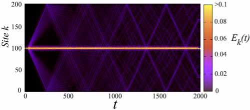
Figure 6: Time evolution of the local energy $E_{k}(t)$ of the dipoles (depicted by color). The number of dipoles in the chain is $N=$200 and the initial kinetic energy excess given to the central dipole 100 is $\Delta K=12$.

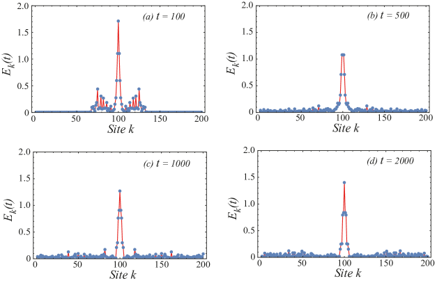
Figure 7: Spatial (site) distribution of the local energies $E_{k}(t)$ for different time instants. The number of dipoles in the chain is $N=$200 and the initial kinetic energy excess given to the central dipole at site 100 is $\Delta K=12$.

A typical propagation scheme in this highly nonlinear regime is the one obtained for an excess energy $\Delta K=12$. For this value the time evolution of the spatial distribution of the local energies $E_{k}(t),~{}k=1,2,\ldots 200$ is depicted in Fig. 6. We observe a robust excitation around the $100$th dipole, indicating that the system does not reach energy equipartition up to long times. Indeed, the initially excited dipole $100$ shares predominantly energy with a few of its neighbors so that a significant part of the excess energy remains localized around it.

This fact is emphasized in Fig. 7 where the local energy profiles for $t=$100, 500, 1000 and 2000 are depicted. At short times (see Fig. 7(a) for $t=$100) a small propagation front emerges whose energy after some time is distributed among all the dipoles of the chain (see Fig. 7(b) for $t=$500). However, the excitation energy of the few central dipoles (close to the initially excited one) remains much larger than that of the other outer dipoles, creating overall a highly localized profile which persists in time (see Fig. 7(c)-(d)).

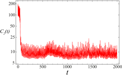
Figure 8: Time evolution of the inverse participation ratio $C_{2}(t)$ for a kinetic energy excess $\Delta K=12$.

As in the previous section, the degree of localization of this local excitation with an energy excess $\Delta K=12$ can be quantified by means of the inverse participation ratio $C_{2}$ (Eq. (24)). In its time evolution, shown in Fig. 8, we observe a rapid decrease followed by asymptotic high-amplitude oscillations around $C_{2}\approx 10$. This asymptotic value of $C_{2}$ is an order of magnitude larger than the corresponding value of $C_{2}$ in the weakly nonlinear regime (see Fig. 5 (b)), which points to the much stronger localization of the excitation. This high degree of localization suggests the existence of a strong nonlinearity since, for the linear case the dispersion of the excitation energy along the complete chain dominates the dynamics, leading to an approximately equipartition regime in terms of local energies $E_{k}$.

Even more, it turns out that the localization of the excitation energy in Figs. 6-7 can be linked to discrete breather solutions of the nonlinear equations of motion of our system (Eq. (13)). Briefly speaking, a discrete breather is a spatially localized exact periodic solution of the nonlinear equations of motion of a given discrete lattice (for more details, we refer the reader to A867 ; A868 ). The non-resonant condition between the frequency $\Omega$ of a breather solution and the dispersion relation $\omega_{k}$ prevents the existence of breathers with a frequency in the linear spectrum, such that the breather frequency $\Omega$ should always lie outside the linear spectrum $\omega_{k}$. In our system, for $\Delta K=12$, we have seen (Fig. 7) that a major part of the excitation energy $\Delta K$ stored initially on the $100$th dipole remains localized in the few dipoles surrounding it up to long times. Moreover, when the time evolution of the angles $x_{99}(t)$ and $x_{100}(t)$ of the dipoles 99 and 100 respectively are examined (see Fig.9), we find that their motion is in both cases fairly periodic (oscillatory) with a period of $\tau\approx 6.7$. The periodicity of these oscillations is justified by Fig. 10, where the Fourier spectra of $x_{99}(t)$ and $x_{100}(t)$ are depicted. Indeed, we observe that these spectra exhibit a strong peak at a frequency $f\approx 0.15$ (with its symmetric counterpart at $f\approx 0.85$), reflecting the fact that the corresponding signals can be approximated as oscillations with a single frequency $\Omega=2\pi f\approx 2\pi\times 0.15\approx 0.94$, corresponding to a period of $\tau\approx 6.67$. Since this oscillation frequency, $\Omega\approx 0.94$, is outside (more precisely below) the linear spectrum depicted in Fig. 2 (red line), we have strong evidence that the localized excitation of the dipole chain observed in Figs. 6-7 during its time evolution corresponds to a discrete breather.

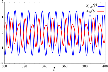
Figure 9: Time evolution of the angles $x_{99}(t)$ and $x_{100}(t)$ of the dipoles 99 and 100 in the interval $300\leq t\leq 400$. Excess energy is $\Delta K=12$.

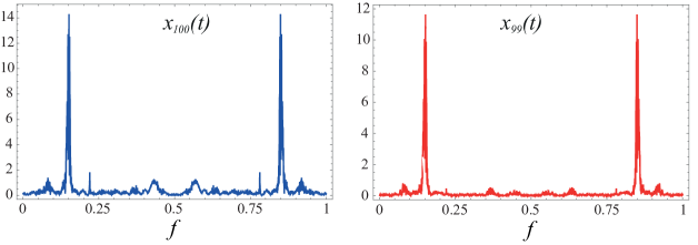
Figure 10: Fourier spectra of $x_{99}(t)$ and $x_{100}(t)$ of the dipoles 99 and 100. The excess energy $\Delta K=12$ is provided to the 100th dipole.

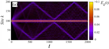
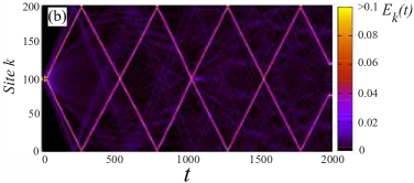
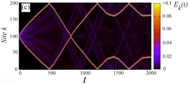
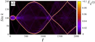
Figure 11: Time evolution of the local energy $E_{k}(t)$ of the dipoles (depicted by color) for four values of the excess energy (a) $\Delta K$=10.776, (b) $\Delta K$=11.128, (c) $\Delta K$=10.2 and (d) $\Delta K$=11.12.

Besides the typical discrete breather pattern of energy localization shown in Fig. 6, the dipole chain exhibits additional propagation schemes, depending on the value of the initial excitation energy $\Delta K$, all of them involving a high degree of energy localization. The time evolutions for the local energies $E_{k}(t)$ for four cases $\Delta K$ = 10.776, 11.128, 10.2 and 11.12, corresponding to different propagation patterns, are shown in Figs. 11(a)-(d). The main difference between these is the behavior of the principal energy carriers, i.e. the dynamics of those sites that carry the largest amount of excitation energy. For $\Delta K$ = 10.776 and 11.128 [Fig. 11(a)-(b)], the energy of the system is highly localized in two energy carriers that follow trajectories of a regular periodic character. In contrast, for $\Delta K$ = 10.2 and 11.12 [Fig. 11(c)-(d)] the principal energy carriers follow rather complex trajectories which, given their strong localization and complexity, could be linked to the so-called chaotic breathers A851 . Contrary to the concept of a discrete breather as a localized excitation which is a solution of the nonlinear equations of motion of the lattice, a chaotic breather is an excitation of chaotic nature that may appear as a response to initial local excitations of the lattice, a situation that, as it will be argued below, bears strong similarities to the one described here regarding the propagation of a localized excitation in our dipole chain in the highly nonlinear regime ($\Delta K\gtrsim 8$).

Apart from the different patterns of energy propagation observed in Fig. 11 for the different values of $\Delta K$, it turns out that also the configurations $\{x_{k}\}$ evolve differently in time. We illustrate this fact in Fig. 12 where the time evolution of $\cos(x_{k}(t))$ is shown for the same excitation energies, $\Delta K=$10.776, 11.128, 10.2 and 11.12, as those considered in Fig. 11. For $\Delta K=10.776$ and $11.128$ (see Figs. 12(a)-(b)) we observe the expected behavior: except for the energy carrying rotors (ECRs), which exhibit fast long-amplitude oscillations (fast changing $x_{k}$) while propagating along the chain leading to the corresponding traces in Figs. 12(a)-(b), all the remaining dipoles are mainly polarized in the same direction $\{x_{k}=0\}$ ($\cos(x_{k})=1$) as in the ground state configuration.

 

 

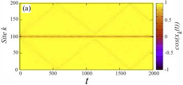
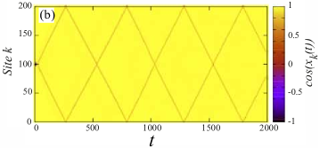
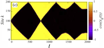
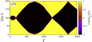
Figure 12: The time evolution of $\cos(x_{k})$ (depicted by color) for different values of the excess energy $\Delta K$: (a) $\Delta K$=10.776, (b)$\Delta K$=11.128, (c)$\Delta K$=10.2 and (d) $\Delta K$=11.12. as in Fig.11.

In contrast, for $\Delta K=10.2$ and $11.12$ (Fig. 12(c)-(d)) the situation is dramatically different. Instead of a single polarized region ($\cos(x_{k})=1$), like the yellow background in Figs. 12(a)-(b), two regions of opposite polarization ($\cos(x_{k})=1$ and $\cos(x_{l})=-1$ ) emerge during the time evolution. These regimes of locked phases ($\{x_{k}=0\}$ and $\{x_{l}=\pi\}$ respectively) corresponding to domains of opposite polarization appear spontaneously and they are dynamically separated by two propagating domain walls provided by the two fast rotating ECRs (compare Figs. 12 (c),(d) with Figs. 11 (c),(d). In particular, in the course of the dynamics, the dipoles lying between the two ECRs spontaneously flip, forming a domain of opposite polarization ( $\cos(x_{l})=-1$, black region in Figs. 12 (c),(d)) compared to that of the ground state (yellow region in Figs. 12 (c),(d)).

Although the origin of this spontaneous phase locking is not entirely clear, it can be related to the existence of the lower saddle point equilibria of energy $E_{s1}=8<\Delta K$, ($b=1$, Sec.II.A. (iii) ). This assumption relies on the resemblance of the topology between the phase locked states and the highly degenerate saddle point equilibrium configurations consisting of two blocks: one with a given number $n$ of dipoles with $x_{l}=\pi$ and another with the remaining $N-n$ dipoles polarized along $x_{k}=0$. As mentioned in Sec. II, all such saddle points, consisting of two domains of opposite polarization are highly degenerate, since their total potential energy $E_{s1}=8$ depends only on the number of domain walls (here two) and not on the number of dipoles on each domain ($n$ and $N-n$ respectively). With an excitation energy $\Delta K=12>E_{s1}$ a spontaneous dynamical transition from the fully polarized ground state to the first saddle point is energetically possible and therefore can occur for certain initial conditions (Figs. 12(c)-(d)). During the time evolution of such a state the domain walls, identified with the ECRs, shift (Figs. 12(c)-(d)), following the complex trajectories shown in Figs. 11(c)-(d), a process that due to the aforementioned degeneracy of the first saddle point does not cost any energy.

It is worth noticing that phase locked states with more than two domains (more than two domain walls) never appear in our simulations considering an excitation energy $\Delta K\in[4,12]$, since already the energy of the second saddle point, $E_{s1}=16$, consisting of four domains (four domain walls), is inaccessible. It should be observed, however, for $\Delta K>16$.

A closer look at Fig. 11 and Fig.12, particularly a comparison between Fig. 11(b) and Fig. 11(d) (also between Figs. 12(b) and Figs. 12(d)), leads to the conclusion that even a tiny change of the excitation energy $\Delta K$ (here only by $0.07\%$) can lead to a completely different propagation and configuration pattern. We have checked that this is the case also when a infinitesimal perturbation is added to the initial values of the phase space variables ($x_{i}(0),p_{i}(0)$). This strong sensitivity to the initial conditions is the hallmark of the chaotic nature of our system in the region of excitation energies $\Delta K>8$.

As a measure of this sensitivity to the initial conditions in the dipole chain (i.e. its degree of chaoticity), we use the method of the Orthogonal Fast Lyapunov Indicators (OFLI). In a nutshell, given an m-dimensional flow defined by

$$\frac{d{\bf r}}{dt}={\bf f}({\bf r},t),$$ ((25))

we examine the time evolution of the variational vector $\delta{\bf r}(t)$ given by the (first) variational equations

$$\frac{d\delta{\bf r}}{dt}=\frac{\partial{\bf f}({\bf r},t)}{\partial{\bf r}}\delta{\bf r}.$$ ((26))

For given initial conditions ${\bf r}(0)$ and $\delta{\bf r}(0)$, the numerical integration of the systems of differential equations (25) and (26) up to a given final time $t_{f}$ allows the definition of the OFLI as follows ofli2 ; ofli22 ; A709

$$\mbox{OFLI}({\bf r}(0),\delta{\bf r}(0),t_{f})=\sup_{0\leq t\leq t_{f}}\log||\delta{\bf r}(t)^{\bot}||,$$ ((27))

where $\bot$ indicates the orthogonal component to the flow of the variational vector $\delta{\bf r}$. The main advantage of the OFLI is that it provides computationally cheap information about the degree of regularity/chaoticity of a given orbit. In particular, $\delta{\bf r}(t)^{\bot}$ increases linearly with time for regular resonant orbits and exponentially for chaotic ones  ofli2 ; ofli22 ; A709 , attaining therefore for long times $t_{f}$ much larger values for chaotic orbits than the ones for regular orbits. For near-integrable Hamiltonian systems, a rigorous proof of this behavior can be found in A709 . We note that with the formulation (27), there is a dependence of the value of the OFLI on the initial conditions of the variational vector $\delta{\bf r}(0)$. In order to get rid of this dependence we follow the steps found in barrio ; barrio1 , incorporating also the second order variational equations in the computation of the indicator. For our dipole chain, we have calculated, as a function of the energy excess $\Delta K$, the OFLI for trajectories as those examined so far, featuring initially a single dipole excitation with initial conditions ${\bf r}(0)=\{x_{k}(0)=0~{}\forall k,p_{100}(0)=\sqrt{2\Delta K},p_{k}(0)=0~{}\forall k\neq 100\}$. In our calculations, we stop the computation of the OFLI either when it reaches the cutoff value 9, marking a chaotic trajectory, or when the computation time exceeds our final time $t_{f}=5000$, selected empirically according to many numerical simulations.

As an example, we present in Fig. 13(a) the time evolution of the OFLI for two qualitatively different orbits, belonging to the weakly (initial kinetic energy excess $\Delta K=4$) and to the highly (initial kinetic energy excess $\Delta K=12$) nonlinear regimes, respectively. We observe in Fig. 13(a) that the OFLI for the $\Delta K=4$ trajectory increases very slowly, attaining only small values (less than two up to very long times). In contrast the OFLI for the $\Delta K=12$ trajectory shows a fast increase reaching already at an early stage the cutoff value nine signifying its chaoticity. Note that at our usually selected final simulation time $t_{f}=5000$ the distinction between the two trajectories is clear, allowing for their classification as regular ($\Delta K=4$) and chaotic ($\Delta K=12$) respectively.

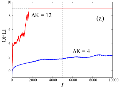
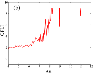
Figure 13: (a) Time evolution of the OFLI for $\Delta K$=4 (blue line) and $\Delta K$=12 (red line). The vertical and horizontal black dashed lines indicate the cutoff value of the OFLI computation and the selected final time $t_{f}=5000$ in our simulations, respectively. (b) The OFLI for a dipole chain with a single excited dipole as a function of the excitation energy $\Delta K$. Note that there is a cutoff value of the OFLI for the value 9.

Our results for the behavior of the OFLI as a function of the excess energy $\Delta K$ are shown in Fig. 13(b). In the regime $\Delta K\lesssim 6$, the value of the OFLI is below three, indicating the regular behavior of the system in accordance to Fig. 3 and the above discussion. For $6\lesssim\Delta K\lesssim 8$, the value of the OFLI increases for increasing energy, such that for $\Delta K\gtrsim 8.5$ it becomes larger than the cut-off value nine characterizing the chaotic orbits. Moreover, the extracted chaoticity of the dipole chain for excitations with energy $\Delta K\gtrsim 8$ provides further evidence for the link of the traveling energy localization patterns shown in Fig. 11 (c),(d) and the striking phase locking states associated to them (Fig. 12 (c),(d)) to chaotic breathers A851 , mentioned above.

As a final remark, it is worth noticing that, in general, the effectiveness of the fast Lyapunov indicators in providing a first indication of the degree of chaoticity of an orbit with a relatively low computational cost has been successfully proven in dynamical systems with few degrees of freedom. Indeed, a global vision of the phase space structure of several Hamiltonian systems with two or three degrees of freedom was obtained by the computation of two-dimensional OFLI maps barrio ; barrio1 ; PRE2014 . However, a detailed investigation of the phase space and the chaotic dynamics of multidimensional systems as our dipole chain requires the use of more sophisticated tools based on the computation of Lyapunov exponents osedelec ; lichtemberg ; skokos as deviation vector distributions A908 and Lyapunov Weighted Dynamics A911 ; A910 . Although very interesting, these investigations go beyond the goal of the present study and will be addressed in a future work.

VI Conclusions

We have explored the energy transfer mechanisms in a classical dipole chain, modeled as an array of $N$ rigid dipoles with their positions fixed in space, interacting with their nearest neighbors and restricted to rotate in a common plane. This leads to a Hamiltonian system of $N$ degrees of freedom describing the rotational dynamics of the dipole chain. The equilibrium points of the equations of motion have been identified and analyzed. It turns out that these can be classified in several families according to their stability, pointing to the high complexity of the potential energy surface of the chain of dipoles. A linearization of the equations of motion around the GS configuration has lead to the harmonic approximation of the dipole chain Hamiltonian in terms of normal modes, a fact that has allowed us to extract information about the linear spectrum of the system.

The main focus of this work has been the study of the energy transfer of a localized excitation in the dipole chain for a varying excitation energy. Two regimes with qualitatively different features have been identified. In the first regime of low energy excitations the system exhibits a weakly nonlinear behavior with the initially localized excitation spreading in the dipole chain, leading for large times to energy equipartition among the dipoles. The second regime of higher energy excitations is characterized by a strong nonlinearity causing energy localization in the form of discrete or chaotic breathers. In some cases the formed chaotic breathers attain the character of domain walls, separating domains of dipoles with different polarization. This spontaneous phase locking of the dipole chain can be linked to the properties of the interaction potential and in particular to its lowest energy saddle point.

It turns out that in the highly nonlinear regime the dipole chain is very sensitive to the initial conditions, indicating its chaotic nature. To quantify the degree of chaoticity in the system for different values of the excitation energy we have calculated the Orthogonal Fast Lyapunov Indicator which confirms the above discussed picture. For excitation energies below a certain approximate threshold the dynamics is regular whereas above it is highly nonlinear and chaotic. Interestingly enough this threshold energy has a value close to the energy difference between the first saddle and the minimum of the interaction potential.

Suitable experimental realizations of our model could be provided by polar diatomic molecules trapped in a 1D optical lattice A753 , colloidal polar particles in optical tweezers colloid_ref or by rotating polar molecules in Helium nanodroplets helium_nano . Further theoretical studies could be devoted to the investigation of the effect of an external homogeneous or inhomogeneous electric field on the dynamics and the energy transfer of a dipole chain as the one studied here. Finally the exploration of the dynamics of the dipole chain in the full $2N$-dimensional case would also be of interest owing to its even more complex potential landscape.

Appendix A The character of the critical points

The nature of the critical points can be judged by the eigenvalues of their Hessian matrix. Due to the nearest-neighbor interactions considered in this study, the Hessian is almost tridiagonal, with an exception regarding the last element of the first row and first element of the last row which are different from zero due to the imposed PBC. In the following we discuss the character of the six families of critical points of the dipole chain based on their Hessian eigenvalues.

A.1 The minimum $E_{m}$ and the maximum $E_{M}$

The $N\times N$ Hessian matrix of the critical point $\{x_{i}=0,\forall i\}$ or $\{x_{i}=\pi,\forall i\}$ takes the form:

$$H_{min}=\left(\begin{array}[]{ccccccc}4&1&0&0&...&0&1\\ 1&4&1&0&...&0&0\\ 0&1&4&1&...&0&0\\ ...&...&...&...&...&...&...\\ 0&0&0&0&...&4&1\\ 1&0&0&0&...&1&4\end{array}\right).$$ ((28))

If $N$ is large, the last element of the first row and the first element of the last row have a negligible contribution to the eigenspectrum of $H_{min}$. Thus, in terms of its eigenspectrum the Hessian can be approximated by the tridiagonal matrix

$$H_{min}\approx\left(\begin{array}[]{ccccccc}4&1&0&0&...&0&0\\ 1&4&1&0&...&0&0\\ 0&1&4&1&...&0&0\\ ...&...&...&...&...&...&...\\ 0&0&0&0&...&4&1\\ 0&0&0&0&...&1&4\end{array}\right).$$ ((29))

The $N$ eigenvalues of the matrices (28) and (29) are real because $H_{min}$ is symmetric. Moreover, the eigenvalues $\lambda_{k}$ of the tridiagonal matrix (29) are given by A862

$$\lambda_{k}=4+2\cos\frac{k\ \pi}{(N+1)}.$$

These eigenvalues are positive indicating that also the eigenvalues of the exact matrix (28) would be positive and in turn that the corresponding critical point is a minimum.

Returning to the original Hessian matrix (28), the analytic computation of its characteristic equation gives the following polynomial of degree $N$

$${\cal C}_{even}\equiv\lambda^{N}-a_{N-1}\lambda^{N-1}+a_{N-2}\lambda^{N-2}-...-a_{1}\lambda+a_{0}=0,\quad N\equiv\mbox{even},$$

$${\cal C}_{odd}\equiv\lambda^{N}-a_{N-1}\lambda^{N-1}+a_{N-2}\lambda^{N-2}-...+a_{1}\lambda-a_{0}=0,\quad N\equiv\mbox{odd},$$

where $a_{i}>0$. This means that there are $N$ sign changes in the sequence of the coefficients $(1,a_{N-1},a_{N-2},...,a_{1},a_{0})$. The rule of Descartes descartes , says that if $p$ is the number of positive roots of a given polynomial and $s$ is the number of sign changes in the coefficient sequence of this polynomial, then $s=p+2k$, with $k$ a positive integer. By virtue of this theorem, from the $N$ changes of sign in the coefficients $a_{i}$, we conclude that the Hessian (28) has at most $N$ positive eigenvalues. We can apply the Descartes rule also to extract information about the maximum number of negative roots. Indeed, after replacing $\lambda\rightarrow-\lambda$, the coefficients of the odd degree monomials in $\lambda$ in the characteristic polynomials ${\cal C}_{even,odd}$ become negative, resulting in no sign changes in the coefficient sequence. This implies that there are no negative eigenvalues and as a consequence all the $N$ eigenvalues of the exact Hessian (28) are positive.

For the critical point corresponding to the alternating configuration $\{x_{i}=\pi\left[1\pm(-1)^{i}\right]/2,\forall i\}$, the Hessian matrix takes the form:

$$H_{max}=-H_{min}.$$

with approximate eigenvalues

$$\lambda_{k}=-(4+2\cos\frac{k\ \pi}{(N+1)}),$$

which are all negative,indicating that this critical point is a maximum. The analytic computation of the characteristic equation yields

$${\cal C}_{max}=\lambda^{N}+a_{N-1}\lambda^{N-1}+a_{N-2}\lambda^{N-2}+...+a_{1}\lambda+a_{0}=0$$

where $a_{i}<0$. Therefore, there are no sign changes in the sequence of the coefficients $(1,a_{N-1},a_{N-2},...,a_{1},a_{0})$. In this case, the Descartes rule of signs assures that there are no positive roots of the characteristic polynomial. If we replace $\lambda\rightarrow-\lambda$ in ${\cal C}_{max}$, the coefficients of the odd degree monomials in $\lambda$ become negative, a fact that results in $N$ sign changes in the coefficient sequence. Thus the $N$ eigenvalues of $H_{max}$ are negative and the corresponding critical point is a maximum.

A.2 The saddle points $E_{s1}$

For the configurations made of $b$ blocks of $n_{j}$ dipoles with $x_{k}=\pi$ while the remaining dipoles possess $x_{i}=0$, up to our knowledge, there exists no close expression for the eigenvalues of the corresponding almost tridiagonal Hessian matrix. However, from the numerical computation of the characteristic equation for different values of $N$ and for different number of blocks $b$, we have strong indications that these critical points are saddle points of rank $2b$ since, by applying the rule of Descartes, we find that the number of positive and negative eigenvalues are $N-2b$ and $2b$, respectively.

A.3 The saddle points $E_{s2}$

For the two configurations $\{x_{i}=\pi/2,\forall i\}$ or $\{x_{i}=-\pi/2,\forall i\}$, the Hessian matrix takes the form

$$H_{s3}=\left(\begin{array}[]{ccccccc}-2&-2&0&0&...&0&-2\\ -2&-2&-2&0&...&0&0\\ 0&-2&-2&-2&...&0&0\\ ...&...&...&...&...&...&...\\ 0&0&0&0&...&-2&-2\\ -2&0&0&0&...&-2&-2\end{array}\right).$$ ((30))

Following A862 , the approximate eigenvalues for large $N$ are given by the expression

$$\lambda_{k}=-2+4\cos\frac{k\ \pi}{(N+1)}.$$ ((31))

From Eq. (31), we obtain that this critical point is a saddle point with $2(N+1)/3$ hyperbolic directions.

A.4 The saddle points $E_{s3}$

For the configuration with alternating angles $\pi/2$ and $-\pi/2$, $\{x_{i}=\pm(-1)^{i}\pi/2,\forall i\}$, the Hessian matrix takes the form

$$H_{s3}=\left(\begin{array}[]{ccccccc}2&2&0&0&...&0&2\\ 2&2&2&0&...&0&0\\ 0&2&2&2&...&0&0\\ ...&...&...&...&...&...&...\\ 0&0&0&0&...&2&2\\ 2&0&0&0&...&2&2\end{array}\right).$$ ((32))

Following A862 , the approximate eigenvalues for large $N$ are given by the expression

$$\lambda_{k}=2+4\cos\frac{k\ \pi}{(N+1)}.$$ ((33))

From Eq. (33), we see that this critical point is a saddle point with $(N+1)/3$ hyperbolic directions.

A.5 The critical points $E_{s4}$

For the critical points made of all the possible configurations with $x_{i}=\pm\pi/2$, up to our knowledge, there exists no close expression for the approximate eigenvalues of the corresponding almost tridiagonal Hessian matrix. Moreover, from the numerical computation of the characteristic equation for different configurations, we cannot conclude anything about the nature of these critical points, because, depending on the equilibrium configuration, some of the eigenvalues are zero.

References

- (1) E. Fermi, J. Pasta, and S. Ulam, Studies of the Nonlinear Problems, I, Los Alamos Report LA-1940, (1955); reprinted in Nonlinear Wave Motion, ed. A. C. Newell, Lecture Notes in Applied Mathematics, 15 (AMS, Providence, RI, 1974). and also in Many-Body Problems, ed. D. C. Mattis (World Scientific, Singapore, 1993).
- (2) G. P. Berman and F. M. Izrailev, Chaos 15, 015104 (2005).
- (3) T. Dauxois, Physics Today 61, 55 57 (2008).
- (4) N. J. Zabusky, Chaos 15, 015102 (2005).
- (5) J. Ford, Phys. Rep. 213, 271 (1992).
- (6) The Fermi-Pasta-Ulam Problem. A Status Report, G. Gallavotti (Eds), (Springer-Verlag Berlin Heidelberg, 2008).
- (7) A. Mussot, A. Kudlinski, M. Droques, P. Szriftgiser, and N. Akhmediev, Phys. Rev. X 4, 011054 (2014).
- (8) D. Bambusi, A. Carati, A. Maiocchi, and A. Maspero, Some Analytic Results on the FPU Paradox, pag. 235, in Hamiltonian Partial Differential Equations and Applications, Fields Institute Communications , P. Guyenne, D. Nicholls and C. Sulem (Eds) (Springer Science+Business Media, New York 2015).
- (9) T. Penati and S. Flach, Chaos 17, 023102 (2007).
- (10) R. Livi, M. Pettini, S. Ruffo, M. Sparpaglione and A. Vulpini, Phys. Rev. A 31, 1039 (1985).
- (11) L. Casetti, M. Cerruti-Sola, M. Pettini and E. G. D. Cohen, Phys. Rev. E 55, 6566 (1997).
- (12) M. Pettini, L. Casetti, M. Cerruti-Sola, R. Franzosi and E. G. D. Cohen, Chaos 15, 015106 (2005).
- (13) S. Flach, M. V. Ivanchenko and O. I. Kanakov, Phys. Rev. Lett. 95, 064102 (2005).
- (14) S. Flach. Nonlinear Theory and Its Applications, IEICE 3, 1 (2015).
- (15) S. Flach, and A. V. Gorbach, Phys. Rep. 467, 1 (2008).
- (16) T. Cretegny, T. Dauxois, S. Ruffo, and A. Torcini, Physica D 121, 109 (1998).
- (17) A. J. Lichtenberg, and G. Corso. Phys. Rev. E 61, 2472 (2000).
- (18) Photosynthetic Excitons, H. Van Amerongen, L. Valkunas, R. Van Grondelle, (World Scientific, Singapore, 2000).
- (19) G.S. Engel, T. R. Calhoun, E.L. Read, T.K. Ahn, T. Mancal, Y.C. Cheng, R.E. Blankenship, and G. R. Fleming, Nature 446, 782 (2007).
- (20) Y.-C. Cheng and G. R. Fleming, Annu. Rev. Phys. Chem. 60, 241 (2009).
- (21) J.l. Wu, F. Liu, J. Ma, R. J. Silbey, and J. Cao, J. Chem. Phys. 137, 174111 (2012).
- (22) Energy Transfer Dynamics in Biomaterial Systems, I. Burghardt, V. May, D. A. Micha, and E. R. Bittner (Eds.), (Springer-Verlag Berlin Heidelberg 2009).
- (23) S. K. Saikin, A. Eisfeld, S. Valleau and A. Aspuru-Guzik, Nanophotonics 2, 21 (2013).
- (24) D. Melnikau, D. Savateeva, V. Lesnyak, N. Gaponik, Y. Núnez Fernández, M. I. Vasilevskiy, M. F. Costa, K. E. Mochalov, V. Oleinikov and Y. P. Rakovich, Nanoscale 5, 9317 (2013).
- (25) Y. Qiao, F. Polzer, H. Kirmse, E. Steeg, S. Kühn, S. Friede, S. Kirstein, and J. P. Rabe, ACS Nano 9, 1552 (2015).
- (26) A. S. Davydov, Theory of Molecular Excitons, (New York: McGraw-Hill, 1962).
- (27) R. Silbey, Ann. Rev. Phys. Chem. 27, 203 (1976).
- (28) J. D. Wright, Molecular Crystals, (2nd Edition, Cambridge University Press 1994).
- (29) G. S. Kottas, L. I. Clarke, D. Horinek, and J. Michl, Chem. Rev. 105, 1281 (2005).
- (30) Cold Molecules: Theory, Experiments and Applications, R. Krems, B. Friedrich and W. C. Stwalley (Eds.), (CRC Press, Taylor & Francis, 2009)
- (31) M. Weidemüller and C. Zimmermann (Ed.), Cold Atoms and Molecules, (Wiley–VCH, 2009).
- (32) T. Lahaye, C. Menotti, L. Santos, M. Lewenstein and T. Pfau, Rep. Prog. Phys. 72, 126401 (2009).
- (33) B. Zhu, J. Schachenmayer, M. Xu, F. H. Urbina, J. G. Restrepo, M. J. Holland, A. M. Rey, New J. Phys. 17, 083063 (2015).
- (34) T. Sowiński, O. Dutta, P. Hauke, L. Tagliacozzo, M. Lewenstein, Phys. Rev. Lett. 108, 115301 (2012).
- (35) S. W. DeLeeuw, D. Solvaeson, M. A. Ratner and J. Michl, J. Phys. Chem. B 102, 3876 (1998).
- (36) E. Sim, M. A. Ratner and S. W. de Leeuw, J. Phys. Chem. B 103, 8663 (1999).
- (37) J. J. de Jonge, M. A. Ratner, S. W. de Leeuw and R. O. Simonis, J. Phys. Chem. B 108, 2666 (2004).
- (38) R. González-Férez, M. Iñarrea, J. P. Salas and P. Schmelcher, Phys. Rev. E. 95, 012209 (2017).
- (39) L. Chotorlishvili and J. Berakdar. J. Phys. B: At. Mol. Opt. Phys. 40, 3757 (2007).
- (40) E. B. Wilson, J. C Decius and P.C Cross, Molecular Vibrations (Dover, New York, 1955).
- (41) E. Hairer and G. Wanner, Solving Ordinary Differential Equations I. Non Stiff Problems (Springer-Verlag, New York, 1993).
- (42) E. Hairer, C. Lubich and G. Wanner, Geometric Numerical Integration. Structure-Preserving Algorithms for Ordinary Differential Equations (Springer Series in Computational Mathematics 31, Springer, 2006).
- (43) C. Froeschlé and E. Lega, Celes. Mech. Dyn. Astr. 78, 167 (2000).
- (44) M. Fouchard, E. Lega and C. Froeschlé, Celes. Mech. Dyn. Astr. 83, 205 (2002).
- (45) M. Guzzo, E. Lega, C. Froeschl , Physica D 163, 1 (2002).
- (46) R. Barrio, Chaos, Solitons and Fractals 25, 711 (2005).
- (47) R. Barrio, Int. J. Bif. and Chaos 16, 2777 (2006).
- (48) R. González-Férez, M. Iñarrea, J. P. Salas and P. Schmelcher, Phys. Rev. E. 90, 062919 (2014).
- (49) V. I. Osedelec, Trans. Moscow Math. Soc. 19, 197 (1968).
- (50) A. Lichtenberg and M. Lieberman , Regular and Chaotic Dynamics (Springer Science, New York, 1992).
- (51) Skokos C. , The Lyapunov Characteristic Exponents and Their Computation. Dynamics of Small Solar System Bodies and Exoplanets. Lecture Notes in Physics, 790, 63-135. (Springer-Verlag ,Berlin, Heidelberg, 2010).
- (52) Ch. Skokos I. Gkolias and S. Flach, Phys. Rev. Lett. 111, 064101 (2013).
- (53) P. Geiger, C. Dellago, Chem. Phys. 375, 309 (2010).
- (54) T. Laffargue, K.-D. Nguyen Thu Lam, J. Kurchan and J. Tailleur, J. Phys. A: Math. Theor. 46, 254002 (2013).
- (55) M. Mittal, P. P. Lele, E. W. Kaler and E. M. Furst, J. Chem. Phys. 129, 064513 (2008)
- (56) B. Shepperson, A. A. Søndergaard, L. Christiansen, J. Kaczmarczyk, R. E. Zillich, M. Lemeshko and H. Stapelfeldt, Phys. Rev. Lett. 118, 203203 (2017)
- (57) W.-C. Yueh. Applied Mathematics E-Notes 5, 66 (2005).
- (58) J. Stoer and R. Bulirsch, Introduction to Numerical Analysis (Springer-Verlag, New York, 1983).