Long-wavelength phonons in the crystalline and pasta phases of neutron-star crusts

Abstract

We study the long-wavelength excitations of the inner crust of neutron stars, considering three phases: cubic crystal at low densities, rods and plates near the core-crust transition. To describe the phonons, we write an effective Lagrangian density in terms of the coarse-grained phase of the neutron superfluid gap and of the average displacement field of the clusters. The kinetic energy, including the entrainment of the neutron gas by the clusters, is obtained within a superfluid hydrodynamics approach. The potential energy is determined from a model where clusters and neutron gas are considered in phase coexistence, augmented by the elasticity of the lattice due to Coulomb and surface effects. All three phases show strong anisotropy, i.e., angle dependence of the phonon velocities. Consequences for the specific heat at low temperature are discussed.

I Introduction

In the inner crust of neutron stars, neutron-rich nuclei (clusters) coexist with a gas of unbound neutrons and a degenerate electron gas Chamel and Haensel (2008). To minimize the Coulomb energy, the clusters form a periodic lattice. Close to the transition to the neutron-star core, the competition between Coulomb and surface energy leads to the so-called “pasta phases”: while the clusters are assumed to be spherical at low density (crystalline phase), they merge with increasing density to form rods (“spaghetti phase”) and then plates (“lasagne phase”) Ravenhall et al. (1983).

The neutrons in the inner crust are superfluid, which has important effects for glitches and cooling of neutron stars. In particular, the contribution of neutron quasiparticles to the specific heat of the crust is strongly suppressed by pairing. Therefore, the dominant contributions to the specific heat are those of the electrons, lattice phonons, and superfluid phonons of the neutron gas Page and Reddy (2012). However, not all neutrons participate in the superfluid motion of the neutron gas, because some are entrained by the clusters. This entrainment effect, in addition to reducing the superfluid density, leads also to a coupling between superfluid and lattice phonons.

At low temperature, the long-wavelength phonons are most relevant for the thermodynamic properties. In this article, we will only study phonons of wavelengths greater than the lattice spacing. These phonons can be described within an effective theory Cirigliano et al. (2011) without having recourse to a microscopic model of the crust. However, the parameters of this effective theory have to be determined from a microscopic model. Here, we treat the relative motion between the gas and the clusters within the hydrodynamic model of Ref. Martin and Urban (2016), which predicts a rather weak entrainment. We consider the possibility that the superfluid and normal neutron densities are not numbers but depend on the direction of the relative velocity of neutrons and protons, as it is the case in the pasta phases. This requires a generalization of the “mixing” term Cirigliano et al. (2011), coupling the superfluid phonons to the lattice phonons.

We revisit also the elastic properties which determine the lattice phonons. As in the case of condensed matter Fuchs (1936), the anisotropy of the crystal leads to a splitting of the two transverse phonons and to sound speeds that depend on the direction of the phonon wave vector. The pasta phases are even more anisotropic. Like liquid crystals in condensed matter, they can support shear stress only in certain directions Pethick and Potekhin (1998). This results in a strong angle dependence of the phonon velocities and changes qualitatively the behavior of the specific heat at low temperature.

Our article is organized as follows. In Sec. II, we review the basic idea of an effective theory as a result of coarse-graining certain microscopic quantities. In Sec. III, we express the energy of the system in terms of the coarse-grained variables, which will then lead us to the effective Lagrangian in Sec. IV. In Sec. V we present results for phonon energies and the specific heat. Finally, we conclude in Sec. VI.

Throughout the article, unless stated otherwise, we use units with $\hbar=c=k_{B}=1$, where $\hbar$ is the reduced Planck constant, $c$ is the speed of light, and $k_{B}$ is the Boltzmann constant.

II Microscopic and coarse-grained quantities

At a microscopic level, the neutron and proton densities $n_{n}$ and $n_{p}$ vary at length scales much smaller than the periodicity of the lattice. The same is true for the dynamical quantities. For example, the motion of the neutrons is described by the phase of the superfluid order parameter (gap) $\Delta=|\Delta|e^{2i\varphi}$, giving rise to a velocity field $\boldsymbol{\mathrm{v}}_{n}=\boldsymbol{\mathrm{\nabla}}\varphi/m$, with $m$ the nucleon mass (for convenience, we define $\varphi$ as one half of the phase). Both $\boldsymbol{\mathrm{v}}$ and $\Delta$ can vary strongly inside one unit cell, even in the case of a constant flow of the clusters through the gas Martin and Urban (2016). In principle, also the proton velocity field $\boldsymbol{\mathrm{v}}_{p}$ could vary on length scales much smaller than the periodicity of the lattice, but this would correspond to a rather high-lying internal excitation of the cluster which will be neglected here.

The basic idea of an effective theory is to describe long-wavelength phenomena in terms of slowly varying quantities that can be obtained by coarse-graining the microscopic quantities Cirigliano et al. (2011). Let us introduce the macroscopic neutron and proton densities $\bar{n}_{n}$ and $\bar{n}_{p}$ which are obtained by averaging the microscopic densities over a volume containing at least one unit cell. For instance, in the simple phase-coexistence model Martin and Urban (2015) with constant density $n_{n,1}$ in the neutron gas (volume $V_{1}$) and constant densities $n_{n,2}$ and $n_{p,2}$ inside the clusters (volume $V_{2}$), one has $\bar{n}_{n}=(1-u)n_{n,1}+un_{n,2}$ and $\bar{n}_{p}=un_{p,2}$, where $u=V_{2}/(V_{1}+V_{2})$ is the volume fraction of the cluster (we assume that there are no protons in the gas). Similarly, one can coarse-grain the phase $\varphi$ to obtain a smoothly varying function $\bar{\varphi}$. It turns out that this averaged phase $\bar{\varphi}$ determines the macroscopic superfluid velocity, $\boldsymbol{\mathrm{u}}_{n}=\boldsymbol{\mathrm{\nabla}}\bar{\varphi}/m$ Pethick et al. (2010); Martin and Urban (2016). Finally, as mentioned above, there is not a big difference between the microscopic proton velocity $\boldsymbol{\mathrm{v}}_{p}$ and the average one $\boldsymbol{\mathrm{u}}_{p}$ as long as one does not consider high-lying internal excitations of the clusters. In the case of pasta phases, where the “clusters” are infinite in one (spaghetti) or two (lasagne) directions, there exist of course also low-lying internal excitations, which can be described by a slowly varying $\boldsymbol{\mathrm{u}}_{p}$.

The aim of the next subsections is to express the kinetic and potential energies of the system entirely in terms of macroscopic variables. Following LABEL:Cirigliano2011, we will use as degrees of freedom the coarse-grained phase $\bar{\varphi}$ for the neutrons and the average displacements $\boldsymbol{\mathrm{\xi}}$ defined by $\dot{\boldsymbol{\mathrm{\xi}}}=\boldsymbol{\mathrm{u}}_{p}$ for the protons.

Note that in this work, we do not introduce any degrees of freedom related to the electrons. That is, we assume that the electrons follow instantly the motion of the protons such as to compensate the average electric charge. This approximation requires that the wavelength of the modes is large compared to the Thomas-Fermi screening length. In doing so, we miss the damping of the modes which is to a large extent generated by the electrons Kobyakov et al. (2017).

III Contributions to the energy

III.1 Kinetic energy density

The kinetic energy density $\mathscr{T}$ was determined in Martin and Urban (2016) using the superfluid hydrodynamics approach, where it was expressed as a function of the velocities of the superfluid neutrons, $\boldsymbol{\mathrm{u}}_{n}$ and of the protons, $\boldsymbol{\mathrm{u}}_{p}$ as follows:

$$\mathscr{T}=\dfrac{1}{2}m\left(\boldsymbol{\mathrm{u}}_{n}\cdot\underline{\boldsymbol{\mathrm{n}}}_{n}^{s}\boldsymbol{\mathrm{u}}_{n}+\boldsymbol{\mathrm{u}}_{p}\cdot(\underline{\boldsymbol{\mathrm{n}}}_{n}^{b}+\bar{n}_{p})\boldsymbol{\mathrm{u}}_{p}\right)\,.$$ (1)

The matrices $\underline{\boldsymbol{\mathrm{n}}}_{n}^{s}$ and $\underline{\boldsymbol{\mathrm{n}}}_{n}^{b}$ contain the densities of superfluid and bound neutrons, respectively, along the different axes, with $\underline{\boldsymbol{\mathrm{n}}}_{n}^{s}+\underline{\boldsymbol{\mathrm{n}}}_{n}^{b}=\bar{n}_{n}\underline{\boldsymbol{\mathrm{I}}}$, $\underline{\boldsymbol{\mathrm{I}}}$ being the identity matrix.

III.1.1 Crystalline phase

In a crystal with cubic symmetry (such as the body-centered cubic (BCC) crystal for the spherical clusters), these matrices reduce to scalars and Eq. (1) agrees with the expression given in LABEL:Chamel2006 if one identifies $n_{n}^{b}$ with the neutron normal density in the nomenclature of that reference. The computation of $n_{n}^{b}$ and $n_{n}^{s}$ was presented in Martin and Urban (2016) and it was shown that to a very good approximation they can be obtained from the analytical expressions for the effective mass of an isolated cluster in an infinite neutron gas Magierski (2004); Magierski and Bulgac (2004a, b). The corresponding expression for $n_{n}^{b}$ reads

$$n_{n}^{b}=u\,\frac{(1-\gamma)^{2}}{2\gamma+1}\,n_{n,2}\,,$$ (2)

with $\gamma=n_{n,1}/n_{n,2}$, and $n_{n}^{s}$ can be obtained from $n_{n}^{s}=\bar{n}_{n}-n_{n}^{b}$.

III.1.2 Spaghetti phase

In the spaghetti phase (rods in $z$ direction), $\underline{\boldsymbol{\mathrm{n}}}_{n}^{b}$ and $\underline{\boldsymbol{\mathrm{n}}}_{n}^{s}$ are diagonal in the $(x,y,z)$ coordinate system, but the elements $n_{n,zz}^{b,s}$ are different from $n_{n,xx}^{b,s}$ and $n_{n,yy}^{b,s}$. While in the numerical calculation of Martin and Urban (2016) a very weak anisotropy in the $xy$ plane was found, this anisotropy must vanish exactly because of the discrete rotational invariance of the hexagonal lattice under rotations by $60\degree$ around the $z$ axis, which was not recognized in Martin and Urban (2016). Analogously to the crystalline case, an analytic formula has been derived for the effective mass of an isolated rod in an infinite neutron gas Martin and Urban (2016), and the corresponding expression for the density of bound neutrons for a flow in the $xy$ plane reads

$$n_{n,xx}^{b}=n_{n,yy}^{b}=u\,\frac{\left(1-\gamma\right)^{2}}{1+\gamma}\,n_{n,2}\,.$$ (3)

For a flow in the direction of the rods, all neutrons are superfluid, i.e.,

$$n_{n,zz}^{b}=0.$$ (4)

III.1.3 Lasagne phase

Let us finally consider the lasagne phase (plates parallel to the $xy$ plane). In this case, $\underline{\boldsymbol{\mathrm{n}}}_{n}^{n}$ and $\underline{\boldsymbol{\mathrm{n}}}_{n}^{b}$ are also diagonal in the $(x,y,z)$ coordinate system with Martin and Urban (2016)

$$n_{n,xx}^{b}=n_{n,yy}^{b}=0\,,$$ (5)

$$n_{n,zz}^{b}=\frac{(1-\gamma)^{2}u(1-u)}{(\gamma u+1-u)}\,n_{n,2}\,.$$ (6)

III.2 Potential energy density from the phase coexistence model

As discussed in Martin and Urban (2015), the microscopic equilibrium densities satisfy to a good approximation the conditions of chemical and mechanical equilibrium, i.e., $\mu_{a,1}=\mu_{a,2}\equiv\mu_{a}$ and $P_{1}=P_{2}\equiv P$, where $\mu_{a,i}$ and $P_{i}$ are, respectively, the chemical potential of species $a=n,p$ and the pressure in phase $i=1$ (gas) or $2$ (cluster). The chemical equilibrium condition for the protons can actually be omitted provided that $\mu_{p}<0$ (i.e., $n_{p,1}=0$). We assume that these equalities remain valid under small variations of the density, whereas the $\beta$ equilibrium $\mu_{n}=\mu_{p}+\mu_{e}$, which determines the volume fraction $u$ in equilibrium, is not satisfied any more because the weak processes $n\leftrightarrow p+e^{-}$ are too slow. The presence of electrons as well as Coulomb and surface effects are neglected for the moment.

Let us now use this simple phase coexistence model to compute the variation of the energy in terms of variations of the macroscopic variables (see also appendix of Ref. Kobyakov and Pethick (2016)). Expanding the chemical and mechanical equilibrium conditions to first order in small variations around equilibrium, one finds ($a=n,p$)

$$\delta n_{n,1}=\left.\frac{\partial n_{n}}{\partial\mu_{n}}\right|_{1}\delta\mu_{n}\,,$$ (7)

$$\delta n_{a,2}=\sum_{b=n,p}\gamma_{b}\left.\frac{\partial n_{a}}{\partial\mu_{b}}\right|_{2}\delta\mu_{n}\,,$$ (8)

where we have introduced the abbreviations

$$\gamma_{n}=1\,,\qquad\gamma_{p}=\frac{n_{n,1}-n_{n,2}}{n_{p,2}}\,.$$ (9)

The notation $|_{i}$ after the derivative means that the derivative is evaluated at the equilibrium values in phase $i$. From Eqs. (7) and (8) one sees that the neutron and proton densities inside the clusters cannot oscillate independently, but that they are tied to the oscillations of the neutron density in the gas, uniquely determined by the neutron chemical potential. Using the definitions of the average densities $\bar{n}_{a}$, it is now straight-forward to obtain the relation

$$\delta\mu_{n}=\frac{\delta\bar{n}_{n}+\gamma_{p}\delta\bar{n}_{p}}{\Gamma}$$ (10)

where

$$\Gamma=(1-u)\left.\frac{\partial n_{n}}{\partial\mu_{n}}\right|_{1}+u\sum_{a,b=n,p}\gamma_{a}\gamma_{b}\left.\frac{\partial n_{a}}{\partial\mu_{b}}\right|_{2}\,.$$ (11)

Let us now consider

$$\mathscr{V}_{np}=\bar{\varepsilon}_{np}-\mu_{n}^{(0)}\bar{n}_{n}-\mu_{p}^{(0)}\bar{n}_{p}\,,$$ (12)

where $\bar{\varepsilon}_{np}=(1-u)\varepsilon_{np}(n_{n,1},0)+u\varepsilon_{np}(n_{n,2},n_{p,2})$ is the average energy density, determined from the nuclear energy density functional $\varepsilon_{np}(n_{n},n_{p})$ (in our case, the Skyrme parameterization SLy4 Chabanat et al. (1998)), and $\mu_{a}^{(0)}$ are Lagrange parameters used to fix the equilibrium densities. The equilibrium chemical potentials $\mu_{a}$ satisfy $\mu_{a}=\mu_{a}^{(0)}$. Hence, the change in $\mathscr{V}_{np}$ is of second order in the variations around equilibrium. Making use of Eqs. (7)–(11), one eventually obtains

$$\delta\mathscr{V}_{np}=\frac{\Gamma}{2}\,(\delta\mu_{n})^{2}\,.$$ (13)

This expression is a special case of Eq. (12) of Kobyakov and Pethick (2016) which states that the total energy change $\delta\mathscr{V}$ can be written as a term $\propto\delta\mu_{n}^{2}$ and a term $\propto(\delta\bar{n}_{p})^{2}$ with no cross term $\propto\delta\mu_{n}\delta\bar{n}_{p}$. In the present case, it turns out that the term $\propto(\delta\bar{n}_{p})^{2}$ is absent: If one changes the density of clusters (i.e., $u$), without changing the microscopic densities $n_{a,i}$ inside the gas or the clusters, the total energy does not change. This unphysical property of the model will be corrected when we include the electron contribution.

III.3 Electron contribution

To include the electrons, we replace Eq. (12) by

$$\mathscr{V}_{np}+\mathscr{V}_{e}=\bar{\varepsilon}_{np}+\bar{\varepsilon}_{e}-\mu_{n}^{(0)}(\bar{n}_{n}+\bar{n}_{p})\,.$$ (14)

In writing this equation, we made use of the relation $\mu_{n}^{(0)}=\mu_{p}^{(0)}+\mu_{e}^{(0)}$, which is a consequence of $\beta$ equilibrium in the ground state. Furthermore, as already mentioned in the end of Sec. II, we assumed that the electrons follow instantly the protons to maintain the average charge neutrality: $\bar{n}_{e}=\bar{n}_{p}$. In contrast to the microscopic neutron and proton densities $n_{n}$ and $n_{p}$, the microscopic electron density $n_{e}$ is to a very good approximation constant over a unit cell, since the screening length is larger than the periodicity of the lattice. Hence, we have $n_{e}=\bar{n}_{e}=\bar{n}_{p}$ and the electron energy density is given by $\bar{\varepsilon}_{e}=\varepsilon_{e}(\bar{n}_{p})$.

For small oscillations around equilibrium, the linear term vanishes again and the quadratic term is given by

$$\delta\mathscr{V}_{e}=\frac{K}{2}\left(\frac{\delta\bar{n}_{p}}{\bar{n}_{p}}\right)^{2}=\frac{K}{2}(\boldsymbol{\mathrm{\nabla}}\cdot\boldsymbol{\mathrm{\xi}})^{2}\,,$$ (15)

with the bulk modulus $K=\bar{n}_{p}^{2}(\partial\mu_{e}/\partial n_{e})_{n_{e}=\bar{n}_{p}}$. If one neglects the electron mass, the electron chemical potential $\mu_{e}=\partial\varepsilon_{e}/\partial n_{e}$ reads $\mu_{e}=\hbar c(3\pi^{2}n_{e})^{1/3}$ and therefore

$$K=\Big{(}\frac{\pi}{3}\Big{)}^{2/3}\hbar c\,\bar{n}_{p}^{4/3}\,.$$ (16)

Note that our $K$ is different from the bulk modulus $\tilde{K}$ defined in LABEL:Kobyakov2013 since we vary $\bar{n}_{p}$ keeping $\mu_{n}$ constant, while in LABEL:Kobyakov2013 $\bar{n}_{p}$ is varied keeping $\bar{n}_{n}$ constant.

III.4 Coulomb and surface energy: elastic constants

So far, the energy depends only on the dilatation or compression of the lattice, determined by $\boldsymbol{\mathrm{\nabla}}\cdot\boldsymbol{\mathrm{\xi}}$. To describe the elasticity of the crust, i.e., the energy cost of shear deformations, it is necessary to include also the Coulomb and surface energy $\varepsilon_{\mathrm{C+S}}$. Note that the microscopic equilibrium quantities $n_{n,1}$, $n_{n,2}$, $n_{p,2}$, $u$, etc., are in principle determined by minimizing the total energy including $\varepsilon_{\mathrm{C+S}}$, i.e., Martin and Urban (2015),

$$\mathscr{V}=\bar{\varepsilon}_{np}+\varepsilon_{e}+\varepsilon_{\mathrm{C+S}}-\mu_{n}^{(0)}(\bar{n}_{n}+\bar{n}_{p})\,.$$ (17)

The presence of $\varepsilon_{\mathrm{C+S}}$ leads to small corrections to the phase coexistence conditions of Sec. III.2, but with the corrected equilibrium values, $\mathscr{V}$ is stationary again. Hence, the variation of $\mathscr{V}$ in the case of small oscillations around equilibrium is determined by the second derivatives, as in the case without Coulomb and surface energies discussed in Secs. III.2 and III.3.

III.4.1 Lasagne phase

Let us start with the lasagne phase. In this case, we have

$$\varepsilon_{\mathrm{C+S}}=\frac{2\pi}{3}e^{2}n_{p,2}^{2}R_{\mathrm{WS}}^{2}u^{2}(1-u)^{2}+\frac{\sigma}{R_{\mathrm{WS}}}\,,$$ (18)

where $R_{\mathrm{WS}}=L/2$ is one half of the periodicity of the structure, and $\sigma$ is the surface tension. The surface tension may be eliminated using the equilibrium condition $\partial\varepsilon_{\mathrm{C+S}}/\partial R_{\mathrm{WS}}=0$, which gives $\sigma=(4\pi/3)e^{2}n_{p,2}^{2}R_{\mathrm{WS}}^{3}u^{2}(1-u)^{2}$ (with $n_{p,2}$, $R_{\mathrm{WS}}$, and $u$ being the equilibrium values).

Neglecting possible coupling terms involving $\delta\mu_{n}$ and $\boldsymbol{\mathrm{\xi}}$, we consider $\mu_{n}$ and therefore also $n_{p,2}$ constant, and vary only $u$ and $R_{\mathrm{WS}}$. Since all first-order derivatives vanish, we may simply add to $\delta\mathscr{V}_{np}+\delta\mathscr{V}_{e}$ the second-order variation of $\varepsilon_{\mathrm{C+S}}$,

$$\delta\mathscr{V}_{\mathrm{C+S},1}=\frac{\partial^{2}\varepsilon_{\mathrm{C+S}}}{\partial R_{\mathrm{WS}}^{2}}\frac{(\delta R_{\mathrm{WS}})^{2}}{2}+\frac{\partial^{2}\varepsilon_{\mathrm{C+S}}}{\partial R_{\mathrm{WS}}\partial u}\delta R_{\mathrm{WS}}\delta u\\ +\frac{\partial^{2}\varepsilon_{\mathrm{C+S}}}{\partial u^{2}}\frac{(\delta u)^{2}}{2}\,.$$ (19)

In the lasagne phase, one has $\delta R_{\mathrm{WS}}=R_{\mathrm{WS}}\partial_{z}\xi_{z}$ and $\delta u=-u\boldsymbol{\mathrm{\nabla}}\cdot\boldsymbol{\mathrm{\xi}}$. The different roles of the displacement fields in the $xy$ plane and in the direction prependicular to it are illustrated in Fig. 1(b)

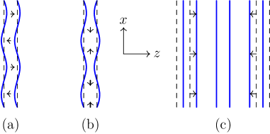
Figure 1: Illustration of different types of deformations leading to a change of Coulomb and surface energies in the lasagne phase. The small arrows indicate the displacement field $\boldsymbol{\mathrm{\xi}}$. (a) spatially varying shear in the $xz$ plane (cf. Eq. (25)), (b) compression by displacing protons inside the lasagne plates ($B_{11}$ term in Eq. (20)), (c) compression by changing the distance between the plates ($B_{33}$ term in Eq. (20)).

and (c). The energy can now be written in the form

$$\delta\mathscr{V}_{\mathrm{C+S},1}=\frac{B_{11}}{2}(\partial_{x}\xi_{x}+\partial_{y}\xi_{y})^{2}+B_{13}(\partial_{x}\xi_{x}+\partial_{y}\xi_{y})(\partial_{z}\xi_{z})\\ +\frac{B_{33}}{2}(\partial_{z}\xi_{z})^{2}\,,$$ (20)

with

$$B_{11}=\tfrac{4}{3}(1-6u+6u^{2})C_{0}\,,$$ (21)

$$B_{13}=\tfrac{4}{3}(-1+2u^{2})C_{0}\,,$$ (22)

$$B_{33}=\tfrac{4}{3}u^{2}C_{0}\,,$$ (23)

where we have introduced the abbreviation

$$C_{0}=\pi e^{2}\bar{n}_{p}^{2}R_{\mathrm{WS}}^{2}\,.$$ (24)

Our result differs from the one given in LABEL:Pethick1998 where only the first term of Eq. (19) was taken into account. Note that the combination $K_{\mathrm{C+S}}=(4B_{11}+4B_{13}+B_{33})/9$ represents a (negative) correction to the bulk modulus, but it is much smaller than the contribution of the electrons, $K$.

From the particular geometry of the lasagne phase it is clear that shear deformations in the $xy$ plane do not change the energy. As noticed in LABEL:Pethick1998, spatially constant shear deformations in the $xz$ (or $yz$) plane contribute only at fourth order in their amplitude (terms $\propto(\partial_{x}\xi_{z})^{4}$ etc.). However, spatially varying shear deformations in the $xz$ (or $yz$) plane (cf. Fig. 1(a)) contribute already at second order in the amplitude. The corresponding energy can be written as Pethick and Potekhin (1998)

$$\delta\mathscr{V}_{\mathrm{C+S},2}=\frac{K_{1}}{2}(\partial_{x}^{2}\xi_{z}+\partial_{y}^{2}\xi_{z})^{2}\,,$$ (25)

To find the coefficient $K_{1}$, one considers, e.g., a displacement field $\xi_{z}=\xi_{0}\cos kx$, and calculates the change in energy to second order in $\xi_{0}$. The $k^{2}\xi_{0}^{2}$ terms coming from the Coulomb and the surface energies cancel, and the leading non-vanishing term is proportional to $k^{4}\xi_{0}^{2}$. The coefficient of this term can be identified with $K_{1}/4$, and one obtains Pethick and Potekhin (1998)

$$K_{1}=\tfrac{4}{45}\pi e^{2}\bar{n}_{p}^{2}R_{\mathrm{WS}}^{4}(1-u)^{2}(1+2u-2u^{2})\,.$$ (26)

III.4.2 Spaghetti phase

Now let us discuss the spaghetti phase. The exact calculation of the Coulomb energy is quite involved in this case, but, except for the energy due to shear deformations in the $xy$ plane, we may use the Wigner-Seitz approximation as a first estimate: the unit cell in the $xy$ plane, which is a rhombus with side length $L$ and angle $60\degree$, is replaced by a circle of radius $R_{\mathrm{WS}}$ with the same area (i.e., $R_{\mathrm{WS}}=3^{1/4}L/\sqrt{2\pi}$). In this approximation, the Coulomb energy is readily calculated. The sum of Coulomb and surface energies per volume is

$$\varepsilon_{\mathrm{C+S}}=\frac{\pi}{2}e^{2}n_{p,2}^{2}R_{\mathrm{WS}}^{2}u^{2}(-1+u-\ln u)+\frac{2\sqrt{u}\sigma}{R_{\mathrm{WS}}}\,.$$ (27)

Again, the condition $\partial\varepsilon_{\mathrm{C+S}}/\partial R_{\mathrm{WS}}=0$ allows one to express $\sigma$ in terms of the equilibrium values of $n_{p,2}$, $u$, and $R_{\mathrm{WS}}$. The calculation of the energy variation under dilatations in the plane perpendicular to the rods ($xy$) or in the direction of the rods ($z$) is completely analogous to the case of the lasagne phase (in Fig. 1 one only has to exchange $x$ and $z$ directions). In the spaghetti phase, one has $\delta u=-u\boldsymbol{\mathrm{\nabla}}\cdot\boldsymbol{\mathrm{\xi}}$ and $\delta R_{\mathrm{WS}}=\frac{1}{2}R_{\mathrm{WS}}\boldsymbol{\mathrm{\nabla}}_{\perp}\boldsymbol{\mathrm{\xi}}_{\perp}$ (with $\boldsymbol{\mathrm{\xi}}_{\perp}$ and $\boldsymbol{\mathrm{\nabla}}_{\perp}$ the projections of $\boldsymbol{\mathrm{\xi}}$ and $\boldsymbol{\mathrm{\nabla}}$ onto the $xy$ plane). Inserting Eq. (27) into Eq. (19), the energy change is again of the form of Eq. (20), only the coefficients are different:

$$B_{11}=\tfrac{1}{4}(-2+4u)C_{0}\,,$$ (28)

$$B_{13}=\tfrac{1}{4}(-4+6u)C_{0}\,,$$ (29)

$$B_{33}=\tfrac{1}{4}(-9+11u-3\ln u)C_{0}\,.$$ (30)

Analogous to the case of the lasagne phase, a constant shear deformation in the $xz$ (or $yz$) plane does not change the energy at second order in the amplitude, but a shear deformation that oscillates as a function of $z$ does. The corresponding energy is now written in the form Pethick and Potekhin (1998)

$$\delta\mathscr{V}_{\mathrm{C+S},2}=\frac{K_{3}}{2}(\partial_{z}^{2}\boldsymbol{\mathrm{\xi}}_{\perp})^{2}\,.$$ (31)

To find the coefficient $K_{3}$, we follow again LABEL:Pethick1998 and calculate the Coulomb energy for cylindrical spaghetti arranged in a hexagonal lattice, which are displaced by $\boldsymbol{\mathrm{\xi}}=\boldsymbol{\mathrm{\xi}}_{0}\cos kz$ ($\boldsymbol{\mathrm{\xi}}_{0}$ lying in the $xy$ plane):

$$\varepsilon_{C}=\frac{8\pi e^{2}n_{p,2}^{2}u}{R_{\mathrm{WS}}^{2}}\sideset{}{{}^{\prime}}{\sum}_{lmn}\frac{[J_{n}(\boldsymbol{\mathrm{k}}_{lm}\cdot\boldsymbol{\mathrm{\xi}}_{0})J_{1}(k_{lm}R)]^{2}}{k_{lm}^{2}(k_{lm}^{2}+n^{2}k^{2})}\,.$$ (32)

The prime indicates that the term $l=m=n=0$ is excluded. The $\boldsymbol{\mathrm{k}}_{lm}=l\boldsymbol{\mathrm{b}}_{1}+m\boldsymbol{\mathrm{b}}_{2}$ are reciprocal lattice vectors, $\boldsymbol{\mathrm{b}}_{1}$ and $\boldsymbol{\mathrm{b}}_{2}$ have length $b=3^{-1/4}\sqrt{8\pi}/R_{\mathrm{WS}}$ and the angle between them is $60\degree$, such that $k_{lm}^{2}=b^{2}(l^{2}+m^{2}+lm)$. To find $K_{3}$, we expand Eq. (32) in $k$ and $\boldsymbol{\mathrm{\xi}}_{0}$ and retain only the term $\propto k^{4}\xi_{0}^{2}$, since the term $\propto k^{2}\xi_{0}^{2}$ must be cancelled by the surface energy. Only the terms $n=\pm 1$ contribute and we obtain

$$K_{3}\approx\frac{e^{2}n_{p,2}^{2}R_{\mathrm{WS}}^{4}u}{32\sqrt{3}\pi^{2}}\left(27[J_{1}(3^{-1/4}\sqrt{8\pi u})]^{2}\right.\\ +\left.[J_{1}(3^{1/4}\sqrt{8\pi u})]^{2}+\cdots\right)\,,$$ (33)

where we have kept only the largest and second largest terms in the sum over $l$ and $m$ since the sum converges extremely well.

Let us now turn to the shear modulus for shear in the $xy$ plane, which was of course absent in the lasagne phase while in the spaghetti phase it exists. The corresponding energy can be written as

$$\delta\mathscr{V}_{\mathrm{C+S},3}=\frac{C_{66}}{2}\left[(\partial_{x}\xi_{x}-\partial_{y}\xi_{y})^{2}+(\partial_{y}\xi_{x}+\partial_{x}\xi_{y})^{2}\right]\,.$$ (34)

The invariance of the hexagonal lattice under rotations by $60\degree$ implies that the same elastic constant $C_{66}$ appears in front of the two terms. To obtain $C_{66}$, we again have to start from the exact expression of the Coulomb energy, but now for a finite shear $\partial_{y}\xi_{x}\equiv\xi_{xy}$ which changes the reciprocal lattice vectors into $\boldsymbol{\mathrm{b}}_{1}^{\prime}=\boldsymbol{\mathrm{b}}_{1}$ and $\boldsymbol{\mathrm{b}}_{2}^{\prime}=\boldsymbol{\mathrm{b}}_{2}+(\sqrt{3}\xi_{xy}/2)\boldsymbol{\mathrm{b}}_{1}$ (we choose the coordinate system such that $\boldsymbol{\mathrm{b}}_{1}$ points in $y$ direction). Then the Coulomb energy becomes

$$\varepsilon_{C}=\frac{8\pi e^{2}n_{p,2}^{2}u}{R_{\mathrm{WS}}^{2}}\sideset{}{{}^{\prime}}{\sum}_{lm}\frac{[J_{1}(k^{\prime}_{lm}R)]^{2}}{k^{\prime\,4}_{lm}}$$ (35)

with $\boldsymbol{\mathrm{k}}^{\prime}_{lm}=l\boldsymbol{\mathrm{b}}^{\prime}_{1}+m\boldsymbol{\mathrm{b}}^{\prime}_{2}$. Expanding this expression up to order $\xi_{xy}^{2}$, keeping only the quadratic term, and using the invariance of the lattice under rotations by multiples of $60\degree$, one eventually obtains (see Appendix A)

$$C_{66}=2\pi e^{2}n_{p,2}^{2}u^{2}\sum_{lm}\Big{(}\frac{[J_{2}(k_{lm}R)]^{2}}{k^{2}_{lm}}\\ +\frac{4J_{1}(k_{lm}R)J_{2}(k_{lm}R)}{k_{lm}^{3}R}-\frac{[J_{1}(k_{lm}R)]^{2}}{k^{2}_{lm}}\Big{)}\,.$$ (36)

As explained in Appendix A, one can rewrite this sum as an integral in coordinate space which can be done analytically, with the result

$$C_{66}=\tfrac{1}{4}C_{0}\,.$$ (37)

So far, the elastic coefficients have been calculated without screening of the Coulomb interaction by the electrons. In order to include this effect, one has to replace $k_{lm}^{2}+n^{2}k^{2}$ in the denominator of Eq. (32) by $k_{lm}^{2}+n^{2}k^{2}+k_{\mathrm{TF}}^{2}$, with $k_{\mathrm{TF}}^{2}=(4e^{2}/\pi)(3\pi^{2}n_{e})^{2/3}$. Repeating the steps described before, performing the remaining summations over $l$ and $m$ numerically, we found that the screening effect is weak and may be neglected. We note also that our analytical results (33) and (37) agree with the numerical results shown in Fig. 2 of LABEL:Pethick1998.

III.4.3 Crystalline phase

Finally, let us consider the crystalline phase. For a cubic crystal, there are only three independent elastic constants, say, $C_{11}$, $C_{12}$, and $C_{44}$ Ashcroft and Mermin (1976). The combination $(C_{11}+2C_{12})/3$ is the bulk modulus and we assume that it is dominated by the electron contribution $K$ discussed in Sec. III.3 so that the Coulomb contribution to it can be neglected. The energy due to shear deformations is written as

$$\delta\mathscr{V}_{\mathrm{C+S}}=\frac{C_{11}-C_{12}}{2}\sum_{i=x,y,z}\left(\partial_{i}\xi_{i}-\frac{\boldsymbol{\mathrm{\nabla}}\cdot\boldsymbol{\mathrm{\xi}}}{3}\right)^{2}\\ +C_{44}\sum_{i\neq j}\left(\frac{\partial_{i}\xi_{j}+\partial_{j}\xi_{i}}{2}\right)^{2}\,.$$ (38)

The constants $C_{11}-C_{12}$ and $C_{44}$ were calculated, e.g., in Refs. Fuchs (1936); Ogata and Ichimaru (1990):

$$C_{11}-C_{12}=0.06545\,C_{0}\,,\quad C_{44}=0.2437\,C_{0}\,.$$ (39)

Screening corrections to these numbers were computed in LABEL:Baiko2015, but in the inner crust they are weak.

From Eq. (39) one sees that the anisotropy of the BCC crystal is very strong (an isotropic material has $C_{11}-C_{12}=2C_{44}$). Since the crust is probably a polycrystal made of many crystallites having random orientations, one often uses an effective shear modulus obtained by a suitable averaging Kobyakov and Pethick (2015). This procedure seems very reasonable for the description of macroscopic phenomena such as vibrations of the star, but it is probably not adequate for the description of phonons whose wavelength we assume to be large compared to the lattice constant $L$ but not necessarily large compared to the size of the crystallites. We therefore keep the anisotropic form of Eq. (38), as we did for the pasta phases, where the same argument applies.

IV Lagrangian density

IV.1 Lagrangian density for pure neutron matter

Before writing the Lagrangian density describing the inner crust of neutron stars, let us consider as a pedagogical example the simpler case of pure neutron matter. In terms of the phase $\varphi$ as degree of freedom, the Lagrangian of a one-component superfluid reads Son and Wingate (2006) (see also Greiter et al. (1989))

$$\mathscr{L}=P\left(\mu_{n}^{(0)}-\dot{\varphi}-\frac{(\boldsymbol{\mathrm{\nabla}}\varphi)^{2}}{2m}\right)\,,$$ (40)

where $P(\mu_{n})$ is the pressure of neutron matter und $\mu_{n}$ the chemical potential. The superscript $(0)$ indicates equilibrium quantities.

The conjugate momentum to the field $\varphi$ is given by $\partial\mathscr{L}/\partial\dot{\varphi}=-\partial P/\partial\mu_{n}=-n_{n}$, so that the Hamiltonian takes the expected form

$$\mathscr{H}=-n_{n}\dot{\varphi}-\mathscr{L}=\varepsilon-\mu^{(0)}n_{n}+\frac{n_{n}^{(0)}}{2m}(\boldsymbol{\mathrm{\nabla}}\varphi)^{2}+\cdots\,,$$ (41)

where the dots stand for terms of third or higher order in $\varphi$ that will be neglected, and we have used $P=\mu_{n}n_{n}-\varepsilon$.

In the notation of Sec. III, we could write $\mathscr{H}=\mathscr{V}+\mathscr{T}$. The Lagrangian, however, would not be given by $\mathscr{T}-\mathscr{V}$, but by $\mathscr{L}=P^{(0)}-n_{n}^{(0)}\dot{\varphi}+\delta\mathscr{V}-\mathscr{T}$. There is a linear term, which does not contribute to the equations of motion, and the roles of $\mathscr{T}$ and $\mathscr{V}$ are exchanged, because the kinetic energy $\mathscr{T}$ contains only spatial derivatives of $\varphi$ while the time derivatives of $\varphi$ enter the potential energy $\mathscr{V}$.

IV.2 Lagrangian density for the inner crust

Now we want to write down the Lagrangian for the inner crust in terms of the fields $\bar{\varphi}$ and $\boldsymbol{\mathrm{\xi}}$. As we have seen in the example of pure neutron matter, the Lagrangian is not given by $\mathscr{T}-\mathscr{V}$. Therefore we start from the Hamiltonian which we write as $\mathscr{H}=\mathscr{H}^{(0)}+\mathscr{T}+\delta\mathscr{V}$, with $\mathscr{T}$ and $\delta\mathscr{V}$ from Sec. III, replacing $\boldsymbol{\mathrm{u}}_{n}=\boldsymbol{\mathrm{\nabla}}\bar{\varphi}/m$, $\boldsymbol{\mathrm{u}}_{p}=\dot{\boldsymbol{\mathrm{\xi}}}$, and $\delta\mu_{n}=-\dot{\bar{\varphi}}$. As before, we keep only terms up to second order in the deviations from equilibrium. A Lagrangian that corresponds to this Hamiltonian is given by

$$\mathscr{L}=-\mathscr{H}^{(0)}+\frac{\Gamma}{2}\dot{\bar{\varphi}}^{2}-\frac{1}{2m}(\boldsymbol{\mathrm{\nabla}}\bar{\varphi})\cdot\underline{\boldsymbol{\mathrm{n}}}_{n}^{s}\boldsymbol{\mathrm{\nabla}}\bar{\varphi}-\dot{\bar{\varphi}}\boldsymbol{\mathrm{\nabla}}\cdot\underline{\boldsymbol{\mathrm{\alpha}}}\boldsymbol{\mathrm{\xi}}\\ +\frac{m}{2}\dot{\boldsymbol{\mathrm{\xi}}}\cdot(\underline{\boldsymbol{\mathrm{n}}}_{n}^{b}+\bar{n}_{p}\underline{\boldsymbol{\mathrm{I}}})\dot{\boldsymbol{\mathrm{\xi}}}-\delta\mathscr{V}_{e}-\delta\mathscr{V}_{\mathrm{C+S}}\,.$$ (42)

To this Lagrangian, one could add a term $\propto\dot{\bar{\varphi}}$ as it was present in pure neutron matter, but such a term does not affect the equations of motion. Furthermore, one could add a term $\dot{\boldsymbol{\mathrm{\xi}}}\cdot\underline{\boldsymbol{\mathrm{\beta}}}\boldsymbol{\mathrm{\nabla}}\bar{\varphi}$, but up to total derivatives such a term can be absorbed in the term $-\dot{\bar{\varphi}}\boldsymbol{\mathrm{\nabla}}\cdot\underline{\boldsymbol{\mathrm{\alpha}}}\boldsymbol{\mathrm{\xi}}$ already present in Eq. (42).

In order to determine $\underline{\boldsymbol{\mathrm{\alpha}}}$, one has to use an additional information, namely the conservation of the neutron number, which can be expressed as a continuity equation

$$\delta\dot{\bar{n}}_{n}+\boldsymbol{\mathrm{\nabla}}\cdot\left(\underline{\boldsymbol{\mathrm{n}}}_{n}^{s}\frac{\boldsymbol{\mathrm{\nabla}}\bar{\varphi}}{m}+\underline{\boldsymbol{\mathrm{n}}}_{n}^{b}\dot{\boldsymbol{\mathrm{\xi}}}\right)=0\,.$$ (43)

From Eq. (10), one has $\delta\bar{n}_{n}=-\Gamma\dot{\bar{\varphi}}+\gamma_{p}\bar{n}_{p}\boldsymbol{\mathrm{\nabla}}\cdot\boldsymbol{\mathrm{\xi}}$. Inserting now the equation of motion

$$\left(\frac{\partial\mathscr{L}}{\partial\dot{\bar{\varphi}}}\right)^{\!\!\!\mbox{$\cdot$}}+\boldsymbol{\mathrm{\nabla}}\cdot\frac{\partial\mathscr{L}}{\partial(\boldsymbol{\mathrm{\nabla}}\bar{\varphi})}=\Gamma\ddot{\bar{\varphi}}-\boldsymbol{\mathrm{\nabla}}\cdot\left(\underline{\boldsymbol{\mathrm{\alpha}}}\dot{\boldsymbol{\mathrm{\xi}}}+\underline{\boldsymbol{\mathrm{n}}}_{n}^{s}\frac{\boldsymbol{\mathrm{\nabla}}\bar{\varphi}}{m}\right)=0\,,$$ (44)

one finds

$$\underline{\boldsymbol{\mathrm{\alpha}}}=\gamma_{p}\bar{n}_{p}\underline{\boldsymbol{\mathrm{I}}}+\underline{\boldsymbol{\mathrm{n}}}_{n}^{b}\,.$$ (45)

The term $-\dot{\bar{\varphi}}\boldsymbol{\mathrm{\nabla}}\cdot\underline{\boldsymbol{\mathrm{\alpha}}}\boldsymbol{\mathrm{\xi}}$ generalizes the mixing term introduced by Cirigliano et al. Cirigliano et al. (2011) for the isotropic case (cubic crystal), in which it reduces to $-\alpha\dot{\bar{\varphi}}\boldsymbol{\mathrm{\nabla}}\cdot\boldsymbol{\mathrm{\xi}}$. Our $\alpha$ corresponds to $f_{\phi}\sqrt{\rho}g_{\text{mix}}$ in the notation of LABEL:Cirigliano2011. There, its value was determined by imposing gauge invariance, which is equivalent to imposing the validity of the continuity equation. In Eq. (62) of LABEL:Cirigliano2011, our factor $\gamma_{p}$, which is defined in the simplified model of constant densities in both phases with a sharp interface, is replaced by the more general expression $(\partial\bar{n}_{n}/\partial\bar{n}_{p})_{\mu_{n}}$.

V Results

In order to obtain the phonon dispersion relations, we write down the Euler-Lagrange equations, i.e., Eq. (44) and the analogous equations of motion for the components of $\boldsymbol{\mathrm{\xi}}$,

$$\left(\frac{\partial\mathscr{L}}{\partial\dot{\xi_{i}}}\right)^{\!\!\!\mbox{$\cdot$}}+\sum_{j}\partial_{j}\frac{\partial\mathscr{L}}{\partial(\partial_{j}\xi_{i})}-\sum_{jk}\partial_{j}\partial_{k}\frac{\partial\mathscr{L}}{\partial(\partial_{j}\partial_{k}\xi_{i})}=0\,.$$ (46)

Assuming $\bar{\varphi}=\bar{\varphi}_{0}e^{i(\boldsymbol{\mathrm{k}}\cdot\boldsymbol{\mathrm{r}}-\omega t)}$ and $\boldsymbol{\mathrm{\xi}}=\boldsymbol{\mathrm{\xi}}_{0}e^{i(\boldsymbol{\mathrm{k}}\cdot\boldsymbol{\mathrm{r}}-\omega t)}$, one can reduce the problem to an algebraic matrix equation (see Appendix B). For a given wave vector $\boldsymbol{\mathrm{k}}$, it is straight-forward to find the eigenvalues $\omega_{i}(\boldsymbol{\mathrm{k}})$ and the corresponding eigenvectors $(\bar{\varphi}_{0i},\boldsymbol{\mathrm{\xi}}_{0i})$.

V.1 Lasagne phase

Because of the invariance of the lasagne phase with respect to rotations around the $z$ axis, one may consider without loss of generality the case $k_{x}=k\sin\theta$, $k_{y}=0$, and $k_{z}=k\cos\theta$. Furthermore, since the lasagne phase does not support any shear stress in the $xy$ plane, a transverse mode having $\boldsymbol{\mathrm{\xi}}$ in $y$ direction has $\omega=0$. It is therefore sufficient to consider only the degrees of freedom $\bar{\varphi}$, $\xi_{x}$ and $\xi_{z}$, and there are only three eigenmodes with $\omega>0$.

In Fig. 2,

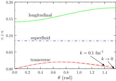
Figure 2: Angle dependence of the velocities of the three phonons in the lasagne phase (parameters see Table 1).

Table 1: Parameters used in Figs. 2–6 (from the Extended Thomas-Fermi (ETF) calculation of LABEL:Martin2015).

		lasagne	spaghetti	BCC crystal
$\rho_{B}$	(g/cm3)	$1.27\cdot 10^{14}$	$1.06\cdot 10^{14}$	$9.87\cdot 10^{13}$
$n_{B}$	(fm-3)	0.0767	0.0640	0.0595
$R_{\mathrm{WS}}$	(fm)	9.94	12.75	14.86
$R$	(fm)	3.90	5.63	8.05
$n_{n,1}$	(fm-3)	0.0644	0.0541	0.0505
$n_{n,2}$	(fm-3)	0.0890	0.0938	0.0950
$n_{p,2}$	(fm-3)	0.0075	0.0128	0.0146

we show the corresponding three sound velocities $v_{i}=\omega_{i}/k$ as functions of the angle $\theta$. The two higher modes are mixed. Nevertheless one can say that in first approximation the highest mode corresponds to the longitudinal lattice phonon, i.e., the displacement $\boldsymbol{\mathrm{\xi}}$ is approximately parallel to $\boldsymbol{\mathrm{k}}$. Its velocity depends essentially on $K$ and $\underline{\boldsymbol{\mathrm{n}}}_{n}^{b}$ and the angle dependence reflects the anisotropy of $\underline{\boldsymbol{\mathrm{n}}}_{n}^{b}$. The second mode is the superfluid phonon (i.e., the eigenvector is dominated by $\bar{\varphi}$). Its angle dependence is surprisingly weak. It turns out that this is the result of a compensation between the effect of the angle dependence of the kinetic energy term and the one of the anisotropic mixing with the longitudinal lattice phonon. Finally, the lowest-lying phonon is a transverse wave. Without the term $\propto K_{1}$ in Eq. (25), its energy would be approximately proportional to $k\sin 2\theta$. With the term $\propto K_{1}$, however, its energy for $\theta=90\degree$ remains finite and proportional to $k^{2}$, i.e., the sound velocity $v$ depends on $k$. This is why we show results for two different values of $k$.

We can compute the contribution of each mode $i$ to the specific heat,

$$c_{v,i}=\frac{\partial}{\partial T}\int_{\text{BZ}}\frac{d^{3}k_{\perp}}{(2\pi)^{3}}\frac{\omega_{i}(\boldsymbol{\mathrm{k}})}{e^{\omega_{i}(\boldsymbol{\mathrm{k}})/T}-1}\,,$$ (47)

where we have restricted the $\boldsymbol{\mathrm{k}}$ integral to the first Brillouin zone (BZ). In the lasagne phase, this means that we integrate $k_{x}$ and $k_{y}$ from $-\infty$ to $+\infty$ but restrict the $k_{z}$ integral to $|k_{z}|<\pi/L=\pi/(2R_{\mathrm{WS}})$. The results are shown in Fig. 3.

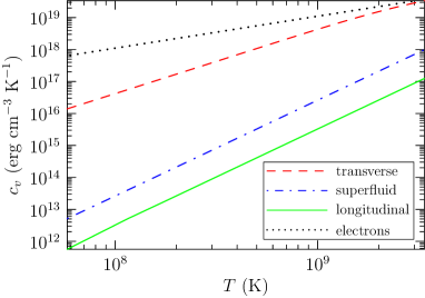
Figure 3: Temperature dependence of the contributions to the specific heat of the lasagne phase corresponding to the three phonons shown in Fig. 2. For comparison, the electron contribution $c_{v,e}=\mu_{e}^{2}T/3$ is also shown.

The specific heat is dominated by the mode which has the lowest velocity, i.e., the transverse phonon. Furthermore, because of its complicated angle-dependent dispersion relation, this mode gives rise to a specific heat proportional to $T^{2}$ at low temperatures, in contrast to the usual $T^{3}$ behavior of the other two contributions. Notice that a $T^{2}$ behavior of the specific heat in the lasagne phase was already found in Refs. Di Gallo et al. (2011); Urban and Oertel (2015), however, the angle dependence of the mode was different there. In any case, up to $T=3\cdot 10^{9}$ K, the electron contribution to $c_{v}$, which is linear in $T$, is dominant.

Notice that, if there was not the term $\propto K_{1}$ that gives a finite energy to the transverse phonon at $\theta=90\degree$, its contribution to the specific heat would diverge. Therefore, $c_{v}$ depends sensitively on the value of $K_{1}$. Furthermore, $c_{v}$ depends also sensitively on the cut-off $\pi/(2R_{\mathrm{WS}})$ of the $k_{z}$ integral. This is a problem since in principle the effective theory can be assumed to be reliable only at $k\ll 1/R_{\mathrm{WS}}$ and it is therefore not clear whether one can trust the dispersion relations $\omega(\boldsymbol{\mathrm{k}})$ up to $k=\pi/(2R_{\mathrm{WS}})$.

V.2 Spaghetti phase

Although the hexagonal lattice of the spaghetti phase has only a discrete rotational invariance, the effective Lagrangian is invariant under rotations around the $z$ axis and we may again assume $k_{x}=k\sin\theta$, $k_{y}=0$, and $k_{z}=k\cos\theta$ without loss of generality. But unlike the lasagne phase, the spaghetti phase supports shear stress in the $xy$ plane and we have therefore a fourth mode, namely a transverse mode with $\boldsymbol{\mathrm{\xi}}$ in $y$ direction, which is decoupled from the other three modes.

The corresponding four sound velocities are displayed in Fig. 4.

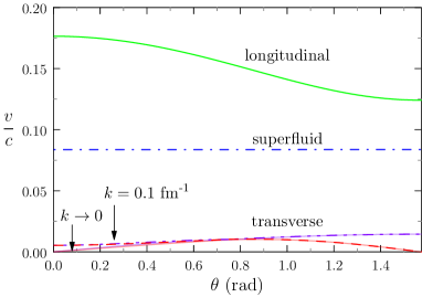
Figure 4: Angle dependence of the velocities of the four phonons in the spaghetti phase. The parameters are given in Table 1.

The two lower modes are transverse lattice phonons, while the two upper modes are the coupled longitudinal lattice phonon and the superfluid phonon. Note that, for $\theta=0$, both transverse modes are degenerate with $\omega=\sqrt{\smash[b]{K_{3}/[m(n_{n,xx}^{b}+\bar{n}_{p})]}}k^{2}$, i.e., a $k$ dependent velocity. In the other limiting case, $\theta=90\degree$, only the transverse mode with $\boldsymbol{\mathrm{\xi}}$ in $y$ direction survives (because of the finite shear modulus $C_{66}$), while the energy of the second transverse mode goes to zero since a $z$ independent displacement field in $z$ direction does not produce any restoring force.

In Fig. 5

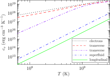
Figure 5: Temperature dependence of the contributions to the specific heat of the spaghetti phase corresponding to the four phonons shown in Fig. 4.

we display the temperature dependence of the corresponding specific heat $c_{v}$. In this case, the first BZ extends from $-\infty$ to $\infty$ in $z$ direction while in the $xy$ plane it is a hexagon with side length $b/\sqrt{3}$, which we approximate by a circle with the same area, i.e., with radius $k_{\perp\max}=2/R_{\mathrm{WS}}$. Again, the dominant contribution to the heat capacity comes from the low-lying transverse modes. Because of their different angle dependence, these contributions behave very differently. The contribution of the mode with $\boldsymbol{\mathrm{\xi}}$ in the $xz$ plane (or generally, in the plane spanned by $\boldsymbol{\mathrm{k}}$ and the $z$ axis) is linear in $T$ and about one half of the electron contribution, while the contribution of the mode with $\boldsymbol{\mathrm{\xi}}$ in $y$ direction (or perpendicular to the plane spanned by $\boldsymbol{\mathrm{k}}$ and the $z$ axis) is much smaller and behaves like $T^{5/2}$ at low temperature. The contributions of the coupled longitudinal lattice phonon and superfluid phonon are proportional to $T^{3}$ and can be practically neglected in the temperature range of interest.

Note, however, that the warning given at the end of Sec. V.2 applies also here.

V.3 BCC crystal

In the BCC crystal, we have, as in the spaghetti phase, four modes. Although they are in principle all coupled with one another (because of the anisotropy), the two lowest ones are essentially transverse lattice phonons and only weakly coupled with the two higher ones corresponding to the mixed longitudinal lattice phonon and superfluid phonon. Now the speeds of sound depend on the polar angle $\theta$ and on the azimuthal angle $\phi$. In Fig. 6

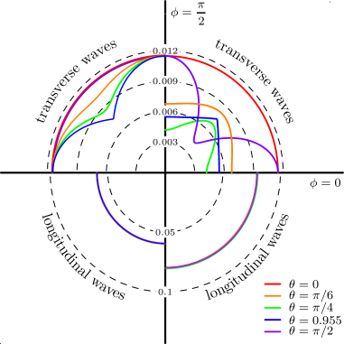
Figure 6: Dependence of the velocities of the four phonons in the BCC crystal on the azimuthal angle $\phi$ for five different values of the polar angle: $\theta=0$, $30\degree$, $45\degree$, $54.7\degree$, and $90\degree$, corresponding to $\cos\theta=1$, $\sqrt{3}/2$, $1/\sqrt{2}$, $1/\sqrt{3}$, and $0$, respectively. The speeds of sound are indicated by the radial distance of the curves from the origin. Note that the scales are different for the transverse (upper scale) and longitudinal (lower scale) modes. The parameters are given in Table 1.

we show as an example the $\phi$ dependence of the phonon velocities for different angles $\theta$. Again, the transverse phonons have a much lower velocity than the longitudinal ones. The angle dependence of the transverse modes is very strong, while that of the longitudinal modes is in practice negligible.

In contrast to the lasagne and spaghetti phases, in the crystal all phonon velocities are already at leading order ($\omega\propto k$) non-vanishing for all angles. Therefore, it is not necessary to include higher-order terms (such as $\delta\mathscr{V}_{\mathrm{C+S},2}$) in the Lagrangian. Also, the calculation of the specific heat is simplified since, at low temperatures where the effective theory can be assumed to be valid, one may take the integral in Eq. (47) over the whole $\boldsymbol{\mathrm{k}}$ space instead of the first BZ. Then one finds

$$c_{v,i}=\frac{2\pi^{2}T^{3}}{15\langle v_{i}\rangle^{3}}$$ (48)

if the mode velocity is angle averaged in a suitable way as

$$\langle v_{i}\rangle=\left(\int\!\frac{d\Omega}{4\pi}\,\frac{1}{v_{i}^{3}}\right)^{-1/3}\,,$$ (49)

where $v_{i}=\omega_{i}(\boldsymbol{\mathrm{k}})/k$ is the (angle dependent) phonon velocity and $\Omega$ is the solid angle. The four angle-averaged mode frequencies are displayed in Fig. 7

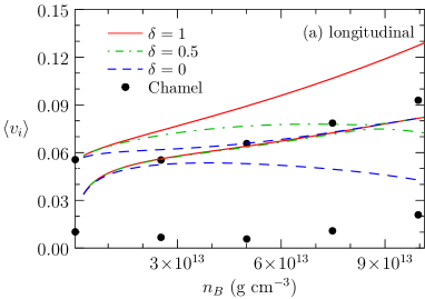
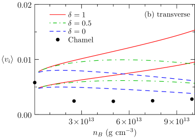
Figure 7: Density dependence of the angle-averaged velocities of the four phonons in the crystalline phase: (a) longitudinal waves, (b) transverse waves. The solid lines ($\delta=1$) correspond to the superfluid hydrodynamic model for the entrainment, Eq. (2), while the dashed lines ($\delta=0.5$, $0$) take into account a possible reduction of the superfluid density inside the clusters (cf. Eq. (50)). The density dependence of the parameters ($R,R_{\mathrm{WS}},n_{n,i},n_{p,2}$) of the crust were taken from the ETF calculation of LABEL:Martin2015. The points are the results of LABEL:Chamel2013.

as the solid lines.

Compared with LABEL:Chamel2013, except for the highest mode, for which the agreement is reasonable, the phonon velocities are generally much higher in our model. The reason for this discrepancy is that in the hydrodynamic model, the suppression of the superfluid neutron density $n_{n}^{s}$ due to entrainment is much weaker and therefore $n_{n}^{b}$ is smaller than in the band-structure calculation Chamel (2012) used in LABEL:Chamel2013. This results in higher phonon velocities which are roughly proportional to $(n_{n}^{b}+\bar{n}_{p})^{-1/2}$ (except for the superfluid phonon), see Appendix B.3. If we artificially replace our $n_{n}^{s}/\bar{n}_{n}=1-n_{n}^{b}/\bar{n}_{n}$ from Eq. (2) by the numerical results of LABEL:Chamel2012, we obtain a reasonable agreement with the phonon velocities shown in LABEL:Chamel2013 in spite of our slightly different crust composition.

The weaker entrainment found in the hydrodynamic model allows one to solve some problems with the description of glitches Martin and Urban (2016). It also goes into the same direction as a recent study based on a completely different approach Watanabe and Pethick (2017). Nevertheless, one might question the validity of the hydrodynamic approach because the coherence length, especially inside the clusters, is not small enough compared to the cluster size. To account for this problem in a pragmatic way, in LABEL:Martin2016 a parameter $0\leq\delta\leq 1$ was introduced which characterizes the fraction of effectively superfluid neutrons inside the clusters in the sense that the microscopic neutron current inside the cluster is given by $\delta\,n_{n,2}\boldsymbol{\mathrm{\nabla}}\phi/m+(1-\delta)n_{n,2}\boldsymbol{\mathrm{v}}_{p}$ instead of $n_{n,2}\boldsymbol{\mathrm{\nabla}}\phi/m$. Then, the entrainment increases (although it remains always weaker than that of LABEL:Chamel2012) and the expression (2) for $n_{n}^{b}$ is replaced by

$$n_{n}^{b}=un_{n,2}\Big{(}1-\delta+\frac{(\delta-\gamma)^{2}}{(2\gamma+\delta)}\Big{)}\,.$$ (50)

In the limiting case $\delta\to 0$ (i.e., all neutrons inside the clusters flow together with the protons and the neutron gas has to flow around the clusters), one recovers the result obtained in LABEL:Sedrakian1996.

The results discussed so far correspond to the case $\delta=1$. In Fig. 7, we also display results obtained for $\delta=0.5$ and $\delta=0$ (dashed lines). With decreasing $\delta$, the phonon velocities become smaller, getting somewhat closer to the results of LABEL:Chamel2013. As in LABEL:Chamel2013, we see an avoided crossing of the longitudinal lattice phonon and the superfluid phonon due to the mixing term. Note that the heat capacity goes like $1/v^{3}$, so that the remaining uncertainty of the phonon velocities may change the specific heat by a huge factor.

VI Conclusion

Generalizing the ideas of LABEL:Cirigliano2011 to the pasta phases, we have constructed the Lagrangian density of an effective theory describing the long-wavelength dynamics of the inner crust in terms of the coarse-grained variables $\bar{\varphi}$ and $\boldsymbol{\mathrm{\xi}}$. Also in the pasta phases, there is a mixing term between lattice and superfluid phonons, which is now anisotropic, i.e., angle dependent.

To determine the parameters of the effective theory, we have used the superfluid hydrodynamics approach of LABEL:Martin2016 for the kinetic energy including the entrainment, and the phase-coexistence model for the strong-interaction contribution to the potential energy. The incompressibility of the lattice comes essentially from the electron gas. Coulomb and surface energies are responsible for the elastic properties of the lattice, which we have revisited in detail, mainly following LABEL:Pethick1998. But we allow also for compression due to motion in the direction of the pasta, without change of the distance between pasta structures [see Fig. 1(b)], which was not considered in LABEL:Pethick1998.

We have then applied the effective theory to compute the phonon velocities and specific heats of the lasagne, spaghetti, and BCC crystal phases. The angle dependence of the phonon velocities is very strong in all three phases. In the pasta phases, certain transverse phonon velocities even become equal to zero for $\theta=0$ or $90\degree$, leading to a qualitative change in the behavior of the specific heat at low temperatures, as already noticed in Refs. Di Gallo et al. (2011); Urban and Oertel (2015). In particular, in the spaghetti phase, the contribution of one of the transverse phonons to the specific heat is linear in $T$ and about one half of the electron contribution.

The largest uncertainty comes probably from the entrainment parameters. The superfluid hydrodynamics approach used here predicts a much weaker entrainment than the band-structure calculation used in LABEL:Chamel2013. Therefore, our phonon velocities in the crystalline phase are higher than those of LABEL:Chamel2013. Since a full so-called Quasiparticle Random-Phase Approximation (QRPA) calculation is only feasible in a WS cell Khan et al. (2005); Inakura and Matsuo (2017) but not in the periodic structure of the inner crust, the superfluid hydrodynamics approach should be cross-checked with the QRPA in the WS cell.

Note that in the present work, as in Refs. Di Gallo et al. (2011); Martin and Urban (2016), we have neglected the microscopic entrainment related to the dependence of the microscopic neutron effective mass inside the cluster on the proton density (and vice versa) Borumand et al. (1996). However, this effect seems to be rather weak Urban and Oertel (2015).

In the present work, questions related to phonon damping were not addressed, but they are important in the context of the phonon contribution to the heat conductivity Ashcroft and Mermin (1976). Phonon damping arises from their coupling to electrons Kobyakov et al. (2017), whose dynamics is not yet fully treated, from the phonon scattering off impurities and from processes involving more than two phonons Page and Reddy (2012). To describe the phonon-phonon coupling, one has to include terms into the effective Lagrangian involving terms of higher order in the fields $\bar{\varphi}$ and $\boldsymbol{\mathrm{\xi}}$.

Finally we note that in the stage of finalizing the present manuscript, a very similar study by Kobyakov and Pethick appeared Kobyakov and Pethick (2018).

Appendix A Evaluation of the sums in the hexagonal lattice

We consider the hexagonal lattice defined by $\boldsymbol{\mathrm{r}}_{lm}=l\boldsymbol{\mathrm{a}}_{1}+m\boldsymbol{\mathrm{a}}_{2}$, with $\boldsymbol{\mathrm{a}}_{1}=L\boldsymbol{\mathrm{e}}_{x}$ and $\boldsymbol{\mathrm{a}}_{2}=(L/2)\boldsymbol{\mathrm{e}}_{x}+(\sqrt{3}L/2)\boldsymbol{\mathrm{e}}_{y}$, and $\boldsymbol{\mathrm{e}}_{i}$ the unit vector in direction $i$. The unit cell $A$ is the rhombus defined by the vectors $\boldsymbol{\mathrm{a}}_{1}$ and $\boldsymbol{\mathrm{a}}_{2}$ and has an area of $|A|=\sqrt{3}L^{2}/2=\pi R_{\mathrm{WS}}^{2}$. The reciprocal lattice is given by the vectors $\boldsymbol{\mathrm{k}}_{lm}$ defined below Eq. (32), with $\boldsymbol{\mathrm{b}}_{1}=b\boldsymbol{\mathrm{e}}_{y}$ and $\boldsymbol{\mathrm{b}}_{2}=-(\sqrt{3}b/2)\boldsymbol{\mathrm{e}}_{x}+(b/2)\boldsymbol{\mathrm{e}}_{y}$. A function $f(\boldsymbol{\mathrm{r}})$ ($\boldsymbol{\mathrm{r}}$ denotes here a two-component vector in the $xy$ plane) having the periodicity of this lattice can be expanded in a Fourier series $f(\boldsymbol{\mathrm{r}})=\sum_{lm}f_{\boldsymbol{\mathrm{k}}_{lm}}e^{i\boldsymbol{\mathrm{k}}_{lm}\cdot\boldsymbol{\mathrm{r}}}$, with $f_{\boldsymbol{\mathrm{k}}_{lm}}=(1/|A|)\int_{A}d^{2}rf(\boldsymbol{\mathrm{r}})e^{-i\boldsymbol{\mathrm{k}}_{lm}\cdot\boldsymbol{\mathrm{r}}}$. We will also make use of the relation

$$|A|\sum_{lm}f_{\boldsymbol{\mathrm{k}}_{lm}}g_{-\boldsymbol{\mathrm{k}}_{lm}}=\int_{A}d^{2}rf(\boldsymbol{\mathrm{r}})g(\boldsymbol{\mathrm{r}})\,.$$ (51)

The lattice is symmetric with respect to rotations by $60\degree$. Such a rotation changes the indices $m$ and $l$ according to $(l,m)\mapsto(-m,l+m)$. For a given pair $(l,m)$, let us denote by $(l^{(n)},m^{(n)})$ the indices one obtains by successively applying $n$ such rotations, in particular $(l^{(0)},m^{(0)})=(l^{(6)},m^{(6)})=(l,m)$. Suppose one wants to sum a term $a_{lm}$ over $l$ and $m$. Then one can write

$$\sum_{lm}a_{lm}=\sum_{lm}\frac{1}{6}\sum_{n=0,5}a_{l^{(n)}m^{(n)}}\equiv\sum_{lm}a^{(\text{symm})}_{lm}$$ (52)

in order to make the symmetry already apparent before the summation is performed. This trick has been used to obtain the compact formula for $C_{66}$ in Eq. (36).

Consider now the functions

$$f_{1}(\boldsymbol{\mathrm{r}})=\theta(R-r)\,,\quad f_{2}(\boldsymbol{\mathrm{r}})=r_{x}\theta(R-r)\,,\\ f_{3}(\boldsymbol{\mathrm{r}})=(R^{2}-r^{2})\theta(R-r)$$ (53)

and their Fourier transforms

$$f_{1,\boldsymbol{\mathrm{k}}}=\frac{2R}{R_{\mathrm{WS}}^{2}}\,\frac{J_{1}(kR)}{k}\,,\quad f_{2,\boldsymbol{\mathrm{k}}}=\frac{2iR^{2}}{R_{\mathrm{WS}}^{2}}\,\frac{k_{x}J_{2}(kR)}{k^{2}}\,,\\ f_{3,\boldsymbol{\mathrm{k}}}=\frac{4R^{2}}{R_{\mathrm{WS}}^{2}}\,\frac{J_{2}(kR)}{k^{2}}\,.$$ (54)

Using Eq. (51) with $f=g=f_{1}$, we find

$$\sum_{lm}\frac{[J_{1}(k_{lm}R)]^{2}}{k_{lm}^{2}}=\frac{R_{\mathrm{WS}}^{2}}{4}\,.$$ (55)

Similarly, with $f=f_{1}$, $g=f_{3}$ we obtain

$$\sum_{lm}\frac{J_{1}(k_{lm}R)J_{2}(k_{lm}R)}{k_{lm}^{3}}=\frac{R_{\mathrm{WS}}^{2}R}{16}\,.$$ (56)

With $f=g=f_{2}$ and using Eq. (52) with $[(k_{lm})_{x}^{2}]^{\text{(symm)}}=k_{lm}^{2}/2$, we obtain

$$\sum_{lm}\frac{[J_{2}(k_{lm}R)]^{2}}{k_{lm}^{2}}=\frac{R_{\mathrm{WS}}^{2}}{8}\,.$$ (57)

These equations allow us to transform Eq. (36) into Eq. (37).

Appendix B Matrices

Assuming $\bar{\varphi}=\bar{\varphi}_{0}e^{i(\boldsymbol{\mathrm{k}}\cdot\boldsymbol{\mathrm{r}}-\omega t)}$ and $\boldsymbol{\mathrm{\xi}}=\boldsymbol{\mathrm{\xi}}_{0}e^{i(\boldsymbol{\mathrm{k}}\cdot\boldsymbol{\mathrm{r}}-\omega t)}$, one can write the Euler-Lagrange equations (44) and (46) in matrix form as follows:

$$\left(\begin{smallmatrix}\vphantom{\dot{\xi}_{y}}\omega&1&0&0&0&0&0&0\\ \vphantom{\dot{\xi}_{y}}A_{21}&\omega&0&A_{24}&0&A_{26}&0&A_{28}\\ \vphantom{\dot{\xi}_{y}}0&0&\omega&1&0&0&0&0\\ \vphantom{\dot{\xi}_{y}}0&A_{42}&A_{43}&\omega&A_{45}&0&A_{47}&0\\ \vphantom{\dot{\xi}_{y}}0&0&0&0&\omega&1&0&0\\ \vphantom{\dot{\xi}_{y}}0&A_{62}&A_{63}&0&A_{65}&\omega&A_{67}&0\\ \vphantom{\dot{\xi}_{y}}0&0&0&0&0&0&\omega&1\\ \vphantom{\dot{\xi}_{y}}0&A_{82}&A_{83}&0&A_{85}&0&A_{87}&\omega\end{smallmatrix}\right)\left(\begin{smallmatrix}\vphantom{\dot{\xi}_{y}}-\bar{\varphi}\\ \vphantom{\dot{\xi}_{y}}i\dot{\bar{\varphi}}\\ \vphantom{\dot{\xi}_{y}}-\xi_{x}\\ \vphantom{\dot{\xi}_{y}}i\dot{\xi}_{x}\\ \vphantom{\dot{\xi}_{y}}-\xi_{y}\\ \vphantom{\dot{\xi}_{y}}i\dot{\xi}_{y}\\ \vphantom{\dot{\xi}_{y}}-\xi_{z}\\ \vphantom{\dot{\xi}_{y}}i\dot{\xi}_{z}\end{smallmatrix}\right)=0.$$ (58)

B.1 Lasagne phase

Assuming without loss of generality that $\boldsymbol{\mathrm{k}}$ lies in the $xz$ plane, the matrix elements $A_{ij}$ for the lasagne phase read:

$$A_{21} =\tfrac{\bar{n}_{n}}{\Gamma m}k_{x}^{2}+\tfrac{n_{n,zz}^{s}}{\Gamma m}k_{z}^{2}\,, A_{24} =\tfrac{\gamma_{p}\bar{n}_{p}}{\Gamma}k_{x}\,,$$

$$A_{26} =0\,, A_{28} =\tfrac{n_{n,zz}^{b}+\gamma_{p}\bar{n}_{p}}{\Gamma}k_{z}\,,$$

$$A_{42} =\tfrac{\gamma_{p}}{m}k_{x}\,, A_{43} =\tfrac{K+B_{11}}{m\bar{n}_{p}}k_{x}^{2}\,,$$

$$A_{45} =0\,, A_{47} =\tfrac{K+B_{13}}{m\bar{n}_{p}}k_{x}k_{z}\,,$$

$$A_{62} =0\,, A_{63} =0\,,$$

$$A_{65} =0\,, A_{67} =0\,,$$

$$A_{82} =\tfrac{n_{n,zz}^{b}+\gamma_{p}\bar{n}_{p}}{m(n_{n,zz}^{b}+\bar{n}_{p})}k_{z}\,, A_{83} =\tfrac{(K+B_{13})}{m(n_{n,zz}^{b}+\bar{n}_{p})}k_{x}k_{z}\,,$$

$$A_{85} =0\,, A_{87} =\tfrac{(K+B_{33})k_{z}^{2}+K_{1}k_{x}^{4}}{m(n_{n,zz}^{b}+\bar{n}_{p})}\,.$$ (59)

B.2 Spaghetti phase

Again, we may assume without loss of generality that $\boldsymbol{\mathrm{k}}$ lies in the $xz$ plane. Then the matrix elements $A_{ij}$ for the spaghetti phase read:

$$A_{21} =\tfrac{n_{n,xx}^{s}}{\Gamma m}k_{x}^{2}+\tfrac{\bar{n}_{n}}{\Gamma m}k_{z}^{2}\,, A_{24} =\tfrac{n_{n,xx}^{b}+\gamma_{p}\bar{n}_{p}}{\Gamma}k_{x}\,,$$

$$A_{26} =0\,, A_{28} =\tfrac{\gamma_{p}\bar{n}_{p}}{\Gamma}k_{z}\,,$$

$$A_{42} =\tfrac{n_{n,xx}^{b}+\gamma_{p}\bar{n}_{p}}{m(n_{n,xx}^{b}+\bar{n}_{p})}k_{x}\,, A_{43} =\tfrac{(K+B_{11}+C_{66})k_{x}^{2}+K_{3}k_{z}^{4}}{m(n_{n,xx}^{b}+\bar{n}_{p})}\,,$$

$$A_{45} =0\,, A_{47} =\tfrac{K+B_{13}}{m(n_{n,xx}^{b}+\bar{n}_{p})}k_{x}k_{z}\,,$$

$$A_{62} =0\,, A_{63} =0\,,$$

$$A_{65} =\tfrac{C_{66}k_{x}^{2}+K_{3}k_{z}^{4}}{m(n_{n,xx}^{b}+\bar{n}_{p})}\,, A_{67} =0\,,$$

$$A_{82} =\tfrac{\gamma_{p}}{m}k_{z}\,, A_{83} =\tfrac{K+B_{13}}{m\bar{n}_{p}}k_{x}k_{z}\,,$$

$$A_{85} =0\,, A_{87} =\tfrac{K+B_{33}}{m\bar{n}_{p}}k_{z}^{2}\,.$$ (60)

B.3 Crystalline phase

In the crystal, we have to allow for a general $\boldsymbol{\mathrm{k}}$ with components $k_{x}$, $k_{y}$, and $k_{z}$:

$$A_{21} =\tfrac{n_{n}^{s}}{\Gamma m}(k_{x}^{2}+k_{y}^{2}+k_{z}^{2})\,, A_{24} =\tfrac{n_{n}^{b}+\gamma_{p}\bar{n}_{p}}{\Gamma}k_{x}\,,$$

$$A_{26} =\tfrac{n_{n}^{b}+\gamma_{p}\bar{n}_{p}}{\Gamma}k_{y}\,, A_{28} =\tfrac{n_{n}^{b}+\gamma_{p}\bar{n}_{p}}{\Gamma}k_{z}\,,$$

$$A_{42} =\tfrac{n_{n}^{b}+\gamma_{p}\bar{n}_{p}}{m(n_{n}^{b}+\bar{n}_{p})}k_{x}\,, A_{43} =\tfrac{C_{12}k_{x}^{2}+C_{44}(k_{y}^{2}+k_{z}^{2})}{m(n_{n}^{b}+\bar{n}_{p})}\,,$$

$$A_{45} =\tfrac{C_{11}+C_{44}}{m(n_{n}^{b}+\bar{n}_{p})}k_{x}k_{y}\,, A_{47} =\tfrac{C_{11}+C_{44}}{m(n_{n}^{b}+\bar{n}_{p})}k_{x}k_{z}\,,$$

$$A_{62} =\tfrac{n_{n}^{b}+\gamma_{p}\bar{n}_{p}}{m(n_{n}^{b}+\bar{n}_{p})}k_{y}\,, A_{63} =\tfrac{C_{11}+C_{44}}{m(n_{n}^{b}+\bar{n}_{p})}k_{x}k_{y}\,,$$

$$A_{65} =\tfrac{C_{12}k_{y}^{2}+C_{44}(k_{x}^{2}+k_{z}^{2})}{m(n_{n}^{b}+\bar{n}_{p})}\,, A_{67} =\tfrac{C_{11}+C_{44}}{m(n_{n}^{b}+\bar{n}_{p})}k_{y}k_{z}\,,$$

$$A_{82} =\tfrac{n_{n}^{b}+\gamma_{p}\bar{n}_{p}}{m(n_{n}^{b}+\bar{n}_{p})}k_{z}\,, A_{83} =\tfrac{C_{11}+C_{44}}{m(n_{n}^{b}+\bar{n}_{p})}k_{x}k_{z}\,,$$

$$A_{85} =\tfrac{C_{11}+C_{44}}{m(n_{n}^{b}+\bar{n}_{p})}k_{y}k_{z}\,, A_{87} =\tfrac{C_{12}k_{z}^{2}+C_{44}(k_{x}^{2}+k_{y}^{2})}{m(n_{n}^{b}+\bar{n}_{p})}\,.$$ (61)

References

- Chamel and Haensel (2008) N. Chamel and P. Haensel, Living Rev. Relativ. 11, 10 (2008).
- Ravenhall et al. (1983) D. G. Ravenhall, C. J. Pethick, and J. R. Wilson, Phys. Rev. Lett. 50, 2066 (1983).
- Page and Reddy (2012) D. Page and S. Reddy, Neutron Star Crust (Nova Science Publishers, Hauppage, 2012), chap. 14, eprint 1201.5602.
- Cirigliano et al. (2011) V. Cirigliano, S. Reddy, and R. Sharma, Phis. Rev. C 84, 045809 (2011).
- Martin and Urban (2016) N. Martin and M. Urban, Phys. Rev. C 94, 065801 (2016).
- Fuchs (1936) K. Fuchs, Proc. R. Soc. London A 153, 622 (1936).
- Pethick and Potekhin (1998) C. J. Pethick and A. Y. Potekhin, Phys. Lett. B 427, 7 (1998).
- Martin and Urban (2015) N. Martin and M. Urban, Phys. Rev. C 92, 015803 (2015).
- Pethick et al. (2010) C. J. Pethick, N. Chamel, and S. Reddy, Progress of theoretical physics Supplement 186, 9 (2010).
- Kobyakov et al. (2017) D. N. Kobyakov, C. J. Pethick, S. Reddy, and A. Schwenk, Phys. Rev. C 96, 025805 (2017).
- Chamel and Carter (2006) N. Chamel and B. Carter, Mon. Not. R. Astron. Soc. 368, 796 (2006).
- Magierski (2004) P. Magierski, Int. J. Mod. Phys. E 13, 371 (2004).
- Magierski and Bulgac (2004a) P. Magierski and A. Bulgac, Acta Phys. Polon. B 35, 1203 (2004a).
- Magierski and Bulgac (2004b) P. Magierski and A. Bulgac, Nucl. Phys. A 738, 143 (2004b).
- Kobyakov and Pethick (2016) D. Kobyakov and C. J. Pethick, Phys. Rev. C 94, 055806 (2016).
- Chabanat et al. (1998) E. Chabanat, P. Bonche, P. Haensel, J. Meyer, and R. Schaeffer, Nuclear Physics A 635, 231 (1998).
- Kobyakov and Pethick (2013) D. Kobyakov and C. J. Pethick, Phys. Rev. C 87, 055803 (2013).
- Ashcroft and Mermin (1976) N. W. Ashcroft and N. D. Mermin, Solid State Physics (Saunders, Fort Worth, 1976).
- Ogata and Ichimaru (1990) S. Ogata and S. Ichimaru, Phys. Rev. A 42, 4867 (1990).
- Baiko (2015) D. A. Baiko, Mon. Not. R. Astron. Soc. 451, 3055 (2015).
- Kobyakov and Pethick (2015) D. Kobyakov and C. J. Pethick, Mon. Not. R. Astron. Soc.: Lett. 449, L110 (2015).
- Son and Wingate (2006) D. T. Son and M. Wingate, Ann. Phys. (N.Y.) 321, 197 (2006).
- Greiter et al. (1989) M. Greiter, F. Wilczek, and E. Witten, Mod. Phys. Lett. B 3, 903 (1989).
- Di Gallo et al. (2011) L. Di Gallo, M. Oertel, and M. Urban, Phys. Rev. C 84, 045801 (2011).
- Urban and Oertel (2015) M. Urban and M. Oertel, Int. J. Mod. Phys. E 24, 1541006 (2015).
- Chamel et al. (2013) N. Chamel, D. Page, and S. Reddy, Phys. Rev. C 87, 035803 (2013).
- Chamel (2012) N. Chamel, Phys. Rev. C. 85, 035801 (2012).
- Watanabe and Pethick (2017) G. Watanabe and C. J. Pethick, Phys. Rev. Lett. 119, 062701 (2017).
- Sedrakian (1996) A. Sedrakian, Astrophysics and Space Science 236, 267 (1996).
- Khan et al. (2005) E. Khan, N. Sandulescu, and N. V. Giai, Phys. Rev. C 71, 042801 (2005).
- Inakura and Matsuo (2017) T. Inakura and M. Matsuo, Phys. Rev. C 96, 025806 (2017).
- Borumand et al. (1996) M. Borumand, R. Joynt, and W. Kluźniak, Phys. Rev. C 54, 2745 (1996).
- Kobyakov and Pethick (2018) D. N. Kobyakov and C. J. Pethick, Preprint (2018), eprint arXiv:1803.06254.