Structural and Dynamical Properties of Galaxies in a Hierarchical Universe: Sizes and Specific Angular Momenta

Abstract

We use a state-of-the-art semi-analytic model to study the size and the specific angular momentum of galaxies. Our model includes a specific treatment for the angular momentum exchange between different galactic components. Disk scale radii are estimated from the angular momentum of the gaseous/stellar disk, while bulge sizes are estimated assuming energy conservation. The predicted size–mass and angular momentum–mass relations are in fair agreement with observational measurements in the local Universe, provided a treatment for gas dissipation during major mergers is included. Our treatment for disk instability leads to unrealistically small radii of bulges formed through this channel, and predicts an offset between the size–mass relations of central and satellite early-type galaxies, that is not observed. The model reproduces the observed dependence of the size–mass relation on morphology, and predicts a strong correlation between specific angular momentum and cold gas content. This correlation is a natural consequence of galaxy evolution: gas-rich galaxies reside in smaller halos, and form stars gradually until present day, while gas-poor ones reside in massive halos, that formed most of their stars at early epochs, when the angular momentum of their parent halos is low. The dynamical and structural properties of galaxies can be strongly affected by a different treatment for stellar feedback, as this would modify their star formation history. A higher angular momentum for gas accreted through rapid mode does not affect significantly the properties of massive galaxies today, but has a more important effect on low-mass galaxies at higher redshift.

1 Introduction

The history of a galaxy (and of its components) is determined by a network of physical processes that drive a complex exchange of mass, energy, metals and angular momentum. In a hierarchical Universe, galaxies are believed to form from the collapse of baryons in the potential well of Dark Matter (DM) halos. These acquire their angular momentum through gravitational tidal torques during the growth of perturbations (Peebles, 1969; White, 1984; Barnes & Efstathiou, 1987). Numerical simulations show that the gas and dark matter within virialized systems have very similar initial angular momentum distributions (in agreement with standard assumptions, Fall & Efstathiou, 1980), although there is a slight misalignment between their angular momentum vectors (van den Bosch et al., 2002; van den Bosch et al., 2003; Sharma & Steinmetz, 2005).

As hot gas cools, preserving its angular momentum, a rotationally supported cold gas disk forms. Star formation takes place within overdense regions of this cold gas disk, originating a stellar disk that is assumed to inherit the angular momentum of the cold gas from which it forms. A spheroidal component (a bulge) can form through galaxy–galaxy mergers (Barnes & Hernquist, 1991; Katz, 1992; Hopkins et al., 2010), or through dynamical instabilities in disk galaxies (see Kormendy & Kennicutt, 2004, and references therein). The former channel is believed to originate classical and kinetically hot spheroids, while the latter is believed to lead to the formation of the so-called ‘pseudo-bulges’ that are dynamically cold and have Sérsic indices, stellar populations and velocity dispersions intermediate between those of classical bulges and disks (Andredakis & Sanders, 1994; de Jong, 1996; Peletier & Balcells, 1996; Carollo et al., 2001; MacArthur et al., 2003; Kormendy & Kennicutt, 2004; Drory & Fisher, 2007). Therefore, the observed structure and dynamical properties of galaxies are intimately connected to the evolution of the gas angular momentum.

Progress on the observational side has recently allowed a systematic study of the sizes and angular momenta for statistical samples of galaxies. High resolution imaging in several photometric bands became available from e.g. the Sloan Digital Sky Survey (SDSS, York et al. 2000) or the Galaxy And Mass Assembly (GAMA, Driver et al. 2011) project in the local Universe, and e.g. CANDELS (Grogin et al., 2011) at higher redshift. The advent of Integral Field Spectroscopy allowed measurements of spatially resolved properties for thousands of galaxies, starting with the pioneering work done with SAURON (Bacon et al., 2001) and culminating in ongoing projects like CALIFA, SAMI, and MaNGA (Sánchez et al., 2012; Bryant et al., 2015; Bundy et al., 2015).

The first analysis of the size–mass relation based on a statistical sample of galaxies was carried out by Shen et al. (2003), using SDSS data. The observed relation exhibits a large scatter that depends on the morphology of the galaxies, with Late Type (LT) galaxies having, on average, larger characteristic radii than Early Types (ETs) at fixed stellar mass. Different ET/LT selections lead to similar size–mass median relations (e.g. Lange et al., 2015, based on GAMA). Satellite LT galaxies are slightly smaller than centrals, while the size of ET galaxies does not appear to be significantly affected by the environment (e.g. Weinmann et al., 2009; Huertas-Company et al., 2013, both based on SDSS). The sizes of both LT and ET galaxies tend to decrease with increasing redshift (Ichikawa et al., 2012; van der Wel et al., 2014).

The first attempt to study the relation between the specific angular momentum ($j_{*}$) and galaxy stellar mass ($M_{*}$) was made by Fall (1983), for a small sample of galaxies of different morphological types. Romanowsky & Fall (2012) extended the original analysis using different techniques (including long slit spectroscopy, integrated stellar light spectroscopy, and extended PN kinematics) to extrapolate the rotational profile of LT and ET galaxies out to large aperture radii (from $\sim 2$ to $\sim 8\,R_{eff}$). They used these results to formulate an empirical relation to infer the total specific angular momentum from measurements limited to $\sim 2$ half-light radii, and applied this empirical formula to a larger sample of galaxies. This study showed that, as for the sizes, the scatter in the $j_{*}$–$M_{*}$ relation depends on galaxy morphology. Recently, spatially resolved velocity maps have become available for hundreds of galaxies. Data from the ATLAS^3D project (Cappellari et al., 2011) revealed that ET galaxies exhibit a complex internal dynamical structure. ET galaxies are classified as ‘fast’ or ‘slow’ rotators according to the importance of the rotational velocity compared to the velocity dispersion, respectively. This classification has been connected to different galaxy assembly histories: fast rotators originate predominantly from secular evolution, while slow rotators are associated with recent and numerous accretion events (Davis et al., 2011; Serra et al., 2014; Davis & Bureau, 2016). Obreschkow & Glazebrook (2014) used a small sample of gas-rich spiral galaxies from THINGS (Walter et al., 2008), and showed that they lie on a plane in the 3D space described by the specific angular momentum, the stellar mass, and the bulge over total mass ratio. An estimate of the $j_{*}$–$M_{*}$ relation for both LT and ET galaxies has been recently provided by Cortese et al. (2016), based on SAMI data (Bryant et al., 2015). In the near future, it will be possible to extend these studies to even larger mass selected samples of galaxies using e.g. data from MaNGA (Bundy et al., 2015).

Many theoretical studies have focused on the origin of both galaxy sizes and their specific angular momenta in a cosmological context. The analytic framework was laid out in early studies (Fall & Efstathiou, 1980; Dalcanton et al., 1997; Mo et al., 1998), which have provided the basis for most of the published semi-analytic work on the subject. First hydrodynamical simulations suffered from excessive loss of angular momentum, resulting in too compact galaxies compared to the observational measurements (Steinmetz & Navarro, 1999; Navarro & Steinmetz, 2000). The origin of this problem was identified in the excessive cooling (and star formation) during the early phases of galaxy formation, which was due to a combination of limited numerical resolution and stellar feedback implementation (Weil et al., 1998; Eke et al., 2000; Abadi et al., 2003; Governato et al., 2004). In more recent years, many groups have succeeded in reproducing realistic thin disks supported by rotation (Governato et al., 2010; Guedes et al., 2011; Danovich et al., 2015; Murante et al., 2015). Recent studies also focused on the origin of the specific angular momentum versus stellar mass relation in simulations (Übler et al., 2014; Marinacci et al., 2014; Teklu et al., 2015; Genel et al., 2015; Zavala et al., 2016; DeFelippis et al., 2017; Sokołowska et al., 2017; Grand et al., 2017). These groups have shown that strong feedback at high redshift is crucial to remove low angular momentum gas and produce galaxy disks with sizes and rotational properties comparable to those measured in the local Universe (Übler et al., 2014). Numerical work has also shown that gas dissipation during galaxy–galaxy mergers plays an important role in determining the sizes and angular momentum of ET galaxies (Hopkins et al., 2009; Hopkins et al., 2014; Porter et al., 2014; Lagos et al., 2018). This has been confirmed by a number of studies relying on semi-analytic models of galaxy formation (Shankar et al., 2013; Tonini et al., 2016). Although most modern models also include a specific treatment for the exchange of angular momentum among the different baryonic components (e.g. Lagos et al., 2009; Guo et al., 2011; Benson, 2012; Tonini et al., 2016; Xie et al., 2017), less attention has been devoted to the specific angular momentum of galaxies in the semi-analytic framework (dedicated studies have been published by Lagos et al. 2015 and Stevens et al. 2016).

In this paper, we will use a state-of-the-art semi-analytic model including prescriptions for angular momentum evolution, to perform a systematic analysis of both size and specific angular momentum distributions of galaxies of different morphological type. The layout of the paper is as follows: in Section 2, we give details about the semi-analytic model used in this work, and about the dark matter simulations employed. In Section 3, we describe the size–mass relation predicted by our model and different variants considered, and we compare it to observational measurements both for LT and ET galaxies. We discuss the stellar specific angular momenta of our model galaxies in Section 4, while in Section 5 we explain the dependence of the predicted relations on morphology, gas content of model galaxies, and specific implementation for gas cooling and stellar feedback. Finally, in Section 6, we discuss our results and give our conclusions.

2 The model

In this work, we take advantage of the GAlaxy Evolution and Assembly (GAEA) semi-analytic model, described in Hirschmann et al. (2016), as updated in Xie et al. (2017). This model descends from that originally published in De Lucia & Blaizot (2007), but many prescriptions have been updated significantly over the past years. In particular, GAEA includes a sophisticated treatment for the non instantaneous recycling of gas, metals, and energy (De Lucia et al., 2014), and a new stellar feedback scheme partly based on results of hydrodynamical simulations (Hirschmann et al., 2016). In this work, we use the GAEA model updated, as described in Xie et al. (2017), to include a specific treatment for angular momentum exchanges between galactic components, and prescriptions to partition the cold gas into its molecular (star forming) and atomic components. Specifically, we will use the model adopting the Blitz & Rosolowsky (2006) prescription to estimate the molecular gas fraction, and will refer to this implementation as X17. In this work, we also consider several modifications of the standard X17 implementation, as detailed below. A summary of all alternative runs considered is provided in Table 1.

Table 1: Summary of the model runs considered in this work. The second column indicates if/when gas dissipation during mergers is accounted for; the third column lists the proportionality parameter relating the specific angular momentum of the gas accreting in rapid mode to that of the hot gas halo; the fourth column indicates the adopted feedback scheme.

Name	Dissipation	Gas accretion	Feedback Scheme
X17	No	$\alpha_{CA}=1$	FIRE
X17allM	During all mergers	$\alpha_{CA}=1$	FIRE
X17MM	During major mergers	$\alpha_{CA}=1$	FIRE
X17CA3	During major mergers	$\alpha_{CA}=3$	FIRE
X17G11	During major mergers	$\alpha_{CA}=1$	Guo et al. (2011)

Our fiducial model is able to reproduce the observed evolution of the galaxy stellar mass function up to $z\sim 7$ and of the cosmic star formation rate density up to $z\sim 10$ (Fontanot et al., 2017). In addition, the model reproduces the measured correlation between stellar mass/luminosity and metal content of galaxies in the local Universe, down to the scale of Milky Way satellites (De Lucia et al., 2014; Hirschmann et al., 2016), and the evolution of the galaxy mass–gas metallicity relation up to redshift $z\sim 2$ (Hirschmann et al., 2016; Xie et al., 2017). The model is, however, not without problems: in particular, we have shown that massive galaxies tend to form stars at higher rates than observed (Hirschmann et al., 2016), and that the model tends to under-predict the measured level of star formation activity at high redshift (Xie et al., 2017).

In the following, we provide a brief description of the Xie et al. (2017) model, focusing only on those prescriptions that are relevant for this work. For more details, we refer to the original papers by De Lucia et al. (2014), Hirschmann et al. (2016), and Xie et al. (2017).

2.1 The cosmological simulation and the merger tree

The merger trees used in this work are based on the Millennium Simulation (MRI, Springel et al., 2005), and on the higher resolution Millennium II Simulation (MRII, Boylan-Kolchin et al., 2009). The MRI follows the evolution of N=$2160^{3}$ particles of mass $8.6\times 10^{8}h^{-1}{\rm M_{\sun}}$, in a box of $500\;h^{-1}$Mpc comoving on a side. Simulation outputs are stored in 64 snapshots, logarithmically spaced in redshift. The cosmological model adopted is consistent with WMAP1 data (Spergel et al., 2003), with cosmological parameters $\Omega_{b}=0.045$, $\Omega_{m}=0.25$, $\Omega_{\Lambda}=0.75$, $H_{0}=100h\;{\rm Mpc^{-1}\;km\;s^{-1}}$, $h=0.73$, $\sigma_{8}=0.9$, and $n=1$. This cosmology is nowadays out-of-date, and more precise estimates of the cosmological parameters are available from e.g. the PLANCK collaboration (Planck Collaboration et al., 2014). In particular, the most recent estimates converge towards a lower value of $\sigma_{8}\;(=0.829)$. As this parameter heavily influences the clustering of cosmic structures, a different value of $\sigma_{8}$ is expected to affect also the evolution of model galaxies. Previous studies (Wang et al., 2008; Guo et al., 2013) have shown, however, that model results are qualitatively similar when run on a simulation with lower $\sigma_{8}$, although the different cosmology requires a slight retuning of the physical parameters of the model. We do not attempt here to rescale the cosmology of the MR as done, for example, in Guo et al. (2013). Based on previous results, we expect that such modifications would not affect significantly our results.

The halo merger trees used as input for our galaxy formation model are built in different steps. First, halos and sub-halos are identified for each snapshot. Halos are identified using a classical Friends-of-Friends algorithm, with a linking length equal to 0.2 times the mean inter-particle separation. The SUBFIND algorithm (Springel et al., 2001) is then used to identify bound substructures in each FoF halo. As in previous work, we consider as genuine substructures only those with at least 20 particles, which sets the halo mass resolution to $M_{h}=1.7\times 10^{10}h^{-1}{\rm M_{\sun}}$ for the MRI. For each subhalo at any given snapshot, a unique descendant is identified at the subsequent snapshot, by tracing a subset of the most bound particles (Springel et al., 2005). In this way, each subhalo is automatically linked to all its progenitors (at the previous snapshot), i.e. its merger history is defined. For each halo, a main branch is defined as the one that follows, at each node of the tree, the progenitor with the largest integrated mass (De Lucia & Blaizot, 2007).

When necessary, to verify the robustness of our results at masses near the resolution limit of the simulation, we use the MRII. This corresponds to a simulation box with size of $100\;h^{-1}$Mpc on a side (one fifth of the Millennium), with a particle mass that is 125 times smaller than that used in the MRI. This lowers the halo mass resolution to $M_{\rm h}=1.4\times 10^{8}h^{-1}{\rm M_{\sun}}$. The resolution limits of the MRI and MRII simulations translate in stellar mass limits for the X17 model of about $\sim 10^{9}\;{\rm M_{\sun}}$ and $\sim 10^{8}\;{\rm M_{\sun}}$ for the MRI and MRII, respectively (see Fig. 6 of Xie et al., 2017).

2.2 The fiducial semi-analytic model

Our semi-analytic model attaches baryonic components to each simulated halo, considering their merger histories and observationally and/or theoretically motivated prescriptions to model the evolution of the baryons. In this section, we focus on the processes driving the evolution of galaxy sizes and angular momenta, i.e. the main subject of this work.

2.2.1 Cooling

When a halo collapses, it is assigned a hot gas component, and the total baryonic mass in the halo is assumed to be $M_{baryons}=f_{b}M_{200}$ ($f_{b}$ is the universal baryon fraction, and $M_{200}$ is defined as the mass corresponding to an over-density of 200 times the critical density of the Universe). In our model, the hot gas is assumed to follow an isothermal distribution and can cool only onto central galaxies. The process is modeled as described in detail in De Lucia et al. (2010), following the original prescriptions outlined in White & Frenk (1991): a cooling radius is defined as the radius at which the local cooling time is equal to the halo dynamical time. Two different cooling regimes are considered, depending on how the cooling radius compares to the virial radius $R_{200}$ (the radius corresponding to $M_{200}$). At high redshift and for small haloes, the formal cooling radius is much larger than the virial radius. In this case, the infalling gas is not expected to reach hydrostatic equilibrium. Gas accretion is anisotropic (filamentary) and limited by the infall rate. In this ‘rapid cooling regime’ (or ‘cold accretion mode’), we assume that all the hot gas available cools in one code time step. When instead the cooling radius is smaller than the halo virial radius, the hot gas is assumed to reach hydrostatic equilibrium and to cool quasi-statically. In this ‘slow cooling regime’ (or ‘hot accretion mode’), the cooling rate is modeled by a simple inflow equation.

In both regimes, we assume that the hot gas transfers angular momentum to the cold gas disk, proportionally to the cooled mass, $M_{\rm cooling}$. As in previously published models, the hot halo is assumed to have the same specific angular momentum as the dark matter halo $\vec{j}_{\rm DM}$, so that the specific angular momentum of the cold gas after cooling can be written as:

$$\vec{j}_{\rm cold}^{f}=\frac{\vec{j}_{\rm cold}^{0}M_{\rm cold}^{0}+\alpha_{A}\,\vec{j}_{\rm DM}M_{\rm cooling}}{M_{\rm cold}^{0}+M_{\rm cooling}}.$$ (1)

In the above equation, $\vec{j}_{\rm cold}^{f}$ and $\vec{j}_{\rm cold}^{0}$ are the specific angular momenta of the cold gas after and before gas cooling, $M_{\rm cold}^{0}$ is the mass of the cold gas disk before cooling, and $\alpha_{A}$ is assumed to be 1 in our fiducial model. Several recent studies based on hydrodynamical simulations (Stewart et al., 2011; Pichon et al., 2011; Danovich et al., 2015) have shown that, contrary to standard assumptions, gas accreted through cold mode carries a specific angular momentum that is from 2 to 4 times larger than that of the parent DM halo. To quantify the influence of this effect on our model results, we have carried out an alternative run assuming $\alpha_{A}=3$ for gas accreted in the rapid cooling regime. We will refer to this run, which adopts the same model parameters as the reference X17 model, as X17CA3 in the following.

2.2.2 Star formation and stellar feedback

Xie et al. (2017) introduced modified prescriptions for the star formation process, aimed at including an explicit treatment of the atomic-to-molecular gas transition. In our reference X17 model, the total cold gas reservoir associated with each galaxy is partitioned into its molecular and atomic components employing the Blitz & Rosolowsky (2006) empirical relation. The star formation rate is then assumed to depend on the surface density of molecular gas in the disk (Wong & Blitz, 2002; Kennicutt et al., 2007; Leroy et al., 2008).

We assume that the newly formed stars, $M_{*,new}$, carry the angular momentum of the cold gas they originated from. Therefore, after a star formation episode, the specific angular momentum of the stellar disk, $\vec{j}_{*,disk}^{f}$, can be written as:

$$\vec{j}_{\rm*,disk}^{f}=\frac{\vec{j}_{\rm*,disk}^{0}M_{\rm*,disk}^{0}+\vec{j}_{\rm cold}M_{\rm*,new}}{M_{\rm*,disk}^{0}+M_{\rm*,new}},$$ (2)

with $\vec{j}_{\rm*,disk}^{0}$ and $M_{\rm*,disk}^{0}$ representing the specific angular momentum and stellar mass of the disk before star formation, and $\vec{j}_{\rm cold}$ the specific angular momentum of the cold gas disk at the time of star formation. Gas recycled from stars is later returned to the cold gas, carrying the specific angular momentum of the stellar disk or, in the case of gas originating from bulge stars, a zero specific angular momentum.

Stellar feedback injects energy into the interstellar medium, reheating part of the cold gas. In our reference X17 run, the reheating is modeled using parametrizations based on the FIRE hydrodynamical simulations (Hopkins et al., 2014; Muratov et al., 2015). Part of the reheated gas is eventually ejected from the parent halo through galactic winds. The amount of gas ejected is estimated using energy conservation arguments. We assume that reheating and/or ejection does not affect the specific angular momentum of the cold gas and that of the hot gas (the latter is always equal to that of the parent dark matter halo). The ejected gas is stored in a reservoir, from where it can be re-incorporated onto the hot gas associated with the parent halo, on a time-scale that depends on the virial mass of the halo (for a detailed description of the prescriptions adopted for our fiducial stellar feedback scheme, see Hirschmann et al., 2016).

Recent numerical work (Übler et al., 2014; Genel et al., 2015) has highlighted that gas ejected through galactic winds can be accelerated, so that a larger angular momentum is transferred to the disk when the gas is re-accreted. In our model, the ejected gas is not accelerated, but we assume it acquires the same specific angular momentum of the parent halo (which typically increases with increasing cosmic time) before being re-incorporated. To quantify how much our results depend on the feedback scheme adopted, we also consider a different implementation based on the feedback scheme used in Guo et al. (2011). For this particular prescription, we have used the same parameters adopted in Hirschmann et al. (2016), and have not attempted to re-tune them. As shown in our previous work, this feedback scheme does not reproduce, in our GAEA framework, the measured evolution of the galaxy stellar mass function, and implies lower ejection rates of gas at high redshift and shorter re-accretion times with respect to our reference X17 model. This different re-accretion history is expected to affect significantly the star formation history of model galaxies, and therefore also their sizes and angular momenta. In the following, we refer to the run adopting the Guo et al. (2011) stellar feedback parametrization as X17G11.

2.2.3 Bulge formation

Mergers and disk instabilities are the two possible channels that in our model lead to the formation of a bulge. We assume this is a spheroidal component with zero angular momentum, and supported by velocity dispersion.

We distinguish between two types of mergers, based on the baryonic (stars+cold gas) mass ratio between the secondary (less massive) and primary (more massive) merging galaxies. If the mass ratio is larger than 0.3, we assume we have a ‘major merger’ event during which both stellar components of merging galaxies merge into a single remnant bulge. In the case of a minor merger (mass ratio less than 0.3), we assume that the stellar disk of the primary is unperturbed, and that the stars of the secondary are added to the primary bulge. During all mergers, the cold gas of the secondary is added to the cold gas disk of the primary. We assume that the cold gas is first stripped from the satellite, and acquires the same specific angular momentum of the primary dark matter halo, obtaining an equation similar to that used for cooling (Eq. 1), but with the secondary cold gas mass instead of $M_{cooling}$.

We assume that all mergers trigger a star burst in the cold gas disk of the remnant, which is modeled following the ‘collisional starburst’ prescription introduced by Somerville et al. (2001), with coefficients revised using results from Cox et al. (2008). The amount of new stars formed, $M_{*,SB}$, is a fraction of the cold gas of the progenitors, proportional to the merger mass ratio.

Disk instability is modeled as described in detail in Croton et al. (2006, see also ). The instability criterion is based on results by Efstathiou et al. (1982). When a disk becomes unstable, a fraction of stars $\delta M$, necessary to restore the stability, is moved from the central regions of the disk into the bulge. During a disk instability episode, we assume that the angular momentum of the stellar disk is preserved, and thus the specific angular momentum of the disk can be written as:

$$j_{*}^{f}=\frac{j_{*}^{0}M_{*,disk}^{0}}{M_{*,disk}^{0}-\delta M}$$ (3)

with $M_{*,disk}^{0}$ representing the initial mass of the disk before the disk instability event.

As discussed in previous work (see Athanassoula, 2008; Benson & Devereux, 2010; De Lucia et al., 2011; Fontanot et al., 2011), our modeling of disk instability is rather simplified: it does not account, for example, for the possibility that bar formation causes an inflow of gas towards the centre fuelling a starburst, or for violent early disk instability (Elmegreen et al., 2008; Ceverino et al., 2015). In addition, the very same instability criterion adopted has been criticized by e.g. Athanassoula (2008). Improving the modeling adopted for this physical process is highly needed, but goes beyond the aims of this work.

2.2.4 The disk radius and bulge size

In our reference model, the radii of the cold gas and stellar disks are estimated from their specific angular momentum and rotational velocity. Specifically, the disk scale radius is expressed as:

$$R_{x}=\frac{j_{x}}{2V_{max}},$$ (4)

where $R_{x}$ and $j_{x}$ are the radius and the specific angular momentum of the $x$-component (either cold gas or stellar disk). $V_{max}$ is the maximum rotational velocity of the parent halo.

The bulge is assumed to be a dispersion dominated spheroid, and its size is estimated from energy conservation arguments. During mergers of spheroids, the energies involved are those due to their gravitational potential and interaction. Assuming no energy dissipation, we can estimate the energy before the merger as:

$$\begin{split}E_{i}=CG\left[\frac{(M_{*}^{p}+M_{*,SB}^{p})^{2}}{R_{p}}+\frac{(M_{*}^{s}+M_{*,SB}^{s})^{2}}{R_{s}}\right]\\ +\alpha G\frac{(M_{*}^{p}+M_{*,SB}^{p})(M_{*}^{s}+M_{*,SB}^{s})}{R_{p}+R_{s}},\end{split}$$ (5)

and after the merger as:

$$E_{f}=CG\frac{{M_{*}^{f}}^{2}}{R^{f}}.$$ (6)

In the first equation, $G$ is the gravitational constant, $M_{*}^{p}+M_{*,SB}^{p}$ and $M_{*}^{s}+M_{*,SB}^{s}$ are the total stellar masses of the primary ($p$) and the secondary ($s$) galaxy, respectively. $M_{*,SB}$ represents the stars formed during the starburst, and $R_{p}$ and $R_{s}$ are approximations of the half mass radii of the primary and secondary galaxies (including cold gas). The latter are obtained from a mass-weighted average of the sizes of the bulge and disk components. $C=0.5$ is a ‘form factor’, and $\alpha=0.5$ is a parameter accounting for the orbital energy between the spheroids (Cole et al., 2000). In the last equation, $M_{*}^{f}$ is the stellar mass of the remnant spheroid, and $R_{f}$ is its size.

Previous studies have highlighted how this simple treatment leads to unrealistic sizes of galaxies, especially at the low mass end (Hopkins et al., 2009; Covington et al., 2011; Porter et al., 2014). This problem arises from the fact that the model outlined above ignores gas dissipation in bulge formation through mergers. Using high-resolution hydro-simulations, Hopkins et al. (2009) proposed a simple formula to account for gas dissipation, without modifying the energy conservation equation. The final radius can be simply ‘corrected’ as follows:

$$r_{f}=\frac{r_{no\,diss}}{1+f_{gas}/f_{0}}$$ (7)

where $r_{no\,diss}$ represents the bulge size when dissipation is not considered, $f_{gas}$ is the ratio between the gas and the stellar mass involved in the merger (including the stars formed in the associated star-burst), and $f_{0}$ is a parameter varying between $0.25$ and $0.30$. This formula was calculated using a set of controlled simulations of binary mergers with mass ratio larger than 1:6, and the strongest effect was found in the case of disk–disk major mergers (see for example Table 1 in Porter et al., 2014). Therefore, it is not straightforward to apply this correction to all mergers. To understand the impact on our model results, we consider two alternative implementations: we either assume that gas dissipation affects bulge size during all mergers (this run is referred to as X17allM in the following), or we assume that gas dissipation matters only during major mergers (X17MM). In both runs, we assume $f_{0}=0.275$. We have not distinguished mergers between disks from mergers between spheroids (we expect that mergers between spheroids involve typically a small fraction of gas). We also tested an alternative implementation for gas dissipation, which includes a dissipation term in the energy conservation equation during mergers, as proposed by Covington et al. (2011). The results obtained using this alternative implementation are qualitatively similar to those obtained using Eq. 7.

When a disk instability episode occurs, we compute the radius $R_{\delta M}$ enclosing the stellar mass moved from the central part of the disk to the bulge (this is done assuming a disk with an exponential surface density). We then use this radius as the scale-radius of the newly formed spheroidal component. If a bulge already exists, we merge the newly formed spheroid with the pre-existing bulge, assuming energy conservation, as in Eqs. 5 and 6.

3 The size-mass relation

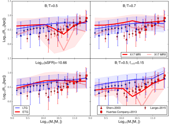
Figure 1: The $R_{1/2}$–$M_{*}$ relation for LT and ET galaxies (blue and red lines) for our reference model X17. Solid lines correspond to results from the MRI, while dashed lines correspond to the MRII. Different panels show different selections for LT and ET galaxies. Shaded areas show the region between the 16th and 84th percentiles of the MRI distribution; we find a similar scatter for the MRII. Symbols with error bars correspond to different observational measurements, as indicated in the legend.

In this section, we study the size–mass relation for model galaxies divided into LT and ET galaxies, and compare model predictions to available observational measurements in the Local Universe. The results of this comparison are shown in Fig. 1, for different LT/ET selections (different panels). Different colors correspond to different galaxy types (red for ET and blue for LT galaxies), while different line styles are used for model results based on the MRI (solid) and on the MRII (dotted lines). The shaded areas indicate the region between the 16th and 84th percentiles of the distribution obtained for the MRI, but a similar scatter is found for the MRII. The sizes shown in the figure correspond to the projected half-mass radii of model galaxies, namely the radii enclosing half of the total stellar mass. To estimate radii for our model galaxies, we assume that all galaxies are seen face-on, an exponential profile for the stars in the disk, and a Jaffe profile for bulge stars (see Appendix A).

Observational estimates are shown in Fig. 1 as symbols with error bars (red and blue are used for ET and LT galaxies, respectively). All the estimates shown correspond to half mass radii, but are based on observations at different wavebands, different assumptions about the light distribution, and different selections for ET and LT galaxies. Shen et al. (2003, triangles) used SDSS data in the $z$-band to estimate Petrosian half-light radii. LT and ET galaxies were classified according to their concentration, with E/S0 galaxies being classified as those with concentration larger than $c=2.86$. Huertas-Company et al. (2013, squares) estimated the half-light radii performing a double component Sérsic fitting for all galaxies from the SDSS DR7 spectroscopic sample, and then selected and studied only ET galaxies taking advantage of a machine learning technique. Lange et al. (2015, stars) estimated the half-light radii along the major axis of GAMA galaxies, using single Sérsic fits. They used elliptical fits, and showed that these give systematically larger radii at fixed stellar mass than the circular fits used in previous studies. They divided LT from ET galaxies using four different methods: a visual morphology classification, a Sérsic index threshold of $n=2.5$, a color–color $(u-r)$–$(g-i)$ division, a combination of Sérsic index and $(u-r)$ color. They found that these different criteria select different galaxy samples, but the size–mass relations obtained are very similar. In this work we use their estimates based on the Sérsic index classification.

In our comparison, we assume that light distribution traces the mass distribution, and we do not attempt to reproduce the ET/LT classification adopted in observational studies to avoid further assumptions. In Fig. 1, we show four different LT/ET selections based on the predominance of the bulge components (in terms of stellar mass) and star formation activity (which generally correlates with the amount of cold gas). In the top panels we consider a simple selection based on the bulge over total stellar mass ratio ($B/T$): specifically, we classify as ET galaxies all those with $B/T>0.5$ or $B/T>0.7$ in the top-left and top-right panel, respectively. In the bottom left panel, we show a selection based on the specific Star Formation Rate (sSFR). The chosen threshold ($\log_{10}({\rm sSFR}\;[{\rm yr^{-1}}])=-10.66$) approximately separates the two peaks of the sSFR distribution of our model galaxies (see Fig. 8 in Hirschmann et al., 2016). As we have noted in our previous work and above, the sSFR distribution predicted by our model does not reproduce well the observed distribution. This problem, however, does not affect the results discussed below qualitatively. Finally, in the bottom right panel of Fig. 1, we show a selection that also considers the cold gas fraction of model galaxies, $f_{\rm cold}=M_{\rm cold}/(M_{\rm cold}+M_{*})$. Specifically, we select as LT galaxies those with $f_{\rm cold}>0.15$ and $B/T<0.5$, and as ET galaxies those with $f_{\rm cold}<0.15$ and $B/T>0.5$. With this selection we are deliberately excluding a relevant number of galaxies, particularly among high mass gas-poor LT galaxies. Nevertheless, we believe that this selection is useful to have a point of comparison with the samples of spiral gas-rich galaxies that are often identified as LT galaxies in observations.

We expect the MRII to provide a more precise estimate of the relation in the stellar mass range $10^{9}-10^{10}\;{\rm M_{\sun}}$, where the MRI is close to its resolution limit. We find that the MRII median size for galaxies with stellar mass $\sim 10^{9}\;{\rm M_{\sun}}$ is about 0.2 dex lower than that based on the MRI, while predictions based on the two simulations are in good agreement at a stellar mass $\sim 10^{10}\;{\rm M_{\sun}}$. At larger stellar masses, since the MRII simulation volume is smaller than that of the MRI, predictions based on this simulation are more noisy. In the following, we will show results from MRII up to a galaxy stellar mass equal to $10^{10}\;{\rm M_{\sun}}$, and results from MRI above this limit.

The predicted size–mass relation for LT galaxies is in nice agreement with measurements by Lange et al. (2015), independently of the selection adopted. As mentioned above, this study adopts elliptical fits rather than circularized ones, and we consider their approach more physical than that adopted in previous studies. In contrast, for ET galaxies, the observed size–mass relation is not well reproduced by any of the selections considered. The two partitions that include a cut at $B/T=0.5$ are in good agreement with data by Shen et al. (2003) and Huertas-Company et al. (2013) for galaxy masses larger than $M_{*}>10^{10.5}\;{\rm M_{\sun}}$. For less massive galaxies, the model significantly over-predicts galaxy sizes. The same holds, over the entire stellar mass range shown, for the other two selections considered. In particular, when selecting galaxies on the basis of the sSFR or using a cut at $B/T=0.7$, model predictions for ET galaxies are very close to those obtained for LT galaxies.

This problem has been noted earlier (Hopkins et al., 2009; Covington et al., 2011; Porter et al., 2014), and is due to the fact that our fiducial model does not include a treatment for dissipation of energy during gas rich mergers.

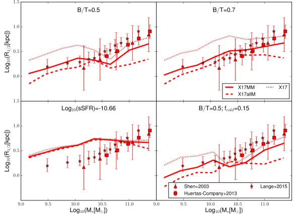
Figure 2: The $R_{1/2}$–$M_{*}$ relation, as in Fig. 1, but for runs including a treatment for gas dissipation in all mergers or in major mergers only (dashed and solid lines, respectively). Predictions from our X17 run are shown as dotted lines, as a reference. As LT galaxies are not affected by the inclusion of gas dissipation, we only show here model predictions and data for ET galaxies.

In Fig. 2, we show the size–mass relation for the X17allM (dashed lines) and for the X17MM (solid lines) runs, which account for dissipation, as in Hopkins et al. (2009). Predictions from our standard model without dissipation are also shown as a reference (dotted lines). LT galaxies are not affected by the inclusion of dissipation, and we do not show their predicted size–mass relation (and the corresponding data) for clarity. For the $B/T=0.5$ and $B/T=0.7$ selections, the inclusion of dissipation lowers the relation, slightly in the case of X17MM and more significantly in the case of X17allM. At the largest masses, where the X17 model is in good agreement with data, both runs including gas dissipation, in particular the X17allM run, predict smaller sizes than the observational estimates. The relation for galaxies selected on the basis of their sSFR is not affected by the introduction of a treatment for gas dissipation. This is due to the fact that many disky galaxies are selected in the passive ET group, keeping the predicted size–mass relation for ET galaxies very close to that predicted by LT galaxies. Finally, the selection including a cut based on $f_{\rm cold}$ results in a relation similar to the division based on $B/T=0.5$. This is expected, because ET galaxies are typically gas poor. Interestingly, dissipation during minor mergers affects significantly the sizes of high mass galaxies ($M_{*}>10^{10.2}\;{\rm M_{\sun}}$). As we will see in Sec. 5, this is due to the fact that these galaxies have experienced many minor mergers during their life.

Since the X17MM run is, among all runs considered here, the one characterized by the best agreement with observational measurements when using selections based on $B/T$, we will adopt this run as our reference model in the rest of the paper.

3.1 The size of galactic components

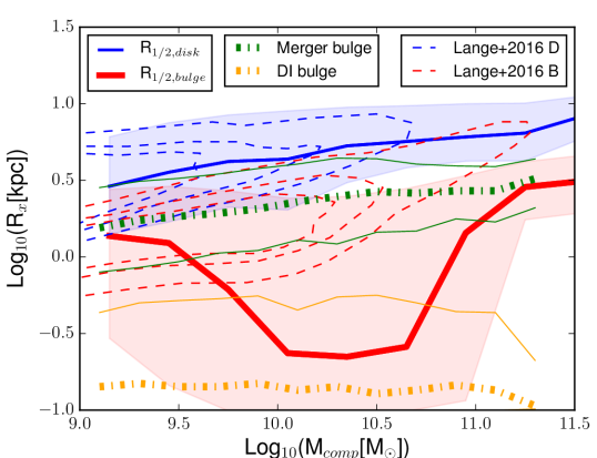
Figure 3: The size–mass relation for the bulge and disk components. The x-axis represents the mass of each component. The thick solid blue and red lines show the median sizes of the stellar disks and of the bulges of model galaxies from our X17MM run. The shaded areas correspond to the region between the 16th and 84th percentiles of the distributions. The green and orange thick dashed-dotted lines show the median relations for merger and disk instability dominated bulges, respectively (see text for details). Thin solid lines of the same colors correspond to the 16th-84th percentiles of the distribution. Finally, the dashed contours show the distributions of observational measurements from Lange et al. (2016), for disks (blue) and spheroids (red).

In this section, we analyze the size–mass relation for the disk and bulge components separately. Fig. 3 shows the half-mass radii versus stellar mass of disks and bulges from the X17MM model, considering all the galaxies. We also show the observed distributions by Lange et al. (2016) as dashed contours (blue for disks and red for spheroids). The median size–mass relation predicted for disks by our X17MM run is in fairly good agreement with observational estimates, while the bulge median relation is offset about 0.5 dex below the observational estimates in the stellar mass range $M_{*}\in[10^{9.8}-10^{11}]\;{\rm M_{\sun}}$. The scatter is large and there is a large overlap between data and model predictions, except at the most massive end, where the model tends to under-predict bulge sizes significantly.

To better understand the behavior of our model, we quantify the relative contribution of mergers and disk instabilities to the mass of each bulge. We then divide model bulges according to the channel that contributed most to their mass: if at least 50% of the bulge mass formed from disk instabilities, it is identified as DI bulge, otherwise it is classified as a merger bulge. The division of bulges into two classes is motivated by observational results (see Kormendy & Kennicutt, 2004, for a review). Recent work has demonstrated that, although characterized by different dynamical properties and radial profiles, these two different bulge families have similar sizes, with pseudo-bulges only slightly larger than classical ones (Gadotti, 2009; Lange et al., 2016). The predicted size–mass relations for DI and merger bulges are shown in Fig. 3 as green and orange solid lines, respectively (thick lines are for the median and thin lines for the 16th-84th percentiles of the distributions). We find that merger bulges are systematically larger than DI bulges, and that their median size–mass relation is only slightly flatter than the observed distribution, especially at high masses. Assuming that all bulges forming primarily through disk instability are ‘pseudo-bulges’, this result is in stark contrast with observational measurements. We will come back to this issue in Sec. 6.2.

3.2 Early type central and satellite galaxies

Observational studies suggest that central and satellite ET galaxies follow the same size–mass relation, at least at the high mass end ($M_{*}>10^{10.5}\;{\rm M_{\sun}}$, see for example Huertas-Company et al., 2013). In Fig. 4, we show the median size–mass relation for all ET galaxies (solid lines) and ET central galaxies only (dashed lines) from the reference X17MM run. LT centrals follow the same relation as all LT galaxies, and we do not show them for clarity.

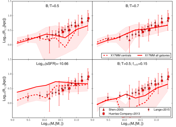
Figure 4: The $R_{1/2}$–$M_{*}$ relation for ET galaxies from the X17MM model. Predictions for all ET galaxies are shown as solid lines, while dashed lines show the average sizes of central ET galaxies only. The shaded areas cover the region enclosed by the 16th and the 84th percentiles of the central galaxies distribution.

The relations found for ET central galaxies are different from the relations found for all ET galaxies, for all the selections considered, except when using a cut at $B/T=0.7$. In the selections assuming a cut at $B/T=0.5$, the size–mass relations predicted for central galaxies are characterized by a strong ‘dip’ in the stellar mass range $M_{*}\in[10^{10}-10^{10.8}]\;{\rm M_{\sun}}$. This dip is not visible when considering all ET galaxies. As explained above, model bulges can form through mergers or disk instabilities, with the latter giving origin, in our model, to rather small bulges. We have verified that, when selecting ET galaxies using $B/T>0.7$, we select bulges formed mainly through mergers (from 93 to 100 per cent depending on the stellar mass range considered). In contrast, selecting ET galaxies with $0.5<B/T<0.7$, we find a significant fraction of bulges formed through disk instability (from 24 to 91 per cent, depending on the mass range). Therefore, bulges formed through disk instabilities contribute significantly to the size–mass relation of samples selected using a $B/T=0.5$.

The results shown in Fig. 4 can, at least in part, be explained by a difference in numbers between centrals and satellites in the stellar mass range $M_{*}\in[10^{10}-10^{10.8}]\;{\rm M_{\sun}}$. Specifically, we find many more centrals in this mass range with $0.5<B/T<0.7$ than with $B/T>0.7$. When considering the entire ET populations, the proportions are inverted, and we find more galaxies with $B/T>0.7$. Therefore, in this mass range, central galaxies include a larger fraction of small bulges than the entire ET population. In Sec. 5.2, we will show, additionally, that the sizes of bulges formed through disk instabilities are different in central and satellite galaxies, because disk instability occurs under different conditions in these different galaxy types. As a result, satellites have disk instability bulges larger than those of centrals by about $\sim 0.7$ dex.

When the $B/T>0.5$ selection is combined with the $f_{\rm cold}<0.15$ cut, the dip in the ET central galaxies size–mass relation is much more pronounced than for the simple $B/T>0.5$ selection. We will show in Sec. 5.3 that gas poor galaxies and disk instabilities are both more likely to occur in halos with low specific angular momentum. Therefore, a selection based on low gas fraction likely correlates with a higher occurrence of disk instabilities, and thus with small bulges.

Interestingly, the relation for ET central galaxies selected using a sSFR cut is in quite good agreement with observational data. The entire population includes many disky quenched galaxies, but this is not the case for central galaxies. The reason is in the different distributions of sSFR for centrals and satellites: all satellite galaxies are around our threshold, $\log_{10}({\rm sSFR})=-10.66$, while central galaxies are distributed to higher values, with a small tail below the sSFR threshold. Only central galaxies with large stellar mass ($M_{*}\in[10^{10.8}-10^{11.5}]\;{\rm M_{\sun}}$) are found in the low sSFR region. Satellites are mostly quenched with respect to our threshold because of the assumption of instantaneous hot gas stripping. Moreover, satellite morphology is generally preserved after accretion, because mergers between satellites are rare, and the only channel for bulge formation is disk instability. Thus, star formation and morphology in satellites are uncorrelated, while a strong correlation is found between these two galaxy properties for model central galaxies (i.e. quenched centrals tend to have an ET morphology, and active centrals tend to be disk dominated).

3.3 The size–mass relation for X17 modifications

In this section we analyze the size–mass relation for the model runs with an increased specific angular momentum of gas during cold accretion (X17CA3), and with a modified stellar feedback scheme (X17G11). We show the size–mass relations for these models in Fig. 5, with results from X17CA3 shown as dashed lines, and X17G11 as dotted lines. Predictions from the X17MM model are plotted as solid lines as a reference.

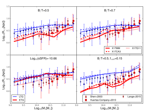
Figure 5: The $R_{1/2}$–$M_{*}$ relation, as in Fig. 2, for the X17CA3 (dashed lines) and X17G11 (dotted lines) runs, both including a treatment for dissipation during major mergers. Predictions from the X17MM model are shown as solid lines, as a reference. In the X17CA3 run, we assume that gas cooling through cold accretion has a specific angular momentum three times larger than that of the DM halo. In the X17G11 run, we assume an alternative stellar feedback scheme, based on that presented in Guo et al. (2011).

Results from the X17CA3 run are very similar to those obtained from the X17MM model for stellar masses larger than $M_{*}>10^{10.5}\;{\rm M_{\sun}}$. For lower masses, the former model predicts sizes that are offset high with respect to the X17MM run, by $\sim 0.1$ dex for LT and $\sim 0.2$ dex for ET galaxies. Therefore, the larger specific angular momentum in cold accretion significantly affects low mass galaxies. We will see in Sec. 5.4 that, in this mass range, the angular momentum of galaxies (and therefore their size) is determined at early times (where cold accretion is important), and is not significantly modified during subsequent evolution.

A different stellar feedback influences the sizes of both ET and LT galaxies, over the entire stellar mass range considered. Specifically, we find that LT galaxies in the X17G11 run have sizes that are systematically below those from the X17MM model, by about 0.2 dex. In Sec. 5.4, we will show explicitly the different evolution of galaxies in these two runs: the peak of star formation in the X17G11 run occurs earlier than in X17MM, for both LT and ET galaxies. We then expect a lower size–mass relation also for ET galaxies. This is not the case: for selections based on a $B/T$ cut, ET galaxies have, on average, sizes larger than those predicted by the X17MM run, by about $\sim 0.2$ dex. This is due to the fact that ET galaxies were subject to a similar number of mergers in the two runs, but disk instabilities occurred at earlier times in the X17G11 run. Mergers at late times increase the size of bulges. In the X17MM run, this increase can be washed out by late disk instabilities, while these are less frequent in the X17G11 run. We also find that fewer ET galaxies form mainly through disk instabilities in the X17G11 run than in the X17MM run.

4 The specific angular momentum

The correlation between sizes and masses of our model galaxies can be interpreted in relation to the angular momentum treatment. Indeed, as discussed in Sec. 2, disk radii (both of the stellar and of the gaseous component) are calculated from their specific angular momenta. Below, we use results from our model to analyze the relation between specific angular momentum and stellar mass, and its dependence on morphology and cold gas fraction.

4.1 Specific angular momentum estimate

To have a fair comparison with observational measurements, we considered several estimates for the specific angular momentum of model galaxies. In the following, we briefly describe the key quantities that we use in the discussion, and motivate our choices. The interested reader will find a more detailed description of our approach in Appendix B.

The angular momentum of the stellar component of a galaxy is the sum of the angular momenta of all stars, each proportional to the product between the distance from the center of the galaxy of the star and its velocity. Observations provide information on the projected stellar luminosity, integrated in each pixel of the galaxy image. Velocity information is inferred through spectroscopy (so these are velocities along the line of sight), either slit spectroscopy typically along the major axis of the galaxy, or integral field. In both cases, measurements are performed out to a limited galactic radius, usually corresponding to $\sim 1-2\;R_{1/2}$.

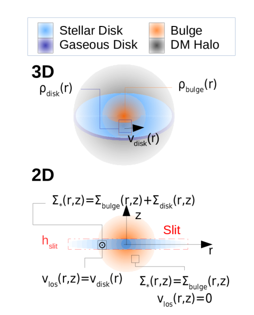
Figure 6: A schematic representation of the method adopted to calculate the 3D (top) and 2D (bottom) estimates of the angular momentum for model galaxies. See text for details.

To compute an estimate of the angular momentum of our model galaxies, we assume that the stellar mass is directly proportional to the stellar luminosity. In addition, as for the estimate of the half-mass radius, we assume an exponential profile for the surface density of the rotationally supported disk and a Jaffe profile for the bulge. Our bulge component is assumed to be dispersion supported, and therefore has always zero angular momentum by construction.

We show a schematic representation of our typical model galaxy in Fig. 6. The specific angular momentum of a galaxy can be obtained integrating the angular momentum of its components in the 3D space. We refer to this quantity as $j_{\rm tot}^{3D}$ in the following. Galaxies are, however, observed in projection. In this case, the integration is performed on the 2D plane, using the projected mass and the velocity along the line of sight, as illustrated in the bottom panel of Fig. 6. We consider two possible 2D integration methods: the first method consists in integrating the angular momentum along a slit on the major axis of the galaxy. In the second method, the integration is performed considering the entire projected galaxy, in an attempt to mimic observational measurements based on integral field spectroscopy. We refer to these two estimates as $j^{2D}_{\rm slit}$ and $j^{2D}_{\rm tot}$, respectively, both evaluated on model galaxies projected edge-on. We find that our estimates start to converge when integrating out to $\sim 2\;R_{1/2}$ (see Appendix B). In the following, when we compare our model predictions to observational measurements, we will adopt an integration radius similar to that of the observational samples considered. We also consider, for LT galaxies only, an estimate based on the empirical formula developed by Romanowsky & Fall (2012). $j^{RF}$ estimates the total specific angular momentum of disk+bulge galaxies starting from their effective radius, Sérsic index, rotational velocity at 2$R_{1/2}$ and $B/T$. Finally, we refer to the direct model output, corrected for $B/T$, as $j^{\rm SAM}_{\rm tot}=j^{\rm SAM}_{\rm disk}(1-B/T)$.

In the following, we will show model predictions as a shaded area. Specifically, we will show the area between the specific angular momentum calculated using a full 3D integration ($j^{3D}_{\rm tot}$), and that obtained using the empirical formula by Romanowsky & Fall (2012, $j^{RF}$) for LT galaxies. Typically, inclination can be easily estimated in LT galaxies, thus $j_{*}$ is integrated using de-projected quantities. In the case of ET galaxies, inclination is rather difficult to measure, and the empirical formula does not hold. For these galaxies, we will show the area between the two alternative 2D estimates: $j^{2D}_{\rm slit}$ gives an upper limit to the estimated angular momentum, while $j^{2D}_{\rm tot}$ gives a lower limit. Both these measures give a lower limit for the expected relation, as our model does not include bulge rotation.

4.2 Comparison with observations

The specific angular momentum of the disk, $j_{\rm disk}$, is much easier to estimate observationally than that of the bulge component. In particular, this is straightforward when the rotational velocity profile of the disk is inferred from the cold gas component. Selecting model galaxies with a cold gas fraction similar to that of the observational samples, we find a good agreement between the predicted median $j_{\rm disk}$–$M_{*}$ relation and recent observational estimates (see Appendix C for more details). In the following, we focus on the specific angular momenta predicted for the entire stellar component.

Fig. 7 shows the predicted $j_{*}$–$M_{*}$ relation compared with three different observational samples. Predictions from the X17MM model are shown as shaded areas, enclosing the region of the plane between $j^{3D}_{\rm tot}$ and $j^{RF}$ for LT galaxies (blue), and between $j^{2D}_{\rm slit}$ and $j^{2D}_{\rm tot}$ for ET galaxies (red). Thin solid lines of the same colors represent the scatter (16th-84th percentiles) of the distributions. We only show predictions obtained using a $B/T=0.5$ cut to distinguish between ET and LT galaxies, as different selections give qualitatively similar results. In both panels, the dashed black lines represent the theoretical expectation for the slope of the specific angular momentum versus mass relation, obtained assuming the specific angular momenta of the halo and the baryons are coupled until halo collapse ($j\propto M^{2/3}$, Mo et al., 1998). In the left panel, we show the observational measurements by Romanowsky & Fall (2012), corrected for a variable light-to-mass ratio as in Fall & Romanowsky (2013, symbols as in the legend), and those by Obreschkow & Glazebrook (2014, stars). Romanowsky & Fall (2012) collected a sample of galaxies of different morphology, with rotational velocities measured using different techniques. The specific angular momentum was estimated using a direct integration along the galaxy major axis for a sub-sample of the galaxies (out to $\sim 8\,R_{eff}$), and an empirical formula for the rest of the galaxies (for more details see Appendix B). Estimates by Obreschkow & Glazebrook (2014) are based on 16 gas-rich spiral galaxies from the THINGS survey (Leroy et al., 2008), and on HI spatially resolved velocity distribution. The integration of the specific angular momentum was carried out assuming circular annuli and out to $\sim 10\,R_{1/2}$. In this panel, we show model specific angular momenta for LT galaxies estimated out to $7\,R_{1/2}$, assuming that, at this distance, $j_{*}$ is converging to its total value. For ET galaxies, we perform an integration out to $2\,R_{1/2}$, to mimic the observational limits. In the right panel, we show the observational estimates by Cortese et al. (2016). This work is based on galaxies from the SAMI survey (dotted lines), divided according to their morphological type: Sbc (dark blue), S0/Sa-Sb (cyan), E/S0-S0 (pink) and E (red) galaxies. In this case, the specific angular momentum integration was performed in circular annuli out to $\sim 1\,R_{1/2}$. For clarity, we show the fits to the measured relations, instead of the individual data points. In this panel, the model specific angular momenta are estimated out to $1\,R_{1/2}$, to have a fair comparison with the SAMI sample. The shaded area for LT galaxies is delimited by $j^{3D}_{\rm tot}$ and $j^{2D}_{\rm tot}$, because at $1\,R_{1/2}$ there is not enough information to calculate $j^{RF}$.

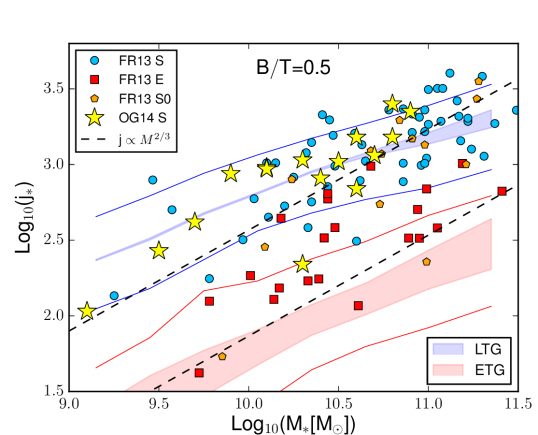
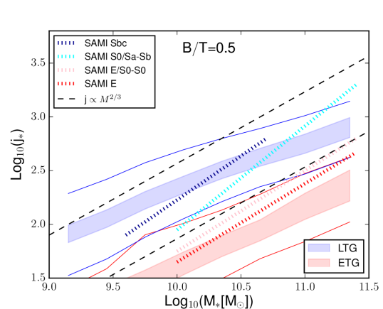
Figure 7: The $j_{*}$–$M_{*}$ relation for LT and ET galaxies from the X17MM model (blue and red shaded areas, determined as described in Sec. 4.1), compared to observational data (symbols). The thin solid lines correspond to the 16th-84th percentiles of the distributions, whereas shaded areas represent the regions covered by different estimates of $j_{*}$ (see text for details). The radial apertures used to integrate $j_{*}$ in the two panels are different, and are chosen to mimic the observational data (more details in the text). The LT/ET selection used here assumes a threshold of $B/T=0.5$. In the left panel, we show the observational measurements by Obreschkow & Glazebrook (2014, stars) and by Fall & Romanowsky (2013, other symbols), color-coded according to galaxy morphology: spirals (cyan), ellipticals (red) and lenticulars (orange). In the right panel, we show the median fits obtained for SAMI galaxies by Cortese et al. (2016, dotted lines). Different colors correspond to different galaxy morphologies, as indicated in the legend. We show as a reference the expected slope for DM halos ($j\propto M^{2/3}$) as dashed black lines.

We find that the model LT and ET galaxies follow parallel relations, with a slope similar to that measured by Fall & Romanowsky (2013) and Obreschkow & Glazebrook (2014), and only slightly lower than theoretical expectations ($j\propto M^{1/2}$ compared to the predicted $j\propto M^{2/3}$). The specific angular momentum of model galaxies is lower than that estimated from these samples, slightly in the case of LT, by $\sim 0.4$ dex for ET galaxies. Comparing model predictions to SAMI galaxies, we find that model predictions are slightly below observational measurements for ET galaxies, and exhibit a shallower relation with respect to observational data for LT galaxies. As explained in Sec. 4.1, model estimates do not account for rotating bulges that would raise the median relation found for ET model galaxies. This is shown explicitly in Appendix B, where we evaluate $j_{*}$ assuming that model bulges are all rotating following empirical relations. Using this simple assumption, the median $j_{*}$–$M_{*}$ relation is shifted up by several tenth of dex with respect to the non rotating bulge case. On the other hand, observed ET galaxies by Fall & Romanowsky (2013) were selected to have a measured rotational velocity profile. Therefore, they represent a sample biased towards fast rotators, and likely have a $j_{*}$ slightly higher than average elliptical galaxies. Slow rotators are a small but significant fraction of the observed ET galaxy population, but in our model they represent the entire ET galaxy sample. This is unrealistic, and we should interpret our model results for ET galaxies as a lower limit. SAMI ET galaxies include both fast and slow rotators, and our model predictions are closer to the median relation measured for this sample.

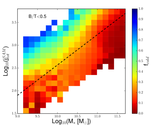
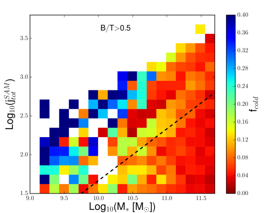
Figure 8: The $j^{\rm SAM}_{\rm tot}$–$M_{*}$ relation for X17MM galaxies, color coded by the median cold gas fraction ($f_{\rm cold}$) in each pixel. The left panel corresponds to LT galaxies ($B/T<0.5$), the right to ET galaxies ($B/T>0.5$). A different color scale has been used in the two panels. Model $j^{\rm SAM}_{\rm tot}$ values shown here correspond to the model output disk specific angular momentum, weighted for the bulge contribution. We also show, as dashed black lines, the theoretical expectation for the slope of the relation ($j\propto M^{2/3}$).

In the case of LT galaxies, Fall & Romanowsky (2013) and Obreschkow & Glazebrook (2014) used samples that include classical, gas-rich, spiral galaxies. Our selection of model LT galaxies based on $B/T$ includes both classical spirals and lenticulars with subdominant bulges. Therefore, compared to our model, observational samples appear biased towards gas-rich galaxies. In our model, the cold gas fraction $f_{\rm cold}=M_{\rm cold}/(M_{\rm cold}+M_{*})$ strongly correlates with $j_{*}$, as shown in Fig. 8. In this figure, we show the distribution of model galaxies in the $j^{\rm SAM}_{\rm tot}$–$M_{*}$ plane, color-coded by the median $f_{\rm cold}$ in each pixel. We choose $j^{\rm SAM}_{\rm tot}$ as a $j_{*}$ estimator, in order to have a comparable quantity for LT and ET galaxies. This quantity is not directly comparable to the shaded areas shown in Fig. 7, but results do not change qualitatively. Left and right panels show the distributions of LT and ET galaxies, respectively. As above, we have used a simple $B/T=0.5$ cut to separate different galaxy types, and we have used a different color scale for the two panels, to highlight the trends as a function of the gas fractions. Gas rich galaxies have larger specific angular momenta than gas poor galaxies of the same stellar mass. The relation with stellar mass is somewhat steeper for gas rich galaxies, and the slope in better agreement with theoretical expectations ($j\propto M^{2/3}$). If we select LT galaxies with $f_{\rm cold}>0.3$ and $B/T<0.5$, the predicted median $j_{*}$–$M_{*}$ relation shifts up by $\sim 0.3$ dex. The correlation between $j_{*}$ and $f_{\rm cold}$ is strong for $B/T<0.4$. For $B/T$ values in the range $0.4<B/T<0.7$, the correlation is not as clear, and there are gas-poor galaxies with quite high values of $j_{*}$. For $B/T>0.7$, the correlation is again strong. This effect is evident in the right panel of Fig. 8, where the relation for ET galaxies exhibits a dependence on the cold gas fraction less pronounced than for LT galaxies, in particular at intermediate to high stellar masses. This behavior can be ascribed to the presence of galaxies dominated by bulges formed mainly through disk instabilities. These galaxies retain, on average, less gas than galaxies with bulges formed mainly through mergers, at fixed stellar mass and $j_{*}$. As we will show in detail in Sec. 5.2, disk instabilities can form massive bulges only through a series of subsequent star formation and disk instability episodes. Recurring star formation depletes the cold gas available in the disk, washing out the correlation between the cold gas content and the specific angular momentum.

Estimates of the angular momentum of LT galaxies based on SAMI (blue dotted lines in the right panel of Fig. 7) appear to follow a steeper relation than our model predictions, and than previous observational estimates. As noted in Cortese et al. (2016) their best fits are still consistent with the expected ${2/3}$ slope. In addition, their measurements are based on apertures smaller ($\sim 1R_{1/2}$) than those used in Fall & Romanowsky (2013). For a sub-sample of their galaxies, they were able to measure the specific angular momentum out to $\sim 2R_{1/2}$, obtaining a higher normalization and a better agreement with Fall & Romanowsky (2013). When changing the aperture radius, we find that the normalization of the $j_{*}$–stellar mass relation changes, but the slope is unaffected, as can be noted comparing the two panels (see also Appendix B).

4.3 Specific angular momentum in X17CA3 and X17G11

We show in Fig. 9 the $j_{*}$–$M_{*}$ relation for two modified versions of our model: one assuming a larger angular momentum for gas accreted during the rapid cooling regime (X17CA3, hatched areas), and one with a stellar feedback scheme based on that used in Guo et al. (2011) (X17G11, areas with circles). Galaxies are classified as LT and ET using a $B/T=0.5$ cut. We show also results from the X17MM model as a reference (shaded areas). The areas are determined as described in Sec. 4.1. The model stellar specific angular momenta are obtained integrating $j_{*}$ out to $2\;R_{1/2}$, as a compromise between convergence and limited radii typically available in observational studies.

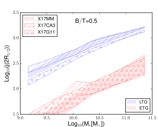
Figure 9: The $j_{*}$–$M_{*}$ relation for LT and ET galaxies (blue and red colors), evaluated for galaxies from the X17MM run (shaded areas), the X17CA3 run (hatched areas), and the X17G11 run (areas with circles). The areas are determined as described in Sec. 4.1. All models include dissipation during major mergers. LT and ET galaxies were selected using the $B/T=0.5$ threshold.

The separation between LT and ET galaxies is evident in all the three models considered here. The X17CA3 run returns predictions that are almost identical to the X17MM run for massive galaxies ($M_{*}>10^{10.5}\;{\rm M_{\sun}}$), while at low masses the former model predicts higher values of $j_{*}$ with respect to our reference run. Therefore, low mass galaxies are more affected by the higher angular momentum acquired during cold accretion, while for high mass galaxies this accretion mode is less important in determining the final value of $j_{*}$. We reached similar conclusions when analyzing the $R_{1/2}$–$M_{*}$ relation.

LT galaxies in the X17G11 run have a lower median $j_{*}$ with respect to X17MM, over the entire mass range considered. We interpret this result as due to the different stellar feedback scheme, which causes most of the stars to form earlier than in our reference model. As the angular momentum is lower at earlier cosmic epochs, this leads to a lower normalization of the $j_{*}$–$M_{*}$ relation. For ET galaxies, X17G11 returns predictions consistent with those from X17MM, for $M_{*}>10^{10.5}\;{\rm M_{\sun}}$. At lower masses, the angular momentum predicted by the modified feedback model is systematically larger than that obtained using our fiducial X17MM run, by $\sim 0.2$ dex. In Sec. 3.3, we have seen that ET galaxies in the X17G11 run have, on average, larger sizes that their counterparts of the X17MM run. The specific angular momentum integration is influenced by the larger size of the bulges, which translates into larger values of $j_{*}$.

5 Evolution of angular momentum and dependence on other galactic properties

In the previous section, we have demonstrated that the scatter in the $j_{*}$–$M_{*}$ relation correlates both with galaxy morphology and with gas fraction. Below, we analyze in detail the evolutionary processes driving these correlations.

5.1 Bulge formation channels and size–mass relation

In this Section, we briefly describe the different origin of LT and ET galaxies in our model. This subject has been discussed, for previous versions of our model, in several studies (Fontanot et al., 2011; De Lucia et al., 2011; De Lucia et al., 2012; Wilman et al., 2013). Since the basic statistics are qualitatively the same, we will focus our analysis on those aspects that are useful to interpret the original results discussed in this paper.

Our model bulge can grow through mergers and disk instabilities. We have evaluated the relative importance of these two channels for galaxies in the X17MM model, in bins of stellar mass and $B/T$. We have excluded satellite galaxies from this analysis but most results discussed below remain qualitatively the same when including them, except when otherwise stated.

Table 2 lists the fraction of central galaxies that have experienced, from $z=1$ to the present day: (i) no relevant disk instability event (no DI, with relevant we mean an episode characterized by $\delta M_{*}/M_{*,disk}>0.1$, where $\delta M_{*}$ is the fraction of stellar disk that is transferred to the bulge to restore stability); (ii) no major merger (no MM, $M_{sat}/M_{cen}>0.3$); (iii) no minor merger (no mM) with a mass ratio $0.1<M_{sat}/M_{cen}<0.3$). The table shows that a significant fraction of galaxies did not experience any minor merger since $z=1$. This suggests that minor mergers are not the main channel for the formation of bulges in these galaxies. Major mergers are more likely to occur in galaxies with $B/T>0.7$, or in low mass galaxies with $B/T>0.5$. Disk instabilities are very frequent in the intermediate $B/T$ bin, in particular at intermediate and high stellar masses.

Table 2: Fraction of central galaxies that did not experience a relevant disk instability episode (no DI), a major merger (no MM), or a minor merger (no mM), from $z=1$ to the present day. Different rows correspond to different stellar mass bins. A further selection is made according to galaxy morphology: $B/T<0.5$ (first column), $0.5<B/T<0.7$ (second column) and $B/T>0.7$ (third column).

		$B/T<0.5$			$0.5<B/T<0.7$			$B/T>0.7$
$M_{*}\;[{\rm M_{\sun}}]\in$	no DI	no MM	no mM	no DI	no MM	no mM	no DI	no MM	no mM
$[10^{9.6};\;10^{10.2}]$	0.97	0.99	0.88	0.76	0.30	0.85	0.98	0.03	0.81
$[10^{10.2};\;10^{10.8}]$	0.94	0.99	0.92	0.12	0.90	0.97	0.90	0.09	0.90
$[10^{10.8};\;10^{11.5}]$	0.95	1.	0.82	0.29	0.97	0.88	0.96	0.08	0.82

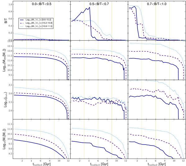
Figure 10: Median evolution as a function of look-back time of some galactic properties, for central galaxies. From top to bottom: B/T, $M_{200}$, $j_{\rm halo}$ and $M_{*}$. Model galaxies have been selected according to their stellar mass at redshift 0: $M_{*}\in[10^{9.6-10.2}]$ (solid blue lines), $[10^{10.2},10^{10.8}]$ (dashed violet lines) and $[10^{10.8},10^{11.5}]\;{\rm M_{\sun}}$ (dotted light blue lines). Different columns correspond to different values of $B/T$. Vertical yellow lines are for reference.

Fig. 10 shows the median evolution of some selected properties as a function of lookback time. In this figure, central galaxies are divided according to their final stellar mass, as in the table. Different line-styles correspond to different stellar mass bins as indicated in the legend, while different columns correspond to different $B/T$ bins. The figure shows that the bulges of low mass galaxies are formed mainly through major mergers, which translates into an abrupt increase of the $B/T$ value following the merger events. Low-mass LT and ET galaxies reside in halos of similar mass, with halos of ET galaxies only slightly less massive than those hosting LT galaxies ($M_{200}^{LT}\sim 10^{11.4}\;{\rm M_{\sun}}$ and $M_{200}^{ET}\sim 10^{11.1}\;{\rm M_{\sun}}$ at redshift 0). On average, halos hosting ET galaxies in this stellar mass bin formed later than those hosting LT galaxies: the former accrete half of their final mass 9 Gyrs ago, the latter 10 Gyrs ago. These small differences suggest that ET and LT galaxies in this mass bin belong to the same ‘halo population’, and that the differentiation occurs because of the occurrence of major mergers for ET galaxies.

For the intermediate and large stellar mass galaxies ($M_{*}\in[10^{10.2};\,10^{11.5}]\,M_{\sun}$), we find more significant differences between the parent halos of different types. For galaxies with $B/T<0.7$, the median parent halo masses at $z=0$ are $M_{200}^{int}\sim 10^{11.7}{\rm M_{\sun}}$ and $M_{200}^{high}\sim 10^{12.3}{\rm M_{\sun}}$ for intermediate and high stellar mass bin, respectively. For $B/T>0.7$, the numbers become $M_{200}^{int}\sim 10^{12}{\rm M_{\sun}}$ and $M_{200}^{high}\sim 10^{12.8}{\rm M_{\sun}}$. Therefore, the $B/T=0.7$ threshold separates two different galaxy populations: one formed in relatively small halos and the other one formed in more massive halos, that likely experience more merger events. Intermediate and massive galaxies with $B/T>0.7$ form most of their bulge mass through mergers: the fraction of galaxies that did not experience any merger in this $B/T$ range varies between 3 and 7 per cent, depending on the stellar mass bin. Intermediate and massive galaxies with $B/T<0.7$, in contrast, form their bulge mainly through disk instability. In this case, the probability of building a relevant bulge depends on the specific history of the galaxy and of its halo. The main difference between galaxies with $B/T<0.5$ and those with $0.5<B/T<0.7$ is in the specific angular momentum of their halos, $j_{\rm h}$. Galaxies with a more prominent bulge have a smaller $j_{\rm h}$ for most of their history. The small $j_{\rm h}$ is transferred to the cold gas disk through cooling, and then to the stellar disk through star formation. Stellar disks in galaxies with $0.5<B/T<0.7$ are thus smaller than those associated with $B/T<0.5$ galaxies. This affects the stability of the disk: at fixed stellar mass, halos with smaller $j_{\rm h}$ have a higher probability to undergo a disk instability episode. We further discuss the origin and evolution of disk instabilities in the next section.

5.2 Disk instability in central and satellite galaxies

In the previous sections, we have found that the contribution of disk instability to bulge growth is significant for galaxies with $0.5<B/T<0.7$ and $M_{*}\in[10^{10.2};\;10^{10.8}]\;{\rm M_{\sun}}$. Fig. 10 and Table 2 show that the contribution of this bulge formation channel is important also for massive central galaxies with intermediate morphology ($0.5<B/T<0.7$). As we have seen earlier, the relevance of the disk instability channel reflects in the size–mass relation (because DI bulges are smaller than merger bulges). The effect is more important at intermediate masses because in this mass bin galaxies with $0.5<B/T<0.7$ are more numerous than those with $B/T>0.7$.

In Sec. 3.2, we have shown that, for intermediate mass ET galaxies, centrals selected using a $B/T=0.5$ threshold have on average a smaller half-mass radius than the overall population of ET galaxies. This is in part due to the fact that bulges of central galaxies have a slightly larger contribution from disk instability with respect to those of the overall population ($\sim 50\%$ in centrals and $\sim 46\%$ in all galaxies). Furthermore, bulges and disks in central galaxies that underwent disk instabilities have smaller sizes (by $\sim 0.7$ dex) than those formed in satellites of the same mass and $B/T$. Below, we discuss the origin of these differences in more detail.

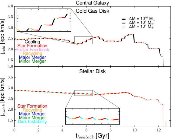
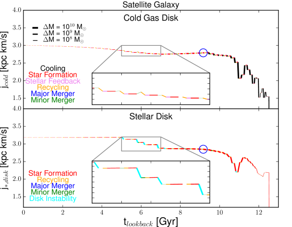
Figure 11: Evolution of the specific angular momentum of two representative galaxies with $10^{10.2}<M_{*}<10^{10.8}\;{\rm M_{\sun}}$ and $0.5<B/T<0.7$. The left panels show the evolution of a central galaxy, while the right panels are for a satellite. The top panels show the evolution of the specific angular momentum of the cold gas disk, while the bottom panels show that of the stellar disk. The colored segments represent variations of the specific angular momentum, and are color coded according to the physical process causing them (see legend). The thickness of each segment increases with the absolute magnitude of the mass variation resulting from each process. The zoomed-in regions highlight recursive disk instability events.

Fig. 11 shows the evolution as a function of lookback time of the specific angular momentum of the gaseous disks (top panels) and of the stellar disks (bottom panels) for a central (left panels) and a satellite galaxy (right panels). These test galaxies have been selected within $10^{10.2}<M_{*}<10^{10.8}\;{\rm M_{\sun}}$ and $0.5<B/T<0.7$, and are representative of the whole sample. Each segment shows a variation of specific angular momentum due to a specific physical process (different colors correspond to different processes, as indicated in the legend). Let us focus first on the evolution of the central galaxy (left panels). At early times ($t_{\rm lookback}>10\;{\rm Gyr}$), the specific angular momentum of the gaseous disk grows due to cooling (black lines in the top panel). The specific angular momentum of the cold gas is unaffected by star formation and stellar feedback (red and magenta lines), and only slightly decreases due to recycling (orange lines). The angular momentum of the cold gas follows the variation of the angular momentum of the parent halo: it starts decreasing after $t_{\rm lookback}\sim 10\;{\rm Gyr}$, increases again at $t_{\rm lookback}\sim 7\;{\rm Gyr}$, and then decreases again until $t_{\rm lookback}\sim 5\;{\rm Gyr}$. The stellar disk acquires the angular momentum of the cold gas through star formation (bottom left panel). When $j_{\rm*,disk}$ decreases, the disk contracts until it eventually becomes unstable. As described in Sec. 2.2.3, during disk instability events, part of the disk mass is transferred to the bulge to restore the stability. Since we assume angular momentum is conserved, this increases the specific angular momentum (and size) of the disk. These events are shown as cyan lines in the bottom left panel of Fig. 11. During subsequent star formation episodes (see the zoom-in panel), the stellar disk mass increases again, the cold gas decreases, and so does the specific angular momentum. This triggers a new disk instability episode. The size of the galaxy therefore oscillates slightly, due to a series of consecutive disk instability events.

In the case of the satellite galaxy (right panels), the early evolution of the gaseous and stellar disks is similar to that of the central galaxy. After accretion (the last time the galaxy is a central - marked as a blue circle in the figure), the angular momentum of the cold gaseous disk cannot be affected by cooling, which is suppressed. The stellar disk follows the evolution of the cold gas due to star formation. After accretion, star formation still occurs, but at increasingly lower rates (thinner red segments), because gas is consumed and not replenished via cooling. Also in this case, the instability criterion is eventually met, and the satellite undergoes a disk instability episode. Similarly to the case of the central galaxy examined above, the satellite enters a recursive cycle of star formation and disk instability episodes. In this case, the stellar disk specific angular momentum (and thus scale radius) remains almost constant due to star formation, but the newly formed stars trigger a new instability event. This leads to an increase of the specific angular momentum of the stellar disk. In satellites, $j_{\rm cold}$ is not lowered by cooling, and keeps growing due to recycling from the stellar disk. This translates into higher $j_{*}$ also for stars formed from the cold gas disk. This sequence of events stops only when the star formation becomes negligible, because the cold gas is nearly exhausted.

The two examples analyzed are representative of the total population: statistically, disk instabilities affect only slightly the size of central galaxies, while they generally lead to a slight increase of the size of satellite galaxies.

5.3 Angular momentum and cold gas

We have shown earlier that there is a strong dependence of the specific angular momentum–mass relation on the cold gas fraction of model galaxies. In this section, we investigate in detail the origin of this dependence, by analyzing the evolution of gas-rich and gas-poor central galaxies. Also in this case we focus on central galaxies, but we find consistent results for satellites. We show the median evolution of some galaxy properties in Fig. 12, as we did in Fig. 10. We divide our model galaxies in the same stellar mass bins at z=0: low ($M_{*}\in[10^{9.6}-10^{10.2}]\;{\rm M_{\sun}}$, solid), intermediate ($M_{*}\in[10^{10.2}-10^{10.8}]\;{\rm M_{\sun}}$, dashed), and high ($M_{*}\in[10^{10.8}-10^{11.5}]\;{\rm M_{\sun}}$, dotted lines). Results are qualitatively similar for different values of $B/T$, so we average galaxies of different morphological types. For completeness, we show the evolution for different bins in B/T in Appendix D. For each mass sample considered, we have selected galaxies belonging to the extremes of the $f_{\rm cold}$ distribution: i.e. we consider galaxies with $f_{\rm cold}$ smaller than the 16^th percentile of the distribution as gas-poor, and those with $f_{\rm cold}$ larger than the 84^th percentile as gas-rich. Lines are color-coded according to the stellar mass bin and the cold gas fraction, as indicated in the legend.

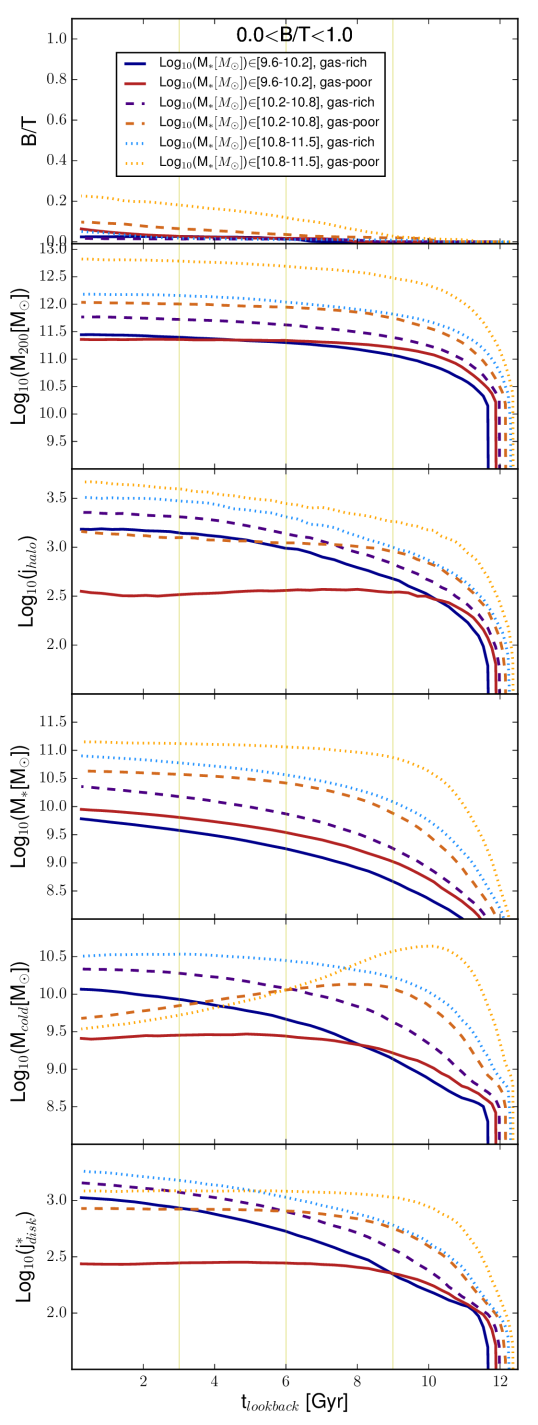
Figure 12: Median evolution as a function of lookback time of several galactic properties of model central galaxies in bins of stellar mass (different line-styles), and cold gas fraction (different colors). From top to bottom: B/T, $M_{200}$, $j_{\rm halo}$, $M_{*}$, $M_{\rm cold}$ and $j_{\rm*,disk}$. Galaxies have been selected according to their stellar mass at redshift 0; gas poor/rich galaxies are selected as those below/above the 16th/84th percentile of the distribution.

For all mass bins considered, gas-poor galaxies are hosted by halos that form earlier than those of gas-rich galaxies. The halos hosting gas-poor galaxies grow rapidly in mass, and acquire most of their angular momentum during this phase of rapid accretion. The accretion history of halos hosting gas-poor galaxies translates into large amounts of cold gas in these galaxies at early times, which triggers significant early star formation. Most of the stellar mass of gas-poor galaxies is formed between 9 and 11 Gyrs ago. At this time, the specific angular momentum of the cold gas is relatively low, like that of the parent dark matter haloes. In contrast, gas-rich galaxies are hosted by halos that formed more recently than those hosting gas-poor galaxies. These halos accrete their mass more gradually, and their mass increases down to very recent times. As a consequence, star formation occurs over a longer interval of time, and the stellar disk can acquire the higher specific angular momentum of the halo at late times.

5.4 Dependence on physical prescriptions

In this section, we study the origin of the different size–mass and specific angular momentum–mass relations for the fiducial model X17MM and for its variants X17CA3 and X17G11. In Fig. 13 and 14, we show the evolution of the total stellar mass and of the stellar disk specific angular momentum for ET (red) and LT (blue) galaxies, divided using a $B/T=0.7$ cut. Predictions from different models are shown using different line styles (X17MM with solid, X17CA3 with dashed, and X17G11 with dotted lines).

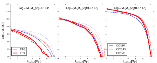
Figure 13: Median evolution of the total stellar mass as a function of lookback time , for galaxies in different stellar mass bins (different panels). Galaxies are classified as LT (blue) and ET (red) using a threshold at $B/T=0.7$. Different linestyles correspond to different models: solid for the X17MM model, dashed for X17CA3, and dotted for X17G11.

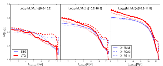
Figure 14: As in Fig. 13, but this time showing the median evolution of the stellar disk specific angular momentum as a function of lookback time.

In the X17CA3 run, the gas cooling in the rapid mode regime has an angular momentum three times larger than in the X17MM run. As we have discussed earlier, this leads to slightly larger sizes and angular momenta for low-mass galaxies ($M<10^{10.2}\;{\rm M_{\sun}}$). When considering the evolution of X17CA3 galaxies (dashed lines in the figures), we see that their specific angular momentum is higher than in the X17MM model during the first 2-3 Gyrs, as expected. This, however, does not imply a higher star formation rate, because a larger $j_{\rm cold}$ translates into a larger disk radius and, as a consequence, a lower gas surface density. As a result, the stellar mass of galaxies in the X17CA3 run evolves as in X17MM, although the specific angular momentum of the stellar disk is much higher at early epochs ($j_{*}$ follows $j_{\rm cold}$ through star formation). After 2-3 Gyrs, cold accretion is no longer the dominating accretion mode, and the specific angular momentum of the cold gas converges to approximately the same values found in the X17MM run.

For the X17G11 run, we found a lower final specific angular momentum for LT galaxies and, as a consequence, a lower normalization of the size–mass relation. In Fig. 13, we find that X17G11 galaxies form the bulk of their stars at earlier times compared to their counter-parts in the X17MM run, for all the mass and morphology bins considered. The feedback scheme adopted in the X17G11 run allows ejected gas to be reaccreted earlier than in X17MM, resulting in larger amounts of gas cooling onto the model galaxies in the first 1-2 Gyrs. This translates into significant early star formation. After the initial peak, star formation gradually decreases, while in the fiducial model it remains almost constant down to the present day. This is because in the X17MM run, ejected gas is reaccreted more gradually. Therefore, most of the stars in the disk of X17G11 galaxies form from gas with lower specific angular momentum than in the X17MM run, explaining the systematic offsets we find for sizes and angular momenta of model LT galaxies. In Sec. 3.3, we have shown that ET galaxies in the X17G11 run have, on average, larger sizes than those of the same mass in the X17MM run. This is contrary to what one would expect considering the evolution of the specific angular momentum just discussed. For ET galaxies, however, one has to consider also the different merger and disk instability histories in the two runs. We find that in the X17G11 run, the star formation peak occurs earlier than for X17MM, and this tends to decrease the occurrence of later disk instability episodes. As a consequence, more bulges in the X17G11 run are formed mainly during mergers with respect to X17MM, which leads to an average bulge size in the X17G11 run larger than in X17MM. When evaluating the specific angular momentum of ET galaxies in the X17G11 model, the larger bulge sizes affect the integration, because, at fixed mass, the bulge profile is flatter. This enhances the importance of rotational velocity at large radii in the calculation of $j_{*}$. The rotational velocity increases with radius, and the integrated final specific angular momentum is thus higher than in the X17MM model.

6 Discussion and conclusions

In this work, we have analyzed the structural and dynamical properties of galaxies in the framework of a state-of-the-art semi-analytic model. In particular, we have used the latest version of the GAlaxy Evolution and Assembly (GAEA Hirschmann et al., 2016) model. This includes a sophisticated treatment for the non-instantaneous recycling of gas, metals, and energy (De Lucia et al., 2014), and a new stellar feedback scheme partly based on results from hydrodynamical simulations (Hirschmann et al., 2016). The model we have used also includes a treatment for the atomic to molecular gas transition based on the Blitz & Rosolowsky (2006) empirical relation, and a molecular hydrogen based star formation law (Xie et al., 2017). Furthermore, our model includes prescriptions to follow the angular momentum exchanges among galactic components, and evaluates disk sizes from specific angular momenta, as in Guo et al. (2011). In the following subsections, we discuss our results focusing on: (i) comparison between model predictions and the observed size–mass and angular momentum–mass relations; (ii) relevance of disk instability and limits of our modeling approach; and (iii) dependence on different physical prescriptions.

6.1 Size and specific angular momentum

Our galaxy formation model traces explicitly the exchanges of specific angular momentum between different galactic components, and this information is used to evaluate the disk scale radius. Therefore, the size–mass and the angular momentum–mass relation of model disk galaxies are strictly related to each other. For bulge dominated galaxies, whose sizes are estimated using energy conservation arguments and for which the contribution from disk instability can be important, the correlation between size and angular momentum is less trivial, also due to the approximations necessary to estimate the latter quantity (see Appendix B).

Previous studies focused on the size–mass relation at relatively high masses ($M_{*}>10^{10}\;{\rm M_{\sun}}$), and highlighted the necessity of a specific treatment for gas dissipation during mergers to obtain realistic bulge sizes (Shankar et al., 2013; Tonini et al., 2016). In our study, we have extended the comparison with observational results down to stellar masses of $\sim 10^{9}\;{\rm M_{\sun}}$. For late type galaxies, our predicted size–mass relation is in fairly good agreement with recent observational estimates. In agreement with previous studies, we find that dissipation during mergers is necessary to correctly reproduce the size of early type galaxies, especially at low stellar masses ($M_{*}<10^{10}\;{\rm M_{\sun}}$). In our model, we find that dissipation must be limited to major mergers, otherwise the predicted bulge sizes are too small compared to observational measurements. This assumption is reasonable since the prescriptions we have used are based on binary merger simulations, with relatively large mass ratios. These simulations show that the effect of dissipation is more relevant in major mergers between spiral galaxies, and influences only slightly minor mergers between spiral galaxies (see Porter et al., 2014, and their Table 1, for a summary of their results). Our results are also in agreement with those by Shankar et al. (2013), who applied the same treatment for dissipation, only during major mergers, to the semi-analytic model by Guo et al. (2011).

In the framework of our model, the specific criteria used to select late and early type galaxies affect significantly the predicted size–mass relation, which appears to be in contrast with observational findings. Specifically, we find that using a selection based on the bulge-to-total mass ratio (B/T) leads to two well separated relations for late and early type galaxies, and to a reasonable agreement with observational measurements. In contrast, when selecting galaxies on the basis of their specific star formation rate (sSFR), model early type galaxies are offset high with respect to data, and their size–mass relation does not differ significantly from that obtained for active model galaxies. If we consider only central galaxies, the size–mass relation predicted adopting a sSFR selection for early type galaxies is in agreement with results based on a $B/T$ selection. The treatment of satellites in our model is rather simple: after the accretion, the hot gas reservoir is instantaneously stripped and assigned to the central halo, suppressing cold gas refueling through cooling. This treatment suppresses the star formation in satellite galaxies, but does not affect their morphology and size. Our model does not include a treatment for physical processes such as tidal interactions, which can effectively remove material from the galaxy outskirts. The introduction of these processes could reduce the sizes of satellite galaxies and even affect their morphology.

Our model predictions for the specific angular momentum versus mass relation agree fairly well with observational measurements in terms of slope, but are offset low with respect to data both for early and late type galaxies. For bulge dominated galaxies, this offset can be partially explained by the fact that we assume our model bulges do not rotate. For late type galaxies this could be explained, at least in part, by selection biases towards gas-rich galaxies. In fact, we find a relatively strong correlation between the specific angular momentum and the gas fraction. This correlation is a by-product of halo and galaxy evolution: gas poor galaxies form most of their stars at high redshift where the angular momentum of the parent halo is low, while gas rich galaxies tend to form stars over a longer time-scale allowing larger values of angular momentum. We found a similar correlation in Zoldan et al. (2017), where we have shown that the neutral atomic hydrogen content of our model galaxies is correlated with the halo spin parameter. These results highlight how the halo evolution influences at the same time the specific angular momentum and cold gas evolution. Future surveys, with a higher completeness and better controlled selection, will provide us with more robust estimates of the specific angular momentum versus mass relations. These results will allow us to identify the origin of the discrepancies discussed above.

The success of our model in reproducing the specific angular momenta of galaxies is rather impressive, given the intrinsic limitations of the semi-analytic approach in treating spatially resolved quantities. The same subject has been addressed in the framework of only a few other models. Lagos et al. (2015) analyzed the misalignment between the specific angular momenta of the cold gas, of the stellar disks, and of the DM halo. In their work, they used a modelling for angular momentum exchanges similar to ours, but added a specific post-processing treatment for spin flips during galaxy mergers/accretions. They did not compare, however, the amplitude of the predicted specific angular momenta with observational estimates. Stevens et al. (2016) used a more sophisticated modelling for the evolution of the disk specific angular momentum. Specifically, they divided the galactic disk in annuli of different specific angular momentum, and evolved them according to physical processes applied to the individual annuli. Their predicted $j_{{\rm*,disk}}$–$M_{*}$ relation for spiral galaxies agrees well with observational measurements by Fall & Romanowsky (2013) and Obreschkow & Glazebrook (2014). They found that the normalization of the relation is strongly affected by disk instabilities: the specific angular momentum decreases when disk instability is turned off. Our disk instability treatment appears to have a similar effect on $j_{{\rm*,disk}}$, but its influence on the evolution of LT galaxies is overall less important. Stevens et al. (2016) did not model the specific angular momenta of galaxies with $B/T>0.3$ so that their results cannot be directly compared to ours.

Our comparison with observational data has been limited to the local Universe. We plan to extend this comparison to higher redshift in future work. We note, however, that the strong correlation between the specific angular momentum of the stellar disk with that of the DM halo suggests an evolution similar to that observed, at least for late type galaxies.

6.2 Disk instability and bulge size

In our model, central bulge-dominated galaxies have unrealistically small sizes in the stellar mass range $10^{10}-10^{10.8}\;M_{\sun}$. This is not the case when considering the entire early-type galaxy population (i.e. including satellite galaxies), and is due to different contributions and sizes of bulges that form predominantly through disk instability or mergers. Specifically, we find that most of the intermediate bulges ($0.5<B/T<0.7$) form mainly through disk instabilities, while the largest ones ($B/T>0.7$) form mainly through (major) mergers. The sizes of our model bulges formed through mergers are in nice agreement with observational estimates (with a relatively small under-estimation with respect to observational data at large stellar masses), while disk instabilities produce systematically smaller bulges, especially for central galaxies. We find that disk instability events are typically associated with haloes that suffer, at some point of their life-time, a decrease of specific angular momentum. As the hot gas is assumed to have the same specific angular momentum as the dark matter halo, cooling transfers this loss of specific angular momentum to the cold gas disk, and star formation transfers it to the stellar disk. This eventually triggers recursive events of disk instability. In our satellite galaxies, disk instabilities tend to result in a net increase of stellar disk sizes, because cooling is suppressed after accretion. For central galaxies, the size of the stellar disk component oscillates slightly but is not significantly different from the value it had before the instability episodes.

The unrealistic sizes obtained for bulges formed through disk instability highlight the need to revise the prescriptions adopted for this particular physical process. The instability criterion we currently use is based on old two-dimensional N-body simulations of a purely stellar disk in a rigid halo (Efstathiou et al., 1982). Although widely adopted in the semi-analytic framework, this criterion is not consistent with results from more recent N-body simulations (Athanassoula, 2008, and references therein). At present, however, no alternative prescription is available.

The bulge size estimation during disk instabilities should also be revised. Secular processes are believed to give origin to thick, disk-like, rotating ‘pseudo-bulges’. These differ from classical, merger originated bulges in their dynamical properties and in their stellar population (see Kormendy & Kennicutt, 2004, for a review). The scale length of classical and pseudo-bulges are, however, comparable (Fisher & Drory, 2008; Gadotti, 2009), contrary to predictions from our model. Recently, Tonini et al. (2016) considered an explicit division between classical and pseudo bulges in their semi-analytic model, assuming disk-like structural properties for pseudo-bulges. In their model, pseudo-bulges have masses similar to those of classical bulges, but are concentrated in the $M_{B}\in[10^{10},10^{11}]\;{\rm M_{\sun}}$ range. In general, their pseudo-bulges have small half-mass radii (up to $5$ kpc), while classical bulges are larger (up to $20$ kpc). In our model, disk instability bulges are much smaller than 1 kpc. Assuming that stars in disk instability bulges are distributed according to an exponential profile, we obtain half-mass radii larger than those represented in Fig. 3 of about $\sim 0.5$ dex. A consistent treatment of a two components bulge would allow the formation of larger bulges, because the larger radii of disk instability bulges would enter the energy equation during mergers. Furthermore, a rotating pseudo-bulge would allow for an explicit treatment of fast and slow rotators, and model results could be consistently compared with results from recent integral field spectroscopic surveys, as ATLAS^3D and SAMI. Similar studies have been carried out in the framework of semi-analytic models, but without an explicit analysis of the specific angular momentum of fast and slow rotators (see e.g. Khochfar et al., 2011). We postpone a self-consistent implementation of a two-bulge model to a future work.

6.3 Dependence on physical modeling: stellar feedback and cooling

Our analysis confirms that the dynamical properties of galaxies depend strongly on the galaxy star formation and assembly history. We have tested the relative importance of specific prescriptions regulating the baryon cycle. Specifically, we have considered an alternative stellar feedback scheme, and the influence of a higher specific angular momentum for gas cooling in rapid mode.

In the alternative feedback scheme considered, the ejected gas is re-accreted earlier than in our fiducial model. This causes the bulk of star formation to occur earlier than in our reference model. Since the halo angular momentum is generally lower at higher redshift, the alternative scheme translates into a lower specific angular momentum. Several studies based on hydrodynamic simulations have highlighted that strong stellar feedback at early times leads to high final specific angular momentum of the stellar disk (Übler et al., 2014; Hirschmann et al., 2013). In these simulations, the gas ejected through stellar winds is accelerated and re-accreted with angular momentum higher than it had when it was ejected. Our model does not include such a sophisticated treatment for ejected gas. Simply, the reaccreted gas has the same specific angular momentum of the dark matter halo at the time of gas re-accretion. This means that the re-accreted gas has indeed an angular momentum typically larger than at the time of ejection. Our results confirm the fundamental role of stellar feedback in determining the dynamical properties of galaxies, by regulating the time when most of the stars are formed (and therefore most of the angular momentum is acquired).

We have also analyzed the influence of a higher specific angular momentum for gas cooled in the rapid cooling regime. This was motivated by results from recent hydrodynamic simulations (Stewart et al., 2011; Pichon et al., 2011; Danovich et al., 2015), that have highlighted that this gas can have angular momentum from 2 to 4 times larger than that of the parent dark matter halo halo. Including this modification in our model, the star formation history of model galaxies is not significantly affected. We find that small galaxies are those mostly affected, with slightly larger sizes and angular momenta than those in our reference model. Therefore, we expect this physical process to be important at higher redshift, where a larger fraction of the population is dominated by the cold accretion mode.

6.4 Summary

We have shown that results from our GAlaxy Evolution and Assembly (GAEA) model, modified to include a treatment for gas dissipation during major mergers, are in quite nice agreement with the observed size–mass and specific angular momentum–mass relation observed in the local Universe. The main conclusions of our work can be summarized as follows:

• The predicted size–mass and specific angular momentum–mass relations are in fairly good agreement with observational measurements when late and early type galaxies are selected using a cut in bulge-to-total (B/T) stellar mass. A late/early type selection based on the specific star formation rate (sSFR) would instead include, in our model, too many quenched disky satellite galaxies, leading to a too high normalization of the size–mass relation for early type galaxies.

• The sizes of our model bulges are strongly affected by their dominant formation channel. Bulges formed mainly through disk instabilities have unrealistically small sizes. This affects, in particular, central galaxies with $0.5<B/T<0.7$ and $M_{*}\in[10^{10};\;10^{10.8}]\;M_{\sun}$. We have discussed how an explicit treatment for a two-bulge component could lead to a better agreement with data.

• The stellar specific angular momentum of a galaxy is strongly correlated with its cold gas fraction. This correlation originates naturally from the galaxy accretion history: in gas-poor galaxies today, most of the stars are formed at early times when the halo angular momentum is low. In contrast, gas-rich galaxies form their stars over a more extended time-scale, which allows larger angular momentum to be incorporated in the stellar component of galaxies.

• The adopted stellar feedback scheme can affect significantly the galaxy star formation history, and therefore the predicted angular momenta and sizes of model galaxies. A shift to higher (lower) redshift of the peak of star formation leads to a lower (higher) normalization of the angular momentum/size–mass relation for late time galaxies. For early-type galaxies, the shift might be less important or even go in the opposite direction, in our model, due to a different contribution from the disk instability channel.

• A different initial specific angular momentum of cold gas accreted through rapid cooling regime influences the sized and angular momenum of small galaxies today, and is expected to have an important impact at higher redshift where a larger fraction of the galaxy population is dominated by this accretion mode.

Appendix A Mass and velocity profiles

We assume that the stellar and gaseous disks are described by exponential surface density profiles:

$$\Sigma_{\rm disk}(r)=\Sigma_{0}e^{-\frac{r}{R_{\rm disk}}}$$ (8)

where $R_{\rm disk}$ is the scale radius, and $\Sigma_{0}=M_{\rm*,disk}/(2\pi R_{\rm disk}^{2})$ the central surface density. For the bulge, we assume a stellar distribution that follows a Jaffe profile (Jaffe, 1983):

$$\rho(r)=\frac{M_{B}}{4\pi R_{B}^{3}}\left(\frac{r}{R_{B}}\right)^{-2}\left(1+\frac{r}{R_{B}}\right)^{-2}$$ (9)

where $R_{B}$ is the scale radius, and $M_{B}$ is the mass of the bulge. The half-mass radii ($R_{1/2}$) of model galaxies are obtained projecting the stellar mass profiles in Eq.s 8 and 9 assuming galaxies are seen face on, and calculating the radius that encloses half of the projected mass.

To estimate the galaxy specific angular momentum, we assume that the bulge is dispersion supported ($v_{\rm bulge}(\vec{r})=0$), and that the stellar disk is symmetric and supported by rotation:

$$v_{\rm rot}^{\rm disk}(r)=\sqrt{\frac{GM(<r)}{r}},$$ (10)

where $G$ is the gravitational constant, and $M(<r)$ is the total mass enclosed within $r$. It includes the stars in the disk and in the bulge, the gas in the disk, and the corresponding fraction of the parent dark matter halo. For the latter component, we assume a Navarro-Frenk-White profile (Navarro et al., 1996):

$$\rho(r)=\frac{\rho_{0}}{\frac{r}{R_{\rm DM}}\left(1+\frac{r}{R_{\rm DM}}\right)^{2}},$$ (11)

where $\rho_{0}$ and $R_{\rm DM}$ are a density parameter and the scale radius of the halo. Both can be estimated using the concentration parameter of the halo, which we calculate using the correlation between $M_{200}$ and concentration published in Neto et al. (2007). This relation has a large scatter, but we checked that our results are not significantly affected by this using the extremes of the distribution, instead of the median. The virial radius is directly proportional to the scale radius: $R_{200}=cR_{\rm DM}$, while the density parameter $\rho_{0}$ can be obtained integrating Eq. 11 to $R_{200}$ and forcing it to be equal to $M_{200}$. The latter quantity is measured directly from the simulations for all haloes hosting central galaxies, while for satellites it corresponds to the particle mass times the number of bound particles in the parent subhalo. $R_{200}$ is calculated from $M_{200}$, given the redshift of the halo.

Appendix B Specific angular momentum estimates

For a comparison with observational measurements of the specific angular momentum, we consider different estimates for our model galaxies. We refer to the cartoons in Fig. 6, to help the reader in visualizing the description below.

The first estimate we consider is based on a three dimensional (3D) model of the galaxy (see the top panel of Fig. 6). Using the 3D mass and velocity distributions for each galaxy, we calculate the specific angular momentum within the radius $R$, by integrating the velocity and mass profiles over all radii $r<R$. The specific angular momentum of the disk, obtained integrating on the plane of the disk, is:

$$j_{\rm disk}^{3D}(R)=\frac{\int_{0}^{R}r\;v_{\rm rot}^{\rm disk}(r)\;\Sigma_{\rm disk}(r)\;r\;dr}{\int_{0}^{R}\Sigma_{\rm disk}(r)\;r\;dr}$$ (12)

If we include the bulge, for which we assume $v_{\rm bulge}(r)=0$, we obtain:

$$j_{\rm tot}^{3D}(R)=\frac{\int_{0}^{R}r\;v_{\rm rot}^{\rm disk}(r)\;\Sigma_{\rm disk}(r)r\;dr}{\int_{0}^{R}\Sigma_{\rm disk}(r)r\;dr+\int_{0}^{R}\rho_{\rm bulge}(r)4\pi r^{2}dr}$$ (13)

where the integration for the bulge is carried out in 3D space.

In observations, the 3D information is not available: the galaxy is projected on the sky (2D), with a random inclination, and the velocity information is typically available only along the line of sight (l.o.s.). In addition, it is difficult to separate the contributions from the bulge and the disk. We mimic this situation assuming all model galaxies are edge-on (see the bottom panel of Fig. 6). In the 2D projection, we adopt a cartesian coordinate system centered at the galactic center, and aligned with the disk plane ($r$ coordinate) and the disk rotation axis ($z$ coordinate). In this way, the l.o.s. velocity measured along the disk, at a projected distance $r$ from the center, is exactly the rotational velocity at the 3D distance $r^{3D}=r$: $v_{\rm los}(r)=v_{\rm rot}^{\rm disk}(r)$. We project the stellar profiles of the stellar disk and of the bulge on the edge-on plane, and sum them into a single stellar component: $\Sigma_{*}(r,z)=\Sigma_{\rm disk}^{\rm edge-on}(r,z)+\Sigma_{\rm bulge}(r,z)$. We also assume $h_{\rm disk}=R_{\rm disk}/7.3$ (Kregel et al., 2002), and:

$$v_{\rm los}(r,z)=\begin{cases}v_{\rm rot}^{\rm disk}(r)&{\rm if\;}z<h_{\rm disk}\\ 0&{\rm if\;}z>h_{\rm disk}\end{cases}$$

In this way, the bulge fraction contained in a cylinder of height $h_{\rm disk}$ cannot be disentangled from the projected disk and, in the integration, it is assumed to rotate with the disk. We assume there is no rotation outside the cylinder. The specific angular momentum calculated along a slit of the same height of the disk $h_{\rm slit}=h_{\rm disk}$ is:

$$j_{\rm slit}^{2D}(R)=\frac{\int_{0}^{R}\int_{0}^{h_{\rm slit}}r\;v_{\rm los}(r,z)\;\Sigma_{*}(r,z)\;dr\;dz}{\int_{0}^{R}\int_{0}^{h_{\rm slit}}\Sigma_{*}(r,z)\;dr\;dz}$$ (14)

Including also the bulge component outside the slit:

$$j_{\rm tot}^{2D}(R)=\frac{\int_{0}^{R}\int_{0}^{R}r\;v_{\rm los}(r,z)\;\Sigma_{*}(r,z)\;dr\;dz}{\int_{0}^{R}\int_{0}^{R}\Sigma_{*}(r,z)\;dr\;dz}$$ (15)

These estimates mimic the integrations performed for observed projected galaxies, with $j_{\rm tot}^{2D}$ similar to an integration on circular or elliptical concentric annuli, and $j_{\rm slit}^{2D}$ similar to an integration along the major axis. In the case of LT galaxies, a precise estimate of the galaxy inclination is usually possible, and the integration is performed using de-projected quantities. In the case of ET galaxies or spheroids, this is more difficult, as the precise measure of their rotational velocity. In this case a rough estimate of $j_{*}$ is given by the projected integration.

Romanowsky & Fall (2012) found that the total specific angular momentum is well approximated, after de-projection for inclination, by an empirical formula that depends on the effective radius, the velocity measured at two effective radii, and a factor $k_{n}$ that depends on the Sérsic index. In the case of a disk+bulge galaxy, they sum the contributions from the disk and the bulge, weighting them for the corresponding light (mass) fraction, $D/T$ and $B/T$:

$$j_{D+B}=k_{n_{D}}v_{\rm disk}(2R_{D}^{e})R_{D}^{e}\frac{D}{T}+k_{n_{B}}v_{\rm bulge}(2R_{B}^{e})R_{B}^{e}\frac{B}{T}$$ (16)

In the above equation, $n_{x}$ and $R_{x}^{e}$ are the Sérsic index and the effective radius of the disk ($x=D$), or of the bulge ($x=B$). The disk velocity $v_{\rm disk}(2R_{D}^{e})$ is measured from the ionized gas of the disk, while the bulge rotational velocity $v_{\rm bulge}(2R_{B}^{e})$ is estimated from its relation with the ellipticity $\epsilon$ and central velocity dispersion $\sigma_{0}$, through:

$$v_{\rm bulge}=\left(\frac{v}{\sigma}\right)^{*}\sigma_{0}\left(\frac{\epsilon}{1-\epsilon}\right)^{1/2}$$ (17)

$(v/\sigma)^{*}\sim 0.7$ is a parameter describing the relative dynamical importance of rotation and pressure, and a value equal to one corresponds to that of an oblate isotropic system viewed edge-on (Kormendy & Illingworth, 1982). The value of $0.7$ was chosen following the work by Romanowsky & Fall (2012).

We assume all model galaxies are composed of a disk+bulge, with a disk Sérsic index $n_{D}=1$ ($k_{1}=1.19$), $v_{\rm bulge}=0$, and $\epsilon=0$. Thus the second part of Eq. 16 is always zero and:

$$j^{RF}=k_{1}\;v_{\rm rot}^{\rm disk}(2R_{D}^{e})\;R_{D}^{e}\frac{D}{T}$$ (18)

The assumption of perfectly spherical, dispersion dominated bulges is very strong. We evaluate its impact by assuming, alternatively, that all bulges have a Sérsic index $n_{B}=4$ ($k_{4}=2.29$), an ellipticity $\epsilon=0.2$ (this is the median ellipticity of the elliptical/lenticular SDSS galaxies as found in Hao et al., 2006), and a velocity dispersion evaluated using the virial theorem: $\sigma_{0}=\sqrt{G(M_{B}+\delta M_{\rm disk})/(2R_{B})}$. In the last equation, $\delta M_{\rm disk}$ is the fraction of the disk that influences the bulge dynamics, which we assume to be the disk inside $R_{B}$ (higher values do not affect significantly model results). Eq. 16 then can be written as:

$$j^{RF}_{\epsilon=0.2}=k_{1}v_{\rm rot}^{\rm disk}(2R_{D}^{e})R_{D}^{e}\frac{D}{T}+k_{4}0.35\sqrt{\frac{G(M_{B}+\delta M_{\rm disk})}{2R_{B}}}R_{B}^{e}\frac{B}{T}$$ (19)

The different estimates computed can also be compared to the standard output of our model ($j_{\rm disk}^{\rm SAM}$), weighted for the bulge contribution: $j_{\rm tot}^{\rm SAM}=j_{\rm disk}^{\rm SAM}(1-B/T)$.

Fig. 15 shows the median $j^{2D}_{\rm slit}$–$M_{*}$ relation evaluated at 1, 2 and 3 $R_{1/2}$. The difference between 2$R_{1/2}$ and 3$R_{1/2}$ is much smaller than that between 2$R_{1/2}$ and 1$R_{1/2}$. In the paper, we show $j_{*}$ integrated out to a radius similar to that of the observational samples considered. When observations extrapolate to the total $j_{*}$, we use $j_{*}$ integrated out to $7\,R_{1/2}$, assuming its value has converged to the total value. In the comparison between different runs of the model, we use the specific angular momentum corresponding to 2$R_{1/2}$, a distance that provides a good compromise between convergence and typical observational limits.

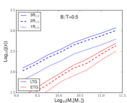
Figure 15: The $j_{\rm slit}^{2D}$–$M_{*}$ relation for LT and ET galaxies (blue and red), selected by their morphology ($B/T=0.5$), from the X17MM model. The $j_{\rm slit}^{2D}(r)$ is evaluated considering projected profiles at different radii: $r=1,2,3\;R_{1/2}$.

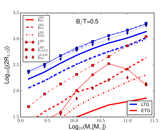
Figure 16: The median $j$–$M_{*}$ relation for LT and ET galaxies (blue and red) selected by their morphology ($B/T=0.5$). All $j_{*}$ estimates are evaluated at $2R_{1/2}$. Different lines and symbols represent different estimates for the specific angular momentum, as detailed in the text and as indicated in the legend.

Fig. 16 shows the median $j$–$M_{*}$ relation predicted for LT (blue) and ET (red) galaxies from the X17MM model. We only consider a selection assuming a $B/T=0.5$ cut here, but we have verified that results are qualitatively similar for alternative selections. Different line styles correspond to the different estimates introduced earlier, as indicated in the legend. All relations obtained for LT galaxies, based on different estimates of $j_{*}$, are above the ET relations. The estimates $j^{RF}$ and $j^{RF}_{\epsilon=0.2}$ give almost identical relations for LT galaxies, and correspond to the highest normalization of the $j_{*}$–$M_{*}$ relation for these galaxies. This is expected, because the influence of bulges in eq.s 18 and 19 for galaxies with $B/T<0.5$ is negligible. The relation assuming the direct model output, $j^{\rm SAM}_{\rm tot}$, is only slightly below that based on the empirical formula proposed by Romanowsky & Fall (2012). The relation based on the 3D estimate, $j^{3D}_{\rm tot}$, is parallel to these but is offset low by $\sim 0.2$ dex. Both the 2D estimates $j_{\rm slit}^{2D}$ and $j_{\rm tot}^{2D}$ lie on the same relation, shifted 0.2 dex below that based on the 3D estimate. This is not surprising, because LT galaxies have a small bulge, and a large fraction of it is contained in the slit. The difference with respect to the 3D estimate is due to the projection of the disk mass: most of the disk mass, residing at the center, has a lower velocity than in the de-projected case. We expect that for inclinations lower than edge-on this relation moves up towards the 3D relation. This argument is valid only for LT galaxies for which the bulges, whose projected distribution is spherical and does not depend on inclination, do not dominate the central stellar mass distribution.

While different estimates of $j_{*}$ for LT galaxies correspond to parallel relations with relatively small shifts, estimates obtained for ET galaxies cover a much larger region of the $j_{*}$–$M_{*}$ plane. As for LT galaxies, the highest normalizations are obtained for the empirical estimates by Romanowsky & Fall (2012), $j^{RF}_{\epsilon=0.2}$ and $j^{RF}$. The $j_{*}$–$M_{*}$ relation based on the estimate that includes rotation in bulges, $j^{RF}_{\epsilon=0.2}$, lies very close to the relation obtained for LT galaxies employing the 2D estimates, with a slightly steeper slope. Romanowsky & Fall (2012) derived the formulae for $j^{RF}$ and $j^{RF}_{\epsilon=0.2}$ to describe disk+bulge galaxies. They analyzed $j_{*}$ of a small sub-sample of elliptical galaxies using alternative measurements, finding little convergence. Nevertheless, they used the formula to estimate $j_{*}$ for their total sample. Therefore, the relation we show for ET galaxies should be intended as a rough estimate of our expectations for a realistic population of rotating bulges, with the caveat that the validity of the formula used has not been assessed for $B/T>0.5$. As expected, the $j^{RF}_{\epsilon=0.2}$ estimate is larger than that obtained assuming $\epsilon=0$ ($j^{RF}$). The latter does not include a bulge velocity component, and the calculation depends only on the disk size and its velocity. The dependence on the disk size is important, because measuring the disk radius in a bulge dominated galaxy is not easy. In fact, using the effective radius of the galaxy in the $j^{RF}$ estimations, instead of the disk effective radius, lowers the relation at intermediate masses to the same position of the relation based on the $j^{2D}_{\rm tot}$ estimate (for $M_{*}<10^{10.7}\;{\rm M_{\sun}}$). The relation obtained considering the direct model output for ET galaxies, $j^{\rm SAM}_{\rm tot}$, is close to that obtained using $j^{RF}$. The specific angular momentum increases with increasing stellar mass up to $M_{*}\sim 10^{10.7}\;{\rm M_{\sun}}$; for larger stellar masses, the median value of $j^{\rm SAM}_{\rm tot}$ first flattens and then decreases. The relation assuming the 2D circular estimate, $j_{\rm tot}^{2D}$, is parallel to that obtained using $j^{2D}_{\rm slit}$, but is shifted up by 0.3-0.4 dex. We tested the influence of the slit height $h_{\rm slit}$ on the predicted $j_{*}$–$M_{*}$ relation, finding that a smaller $h_{\rm slit}$ would shift $j_{\rm slit}^{2D}$ upwards, and $j_{\rm tot}^{2D}$ downwards. For a slit with height of $\sim 0.1h_{\rm slit}$, the shift of the relation using $j_{\rm slit}^{2D}$ is of 0.1 dex, while that of the relation based on $j_{\rm tot}^{2D}$ is of 0.2 dex - a modest effect. The relation corresponding to the 3D estimate, $j^{3D}_{\rm tot}$, is well below the other relations, because it does not mix bulge stars within the rotating disk, as happens in the projected estimates.

Appendix C Comparison of the disk specific angular momentum to observations

We compare the specific angular momenta of our model disks to the observational data by Posti et al. (2018), based on the SPARC galaxy sample (Lelli et al., 2016). These galaxies have a well studied rotational velocity profile, estimated from the HI. The specific angular momentum profile is integrated out to large radii (around $\sim 5\,R_{\rm disk}$ most of the velocity profiles are found to converge). Since the sample is composed of gas rich spirals, we estimate the HI fraction in both observations and model galaxies, and estimate the influence of different selections on the final $j_{\rm disk}$–$M_{*}$ median relation.

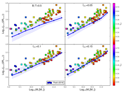
Figure 17: The $j_{\rm disk}$–$M_{*}$ relation predicted for LT galaxies (blue solid lines) from the X17MM run. The $j_{\rm disk}$ value is integrated out to 2 disk scale radii. Different panels show different LT selections. Shaded areas show the region between the 16th and 84th percentiles of the distribution. Symbols correspond to the observational measurements by Posti et al. (2018), colour-coded according to their $f_{\rm HI}$.

Fig. 17 shows the median $j_{\rm disk}$–$M_{*}$ relation (solid blue line) we obtain for galaxies selected using $B/T<0.5$ (top left panel), and an additional threshold constraint for the HI fraction $f_{\rm HI}=M_{\rm HI}/(M_{*}+M_{\rm HI})$ (other panels, as indicated in the captions). The model median relation corresponds to the 3D specific angular momentum of the stellar disks, evaluated out to 2 scale radii. Squares represent the observational data by Posti et al. (2018), color-coded according to their $f_{\rm HI}$. Observational data show a clear correlation between HI gas fraction and $j_{\rm disk}$, with HI-rich galaxies having a higher specific angular momentum than gas-poor galaxies at fixed stellar mass. Furthermore, the HI gas fraction correlates with stellar mass, with higher stellar masses corresponding to lower average HI fractions. The model predicted median relation shifts upwards, particularly at the high mass end, when imposing a threshold on the cold gas fraction. When using a cut that is similar to that of the observational sample, model predictions agree relatively well with data.

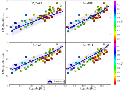
Figure 18: As in Fig. 17, but integrating the model specific angular momentum out to 6 disk scale radii.

We also integrated $j_{\rm disk}$ out to 6 disk scale radii, assuming this length as sufficient for convergence. Results are shown in figure 18. The median relation is shifted upwards by 0.2 dex for all the selections. This does not affect significantly our conclusions.

Appendix D Morphology and cold gas content

Fig. 19 is similar to Fig. 12, but considering a further binning of model galaxies according to their $B/T$ (different columns).

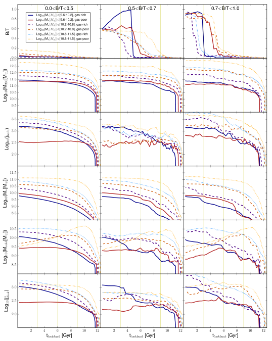
Figure 19: Median evolution as a function of lookback time of several galactic properties. From top to bottom: B/T, $M_{200}$, $j_{\rm halo}$, $M_{*}$, $M_{\rm cold}$, $SFR$, and stellar disk specific angular momentum. Model galaxies have been selected according to their stellar mass at redshift 0, as indicated in the legend. A further binning is made as a function of the cold gas fraction $f_{\rm cold}$, with gas-rich (indigo, purple and pink) and gas-poor galaxies (chocolate, orange and gold) selected as those above or below the upper or lower 16th percentile of the distributions, respectively. Different colors are used for galaxies of different stellar mass, as indicated in the legend.

In Sec. 5.3, we have shown that the higher specific angular momentum of gas-rich galaxies, with respect to gas poor ones, is due to a larger contribution from recent star formation. This, in turn, is due to the different accretion histories of their hosting haloes. When considering galaxies divided in bins of $B/T$, we find an evolution similar to that found for the entire population. The figure shows that gas-poor ET galaxies, at redshift zero, contain less gas than LT galaxies. In addition, the bulges of gas-poor galaxies form on average 2-3 Gyrs earlier than those of gas-rich galaxies. This is a selection effect, due to the fact that galaxies with higher star formation rates can regrow a disk more efficiently. As star formation correlates with the gas content, the star formation rates are larger in gas rich galaxies, that can quickly regrow a significant disk component. A certain $B/T$ threshold selects gas-poor ET galaxies that formed their bulge earlier than gas-rich galaxies. This is because the latter, in the meanwhile, have already regrown their disks.

References

- Abadi et al. (2003) Abadi M. G., Navarro J. F., Steinmetz M., Eke V. R., 2003, ApJ, 591, 499
- Andredakis & Sanders (1994) Andredakis Y. C., Sanders R. H., 1994, MNRAS, 267, 283
- Athanassoula (2008) Athanassoula E., 2008, MNRAS, 390, L69
- Bacon et al. (2001) Bacon R., et al., 2001, MNRAS, 326, 23
- Barnes & Efstathiou (1987) Barnes J., Efstathiou G., 1987, ApJ, 319, 575
- Barnes & Hernquist (1991) Barnes J. E., Hernquist L. E., 1991, ApJ, 370, L65
- Benson (2012) Benson A. J., 2012, New Astron., 17, 175
- Benson & Devereux (2010) Benson A. J., Devereux N., 2010, MNRAS, 402, 2321
- Blitz & Rosolowsky (2006) Blitz L., Rosolowsky E., 2006, ApJ, 650, 933
- Boylan-Kolchin et al. (2009) Boylan-Kolchin M., Springel V., White S. D. M., Jenkins A., Lemson G., 2009, MNRAS, 398, 1150
- Bryant et al. (2015) Bryant J. J., et al., 2015, MNRAS, 447, 2857
- Bundy et al. (2015) Bundy K., et al., 2015, ApJ, 798, 7
- Cappellari et al. (2011) Cappellari M., et al., 2011, MNRAS, 413, 813
- Carollo et al. (2001) Carollo C. M., Stiavelli M., de Zeeuw P. T., Seigar M., Dejonghe H., 2001, ApJ, 546, 216
- Ceverino et al. (2015) Ceverino D., Dekel A., Tweed D., Primack J., 2015, MNRAS, 447, 3291
- Cole et al. (2000) Cole S., Lacey C. G., Baugh C. M., Frenk C. S., 2000, MNRAS, 319, 168
- Cortese et al. (2016) Cortese L., et al., 2016, MNRAS, 463, 170
- Covington et al. (2011) Covington M. D., Primack J. R., Porter L. A., Croton D. J., Somerville R. S., Dekel A., 2011, MNRAS, 415, 3135
- Cox et al. (2008) Cox T. J., Jonsson P., Somerville R. S., Primack J. R., Dekel A., 2008, MNRAS, 384, 386
- Croton et al. (2006) Croton D. J., et al., 2006, MNRAS, 365, 11
- Dalcanton et al. (1997) Dalcanton J. J., Spergel D. N., Summers F. J., 1997, ApJ, 482, 659
- Danovich et al. (2015) Danovich M., Dekel A., Hahn O., Ceverino D., Primack J., 2015, MNRAS, 449, 2087
- Davis & Bureau (2016) Davis T. A., Bureau M., 2016, MNRAS, 457, 272
- Davis et al. (2011) Davis T. A., et al., 2011, MNRAS, 417, 882
- De Lucia & Blaizot (2007) De Lucia G., Blaizot J., 2007, MNRAS, 375, 2
- De Lucia et al. (2010) De Lucia G., Boylan-Kolchin M., Benson A. J., Fontanot F., Monaco P., 2010, MNRAS, 406, 1533
- De Lucia et al. (2011) De Lucia G., Fontanot F., Wilman D., Monaco P., 2011, MNRAS, 414, 1439
- De Lucia et al. (2012) De Lucia G., Fontanot F., Wilman D., 2012, MNRAS, 419, 1324
- De Lucia et al. (2014) De Lucia G., Tornatore L., Frenk C. S., Helmi A., Navarro J. F., White S. D. M., 2014, MNRAS, 445, 970
- DeFelippis et al. (2017) DeFelippis D., Genel S., Bryan G. L., Fall S. M., 2017, ApJ, 841, 16
- Driver et al. (2011) Driver S. P., et al., 2011, MNRAS, 413, 971
- Drory & Fisher (2007) Drory N., Fisher D. B., 2007, ApJ, 664, 640
- Efstathiou et al. (1982) Efstathiou G., Lake G., Negroponte J., 1982, MNRAS, 199, 1069
- Eke et al. (2000) Eke V., Efstathiou G., Wright L., 2000, MNRAS, 315, L18
- Elmegreen et al. (2008) Elmegreen B. G., Bournaud F., Elmegreen D. M., 2008, ApJ, 688, 67
- Fall (1983) Fall S. M., 1983, in Athanassoula E., ed., IAU Symposium Vol. 100, Internal Kinematics and Dynamics of Galaxies. pp 391–398
- Fall & Efstathiou (1980) Fall S. M., Efstathiou G., 1980, MNRAS, 193, 189
- Fall & Romanowsky (2013) Fall S. M., Romanowsky A. J., 2013, ApJ, 769, L26
- Fisher & Drory (2008) Fisher D. B., Drory N., 2008, AJ, 136, 773
- Fontanot et al. (2011) Fontanot F., De Lucia G., Wilman D., Monaco P., 2011, MNRAS, 416, 409
- Fontanot et al. (2017) Fontanot F., Hirschmann M., De Lucia G., 2017, ApJ, 842, L14
- Gadotti (2009) Gadotti D. A., 2009, MNRAS, 393, 1531
- Genel et al. (2015) Genel S., Fall S. M., Hernquist L., Vogelsberger M., Snyder G. F., Rodriguez-Gomez V., Sijacki D., Springel V., 2015, ApJ, 804, L40
- Governato et al. (2004) Governato F., et al., 2004, ApJ, 607, 688
- Governato et al. (2010) Governato F., et al., 2010, Nature, 463, 203
- Grand et al. (2017) Grand R. J. J., et al., 2017, MNRAS, 467, 179
- Grogin et al. (2011) Grogin N. A., et al., 2011, ApJS, 197, 35
- Guedes et al. (2011) Guedes J., Callegari S., Madau P., Mayer L., 2011, ApJ, 742, 76
- Guo et al. (2011) Guo Q., et al., 2011, MNRAS, 413, 101
- Guo et al. (2013) Guo Q., White S., Angulo R. E., Henriques B., Lemson G., Boylan-Kolchin M., Thomas P., Short C., 2013, MNRAS, 428, 1351
- Hao et al. (2006) Hao C. N., Mao S., Deng Z. G., Xia X. Y., Wu H., 2006, MNRAS, 370, 1339
- Hirschmann et al. (2013) Hirschmann M., et al., 2013, MNRAS, 436, 2929
- Hirschmann et al. (2016) Hirschmann M., De Lucia G., Fontanot F., 2016, MNRAS, 461, 1760
- Hopkins et al. (2009) Hopkins P. F., Hernquist L., Cox T. J., Keres D., Wuyts S., 2009, ApJ, 691, 1424
- Hopkins et al. (2010) Hopkins P. F., et al., 2010, ApJ, 715, 202
- Hopkins et al. (2014) Hopkins P. F., Kereš D., Oñorbe J., Faucher-Giguère C.-A., Quataert E., Murray N., Bullock J. S., 2014, MNRAS, 445, 581
- Huertas-Company et al. (2013) Huertas-Company M., Shankar F., Mei S., Bernardi M., Aguerri J. A. L., Meert A., Vikram V., 2013, ApJ, 779, 29
- Ichikawa et al. (2012) Ichikawa T., Kajisawa M., Akhlaghi M., 2012, MNRAS, 422, 1014
- Jaffe (1983) Jaffe W., 1983, MNRAS, 202, 995
- Katz (1992) Katz N., 1992, ApJ, 391, 502
- Kennicutt et al. (2007) Kennicutt Jr. R. C., et al., 2007, ApJ, 671, 333
- Khochfar et al. (2011) Khochfar S., et al., 2011, MNRAS, 417, 845
- Kormendy & Illingworth (1982) Kormendy J., Illingworth G., 1982, ApJ, 256, 460
- Kormendy & Kennicutt (2004) Kormendy J., Kennicutt Jr. R. C., 2004, ARA&A, 42, 603
- Kregel et al. (2002) Kregel M., van der Kruit P. C., de Grijs R., 2002, MNRAS, 334, 646
- Lagos et al. (2009) Lagos C. D. P., Padilla N. D., Cora S. A., 2009, MNRAS, 395, 625
- Lagos et al. (2015) Lagos C. d. P., Padilla N. D., Davis T. A., Lacey C. G., Baugh C. M., Gonzalez-Perez V., Zwaan M. A., Contreras S., 2015, MNRAS, 448, 1271
- Lagos et al. (2018) Lagos C. d. P., et al., 2018, MNRAS, 473, 4956
- Lange et al. (2015) Lange R., et al., 2015, MNRAS, 447, 2603
- Lange et al. (2016) Lange R., et al., 2016, MNRAS, 462, 1470
- Lelli et al. (2016) Lelli F., McGaugh S. S., Schombert J. M., 2016, AJ, 152, 157
- Leroy et al. (2008) Leroy A. K., Walter F., Brinks E., Bigiel F., de Blok W. J. G., Madore B., Thornley M. D., 2008, AJ, 136, 2782
- MacArthur et al. (2003) MacArthur L. A., Courteau S., Holtzman J. A., 2003, ApJ, 582, 689
- Marinacci et al. (2014) Marinacci F., Pakmor R., Springel V., 2014, MNRAS, 437, 1750
- Mo et al. (1998) Mo H. J., Mao S., White S. D. M., 1998, MNRAS, 295, 319
- Murante et al. (2015) Murante G., Monaco P., Borgani S., Tornatore L., Dolag K., Goz D., 2015, MNRAS, 447, 178
- Muratov et al. (2015) Muratov A. L., Kereš D., Faucher-Giguère C.-A., Hopkins P. F., Quataert E., Murray N., 2015, MNRAS, 454, 2691
- Navarro & Steinmetz (2000) Navarro J. F., Steinmetz M., 2000, ApJ, 538, 477
- Navarro et al. (1996) Navarro J. F., Frenk C. S., White S. D. M., 1996, ApJ, 462, 563
- Neto et al. (2007) Neto A. F., et al., 2007, MNRAS, 381, 1450
- Obreschkow & Glazebrook (2014) Obreschkow D., Glazebrook K., 2014, ApJ, 784, 26
- Peebles (1969) Peebles P. J. E., 1969, ApJ, 155, 393
- Peletier & Balcells (1996) Peletier R. F., Balcells M., 1996, AJ, 111, 2238
- Pichon et al. (2011) Pichon C., Pogosyan D., Kimm T., Slyz A., Devriendt J., Dubois Y., 2011, MNRAS, 418, 2493
- Planck Collaboration et al. (2014) Planck Collaboration et al., 2014, A&A, 571, A16
- Porter et al. (2014) Porter L. A., Somerville R. S., Primack J. R., Johansson P. H., 2014, MNRAS, 444, 942
- Posti et al. (2018) Posti L., Fraternali F., Di Teodoro E. M., Pezzulli G., 2018, A&A, 612, L6
- Romanowsky & Fall (2012) Romanowsky A. J., Fall S. M., 2012, ApJS, 203, 17
- Sánchez et al. (2012) Sánchez S. F., et al., 2012, A&A, 538, A8
- Serra et al. (2014) Serra P., et al., 2014, MNRAS, 444, 3388
- Shankar et al. (2013) Shankar F., Marulli F., Bernardi M., Mei S., Meert A., Vikram V., 2013, MNRAS, 428, 109
- Sharma & Steinmetz (2005) Sharma S., Steinmetz M., 2005, ApJ, 628, 21
- Shen et al. (2003) Shen S., Mo H. J., White S. D. M., Blanton M. R., Kauffmann G., Voges W., Brinkmann J., Csabai I., 2003, MNRAS, 343, 978
- Sokołowska et al. (2017) Sokołowska A., Capelo P. R., Fall S. M., Mayer L., Shen S., Bonoli S., 2017, ApJ, 835, 289
- Somerville et al. (2001) Somerville R. S., Primack J. R., Faber S. M., 2001, MNRAS, 320, 504
- Spergel et al. (2003) Spergel D. N., et al., 2003, ApJS, 148, 175
- Springel et al. (2001) Springel V., White S. D. M., Tormen G., Kauffmann G., 2001, MNRAS, 328, 726
- Springel et al. (2005) Springel V., et al., 2005, Nature, 435, 629
- Steinmetz & Navarro (1999) Steinmetz M., Navarro J. F., 1999, ApJ, 513, 555
- Stevens et al. (2016) Stevens A. R. H., Croton D. J., Mutch S. J., 2016, MNRAS, 461, 859
- Stewart et al. (2011) Stewart K. R., Kaufmann T., Bullock J. S., Barton E. J., Maller A. H., Diemand J., Wadsley J., 2011, ApJ, 735, L1
- Teklu et al. (2015) Teklu A. F., Remus R.-S., Dolag K., Beck A. M., Burkert A., Schmidt A. S., Schulze F., Steinborn L. K., 2015, ApJ, 812, 29
- Tonini et al. (2016) Tonini C., Mutch S. J., Croton D. J., Wyithe J. S. B., 2016, MNRAS, 459, 4109
- Übler et al. (2014) Übler H., Naab T., Oser L., Aumer M., Sales L. V., White S. D. M., 2014, MNRAS, 443, 2092
- Walter et al. (2008) Walter F., Brinks E., de Blok W. J. G., Bigiel F., Kennicutt Jr. R. C., Thornley M. D., Leroy A., 2008, AJ, 136, 2563
- Wang et al. (2008) Wang J., De Lucia G., Kitzbichler M. G., White S. D. M., 2008, MNRAS, 384, 1301
- Weil et al. (1998) Weil M. L., Eke V. R., Efstathiou G., 1998, MNRAS, 300, 773
- Weinmann et al. (2009) Weinmann S. M., Kauffmann G., van den Bosch F. C., Pasquali A., McIntosh D. H., Mo H., Yang X., Guo Y., 2009, MNRAS, 394, 1213
- White (1984) White S. D. M., 1984, ApJ, 286, 38
- White & Frenk (1991) White S. D. M., Frenk C. S., 1991, ApJ, 379, 52
- Wilman et al. (2013) Wilman D. J., Fontanot F., De Lucia G., Erwin P., Monaco P., 2013, MNRAS, 433, 2986
- Wong & Blitz (2002) Wong T., Blitz L., 2002, ApJ, 569, 157
- Xie et al. (2017) Xie L., De Lucia G., Hirschmann M., Fontanot F., Zoldan A., 2017, MNRAS, 469, 968
- York et al. (2000) York D. G., et al., 2000, AJ, 120, 1579
- Zavala et al. (2016) Zavala J., et al., 2016, MNRAS, 460, 4466
- Zoldan et al. (2017) Zoldan A., De Lucia G., Xie L., Fontanot F., Hirschmann M., 2017, MNRAS, 465, 2236
- de Jong (1996) de Jong R. S., 1996, A&A, 313, 45
- van den Bosch et al. (2002) van den Bosch F. C., Abel T., Croft R. A. C., Hernquist L., White S. D. M., 2002, ApJ, 576, 21
- van den Bosch et al. (2003) van den Bosch F. C., Abel T., Hernquist L., 2003, MNRAS, 346, 177
- van der Wel et al. (2014) van der Wel A., et al., 2014, ApJ, 788, 28