Predicting the Neutral Hydrogen Content of Galaxies From Optical Data Using Machine Learning

Abstract

We develop a machine learning-based framework to predict the Hi  content of galaxies using more straightforwardly observable quantities such as optical photometry and environmental parameters. We train the algorithm on $z=0-2$ outputs from the Mufasa cosmological hydrodynamic simulation, which includes star formation, feedback, and a heuristic model to quench massive galaxies that yields a reasonable match to a range of survey data including Hi. We employ a variety of machine learning methods (regressors), and quantify their performance using the root mean square error (rmse) and the Pearson correlation coefficient (r). Considering SDSS photometry, 3^rd nearest neighbor environment and line of sight peculiar velocities as features, we obtain r $>0.8$ accuracy of the Hi-richness prediction, corresponding to rmse$<0.3$. Adding near-IR photometry to the features yields some improvement to the prediction. Compared to all the regressors, random forest shows the best performance, with r $>0.9$ at $z=0$, followed by a Deep Neural Network with r $>0.85$. All regressors exhibit a declining performance with increasing redshift, which limits the utility of this approach to $z\la 1$, and they tend to somewhat over-predict the Hi content of low-Hi galaxies which might be due to Eddington bias in the training sample. We test our approach on the RESOLVE survey data. Training on a subset of RESOLVE, we find that our machine learning method can reasonably well predict the Hi-richness of the remaining RESOLVE data, with rmse$\sim 0.28$. When we train on mock data from Mufasa and test on RESOLVE, this increases to rmse$\sim 0.45$. Our method will be useful for making galaxy-by-galaxy survey predictions and incompleteness corrections for upcoming Hi 21cm surveys such as the LADUMA and MIGHTEE surveys on MeerKAT, over regions where photometry is already available.

1 Introduction

One of the most important science goals of the Square Kilometre Array (SKA) project is to provide us more insights into the growth and fueling of galaxies. A particular focus is on the evolution of their atomic neutral hydrogen, or Hi content, which constitutes a major part of the gas content of galaxies, as traced by 21cm radio emission. Hi gas represents the dense gas reservoir that will eventually form stars after passing through a molecular phase, and is thus a key and so far underexplored aspect of the baryon cycle governing galaxy evolution (Somerville & Davé, 2015). Hence upcoming surveys with SKA precursors MeerKAT and ASKAP aim to expand the depth and area of 21cm surveys out to $z\sim 1$, with the SKA potentially reaching even higher redshifts.

Much work has been done on studying the Hi content of galaxies in the nearby universe. The Arecibo Legacy Fast ALFA (ALFALFA; Giovanelli et al., 2005) blindly observed about 7000 deg² of the Arecibo sky and was complete in 2012. It has enabled a precise study of the distribution of galaxies in the local universe based on their Hi mass. For instance, Jones et al. (2016) studied the environmental effects on the Hi content of galaxies using the Arecibo Legacy Fast ALFA survey $\alpha.70$ (70% of the final data). They found a shift of the Schechter function knee towards higher value in higher density environments. Due to ALFALFA’s high positional accuracy of $<20$ arcsec, they could explore the optical counterparts and extend the understanding of the stellar mass growth based on Hi content. The GALEX Arecibo SDSS Survey (GASS; Catinella et al., 2010) used a complementary approach by selecting $\sim 800~{}L^{*}$ galaxies from the Sloan Digital Sky Survey (SDSS; York et al., 2000) and observed their Hi-line spectra until detection. Catinella et al. (2010) found that the detected (60% of the 20% observed) Hi richness (M${}_{\textsc{Hi}}$/M_∗) does not go below 40% even for the highest stellar masses explored ($\sim 10^{11}\;{\rm M}_{\odot}$). Using the full GASS dataset, Catinella et al. (2013) found an environment dependance of the gas fraction, such that galaxies in higher host halo masses have lower Hi than those in less dense environments, confirming the idea that galaxy gas content and environment are tightly connected. The REsolved Spectroscopy Of a Local VolumE (RESOLVE; Kannappan et al., 2011) survey adopted yet another approach by observing $\sim 1500$ galaxies with ranges of stellar and gas masses within a volume-limited $53,000$ Mpc³ in the nearby Universe. Stark et al. (2016) used the RESOLVE data, targeting an area within the SDSS redshift survey, and found that decreasing Hi richness in galaxies is related to increasing host halo mass for a given stellar content. These data set the stage for explorations to lower masses and higher redshifts to be achieved with next-generation surveys.

Theoretical studies on the evolution of Hi content of galaxies have also been expanding. Cunnama et al. (2014) predicted from the Galaxies-Intergalactic Medium Interaction Calculation (gimic) suites of hydrodynamical simulations (Crain et al., 2009), a tight dependence of galaxies’ Hi column density and environment: Galaxies in groups possess extended Hi radial profiles compared to field galaxies. The extended radial profiles originate from the ram pressure redistribution which they found to dominate over the gravitational restoring forces. Although their findings are physically grounded, disentangling such processes remain a challenge for observers. Related results were found using a different galaxy formation model from Davé et al. (2013), where Rafieferantsoa et al. (2015) found a faster depletion of Hi content once galaxies fall in a more massive haloes. The specific star formation rate of those galaxies also decreases but at rate less than that of the Hi, indicating gas stripping from the outskirt of the galaxies inward. Quilis et al. (2017) studied the effects of ram pressure stripping. They used a cosmological simulated box to select a sample of galaxies residing in clusters to do their analysis. They found that galaxies below $10^{10}\;{\rm M}_{\odot}$ in stellar mass are often located at the outskirts of the clusters and have high eccentricity. Their interactions with the environment are more violent resulting in faster change of the gas contents and morphologies of the galaxies. More massive galaxies are situated closer to the cluster centers, and the gas removal is less dominant. The major change in those galaxies is caused by inflowing gas from the intercluster medium. Using the Mufasa data (Davé et al., 2016), Rafieferantsoa & Davé (2018) found a weak but extended galactic conformity in Hi richness for galaxy members of low-mass haloes. Bigger host-halo galaxies tend to have stronger but less extended conformity. These studies demonstrate that the Hi content of galaxies is impacted by their environment, but the exact nature of that dependence is not entirely clear.

Hence observational surveys suggest that understanding the baryon cycle requires precise measurements of the Hi content of the galaxies, which at times might be affected by observational artifacts. Theoretical works, on the other hand, predict physical results that are currently difficult to observe, which argues for larger and deeper Hi surveys to improve our current understanding of the evolution of gas content and hence galaxy growth overall.

Although considerable efforts have gone into studying the gas phase properties of galaxies with the help of the currently available Hi data, e.g. ALFALFA and RESOLVE, the understanding of Hi evolution still lags behind the understanding of their stellar components. The main reason is that photometric data can be directly related to the stellar population of galaxies, and such optical and near-infrared data is currently technologically able to reach deeper levels than radio data. For the promise of multi-wavelengths surveys to be fully realised into the radio regime, it is important to be able to relate gas and stellar properties accurately. However, this is not straightforward. There have been attempts that have been proposed to estimate gas-phase properties of galaxies from their stellar masses obtained from spectral energy distributions (SED) fitting to photometrical properties. For instance, Kannappan (2004) found a correlation between $u-K$ colours and Hi richness which they dubbed photometric gas fractions. The correlation was shown to be valid for galaxies with atomic gas fraction ranging from 1% to 10$\times$ the stellar masses. Zhang et al. (2009) developed a similar method by using the $i$-band surface brightness and the $g-r$ colour to estimate the Hi richness of the galaxies. They found a tighter scatter compared to previous estimations. The Hi scaling relations found by Zhang et al. (2009) were further improved upon by Wang et al. (2013) by introducing a form of correction to account for the fact that Hi rich galaxies have more active star formation on the outer discs (bluer) (see Wang et al., 2011). Still with the standard approach by first establishing correlation between the gas fraction and other galaxy properties, Catinella et al. (2010) prescribed another relation $\log_{10}\rm{(M_{HI}/M_{*})}=-0.332\log_{10}(\mu_{*})-0.240(NUV-r)+2.856$ which was also tested by Wang et al. (2015) with their samples to estimate the gas fraction as a function of stellar mass surface density ($\mu_{*}$) and observed $NUV-r$ colour. From these studies it is clear that developing ways to connect optical/NIR information with Hi is an important task, which affords many applications such as to estimate the Hi content of certain galaxies based solely on their available photometry information, to enable larger statistics, and to assess incompleteness in surveys.

In this work, we propose a more general approach compared to previous studies by investigating the feasibility of predicting the Hi  richness of galaxies from the available optical properties of galaxies, particularly the photometric magnitudes and environmental quantities, using machine learning. The main idea is that machine learning can synthesise all the photometric data in order to optimally predict Hi, rather than trying to isolate particular combinations that work best. The advantage of using machine learning techniques is mainly the capability of the model to learn peculiar aspects human might have overlooked, with the downside that such a method does not provide a direct physical interpretation of the result. By using simulated galaxies to train and calibrate the method, connections can be made between the obtained correlations and the underlying physics, at least within the context of the given model. In this paper, the first in a series, we focus on galaxies having at least some Hi content; future works will consider identifying gas-free galaxies. Our best machine learning algorithms, random forest and deep learning, are able to predict the Hi richness of simulated galaxies to within $<0.3$ dex from their real values using only the photometric properties of the simulated galaxies. Testing this on the RESOLVE survey, the prediction of the observed data from simulation-trained models yield less precise results. Generally, random forest is our optimal machine learning algorithm, but the neural network’s performance becomes better when observational data are used.

Our method has numerous applications. Current data as well as future surveys will benefit from this method by providing ways to more accurately correct observations for incompleteness and confusion. For instance, the upcoming Looking At the Distant Universe with the MeerKAT Array (LADUMA; Holwerda et al., 2012) survey aims to directly detect and use different techniques to stack multiple objects to be able to measure Hi fluxes out to $z>1$ for the first time, to enable a deeper understanding of the fueling processes of galaxies and study the cosmic evolution of their Hi content. But at higher redshift, confusion can become dominant especially when sources are located in groups. Meanwhile, ASKAP Hi All-Sky Survey (WALLABY) which will cover two third of the sky will probe Hi gas of $6\times 10^{5}$ galaxies up to $z=0.26$; DINGO, up to $z=0.43$, will probe about $10^{5}$ galaxies within $4\times 10^{7}\>\rm{Mpc}^{3}$ cosmological volume (Duffy et al., 2012). These Hi surveys will provide a wealth of information on galaxy evolution, but it is important to be able to accurately measure and understand the observations, which is where our method can provide insights.

§2 briefly reviews the Mufasa simulation used for this work. The approach we use in this study is detailed in §3, and we present the techniques utilized in order to achieve our goal in §4. §5 presents our findings and §6 shows a preliminary application of our method. We expand on the limitations of our method in §7 and finally conclude in §8.

2 Simulations

2.1 Galaxy formation models: Mufasa

For our training set we make use of the outputs of the Mufasa simulation model, which is fully described in Davé et al. (2016). We only present the key prescriptions in the model that are particularly relevant for this work.

Mufasa is implemented in the Gizmo cosmological hydrodynamics code, including a tree-particle-mesh gravity code based on Gadget (Springel, 2005), topped with a meshless finite mass hydrodynamic algorithm (Hopkins, 2015). The model uses radiative cooling and heating implemented with the Grackle 2.1 library. Star formation follows a Schmidt (1959) law, based on a subgrid prescription that determines the molecular gas content of each gas particles (Krumholz & Gnedin, 2011), and occurs only in gas elements above a hydrogen number density threshold of $n_{H}>0.13$cm^-3.

Mufasa uses a kinetic gas outflow prescription to model star-formation driven winds, following scalings from the Feedback in Realistic Environments (FIRE; Muratov et al., 2015) zoom simulations. Mufasa also contains a heuristic prescription for star formation quenching whereby it heats the gas volume elements within a host halo that are above a halo mass threshold of $M_{\rm halo}>(1+0.48z)\times 10^{12}M_{\odot}$ (Gabor & Davé, 2015; Mitra et al., 2015). This model is intended to mimic radio mode feedback from active galactic nuclei (Croton et al., 2006) in massive halos.

2.2 Galaxy sample

The galaxy sample used for our analysis is obtained by simulating a cube of $50h^{-1}{\rm Mpc}$ on a side with $512^{3}$ dark matter particles and $512^{3}$ gas volume elements. The initial conditions are generated at redshift $z=249$ using Music (Hahn & Abel, 2011) with Planck et al. (2016)-concordant cosmological parameters, namely $\Omega_{m}=0.3$, $\Omega_{\Lambda}=0.7$, $\Omega_{b}=0.048$, $H_{0}=68\;{\rm km}\,{\rm s}^{-1}\;{\rm Mpc}^{-1}$, $\sigma_{8}=0.82$ and $n_{s}=0.97$.

Mufasa evolves these initial conditions to $z=0$, outputting 135 snapshots. For each snapshot, we identify galaxies, with Skid (Kereš et al., 2005) as gravitationally bound collections of stars and star-forming gas. In our analysis, we will only use $z\leq 2$ sample, which, in total, is made of 50 snapshots. Each snapshot contain typically around 8000 resolved galaxies ($>64$ star particle masses or $M_{*}>1.16\times 10^{9}M_{\odot}$).

2.3 Galaxy properties

Our simulated galaxy properties are calculated with a modified version of caesar, which is an add-on package for the yt simulation analysis suite. The stellar mass of a galaxy, or M_∗, is the total mass of the stellar particles within it. The atomic neutral hydrogen content, M${}_{\textsc{Hi}}$, of the galaxy is the summation of all Hi from the gas particles. For each gas volume element, we account for the self-shielding from the metagalactic UV background radiation, by using a fitting formula for the effective optically-thin photoionization rate as a function of density (Rahmati et al., 2013). The galaxy peculiar velocity v_gal is the 1-D mass-weighted average of all the particle velocities contained in it, along each of the $(x,y,z))$ directions. We use the projected nearest neighbour density $\Sigma_{3}$ to quantify the galaxy environment such that:

$$\Sigma_{3}={3\over\pi R_{3}^{2}}$$ (1)

where $R_{3}$ is the distance of the galaxy to its 3rd closest neighbour, projected along the line of sight.

The magnitudes of the galaxies are obtained using the Loser (see Davé et al., 2017b, for a fuller description) package (not caesar) but still using the groups identified by Skid. We first use the Flexible Stellar Population Synthesis (FSPS; Conroy & Gunn, 2010) library to derive the stellar spectra of each star particle based on its age and metallicity, summing to obtain the stellar spectrum for that galaxy. Every stellar spectrum is attenuated by the line of sight dust extinction obtained by scaling the metal column density along the given line of sight; this results in each of 6 lines of sight $(\pm x,\pm y,\pm z)$ having different extinction and thus different spectra. We obtain all magnitudes by applying the appropriate filters. We computed (u,g,r,i,z) SDSS magnitudes, (U,V) Johnson magnitudes, NUV GALEX magnitude, and the (J,H,K_s) 2MASS magnitudes.

3 Machine Learning Setup

The goal is to predict the Hi richness (M${}_{\textsc{Hi}}$/M_∗) from other properties of a given galaxy. We use the supervised learning paradigm which consists of training the algorithm to estimate the desired label when fed with a corresponding input. Through a learning process, the best model parameters that minimize a defined cost function, which we choose to be the mean squared errors (mse), are solved. Sets of training datasets drawn from our simulated sample are used to train our learners to predict the target (M${}_{\textsc{Hi}}$/M_∗) from the features $\{u,g,r,i,z,U,V,J,H,K_{s},\Sigma_{3},v_{gal}\}$ of our galaxies.

It is noted that $v_{gal}$ indicates line of sight velocity, and our models will predict the Hi richness (M${}_{\textsc{Hi}}$/M_∗) of the galaxies rather than their M${}_{\textsc{Hi}}$ due to the less constrained correlation between the latter and the galaxy stellar masses. In addition, we take the logarithmic values of the target due to its large dynamic range which can cause the learning process to fail. First of its series, this work focuses only on the prediction of the Hi richness of Hi rich galaxies and to do so, we only select galaxies with M${}_{\textsc{Hi}}$/M_∗$>10^{-2}$, which decreases the size of our sample. To counteract, we increase our data by calculating the galaxy properties along all the 6 projections axis of the simulated cubical box, resulting in $6\times$ more data for our analysis.

We assume we have all photometric magnitudes for all available bands, covering a wide range of spectrum including SDSS magnitudes, Johnson magnitudes and 2MASS magnitudes, which we can compute from our simulated galaxies. Although this scenario is ideal for our analysis, it is not so realistic. We can expect observed galaxies to only have {u,g,r,i,z} magnitudes at best. To this regard, we examine different possibilities in our analysis. All the setups considered in this work are listed in Table 1, where color indices denotes all possible pairwise combination (e.g. $g-r$) of all the magnitudes in the surveys considered in one setup.

Table 1: List of all the setups that are considered in the analysis. For easy reference, each setup has been given a name.

Name	Surveys	Features	Target	Description
fSMg	SDSS	$u,\>g,\>r,\>i,\>z,\>v_{gal},\>\Sigma_{3}$	$\rm log(M_{HI}/M_{*})$	redshift information not required
fSClr	SDSS	color indices,$\>v_{gal},\>\Sigma_{3}$	$\rm log(M_{HI}/M_{*})$	redshift information not required
fSCmb	SDSS	color indices, $u,\>g,\>r,\>i,\>z,\>v_{gal},\>\Sigma_{3}$	$\rm log(M_{HI}/M_{*})$	redshift information not required
fAMg	SDSS+Johnson+2MASS	$H,\>J,\>Ks,\>U,\>V,\>u,\>g,\>r,\>i,\>z,\>v_{gal},\>\Sigma_{3}$	$\rm log(M_{HI}/M_{*})$	redshift information not required
fAClr	SDSS+Johnson+2MASS	color indices,$\>v_{gal},\>\Sigma_{3}$	$\rm log(M_{HI}/M_{*})$	redshift information not required
zSMg	SDSS	$u,\>g,\>r,\>i,\>z,\>v_{gal},\>\Sigma_{3}$	$\rm log(M_{HI}/M_{*})$	prediction at a given redshift bin
zSClr	SDSS	color indices,$\>v_{gal},\>\Sigma_{3}$	$\rm log(M_{HI}/M_{*})$	prediction at a given redshift bin
zSCmb	SDSS	color indices, $u,\>g,\>r,\>i,\>z,\>v_{gal},\>\Sigma_{3}$	$\rm log(M_{HI}/M_{*})$	prediction at a given redshift bin
zAMg	SDSS+Johnson+2MASS	$H,\>J,\>Ks,\>U,\>V,\>u,\>r,\>r,\>i,\>z,\>v_{gal},\>\Sigma_{3}$	$\rm log(M_{HI}/M_{*})$	prediction at a given redshift bin
zAClr	SDSS+Johnson+2MASS	color indices,$\>v_{gal},\>\Sigma_{3}$	$\rm log(M_{HI}/M_{*})$	prediction at a given redshift bin

We train our model in two different ways. First is the “$f$-training”, which considers all the galaxies from all the $z\leq 2$ outputs (with $f$ leading the setup names, see first column of Table 1). Second is the “$z$-training”, in which we build a regressor at each redshift bin (with $z$ leading the setup names). In both approaches, we randomly choose 75% of the data as the training set and 25% as testing set. We do the training 10 times with 10 different random batches to get the uncertainty of our results.

To this end, we make use of 6 different machine learning techniques that we describe in the following.

4 Machine Learning Algorithms

We use TensorFlow to build the DNN model and scikit-learn (Pedregosa et al., 2011) package for the remaining methods.

4.1 Linear regression (LR)

Linear regression model (along with kNN, see §4.3) is the simplest amongst those we use in this work. Its simplicity, hence its great speed during training, provides quick insights into the relationship between the features (x) and the corresponding target ($y$). The latter is defined as a linear combination of all the features, $y=\textbf{w}\cdot\textbf{x}$, and the idea consists of finding the weights w that minimize the mean squared error (mse)

$$\textsc{mse}=\frac{1}{N}\sum_{n=1}^{N}(\textbf{w}\cdot\textbf{x}_{n}-y_{n})^{2}.$$ (2)

Here the bias is absorbed into the weights w.

4.2 Ensemble learning methods: Random forest (RF) and Gradient Boosting (GRAD)

To understand both RF and GRAD algorithms one needs to first look at their base estimators, the Decision trees (Hastie et al., 2009), which will be clarified bellow.

In a simple one dimensional problem, we assume a dataset $\mathcal{D}$ = $\{(x_{1},y_{1}),(x_{2},y_{2}),...,(x_{N},y_{N})\}$ of length $N$ ($(x,y)\in\mathbb{R}\times\mathbb{R}$). The first step of the algorithm is to split the training set at a split point $s$ that minimizes the cost function

$$J=\underset{c_{1}}{\rm{min}}\left\{\sum_{x_{i}\in R_{1}(s)}(y_{i}-c_{1})^{2}\right\}+\underset{c_{2}}{\rm{min}}\left\{\sum_{x_{i}\in R_{2}(s)}(y_{i}-c_{2})^{2}\right\},$$ (3)

where $R_{1}=\{x_{i}|x_{i}\leq s\}$ and $R_{2}=\{x_{i}|x_{i}>s\}$ are the two regions (also called nodes) resulting from the split. The values $c_{1}$ and $c_{2}$ that minimize each term in Eq. 3 are simply the averages of the labels $y_{i}$ in $R_{1}$ and $R_{2}$ respectively; $i.e.$

$$c_{1}=\frac{1}{m_{1}}\sum_{x_{i}\in R_{1}(s)}y_{i},$$

$$c_{2}=\frac{1}{m_{2}}\sum_{x_{i}\in R_{2}(s)}y_{i},$$ (4)

where $m_{1}$ and $m_{2}$ are the number of inputs $x_{i}$ found in $R_{1}$ and $R_{2}$ respectively. To grow the tree, each resulting node from the root is further split recursively (known as greedy algorithm) until a fixed maximum depth (or size) of the tree is reached. The nodes at the bottom of the tree are called the leaf nodes. To predict a new label $y_{\rm new}$ from a new input $x_{\rm new}$, one simply walks through the tree from the root to reach a leaf node which then estimates $y_{\rm new}$ by averaging the corresponding labels $y_{i}$ of the inputs $x_{i}$ whithin it according to

$$\hat{y}_{\rm new}=\frac{1}{m}\sum_{x_{i}\in\mathcal{L}}y_{i},$$ (5)

where $\mathcal{L}$ indicates the leaf node and $m$ the number of points $x_{i}$ within it. Decision trees are prone to overfitting but there exist various techniques of regularization.

Random forest (Breiman, 2001), known to be a powerful machine learning algorithm, is composed of a given number of decision trees (base estimators) which are individually trained with a random subset of the dataset. To do a prediction, RF simply averages the predictions of its decision trees.

Another well known ensemble learning model that we use is gradient boosting (Friedman, 2000). Its base learner is also a decision tree but instead of simply aggregating the predictions of its regressors like in the case of RF, the training is carried out in a sequence. Except for the first regressor, which is trained with the dataset, each next regressor in the sequence fits the residual errors of its predecessor and so on. The resulting estimator, is then of the following form

$$\mathcal{E}(x)=\mathcal{E}_{1}(x)+\sum_{i=2}^{N}\gamma_{i}e_{i}(\epsilon_{i}),$$ (6)

where $\mathcal{E}_{1}(x)$ is the first estimator, $\epsilon_{i}$ the residual errors from the $i-1^{\mathrm{th}}$ learner used as inputs of the $i^{\mathrm{th}}$ learner to fit a predictor $e_{i}$ and $\gamma_{i}$ is a coupling parameter which is optimized such that the error from the combined system at each iteration ($i.e.\>\mathcal{E}_{i+1}(x)=\mathcal{E}_{1}(x)+\sum_{k=2}^{i}\gamma_{k}e_{k}(\epsilon_{k})$) is minimized. $N$ is the number of base regressors (equal to the number of iteration) that form the ensemble.

4.3 k-Nearest Neighbor (kNN)

$k$-Nearest Neighbour (Altman, 1992) is a flexible non-parametric regression algorithm. Considering a set of instances $\textbf{x}_{n}$ (in general $\textbf{x}_{n}\in\mathbb{R}^{d}$ but for the sake of simplicity we let $\textbf{x}_{n}\in\mathbb{R}$) with their corresponding label $y_{n}$ ($y_{n}\in\mathbb{R}$), to predict a new label $y_{\rm new}$ given a new instance $\textbf{x}_{\rm new}$, the estimate of $y_{\rm new}$ is simply the weighted average of targets of the $k-$closest neighbours of $\textbf{x}_{\rm new}$. The principle is generalised for $d-$dimensions in feature space.

4.4 Support Vector Machine (SVM)

Given a set of training data consisting of examples $\textbf{x}_{n}$ ($\textbf{x}_{n}\in\mathbb{R}^{d}$) and their labels $y_{n}$ ($y_{n}\in\mathbb{R}$), the method aims at finding a linear function of the form $f(\textbf{x})=\textbf{w}\cdot\textbf{x}+b$. This can be seen as a convex optimization which seeks to

• minimize $\frac{1}{2}\textbf{w}^{T}\textbf{w}$,
  subject to the constraint $|y_{n}-(\textbf{w}\cdot\textbf{x}_{n}+b)|\leq\epsilon$,

where $\epsilon$ denotes the residuals between estimates and the desired outputs. To deal with otherwise intractable optimization problem, Vapnik (1995) introduced some slack variables $\xi^{-}_{n},\xi^{+}_{n}$ such that it now aims at

• minimizing $\frac{1}{2}\textbf{w}^{T}\textbf{w}+C\sum_{n=1}^{N}(\xi^{-}_{n}+\xi^{+}_{n})$
  subject to

  $$\rm{the~{}constraints}\>\begin{cases}y_{n}-(\textbf{w}\cdot\textbf{x}_{n}+b)\leq\epsilon+\xi^{-}_{n}\\ \textbf{w}\cdot\textbf{x}_{n}+b-y_{n}\leq\epsilon+\xi^{+}_{n}\\ \xi^{-}_{n},\xi^{+}_{n}\geq 0\end{cases}$$ (7)

where $C$ is a positive value used for regularization. For simplicity, we only present the linear case but to deal with non-linearities one can resort to a kernelized SVM. It is noted that SVM method is also used for classification problem (Cortes & Vapnik, 1995).

4.5 Artificial neural network

We dedicate this section for a rather extended description of the deep neural network used for this work. This is so due to its novel application in astronomy. This is not so much the case with other machine learning techniques described before, as they are at some point fully or partly used to analyze astronomical data.

Due to our hardly correlated features and target, the choice of model to learn the connection between them is very complex, though our maximum number of galaxy properties are limited to only 12 components. Figure 1 shows a summary of our multilayer perceptron model. The left nodes show our galaxies properties as input into our 3 hidden layers and the right most node is the output. $\overset{{j}}{y}_{k}$ represents the $k^{\mathrm{th}}$ neuron in the $j^{\mathrm{th}}$ layer and is the linear weighted sum of the preceding neurons as shown in equation 8, $f_{a}$ being the activation function (see 4.5.2).

$$\overset{{j}}{y}_{k}=f_{a}\left(\sum_{l}w^{j}_{k,l}\times\overset{{j-1}}{y}_{l}+b^{j}_{k}\right)$$ (8)

$w^{j}_{k,l}$ and $b^{j}_{k}$ are the weight and bias of $\overset{{j-1}}{y}_{l}$ on $\overset{{j}}{y}_{l}$.

Figure 1: Network graph of our 4-layer perceptron with 1 output unit. The hidden layers contain $m,p,q$ neurons respectively.

A deep neural network (DNN) is then to learn the (close to the) correct values of $w$’s and $b$’s for the model to be able to reproduce the target given the features.

The choices for the number of the hidden layers, the activation functions between layers and the optimiser are described in the following subsections.

4.5.1 Hidden layers

One of the toughest step that one has to overcome in building a DNN model is the choice of the number of hidden layers and the respective number of neurons in each layer. The use of models with a single hidden layer or the so called universal approximators has been advocated since the artificial neural network was used into solving physical problems. Cybenko (1989) stated that a single hidden layer in a feedforward neural network is enough to capture the continuous non-linearity between the inputs and the outputs. This conclusion was extended later on by Hornik (1991) that the nature of the feedforward structure drives its universality irrespective to the activation function as long as the latter is continuous, bounded and non-constant (see. §4.5.2). The “universal approximation” principle ended recently after the work done by Hinton et al. (2006). They explored the improvement of the multi-hidden-layer architecture and concluded the following. Although a single hidden layer with finite number of neurons can be enough to map the connection between the input(s) and the output(s), one extra layer is useful to increase the accuracy of the mapping. Any additional layer is only for the model to explore possible representations of the map and to decrease the learning time given a set of data.

For those reasons, and after a trial-and-error approach, we opt to use 3 hidden layers in our model. We use 100 neurons in each layer to correctly map the galaxy properties with all their possible combinations. We have extra nodes to account for some degrees of freedom for safety.

4.5.2 Activation function

Given a set of values fed to one node in our model (see Figure 1), one has to decide how much of that information should be passed to the next connected node(s). This can be defined with an activation function. A sigmoid function was widely used in the past. Problems occur with that function when the input values of a node are high (or small in the negative end): that is the vanishingly small gradient at those ends. In our model, we use a rectified linear unit function ($\mathrm{RelU}$, see eq. 9). It means that any negative values passing the nodes are set to zero (ignored).

$$f(x)=max(0,x)$$ (9)

We also tested the use of an exponential linear unit function ($\mathrm{elU}$, see eq. 10). In this case, we allow a small fraction of the negative signal to go through the next connected node(s).

$$f(x)=\begin{cases}x,&\text{if $x\geq 0$}.\\ \exp{(x)}-1,&\text{otherwise}.\end{cases}$$ (10)

Our test didn’t get any improvement (if not deterioration) in using $\mathrm{eLU}$. Using different activation functions such as hyperbolic tangent, gaussian or multiquadratics are not favoured in our case.

4.5.3 Optimisation

After each step of calculations, the network should optimize the model based on its current and previous states to improve the subsequent mapping. Our model utilizes a computationally memory efficient optimization due to its dependancy to only the first order gradients, namely the “adaptive moment estimation” (or Adam). For more details we refer the readers to Kingma & Ba (2014). Adam optimization, compared to other gradient-based optimization, is very suitable for noisy and sparse gradients, and for simulated data which show very large scatter with respect to a given quantity of parameter (Kingma & Ba, 2014). With this optimizer, we have to decide few parameters in advance. The learning step $\alpha$ and the parameters controlling the moving averages of the $1^{\mathrm{st}}$ and $2^{\mathrm{nd}}$ order moments namely $\beta_{1}$ and $\beta_{2}$ (both $\in$[0,1)) respetively. For this purpose, we chose to minimize the mean squared error between the target and the prediction from the model: in what follows, we will alternatively call the mean squared error the “objective function” $f$(x): with x the parameters of the model to be updated, such as weights and biases. At a given time $t\leq T$, where $T$ is the maximal learning time step, we can update the parameters of the model as shown in the following.

$$g_{t} =\nabla_{\mathrm{x}}f(\mathrm{x}_{t-1})$$ (11)

$$\mu_{1,t} =\beta_{1}\times\mu_{1,t-1}+(1-\beta_{1})\times g_{t}$$ (12)

$$\bar{\mu}_{1,t} =\mu_{1,t}/(1-\beta_{1}^{t})$$ (13)

$$\mu_{2,t} =\beta_{2}\times\mu_{2,t-1}+(1-\beta_{2})\times g_{t}^{2}$$ (14)

$$\bar{\mu}_{2,t} =\mu_{2,t}/(1-\beta_{2}^{t})$$ (15)

$$\mathrm{x}_{t} =\mathrm{x}_{t-1}-\alpha_{t}\times\bar{\mu}_{1,t}/(\sqrt{\bar{\mu}_{2,t}}+\epsilon)$$ (16)

where $\alpha_{t}=\alpha\sqrt{1-\beta_{2}^{t}}/(1-\beta_{1}^{t})$ is the time-step at $t$. Equation 11 shows the gradients of the objective function at $t$ with respect to the model parameters. Equations 12,14 update the estimations of the 1^st and 2^nd moments. Our moments are biased towards the initial values, thus we require equations 13,15 to account for the corrections. Finally, we update the model parameters with equation 16.

We do not claim that the choice of parameters implemented in our models as well as their configurations are the best to do similar work. We will likely continue to improve this method in subsequent papers.

5 Hi Prediction Using Machine Learning

Our goal is to predict the Hi richness of a given galaxy based on its optical/near-IR photometry. We choose to predict Hi richness and not Hi mass as it is expected to correlate more with galaxy colours, with Hi-poor galaxies being redder than Hi-rich ones, so in some sense gives more physical information than just Hi mass alone which approximately correlates with stellar mass. Nonetheless, our approach could equivalently be used for either, and we have tested that the resulting accuracy of the predictions is similar.

5.1 Quantifying the mapping accuracy

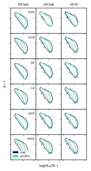
Figure 2: Superposition of the predicted (green) and the real (blue) Hi richness of our galaxies (x-axes) vs. $g-r$ colour (y-axes). The contours are enclosing $2\sigma$ of the distributions. Each row shows different mapping corresponding a particular method and each column a different setup (see Table 1).

For a given trained model (see §3), we can predict the Hi richness of a test set which contains the feature parameters, similar to those used during the training, and the real Hi richness. One can then see for a given example (composed by the features) how the model estimates the corresponding Hi richness and compare the predicted value of this latter with its real value. Figure 2 shows the galaxies’ M${}_{\textsc{Hi}}$/M_∗vs. a selected colour $g-r$, one of our input features. The simulated targets are shown with the blue contours and the predicted values with the green contours. Each column represents 3 selected setups (see Table 1) that only use SDSS magnitudes during the training whereas each row corresponds to one training model. The $z$-trained models shown here (two right columns: zSCmb, zSClr) are at $z=0$.

Overall, the ML-predicted values follow the true values from the simulation, and show that galaxy colour is anti-correlated with M${}_{\textsc{Hi}}$/M_∗ as expected. The mean trend is always well recovered using any of the predictors. However, the scatter in the data is not fully captured by any of the models: The green contours are always inside the blue contours. Different ML algorithms perform differently in this regard: We see that for DNN, RF & $k$NN, the two contours are quite close. Only looking at the $f$-trained models (left column) where we train on all the data from $z=0-2$ simultaneously, it is evident visually that RF maps $g-r$ best, $k$NN comes next followed by DNN. For the $z$-trained models where we train individually at various redshifts, DNN, RF & $k$NN do similarly well with zSCmb but the performance of RF is better with zSClr (where we add in the color indices). In contrast, SVM, LR and GRAD have difficulty to capture the scatter in the data, hence their predictions tend to be more tightly confined around the mean. While we have shown this specifically for $g-r$, the results for other colours are similar, and typically show that RF and DNN perform the best, with kNN not far behind.

Figure 3 shows a direct comparison between the real and the predicted Hi richness of the galaxies with the DNN models trained and tested with $z=0$ simulated data. The dashed line shows the 1:1 line; if the ML algorithm were perfect, all points would lie along this line. The correlation is apparent and generally follows the identity line, indicating that the training performs reasonably well in the mean. However, there is a significant scatter, which degrades the performance on a galaxy-by-galaxy basis. The best-fit slope is also not identically unity, so the correlation is not perfect even in the mean. We thus would like to quantify our regressors’ performance using the slope and tightness of the correlation.

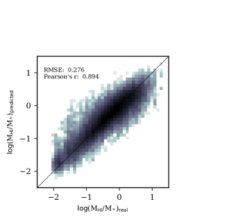
Figure 3: 2D distribution of the real (x-axis) vs. predicted (y-axis) Hi richness with the $z=0$-trained DNN model, using the zSCmb training set.

To quantify the performance of our ML framework, we choose three metrics:

• The slope of the linear mapping $f:y\rightarrow\hat{y}$, where an ideal mapping would have a unity slope.

• rmse (Root Mean Squared Error), given by

  $$\textsc{rmse}=\sqrt{{1\over{N}}\sum^{N}_{i=1}({y_{i}-\hat{y}_{i}})^{2}}$$

  where $y$ and $\hat{y}$ are the real value and the estimate respectively, gives the average difference between the predicted and the real values. The square of this metric is also used as a cost function to be minimized in some methods for regression ($e.g.$ deep neural network, linear regression). The lower the rmse the better the performance of the model is.

• Pearson product-moment correlation coefficient (Pearson’s r) which tells how scattered the predictions are compared to the true values. The closer to 1, the tighter (or better) the prediction is.

  $$\mathrm{Pearson^{\prime}s~{}r}={\sum_{i=1}^{N}(y_{i}-Y)(\hat{y}_{i}-\hat{Y})\over\sqrt{\sum_{i=1}^{N}(y_{i}-Y)^{2}}\sqrt{\sum_{i=1}^{N}(\hat{y}_{i}-\hat{Y})^{2}}}$$

  where $Y$ and $\hat{Y}$ are the mean values of $y_{i}$ and $\hat{y}_{i}$ respectively.

In figure 3, we get rmse$=0.276$ and Pearson’s r$=0.894$ for the particular choice of the DNN regressor and the zSCmb training set; this is one of our best cases, but RF is actually slightly better. Previous work by Zhang et al. (2009), estimating Hi-to-stellar mass ratio using analytic equation leads to $1\sigma$ scatter $>0.3$, which shows that our ML approach is more accurate.

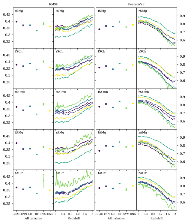
Figure 4: Root mean square errors RMSE and Pearson product-moment correlation coefficients r are shown on the 2 columns from the left and right, respectively. Models perform better if they show lower RMSE and higher r. The first on the left shows a mapping for all the galaxies, and the second for galaxies at different redshifts. The dots and lines are color coded by the training models we use. Each rows show different results for different setups. The rmse values are shown on the left y-axes and the r values on the right y-axes.

Figure 4 shows the performance of the various models considering each setup in Table 1 using rmse and Pearson’s r coefficient. The 2 columns from the left are the rmse and the 2 columns from the right are Pearson’s r. Each row corresponds to the results from different features used in the training. The name of the setup is shown on the top left of each panel. Different results from different learning techniques are presented with the color coded lines (with distinctive markers). In the following subsections we discuss how well our various regressors perform when varying the training set and the training method.

5.2 Dependence on redshift

Examining the leftmost column in Figure 4, these are the rmse’s for various ML algorithms when training on the entire data set from $z=0-2$ without any redshift information ($f$-training). The results bear out the trends noted in Figure 2: The RF method generally does the best (lowest rmse) for any of the input data sets, while DNN and kNN follow, and then the remaining methods. The RF values are still typically above 0.3, with the lowest values for the fSCmb (SDSS colours, magnitudes, and environment) and perhaps marginal improvement in fAMg which adds the near-IR photometry.

The third column shows the corresponding Pearson’s r values. The basic story is the same, that RF provides the best prediction, with values of r $\approx 0.85$ in the best cases, with others down to r $\approx 0.75$. The predictions from the aggregate dataset clearly contain significant information, but are perhaps not as optimal as one might get from including some redshift information.

The second and fourth columns show the result of training and testing at individual redshifts ($z$-training). It is clear that from $z\sim 0-0.5$, the $z$-training performs better than the aggregate ($f$) training, with lower rmse around 0.25 in the best-case RF models (zSCmb and zAMg). The other ML algorithms are clearly poorer than RF, although DNN does reasonably well in the zSCmb case. Similarly, the fourth column showing the Pearson’s r also is very good at $z=0-0.5$, and here DNN in many cases does nearly as well as RF.

Beyond $z>0.5$, all the regressors show degrading performance, with increasing rmse and decreasing r. This increase in rmse likely owes to the fact that at high-$z$, all galaxies are more Hi rich (M${}_{\textsc{Hi}}$/M_∗$>10^{-2}$) Rafieferantsoa et al. (2015), with fewer and fewer quenched galaxies with very low M${}_{\textsc{Hi}}$/M_∗. Because the intrinsic M${}_{\textsc{Hi}}$/M_∗ vs. mass (and other properties) thus becomes fairly flat, it becomes increasingly difficult for the ML to pick out the correct M${}_{\textsc{Hi}}$/M_∗ based on other galaxy properties as would be reflected in the photometry. This is likely an intrinsic limitation of this method, owing to the evolution of Hi in galaxies.

Redshift information can be obtained observationally, amongst other methods, from photometry or spectroscopy. The latter is still easier to retrieve than direct Hi data, while the former typically obtains redshift errors of a few percent, which is still good enough to ascribe a training redshift. It is clear from the above results that redshift information is useful to improve the predictions. Even out to $z\sim 1$, the limit of currently planned surveys, the predictions do not degrade greatly, it is only at $z>1$ that they become worse than the aggregate case. Hence from here on we will primarily discuss the $z$-training results.

5.3 Dependence on input features

The different rows in Fig. 4 show the impact of varying the input features into the ML framework. As we have seen, RF generally performs the best followed by DNN. GRAD, $k$NN, LR and SVM perform similarly poorly regardless of our setups (their rmse’s$\simeq 0.34$), with perhaps GRAD performing the worst. For this reason, unless otherwise stated, we are only going to discuss RF and DNN in what follows.

At $z=0$, using only SDSS magnitudes results in relatively poor performance, with rmse $\approx 0.3$ for RF and 0.35 for DNN and others. For RF, using either color indices instead of magnitudes (zSCls) or in addition to magnitudes (zSCmb) , or including additional magnitudes into the near-IR (zAMg) improves this significantly, with rmse as low as 0.25 and r$>0.9$. Thus it appears that providing colour information directly into the ML algorithm helps it determine a better mapping than only providing the magnitudes, even though in principle the magnitudes contain all the colour information. Also, providing additional near-IR bands seems to be advantageous.

For DNN, the story is slightly different. Again, only SDSS bands has the worst performance, but here, including the near-IR data does not improve things as much as providing color indices, and particularly providing both color indices and magnitudes together (zSCmb), which achieves a performance approaching that of RF.

The redshift dependence of rmse and r is similar among all these combinations of input datasets. The overall message is that providing more bands is better, which is unsurprising, but also that it is preferable to provide the colours directly rather than the magnitudes given the choice. In many cases, it is possible via SED fitting to obtain a galaxy colour that has uncertainties that are smaller than would be obtained by just subtracting magnitudes, so this may be a more valuable input for ML predictions.

5.4 The slope of the mean relation

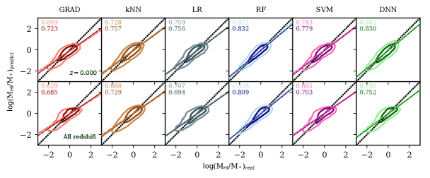
Figure 5: 2D representations of our real (x-axes) vs. predicted (y-axes) values of Hi richness. Upper panels show for different models at $z=0.0$, whereas the lower panels show for all redshift combined. We only show the results from our {f,z}SCmb features. The numbers with dark (light) colors on the left top corners show the slopes of the linear fit of the $1\sigma$ ($2\sigma$) subsample.

In Figure 5 we show linear fittings for the correlation between real (x-axis) and predicted (y-axis) values for M${}_{\textsc{Hi}}$/M_∗. The top pannels are for the $z$-trained models at $z=0$ and the lower panels for $f$-trained models. Each column corresponds to a given regressor as labeled on top. In each panel, the dark (light) lines represents the $1\sigma$ ($2\sigma$) contours between the targets and the predictions. The numbers on the top right are the slopes of the linear fits (color coded) for the two contours. The thick dashed line shows the 1-to-1 relation, which would be the perfect prediction. We only show the SDSS combined setup (zSCmb) here, i.e. the features are SDSS magnitudes+color indices +$v_{gal}$+$\Sigma_{3}$, but the results from other setups are similar.

We can see that $f$-trained (lower panels) models tend to have slopes further away from unity compared to those from the $z$-trained ones. This confirms what we found previously with rmse and Pearson’s r, that at low redshifts, training on the smaller but more homogeneous sample at a given $z$ provides a better prediction than training on a larger sample that conflates all the redshifts.

Among regressors, again we see that RF and DNN have slopes that are closest to unity, and thus perform better. All other methods have best-fit slopes below 0.8. However, all the slopes are $<1$, which indicates an under-prediction of the Hi richness for Hi rich galaxies and over-prediction for Hi-poor galaxies. This reflects the fact that, as seen in Figure 2, the true scatter in the M${}_{\textsc{Hi}}$/M_∗ around the mean is not fully reproduced in the predictions, such that all the regressors tend to fit galaxies closer to the mean. Hence at the lowest M${}_{\textsc{Hi}}$/M_∗, they tend to fit slightly higher values, while at the highest M${}_{\textsc{Hi}}$/M_∗, they tend to fit slightly lower values, resulting in a sub-unity slope: akin to an Eddington bias. The slope thus partly reflects a measure of how well the scatter around the mean is predicted. The fact that RF and DNN have the best slopes just quantifies the qualitative impression from Figure 2 that these regressors reproduce the extent of the scatter most closely.

Figure 6 shows the comparison of slope values for the $f$-trained sample (left panel) and the redshift evolution of the $z$-trained sample (right panel) among the various regressors. The left panel effectively just shows a plot depicting the numbers in the bottom row of Figure 5. Here, RF performs the best but not so far from DNN (considering the variance among 10 subsamples), and the other models perform somewhat worse.

The right panel extend the values shown in the upper panel of Figure 5 to higher redshift. Dark colors (or/and thick lines) show the $1\sigma$ slopes and the light colors (or/and thiner lines) show the $2\sigma$ slopes. Looking at the $z$-training results (right panel), it is very clear that the slopes of RF and DNN are closer to unity than the other models, and that is true across all redshifts. The $2\sigma$ slopes (light color lines) are generally better than the $1\sigma$’s, except at the lowest redshifts. Slopes $<0.5$ implies a weak correlation between the predicted and the real values of Hi richness, so Figure 6 indicates that all regressors become unreliable beyond $z\ga 1$.

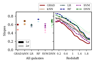
Figure 6: Slopes of the linear fit (y-axes) of the relationship between the predictions and the real Hi richness of our simulated galaxies. The dark color (or thick lines) show the fit for the $1\sigma$ sample around the maximum and the light color (or thin lines) for $2\sigma$. The left (x-axis showing the names of the models) is similar to what is shown in Figure 5 second row, the right (x-axis showing the redshift values) panel presents the evolution of slopes from our zSCmb features.

In summary, $k$-NN, RF and DNN methods show better performance as compared to SVM, GRAD and LR (Figure 2). DNN and RF tend to perform better when providing galaxy colours as opposed to photometry, and when providing more bands. Among our tests, the best mapping of Hi richness was achieved with RF at $z=0$ using optical and near-IR bands, which gave rmse’s $\approx 0.25$ and r $>0.9$. Using all data from $z=0-2$ together did not provide as a good fit as training at individual redshifts, despite the smaller samples for the latter. The evolution of rmse or Pearson’s r shows a stronger redshift dependence beyond $z\sim 0.5-1$ making the prediction uncertain at higher redshift ($z>1$, see Figure 4). Slopes of linear fits are generally less than unity owing to the fact that the true scatter is not fully spanned by the prediction; again, RF performs the best with DNN close behind, and the other regressors significantly poorer. All slopes move further from unity with increasing redshift, once again limiting applicability at $z\ga 1$.

6 Application to RESOLVE data

We now apply and test our ML methodology against real observations from the RESOLVE data. This survey provides both photometry and M${}_{\textsc{Hi}}$/M_∗, so provides an ideal sample to test the efficacy of our predictions. There are two ways we will test this: First, we will train on the RESOLVE data itself, and predict the RESOLVE data, to test how well it works in the ideal circumstance of having the training and testing set be from the same sample. Second, we will train on the simulation and predict the RESOLVE data, which is more like the application envisioned for this technique, to see how much degradation there is when the training and testing sets are different. If the simulation was a (statistically) perfect representation of the RESOLVE data, we would expect the resulting rmse and r to be similar, but given that we expect some differences, we aim to quantify the degredation in a real-world situation.

6.1 Simulated vs observed data

We first describe the RESOLVE data. We make use of the photometry data (Eckert et al., 2015) as well as their corresponding Hi-flux (Stark et al., 2016) from the Data Release ii@ of the RESOLVE survey. We use the following standard equation

$$M_{\mathrm{HI}}=2.36\times 10^{5}\times D^{2}\times F_{\mathrm{Total}}$$ (17)

to compute the Hi mass in $\;{\rm M}_{\odot}$, where $D$ is the distance to the galaxy (Mpc) calculated from the apparent and absolute magnitude in r band given in the photometry data. $F_{\mathrm{Total}}$, provided by the RESOLVE data, is the total Hi line flux ($Jy.\;{\rm km}\,{\rm s}^{-1}$) of the galaxy. The RESOLVE photometric data release contains SDSS (u,g,r,i,z), 2MASS (J,H,K), GALEX (NUV) and UKIDSS (Y,H,K) band magnitudes.

One immediate issue when comparing to simulations will be that stellar population models, initial mass function, etc. used to obtain $M_{*}$ from the data (from which we compute M${}_{\textsc{Hi}}$/M_∗) is different between what we assume in Loser versus what RESOLVE assumed to obtain their $M_{*}$ values. Hence it turns out there is a small offset in $M_{*}$ that we must first correct. We do so empirically, by using our ML framework to predict the $M_{*}$ from the photometry in our simulations and from RESOLVE, and then comparing the $M_{*}$ values.

Figure 7 (right panels), shows the difference between the original (top) and the corrected (bottom) M_∗ values from RESOLVE. The original RESOLVE data is offset by $\sim 0.1-0.2$ dex; this is within the uncertainties of typical $M_{*}$ determinations from photometry. The correction we apply is a linear scaling of the stellar masses to match with Mufasa galaxies, obtained by training the DNN model with the simulation to predict the stellar mass of the RESOLVE data, and comparing the result with the real value from RESOLVE. We repeat the process $10\times$ and take the average of the linear slopes and the intercepts, to obtain the following relation: $\log\mathrm{M}_{\mathrm{*,corrected}}=0.920\times\log\mathrm{M}_{\mathrm{*,original}}+0.924$. It can be seen that $M_{*}$ is predicted very tightly, with a scatter of rmse$=0.1$ once the correction is applied. Prior to the correction, the rmse$=0.22$ relative to the 1-to-1 line, which is dominated by the offset rather than the scatter itself. Note that scaling the simulated stellar masses would give the same results, but we don’t use this option because we know exactly the stellar mass of the simulated galaxies.

We can also compare the trend of M${}_{\textsc{Hi}}$/M_∗ vs. $M_{*}$ in the simulations and RESOLVE, which is done in the left panels of Figure 7, before (top) and after (bottom) the $M_{*}$ correction. The green-blue distributions on the left panels are from Mufasa-galaxies whereas the contours are from the observational data. In general, particularly after the correction is applied, the simulations and observations agree quite well for the bulk of the galaxies. A clear trend is seen that lower-$M_{*}$ galaxies have higher Hi fractions. The mean trend of the galaxies with Hi is in good agreement between RESOLVE and this simulation, which confirms the agreement versus other data sets shown in Rafieferantsoa et al. (2015). This indicates that Mufasa provides a generally viable model to predict observed Hi from photometry.

There is a notable difference that the observational data shows a bimodal distribution that is not seen in the simulated data. This is because we have explicitly ignored galaxies from Mufasa with M${}_{\textsc{Hi}}$/M_∗$<0.01$. In Mufasa, we have many galaxies with no Hi, while in the observations there is a distribution of low-M${}_{\textsc{Hi}}$/M_∗ values. We will leave more careful modeling of these low-M${}_{\textsc{Hi}}$/M_∗ objects for future work, but we note that the bimodality is going to degrade our results since the ML is unlikely to effectively predict galaxies with M${}_{\textsc{Hi}}$/M_∗ approaching $\sim 0.01$.

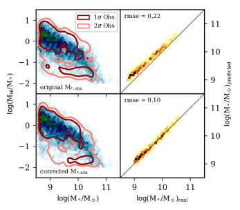
Figure 7: Left panels: The blue-green maps show the distribution of M_∗ (x-axes) vs. M${}_{\textsc{Hi}}$/M_∗ (y-axes) of the simulated galaxies, while the dark and light red contours show the 1 & 2 $\sigma$ distributions of the RESOLVE data. Right panels: distributions of the real (x-axes) and predicted (y-axes) galaxy stellar masses of the RESOLVE galaxies. Upper panels show the distributions prior to the correction to observed stellar masses as described in the text, and lower panels after correction. The lack of bimodality in the simulated data (right panels) as seen in the data is mainly due to our cut to only include galaxies with M${}_{\textsc{Hi}}$/M_∗$>10^{-2}$.

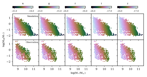
Figure 8: The x-axes and y-axes represent the stellar masses and Hi richness of the galaxies, respectively. Similar to bottom left panel of Figure 7, but showing the mean magnitudes in each pixel for the SDSS passbands (columns). The top and bottom panels are for simulated and observational data respectively. The agreement between the two data is noticeable and the range of the observational data are well included in that of the simulated ones.

We also check if the range of magnitudes between the RESOLVE and Mufasa are in broad accordance. Figure 8 shows the same distributions as in Figure 7 lower left panel, except that now the colours in each hexagonal bin represent the mean magnitudes of the galaxies in that bin. We show ugriz magnitudes for illustration but we get similar results for other bands. Each column represents one band. Upper and lower panels are for simulated and observational data respectively. We can clearly see that the trends are consistent. Note that apart from SDSS magnitudes, we also use NUV, J, H and $K_{s}$ magnitudes in the training. We however point that including all those bands decreases the size of the sample due to missing data in each band. The RESOLVE data contain $2159$ galaxies with SDSS magnitudes. When accounting for NUV, J, H and $K_{s}$ we end up with only $1017$ galaxies.

6.2 Training on and predicting RESOLVE data

We first consider the case where we train the regressors using one subset of the RESOLVE data and test them using the other subset (the one which was not used for the training). Due to the relatively small sample in hand, we only use 10% of the data for testing. This case can be considered optimal in the sense that the training and testing sets are drawn from (different parts of) the same sample, so there are no systematic differences.

The right panel on Figure 9 shows our prediction using the test sets. Judging by the contours, it is clear that all the presented models here perform reasonably well, i.e. the distribution of the real vs predicted values lie along the identity line, and the predicted values (y-axis) covers all the range of the real values for all regressors. Comparing regressors, GRAD with rmse$=0.28$ performs best followed closely by RF, $k$-NN and lastly DNN with rmse$=0.44$. Now the trend is reversed such that DNN, which was among the best in the previous scenario becomes the worst in this case. DNN’s typically require larger training samples to properly constrain the large number of layers, so it is likely its poor performance owes to the small sample of RESOLVE galaxies.

This result already has interesting real-world applications. For instance, it can be used to populate SDSS galaxies that lack Hi data or have poorly constrained Hi measurements with M${}_{\textsc{Hi}}$/M_∗ values. This would allow a reasonable characterisation of what their Hi content would be if RESOLVE had been able to observe them. Alternatively, one could use the larger ALFALFA sample cross-matched with SDSS data. By training the regressors on ALFALFA data along with their corresponding SDSS photometric data, we can predict the Hi content of galaxies that have SDSS photometric data but do not have ALFALFA counterparts. The key is that we need a single photometric sample, for which we have a training set of Hi data. In such a case, our method appears to be able to predict M${}_{\textsc{Hi}}$/M_∗ to $<0.3$ dex scatter, which is competitive with and typically better than previously proposed fitting formulae.

6.3 Training on Mufasa and predicting RESOLVE

A more general application would be where we have no or very limited Hi training data, and only photometric data. This might be the case at $z\sim 0.3-1$, where the Hi data is almost nonexistent now and even future surveys will provide only a sparse sampling of the most Hi-massive objects. In this case, we would like to be able to use the simulations to provide the training set. Naturally, this introduces more uncertainties and assumptions, because the simulations build in a specific physical model which likely is not exactly correct, and does not reproduce the real Hi population in all its details. To test how much more uncertain the predictions would be, we can attempt this using RESOLVE where we know what the correct answer is, and see how well the simulation recovers it relative to the case in the previous section where we used RESOLVE itself to train.

In order to mitigate the effects of those uncertainties, one must carefully mimic the input features of the simulated data to encompass those from the observational data as discussed in the previous section. Given that Mufasa reproduces several observables that are usually used as benchmark for simulation models, such as stellar mass function, Hi mass function, specific star formation rate function, etc. (Davé et al., 2016, 2017a, 2017b), we feel confident that it provides a state of the art approach to making predictions for upcoming surveys such as LADUMA or MIGHTEE, i.e. using simulated data for training the algorithms and applying it to available observational photometric data.

Figure 9, left panel, shows the Hi richness prediction of our four best models, training the regressors with the simulation data and predicted the Hi richness of the RESOLVE data. The contours show the distributions of the RESOLVE Hi richness (x-axis) vs the predicted Hi richness (y-axis) from the models. The numbers on the bottom right of each panel show the rmse of each model.

Overall, the predictions still lie along the one-to-one relation, indicating that using the simulations to train still provides an adequate prediction in the mean. However, the rmse values are much higher here than in the right panel. This clearly shows that the simulated sample does not fully mimic the details of the observed sample. Given the discrepancies between simulation and observation, implying differences of the underlying distributions of the two samples, this is not surprising.

$k$-NN, GRAD and RF now all have rmse values above 0.5, which is fairly poor. They estimate with larger scatter and a noticeable offset towards lower Hi richness values, where the contours get as far as 1 dex below the 1:1 line at log₁₀(M${}_{\textsc{Hi}}$/M_∗) $\sim 0$.

Rather remarkably, DNN (green contour) now performs the best in this case, with rmse = 0.45 and predictions extending to the lowest values ($-2\leq$) following the 1:1 line. Although DNN was outperformed in Figure 4 using only simulated data for training and testing, we can clearly see here that its performance shines in a more difficult scenario, where now the training sample is much larger but the data is more complex. Indeed, the rmse for DNN hardly changed at all when using the RESOLVE or Mufasa data to train, though this probably arises from the larger training sample offsetting the less homogeneous testing sample. Our results suggest that in this real-world application, DNN can learn better from the simulated data than simpler regressors.

From those two approaches, left and right panels of Figure 9, we can see that DNN presents robust predictions regardless of the training setups. It is able to learn important features from the simulation and translate those into the observed data. kNN, GRAD and surprisingly RF are less efficient in doing so. The latter only performs best when the training and testing samples are drawn from the same main sample.

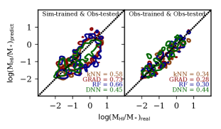
Figure 9: Predictions of the observed Hi richness (y-axes) using different mapping algorithms (colour coded lines). Left panel shows the results when the algorithms are trained with simulated data. Right panel shows the results when training the algorithms with observational data. The contours correspond to 1$\sigma$ distribution.

To summarize, we have shown that training on a subset of observational data can yield a reasonably tight prediction for a testing set taken from the same data. This provides a way to populate photometric surveys in scenarios where a sizeable Hi training set is available, such as RESOLVE or ALFALFA. Training the models with simulated data and predicting the observational targets has higher uncertainties, but is still feasible. One has to carefully model the input features from the simulation to mimic those in the data, which requires further work. While RF has generally been the best choice for regressor in more homogeneous training-test set situations (simulation-simulation and observation-observation), when applying the simulation training to observational data, the performance of DNN clearly outshined the others.

7 Discussion

Extraction of information in a given set of data is a challenge in all models. Although RF and DNN are our best models, they still have difficulty in extracting all the necessary information, particularly DNN. That being said, attaining an accuracy of r $>85\%$ is a non trivial success for both of regressors. In our training for the DNN, we make sure that the loss function stays unchanged for several training steps to make sure the network learns as much information as it needs but not as much as it might overfit the training data and loose the important information necessary for the prediction. It may be possible to tune this better.

It is possible that photometric surveys can yield other information such as the age, star formation rate, and (from a group catalog) halo masses, albeit with some uncertainties. It is interesting to ask whether providing such information would improve predictions. However, we find that this is unlikely to be the case. We illustrate this for the mean stellar age in Figure 10. Here we show the distribution of the galaxies based on their real Hi richness and the predicted values from the DNN model, with the colour of each hexagonal bin showing the mean age of galaxies falling in that bin (in unit of the Hubble time at the given redshift). Different panel show different redshifts: left, center, right for $z=\{0,1,2\}$ respectively. We can see that for a given Hi richness value we cannot see any age gradient in the predicted values, and it remains the case up to $z=2$. We interpret this to mean the ML model has learned about the age of the galaxies even though that information was not explicitly given in the training set. The same situation happens with the specific star formation rates and the halo mass of the galaxies. This is the case for all of our ML models. Hence providing such information, which introduces further uncertainties from their estimation, is unlikely to be helpful.

Then we might ask why do some models perform better than others? We believe that the design of the models themselves may lead to different mapping of the input-output, thus, to improved results depending on the data. Changing the layer structures in DNN or optimising the tree size (or the number of base estimators) in RF might alleviate certain issues we encountered in our training. We are currently analyzing such possibility and might improve our model in that direction in upcoming work. Also DNN may particularly benefit from a larger simulation training sample with more dynamic range than available in Mufasa.

One useful feature of RF is that it provides an estimate of the importance level of the input parameters, based on the rate of incidence that a given parameter is utilised in the decision trees. We show in Figure 11 the importance of parameters from RF training. The upper subfigure shows the result when using all the available magnitudes in from our simulation whereas the lower subfigure represents the result when only using the SDSS magnitudes. The 1^st (2^nd) row in each subfigure show the importance of the line of sight velocity $v_{gal}$ (3^rd nearest neighbour $\Sigma_{3}$) from $z=0$ (left) to $z=2$ (right). The remaining rows show for bandpass filters (names on the left) with a wide range of peak wavelenghts from 2309Å (bottom row) increasing to 44630Å. It is interesting to see that $\Sigma_{3}$ becomes increasingly important only at later epochs. The line of sight peculiar velocities $v_{gal}$ do not add value to the training, which is unsurprising since it is not obvious why the Hi content should care about peculiar velocity (except perhaps through correlations of peculiar velocities and the large-scale potential well); this in a sense serves as a sanity check that our method is not finding physically implausible relationships. In the upper subfigure, the IRAC channels have some importance at higher redshift, particular IRAC $4.5\mu m$ while $3.6\mu m$ is less important. The H-band magnitude is very important at high redshift but contributes much less at low redshift. The importance of magnitudes between i ($6250\AA$) and J ($12500\AA$) bands move from low to higher peak wavelengths towards higher redshift. NUV magnitudes seem to exhibit relatively high importance at all redshift bins, highlighting the connection between Hi and the gas that fuels star formation and hence UV light.

In the lower subfigure with a more restricted input set, $z$ magnitude is very important at higher redshift but becomes less although still important at $z=0$, whereas the importance of $i$ magnitude increases towards the present day. The value that $u$ magnitude adds to the accuracy of the prediction seems to be relatively constant at all redshifts, following NUV in the upper subfigure.

On the whole what the two panels in Figure 11 tell us is that given the features available in the data, the feature importance in principle allows one to select only a set of the most important ones in order to achieve a given accuracy. This, amongst other methods like Principal Component Analysis (PCA), is of a great value especially when reducing the dimensionality that might not be avoidable due to a limited computing power or when the dimension is as big as the size of the data (i.e. number of features is as large as the number of examples for the training). Also, the importance levels could be helpful in survey design, if a particular photometric band is more useful it might be regarded as higher priority to obtain. However, one must be aware that in many cases, RF importance levels do not truly reflect the necessity of a given data, in the sense that sometimes RF says a particular input is important, but the information from that input is actually encoded in the other inputs, so that removing it does not have as detrimental effect as one might think. Properly assessing the importance level would involve re-training the entire data set removing each input in turn, to assess the increase in rmse. Nonetheless, RF importance level can at least provide a guide in this process.

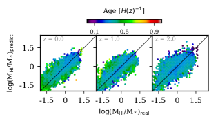
Figure 10: Mean galaxy age for each pixel in the distribution of the real (x-axes) and predicted (y-axes) Hi richness of the simulated galaxies. This result is from the DNN-trained model. Different panels show for different redshift. We use the age of the galaxies at the given redshifts (shown on the top left corner in each panel).

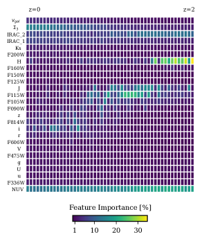
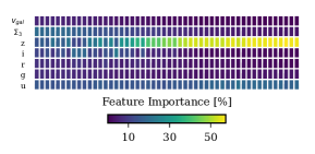
Figure 11: Evolution of the importance of the input features from the RF training. Each row represents one band with the filter name on the left, except for the 1^st (2^nd) row which show for the line of sight velocity (3^rd nearest neighbour) feature. The bands from the bottom to the top are with increasing peak wavelengths. Left to the right shows the feature importance from $z=0$ to $z=2$.

8 Conclusion

We have investigated estimating the Hi richness of galaxies based on their optical and near-IR survey properties, in particular SDSS $\{u,g,r,i,z\}$, Johnson $\{U,V\}$ and 2MASS $\{J,H,K_{s}\}$, line of sight velocities, and environmental measures, using machine learning (ML). For our analysis, the training data have been generated from the Mufasa simulation. We have tested various machine learning regressors including random forests and deep neural networks. We considered various input feature combinations, including only SDSS magnitudes and environmental properties, using galaxy colours instead of and in addition to magnitudes, and including 2MASS and Johnson magnitudes. We trained each model to predict M${}_{\textsc{Hi}}$/M_∗ based on an aggregate of all simulated galaxies at $z=0-2$ ($f$-training), and in 50 individual redshift bins ($z$-training). As an example application, we applied this framework to the RESOLVE galaxy survey catalog with Hi and photometric data. To measure and compare the performance of each method, we used rmse, Pearson correlation coefficient r , and the correlation slope.

We summarize our main findings as follows:

• By using 75% of the Mufasa data for training and testing on the remaining quarter, we find that all ML methods are able to approximately recover M${}_{\textsc{Hi}}$/M_∗ from galaxy photometry. The accuracy depends both on the input data set and the ML algorithm. Generally, random forests (RF) provides the best performance at $z=0$, i.e. lowest rmse $\approx 0.25$, highest r $\approx 0.9$, and slope closest to unity, with deep neural network (DNN) close behind.

• At $z\la 1$, it is advantageous to do the ML training at a given redshift rather than aggregating all redshifts. The smaller number of galaxies available for training in the former is outweighed by the conflating of evolutionary trends when aggregating. The rmse of all ML algorithms increases with redshift, with commensurately lowered r and a best-fit slope diverging from unity, though the effect is mild out to $z\sim 0.5$. Predictions at higher redshifts are more challenging owing to reduced trend in M${}_{\textsc{Hi}}$/M_∗ among high-$z$ galaxies, since most galaxies at $z\ga 1$ have similar M${}_{\textsc{Hi}}$/M_∗ prior to significant populations of quenched galaxies arising.

• Providing more input training data results in better predictive power, unsurprisingly. Using only SDSS data results in rmse$\approx 0.3$ for RF at $z=0$, while either including 2MASS data or training on both colours and magnitudes yields a more optimal rmse. DNN has in the best case similar performance, but it is more strongly dependent on the selected input features.

• All the regressors tend to under-predict the high Hi richness and over-predict the low Hi richness, as shown by the slope ($<1$) of the linear fits between the targets and the predictions. This owes to the regressors being unable to fully capture the scatter in the M${}_{\textsc{Hi}}$/M_∗ values at e.g. a given colour, instead tending to push the M${}_{\textsc{Hi}}$/M_∗ towards the mean. This raises the value of low M${}_{\textsc{Hi}}$/M_∗ objects and lowers it for high M${}_{\textsc{Hi}}$/M_∗ objects, resulting in a sub-unity slope. The under-prediction of the high Hi richness is more severe at high redshift (Figure 6).

• By training our ML framework on a subset of the RESOLVE data and testing it on the remainder, we showed that it is possible to predict M${}_{\textsc{Hi}}$/M_∗ with rmse $\approx 0.3$, which is comparable or better than what is obtained with scaling laws; RF again performs among the best, though GRAD is slightly better. When training on Mufasa and testing on RESOLVE, we find the best regressor is DNN, but the predictions are significantly degraded with rmse$\approx 0.45$, likely owing to subtle mismatches between simulation predictions and analysis procedures and those from RESOLVE. While the scatter is substantial, the mean trend remains well-matched, showing that the ML algorithm introduces only mild systematic biases, and thus is still valuable for statistical survey applications.

We have shown through this study that it is clearly possible to estimate the Hi  richness of a galaxy by relying only on the information from photometric magnitudes. We considered various magnitudes from different surveys like SDSS, Johnson and 2MASS in this work, but including other bands is doable. The broadly successful test on RESOLVE data suggests that the estimation of Hi gas at higher redshift (being $z\leq 1$) using the methods presented here, even with the lack of testing data, is sensible. With the advent of future surveys such as LADUMA and MIGHTEE, our ML framework constitutes an important new tool to aid studies of neutral hydrogen and galaxy evolution.

For our analysis, we have only selected galaxies that are observable in Hi, with a threshold of M${}_{\textsc{Hi}}$/M_∗$>10^{-2}$. This raises a key question:"Would a model still generalize well if one also included the Hi-depleted galaxies in the dataset for the training?". There are two ways to address this question:

• We can simply add the Hi-deficient galaxies in the dataset and redo the fitting procedure prescribed in this work, although from the standpoint of observations, predicting the Hi richness of a Hi-depleted or gas-starved galaxy is not really meaningful.

• The more elegant approach would be to first use ML to classify galaxies based on their observable features whether they are Hi deficient or not, then only estimate its Hi richness (based on the same features) in the case it would potentially contain observable Hi. Of course, the minimal value of observed Hi  can be a free parameters in our model but in reality that should depend on the telescope capabilities.

Future work will discuss these solutions, provide more tailored predictions for upcoming surveys, utilise larger training samples that could particularly help improve DNN results, and make this tool available to the community.

References

- Altman (1992) Altman N. S., 1992, j-AMER-STAT, 46, 175
- Breiman (2001) Breiman L., 2001, Mach. Learn., 45, 5
- Catinella et al. (2010) Catinella B., et al., 2010, MNRAS, 403, 683
- Catinella et al. (2013) Catinella B., et al., 2013, MNRAS, 436, 34
- Conroy & Gunn (2010) Conroy C., Gunn J. E., 2010, FSPS: Flexible Stellar Population Synthesis, Astrophysics Source Code Library (ascl:1010.043)
- Cortes & Vapnik (1995) Cortes C., Vapnik V., 1995, Machine Learning, 20, 273
- Crain et al. (2009) Crain R. A., et al., 2009, MNRAS, 399, 1773
- Croton et al. (2006) Croton D. J., et al., 2006, MNRAS, 367, 864
- Cunnama et al. (2014) Cunnama D., Andrianomena S., Cress C. M., Faltenbacher A., Gibson B. K., Theuns T., 2014, MNRAS, 438, 2530
- Cybenko (1989) Cybenko G., 1989, Mathematics of Control, Signals and Systems, 2, 303
- Davé et al. (2013) Davé R., Katz N., Oppenheimer B. D., Kollmeier J. A., Weinberg D. H., 2013, MNRAS, 434, 2645
- Davé et al. (2016) Davé R., Thompson R., Hopkins P. F., 2016, MNRAS, 462, 3265
- Davé et al. (2017a) Davé R., Rafieferantsoa M. H., Thompson R. J., Hopkins P. F., 2017a, MNRAS, 467, 115
- Davé et al. (2017b) Davé R., Rafieferantsoa M. H., Thompson R. J., 2017b, MNRAS, 471, 1671
- Duffy et al. (2012) Duffy A. R., Kay S. T., Battye R. A., Booth C. M., Dalla Vecchia C., Schaye J., 2012, MNRAS, 420, 2799
- Eckert et al. (2015) Eckert K. D., Kannappan S. J., Stark D. V., Moffett A. J., Norris M. A., Snyder E. M., Hoversten E. A., 2015, ApJ, 810, 166
- Friedman (2000) Friedman J. H., 2000, Annals of Statistics, 29, 1189
- Gabor & Davé (2015) Gabor J. M., Davé R., 2015, MNRAS, 447, 374
- Giovanelli et al. (2005) Giovanelli R., et al., 2005, AJ, 130, 2598
- Hahn & Abel (2011) Hahn O., Abel T., 2011, MNRAS, 415, 2101
- Hastie et al. (2009) Hastie T., Tibshirani R., Friedman J., 2009, The elements of statistical learning: data mining, inference and prediction, 2 edn. Springer, http://www-stat.stanford.edu/~tibs/ElemStatLearn/
- Hinton et al. (2006) Hinton G. E., Osindero S., Teh Y.-W., 2006, Neural Computation, 18, 1527
- Holwerda et al. (2012) Holwerda B. W., Blyth S.-L., Baker A. J., 2012, in Tuffs R. J., Popescu C. C., eds, IAU Symposium Vol. 284, The Spectral Energy Distribution of Galaxies - SED 2011. pp 496–499 (arXiv:1109.5605), doi:10.1017/S1743921312009702
- Hopkins (2015) Hopkins P. F., 2015, MNRAS, 450, 53
- Hornik (1991) Hornik K., 1991, Neural Networks, 4, 251
- Jones et al. (2016) Jones M. G., Papastergis E., Haynes M. P., Giovanelli R., 2016, MNRAS, 457, 4393
- Kannappan (2004) Kannappan S. J., 2004, ApJ, 611, L89
- Kannappan et al. (2011) Kannappan S., et al., 2011, in American Astronomical Society Meeting Abstracts #217. p. 334.14
- Kereš et al. (2005) Kereš D., Katz N., Weinberg D. H., Davé R., 2005, MNRAS, 363, 2
- Kingma & Ba (2014) Kingma D. P., Ba J., 2014, CoRR, abs/1412.6980
- Krumholz & Gnedin (2011) Krumholz M. R., Gnedin N. Y., 2011, ApJ, 729, 36
- Mitra et al. (2015) Mitra S., Davé R., Finlator K., 2015, MNRAS, 452, 1184
- Muratov et al. (2015) Muratov A. L., Keres D., Faucher-Giguere C.-A., Hopkins P. F., Quataert E., Murray N., 2015, ArXiv e-prints:1501.03155,
- Pedregosa et al. (2011) Pedregosa F., et al., 2011, Journal of Machine Learning Research, 12, 2825
- Planck et al. (2016) Planck et al., 2016, A&A, 594, A13
- Quilis et al. (2017) Quilis V., Planelles S., Ricciardelli E., 2017, MNRAS, 469, 80
- Rafieferantsoa & Davé (2018) Rafieferantsoa M., Davé R., 2018, MNRAS, 475, 955
- Rafieferantsoa et al. (2015) Rafieferantsoa M., Davé R., Anglés-Alcázar D., Katz N., Kollmeier J. A., Oppenheimer B. D., 2015, MNRAS, 453, 3980
- Rahmati et al. (2013) Rahmati A., Pawlik A. H., Raičevic̀ M., Schaye J., 2013, MNRAS, 430, 2427
- Schmidt (1959) Schmidt M., 1959, ApJ, 129, 243
- Somerville & Davé (2015) Somerville R. S., Davé R., 2015, ARA&A, 53, 51
- Springel (2005) Springel V., 2005, MNRAS, 364, 1105
- Stark et al. (2016) Stark D. V., et al., 2016, ApJ, 832, 126
- Vapnik (1995) Vapnik V. N., 1995, The nature of statistical learning theory. Springer-Verlag New York, Inc., New York, NY, USA
- Wang et al. (2011) Wang J., et al., 2011, MNRAS, 412, 1081
- Wang et al. (2013) Wang J., et al., 2013, MNRAS, 433, 270
- Wang et al. (2015) Wang E., Wang J., Kauffmann G., Józsa G. I. G., Li C., 2015, MNRAS, 449, 2010
- York et al. (2000) York D. G., et al., 2000, AJ, 120, 1579
- Zhang et al. (2009) Zhang W., Li C., Kauffmann G., Zou H., Catinella B., Shen S., Guo Q., Chang R., 2009, MNRAS, 397, 1243