Learning through deterministic assignment of hidden parameters

Abstract

Supervised learning frequently boils down to determining hidden and bright parameters in a parameterized hypothesis space based on finite input-output samples. The hidden parameters determine the nonlinear mechanism of an estimator, while the bright parameters characterize the linear mechanism. In traditional learning paradigm, hidden and bright parameters are not distinguished and trained simultaneously in one learning process. Such an one-stage learning (OSL) brings a benefit of theoretical analysis but suffers from the high computational burden. In this paper, we propose a two-stage learning (TSL) scheme, learning through deterministic assignment of hidden parameters (LtDaHP), where we suggest to deterministically generate the hidden parameters by using minimal Riesz energy points on a sphere and equally spaced points in an interval. We theoretically show that with such deterministic assignment of hidden parameters, LtDaHP with a neural network realization almost shares the same generalization performance with that of OSL. Then, LtDaHP provides an effective way to overcome the high computational burden of OSL. We present a series of simulations and application examples to support the outperformance of LtDaHP.

I Introduction

In physical or biological systems, engineering applications, financial studies, and many other fields, only can finite number of samples be obtained. Supervised learning aims at synthesizing a function (or mapping) to represent or approximate an unknown but definite relation between the input and output, based on the input-output samples. The learning process is accomplished with the selection of a hypothesis space and a learning algorithm. The hypothesis space is a family of functions endowed with certain structures, very often, a space spanned by a set of parameterized functions like

$$\mathcal{H}=span\left\{\psi(\xi_{j},x):\xi_{j}\in\Omega,j=1,2,\dots,N\right\}$$ (1)

where $\xi_{j}$ is a parameter for specifying the $j$-th function $\psi_{j}(\cdot):=\psi(\xi_{j},\cdot)$ and $\Omega$ is a class of parameters. A typical example is the three-layer feed-forward neural networks (FNNs) in which $\psi(\xi_{j},x)$ is the response of the $j$-th neuron in the hidden layer with $\xi_{j}$ being all the connection weights connected to the neurons [13]. A learning algorithm is then defined by some optimization scheme to derive an estimator in $\mathcal{H}$ based on the given samples. To distinguish the type of parameters, we call each $\psi_{j}(\cdot):=\psi(\xi_{j},\cdot)$ a hidden predictor, $\xi_{j}$ a hidden parameter, and $a_{j}$ a bright parameter. Then, for a nonlinear function $\psi$, it follows from (1) that hidden parameters determine the attributions of hidden predictors of the estimator ( nonlinear mechanism), while bright parameters characterize how hidden predictors are linearly combined (linear mechanism). In this sense, supervised learning boils down to determining hidden and bright parameters in a parameterized hypothesis space.

In traditional learning paradigm, hidden and bright parameters are not distinguished and trained simultaneously. Such a scheme is featured as the one-stage learning (OSL). The well known support vector machine (SVM) [45], kernel ridge regression [9] and FNNs [13] are typical examples of the OSL scheme. OSL has a benefit of theoretical attractiveness in the sense that this scheme enables to realize the optimal generalization error bounds [32, 44, 26]. However, it inevitably requires to solve some nonlinear optimization problem, which usually suffers from the time-consuming difficulty, especially for problems with large-sized samples.

To circumvent this difficulty, a two-stage learning (TSL) scheme, featured as learning through random assignment of hidden parameters (LtRaHP), was developed and widely used [4, 17, 18, 29, 35] in the last two decades. LtRaHP assigns randomly the hidden parameters in the first stage and determines the bright parameters by solving a linear least-square problem in the second stage. Typical examples of LtRaHP include, the random vector functional-link networks (RVFLs) [35], the echo-state neural networks (ESNs) [18], the random weight neural networks (RWNNs) [4] and the extreme learning machine (ELM) [17]. LtRaHP significantly reduces the computational burden of OSL without sacrificing the prediction accuracy very much, as partially justified in our recent theoretical studies [24, 28]. However, due to the randomness of the hidden parameters, a satisfactory generalization capability of LtRaHP is achieved only in the sense of expectation. This then leads to an uncertainty problem: it is uncertain whether a single trail of the scheme succeeds or not. Consequently, to yield a convincing result, multiple times of trails are required in the training process of LtRaHP.

From these studies, we draw a simple conclusion on the pros and cons of existing learning schemes. OSL possesses promising generalization capabilities but it is built on the high computational burden, while LtRaHP has charming computational advantages but it suffers from an uncertainty problem. Thus, it is still open to find an efficient and feasible learning scheme, especially when the size of data is huge. Our aim in the present paper is to develop a new TSL scheme. Our core idea is to apply a deterministic mechanism for the assignment of hidden parameters in place of the random assignment in LtRaHP. Accordingly, the new TSL scheme will be featured as learning through deterministic assignment of hidden parameters (LtDaHP). We will show that LtDaHP outperforms LtRaHP in the sense that LtDaHP avoids the uncertainty problem of LtRaHP without increasing the computational complexity.

As the popularity of neural networks in recent years [10, 36, 7, 48], we equip the LtDaHP scheme with an FNN-instance to show its outperformance. Taking inner weights as minimal Riesz energy points on a sphere and thresholds as equally spaced points (ESPs) in an interval, we can define an FNN-realization of LtDaHP. We theoretically justify that so defined LtDaHP outperforms both LtRaHP and OSL in many ways. Firstly, LtDaHP can achieve the almost optimal generalization error bounds of the OSL schemes; Secondly, LtDaHP significantly reduces the computational burden of OSL; Finally, unlike LtRaHP, LtDaHP can find a satisfactory estimator in a single time of trial. Thus, LtDaHP provides an effective way of overcoming both the high computational burden difficulty of OSL and the uncertainty problem of LtRaHP. We also provide a series of simulations and application examples to support the outperformance of LtDaHP.

The rest of paper is organized as follows. Section II aims at introducing the new FNN-realization of LtDaHP as well as a brief introduction of the minimal Riesz energy configuration problem on the sphere. In Section III, we verify the almost optimality of LtDaHP in the framework of statistical learning theory. In Section IV, we provide the simulations and application examples to support the outperformance of LtDaHP and the correctness of the theoretical assertions we have made. We conclude the paper in Section V with some remarks.

II FNN-Realization of LtDaHP

In this section, after providing the motivation of the LtDaHP scheme and briefly introducing minimal Riesz energy points on the sphere, we formalize an FNN-realization of LtDaHP.

II-A Motivations

FNNs, taking three-layer FNNs with one output neuron for example, look for the estimators of the form $f_{FNN}(x)=\sum_{j=1}^{N}a_{j}\phi(\alpha_{j}\cdot x-b_{j})$ where $\alpha_{j}$ is the inner weight which connects the input layer to the $j$-th hidden neuron, $b_{j}$ is the threshold of the $j$-th hidden neuron, $\phi$ is the nonlinear activation function, and $a_{j}$ is the outer weights that connects the $j$-th hidden layer to the output layer. In FNNs, the hidden parameters are $\{\alpha_{j},b_{j}\}_{j=1}^{N}$ and the bright parameters are $\{a_{j}\}_{j=1}^{N}.$ FNNs generate their estimators conventionally through solving the optimization problem

$$\min_{(a_{j},\alpha_{j},b_{j})\in\mathbb{R}^{1}\times\mathbb{R}^{d}\times\mathbb{R}^{1}}\sum_{i=1}^{m}\left|\sum_{j=1}^{N}a_{j}\phi(\alpha_{j}\cdot x_{i}-b_{j})-y_{i}\right|^{2}.$$ (2)

It is obvious that (2) does not distinguish hidden parameters and bright parameters and is actually an OSL.

Our idea to design a TSL learning system based on FNNs mainly stems from two interesting observations. On the one hand, we observe in theoretical literature [37, 30] that to realize the optimal approximation capability, the inner weights of an FNN can be restricted on the unit sphere embedded into the input space. This theoretical finding provides an intuition to design efficient learning schemes based on FNNs with shrinking the class of parameters. On the other hand, the existing LtRaHP schemes [17, 18, 28, 35] shows that the uniform distribution for hidden parameters is usually effective. This prompts us to assign the hidden parameters as uniform as possible. An extreme assignment is to deterministically select the hidden parameters as the equally spaced points (ESPs), rather than the random sketching. Combining these two observations, it is reasonable to generate inner weights as ESPs on the unit sphere and thresholds as ESPs on some interval.

The problem is, of course, can ESPs on the sphere be practically constructed? This problem, known as the Tamme’s problem or the hard sphere problem [40], is a well known and long-standing open question. This perhaps explains why only LtRaHP has been widely utilized in TSL up to now, even though several authors have already conjectured that LtDaHP may outperform its random counterpart [15]. However, due to the non-boundary property of the sphere, the Tamme’s problem is the limiting case of another famous problem: The minimal Riesz energy configuration problem [41]. The latter problem, listed as the $7$-th problem of Smale’s “problems for this century” [42], can be approximately solved by using several methods, such as the equal-area partition [41] and recursive zonal sphere partitioning [22]. Thus, the hidden parameters of FNNs can be selected by appropriately combining the minimal Riesz energy points on the sphere with the equally spaced points in an interval.

II-B Minimal Riesz energy points on the sphere

Let $\mathbb{S}^{d-1}$ denote the unit sphere in the $d$-dimensional Euclidean space $\mathbb{R}^{d}$, and $\Xi_{n}:=\{\xi_{1},\dots,\xi_{n}\}$ be a collection of $n$ distinct points (a configuration) on $\mathbb{S}^{d-1}$. The Riesz $\tau$-energy $(\tau\geq 0)$ associated with $\Xi_{n}$, denoted by $A_{\tau}(\Xi_{n})$, is defined by [16]

$$A_{\tau}(\Xi_{n}):=\left\{\begin{array}[]{cc}\sum_{i\neq j}|x_{i}-x_{j}|^{-\tau},&if\ \tau>0,\\ \sum_{i\neq j}-\log|x_{i}-x_{j}|,&if\ \tau=0.\end{array}\right.$$

Here $|\cdot|$ is the Euclidean norm. We use $\mathcal{E}_{\tau}(\mathbb{S}^{d-1},n)$ to denote the $n$-point minimal $\tau$-energy over $\mathbb{S}^{d-1}$, that is,

$$\mathcal{E}_{\tau}(\mathbb{S}^{d-1},n):=\min_{\Xi_{n}\in\mathbb{S}^{d-1}}A_{\tau}(\Xi_{n}),$$ (3)

where the minimization is taken over all $n$-point configurations of $\mathbb{S}^{d-1}$. If $\Xi_{n}^{\ast}\subset\mathbb{S}^{d-1}$ is a minimzer of (3), i.e.,

$$A_{\tau}(\Xi_{n}^{\ast})=\mathcal{E}_{\tau}(\mathbb{S}^{d-1},n),$$

then $\Xi_{n}^{\ast}$ is called a minimal $\tau$-energy configuration of $\mathbb{S}^{d-1}$, and the points in $\Xi_{n}^{\ast}$ are called the minimal $\tau$-energy points.

The elegant work in [21] showed that the minimal $\tau$-energy points of $\mathbb{S}^{d-1}$ are an effective approximation of the equally spaced points (ESPs) on the sphere whenever $\tau\geq d-1$. Thus, one can use the minimal $\tau$-energy points to substitute ESPs in applications. As formulated as the Smale’s $7th$ problem [42], generating minimal $\tau$-energy configurations and minimal $\tau$-energy points on $\mathbb{S}^{d-1}$ has triggered enormous research activities [16, 22, 41] in the past thirty years.

Up till now, there have been several well established approaches to approximately solve the minimal $\tau$-energy configuration problems [19, 22, 41], among which two widely used procedures are Saff et al.’s equal-area partitioning [41] and Leopardi’s recursive zonal sphere partitioning procedure [22]. Both of them have been justified to be able to approximately generate the minimal $\tau$-energy points of $\mathbb{S}^{d-1}$ for a certain $\tau$ with a “cheap” computational cost, more precisely, with an $\mathcal{O}(n\log n)$ asymptotic time complexity [22].

II-C The LtDaHP Scheme

Let ${\bf z}=\{(x_{i},y_{i})\}_{i=1}^{m}$ be the set of samples with $x_{i}\in X$ and $y_{i}\in Y$. Without loss of generality, we assume the input space $X=\mathbb{B}^{d}$ and the output space $Y\subseteq[-M,M]$, where $\mathbb{B}^{d}$ is the unit ball in $\mathbb{R}^{d}$ and $M>0$. Our idea is to solve an FNN-learning problem by the TSL approach which deterministically assigns the hidden parameters at the first stage, and solves a linear least-square problem at the second stage. In particular, we propose to deterministically assign inner weights to be minimal Riesz $\tau$-energy points of $\mathbb{S}^{d-1},$ and thresholds to be ESPs in the interval $[-1/2,1/2].$ Consequently, our suggested FNN-realization of LtDaHP can be formalized as follows:

LtDaHP Scheme: Given the training samples ${\bf z}=(x_{i},y_{i})_{i=1}^{m}$, the nonlinear function $\phi$ and a splitting $N=n\ell,$ we generate the LtDaHP estimator via the following two stages:

Stage 1: Take the inner weights $\{\alpha_{j}\}_{j=1}^{n}$ to be minimal Riesz $\tau$-energy points of $\mathbb{S}^{d-1}$ with $\tau\geq d-1$,  and $\{b_{k}\}_{k=1}^{\ell}$ to be ESPs in the interval $[-1/2,1/2],$ that is,

$$b_{k}=-\frac{1}{2}+\frac{k}{\ell},\ k=1,2,\dots,\ell.$$

We then obtain a parameterized hypothesis space

$$\mathcal{H}_{\ell,n,\phi}:=\left\{\sum_{j=1}^{n}\sum_{k=1}^{\ell}a_{jk}\phi(\alpha_{j}x-b_{k}):a_{jk}\in\mathbb{R}^{1}\right\}.$$ (4)

Stage 2: The LtDaHP estimator is defined by

$$f_{\mathbf{z},\ell,n,\phi}:=\arg\min_{f\in\mathcal{H}_{\ell,n,\phi}}\frac{1}{m}\sum_{i=1}^{m}|f(x_{i})-y_{i}|^{2}.$$ (5)

Classical neural network approximation literature [6, 14, 3] shows that neural networks with fixed inner weights are sufficient to approximate univariate functions. We adopt this approach in our construction (4) by using $\sum_{k=1}^{\ell}a_{k}\phi(t-b_{k})$ to approximate univariate functions. Then, we use an approach from [37] to extend univariate approximation to multivariate approximation (see Section C in Appendix for detailed construction), which requires $n\sim\ell^{d}$ different inner weights on the sphere and obtained an FNN with good approximation property formed as (4). It should be mentioned that $\ell$ in the splitting is the main parameter to control the approximation accuracy and $n$ depends on $\ell$ is required for a dimensional extension. Based on the splitting, each inner weight shares $\ell$ same thresholds in constructing FNNs, which is different from the classical FNNs in (2). The structures of functions in $\mathcal{H}_{\ell,n,\phi}$ is shown in the following Figure 1.

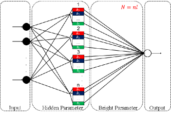
Figure 1: Topological structures of FNN-realization of LtDaHP.

Based on the deterministic assignment of hidden parameters, LtDaHP then transforms a nonlinear optimization problem (2) into a linear one (5), which reduces heavily the computational burden. It should be mentioned that for ESNs, there is another approach to deterministically construct hidden parameters [39]. However, ESNs focus on training recurrent neural networks rather than the standard FNN studied in this paper.

III Theoretical assessment

In this section we study theoretical behaviors of LtDaHP. After reviewing some basic notations of learning theory [9], we prove that the FNN-realization of LtDaHP provides an almost optimal generalization error bound as long as the regression function is smooth.

III-A Statistical Learning Theory

Suppose that $\mathbf{z}=(x_{i},y_{i})_{i=1}^{m}$ are drawn independently and identically from $Z:=X\times Y$ according to an unknown probability distribution $\rho$ which admits the decomposition

$$\rho(x,y)=\rho_{X}(x)\rho(y|x).$$

Assume that $f:X\rightarrow Y$ is a function that characterizes the correspondence between the input and output, as induced by $\rho$. A natural measurement of the error incurred by using $f$ of this purpose is the generalization error, defined by

$$\mathcal{E}(f):=\int_{Z}(f(x)-y)^{2}d\rho,$$

which is minimized by the regression function [9, Chap.1]

$$f_{\rho}(x):=\int_{Y}yd\rho(y|x).$$

We do not know this ideal minimizer $f_{\rho}$ since $\rho$ is unknown, but we have access to random examples ${\bf z}$ from $X\times Y$ sampled according to $\rho$.

Let $L_{\rho_{{}_{X}}}^{2}$ be the Hilbert space of $\rho_{X}$-square-integrable functions on $X$, with norm $\|\cdot\|_{\rho}.$ It is known that, for every $f\in L_{\rho_{X}}^{2}$, there holds [9, Chap.1]

$$\mathcal{E}(f)-\mathcal{E}(f_{\rho})=\|f-f_{\rho}\|_{\rho}^{2}.$$ (6)

So, the goal of learning is to find a best approximation of the regression function $f_{\rho}$.

If we have a specific estimator $f_{\mathbf{z}}$ of $f_{\rho}$ in hand, the error $\mathcal{E}(f_{\mathbf{z}})-\mathcal{E}(f_{\rho})$ clearly depends on $\mathbf{z}$ and therefore has a stochastic nature. As a result, it is impossible to say anything about $\mathcal{E}(f_{\mathbf{z}})-\mathcal{E}(f_{\rho})$ in general for a fixed $\mathbf{z}$. Instead, we can look at its behavior in probability as measured by the following expected error

$$\mathbf{E}_{\rho^{m}}(\|f_{\mathbf{z}}-f_{\rho}\|_{\rho}^{2}):=\int_{Z^{m}}\|f_{\mathbf{z}}-f_{\rho}\|_{\rho}^{2}d\rho^{m},$$

where the expectation is taken over all realizations $\mathbf{z}$ obtained for a fixed $m$, and $\rho^{m}$ is the $m$ fold tensor product of $\rho$.

It is known [47] that whenever $y\in[-M,M],$ using the truncation operator $\pi_{M}$ can reduce the generalization error of $f_{\bf z}$ without adding extra computation. Thus, instead of using $f_{\mathbf{z},\ell,n,\phi}$ defined by (5), we take $\pi_{M}f_{\mathbf{z},\ell,n,\phi}(x)$ as the LtDaHP estimator, where $\pi_{M}f(x):=\mbox{sign}(f(x))\min\{M,|f(x)|\}$ is the truncation operator on $f(x)$.

III-B An Almost Optimal Generalization Bound

In general, it is impossible to get a nontrivial generalization error bound of a learning algorithm without knowing any information on $\rho$ [12, Thm.3.1]. So, some types of a-priori information of the regression function $f_{\rho}$ have to be imposed. Let $\mathbb{N}$ be the set of positive integers and $\mathbf{k}=(k_{1},k_{2},\dots,k_{d})$ with each $k_{i}\in\mathbb{N}.$ The ${\bf k}$-th order derivative of a function $f$ is defined by

$$D^{\mathbf{k}}f(x):=\frac{\partial^{|\mathbf{k}|}f}{\partial^{k_{1}}x^{(1)}\cdots\partial^{k_{d}}x^{(d)}},$$

where $|\mathbf{k}|:=k_{1}+\cdots+k_{d}$ and $x=(x^{(1)},\dots,x^{(d)})$. The classical Sobolev class is then defined for any $r\in\mathbb{N}$ by

$$W_{p}^{r}:=W_{p}^{r}(\mathbb{B}^{d}):=\left\{f:\mathbb{B}^{d}\rightarrow\mathbb{R}^{1}:\max_{0\leq|\mathbf{k}|\leq r}\|D^{\mathbf{k}}f\|_{p}<\infty\right\}.$$

Let $J$ be the identity mapping

$$L^{2}(\mathbb{B}^{d})~{}~{}{\stackrel{{\scriptstyle J}}{{\longrightarrow}}}~{}~{}L^{2}_{\rho_{X}}.$$

and $D_{\rho_{X}}=$ $\|J\|.$ $D_{\rho_{X}}$ is called the distortion of $\rho_{X}$, which measures how much $\rho_{X}$ distorts the Lebesgue measure. We assume that the distribution $\rho$ satisfies $D_{\rho_{X}}<\infty$ and $f_{\rho}\in W_{2}^{r}$, which is standard and utilized in vast literature [12, 9, 32, 43, 23, 26].

Since the generalization capability of LtDaHP depends also on the activation function $\phi,$ certain restrictions on $\phi$ should be imposed. We say that $\phi$ is a sigmoid function, if $\phi$ satisfies

$$\lim_{t\rightarrow\infty}\phi(t)=1,\quad\lim_{t\rightarrow-\infty}\phi(t)=0.$$

By definition, for any sigmoid function $\phi,$ there exists a positive constant $L$ such that

$$\left\{\begin{array}[]{cc}|\phi(u)-1|<m^{-\frac{2}{2r+d}},&\mbox{if}\quad u\geq L,\\ |\phi(u)|<m^{-\frac{2}{2r+d}},&\mbox{if}\quad u\leq-L.\end{array}\right.$$ (7)

Define

$$\phi_{K}(t):=\phi(Kt),$$

for any

$$K\geq\ell L,$$ (8)

where $\ell$ is the number of different thresholds in the LtDaHP scheme. We further suppose that for arbitrary closed set $A$ in $\mathbb{R}^{1},$ $\phi$ is square integrable, which is denoted by $\phi\in L_{Loc}^{2}(\mathbb{R}^{1}).$

Our main result is the following Theorem 1, which shows that $f_{\mathbf{z},\ell,n,\phi_{K}},$ the defined LtDaHP estimator (5), can achieve an almost optimallearning rate.

Theorem 1

Let $d\geq 2$. Assume $0<r\leq\frac{d+1}{2}$, $\phi\in L_{Loc}^{2}(\mathbb{R}^{1})$ is a bounded sigmoid function and $f_{\mathbf{z},\ell,n,\phi_{K}}$ is the LtDaHP estimator defined by (5). If $f_{\rho}\in W_{2}^{r}$, $\ell=\left[m^{\frac{1}{d+2r}}\right]$, $n\sim l^{d-1}$ and $K$ satisfies (8), then there exist positive constants $C_{1}$ and $C_{2}$, depending only on $d,r,M$ and $\phi$, such that,

$$C_{1}m^{-\frac{2r}{d+2r}}\leq\sup_{f_{\rho}\in W_{2}^{r}}\mathbf{E}_{\rho^{m}}(\|f_{\rho}-\pi_{M}f_{\mathbf{z},\ell,n,\phi_{K}}\|_{\rho}^{2})\leq C_{2}D_{\rho_{X}}^{2}m^{-\frac{2r}{d+2r}}\log m.$$ (9)

The proof of Theorem 1 will be presented in Appendix. Some immediate remarks, to explain this result, are as follows.

III-C Remarks

III-C1 On optimality of generalization error

We see that modulo the logarithmic factor $\log m$, the established learning rate (9) is optimal in a minmax sense. That is, up to a logarithmic factor, the upper and lower bounds of the learning rate are asymptotically identical. We further show that this learning rate is also almost optimal among all learning schemes. Let $\mathcal{J}(W_{2}^{r})$ be the class of all Borel measures $\rho$ satisfying $f_{\rho}\in W_{2}^{r}$ and $D_{\rho_{X}}<\infty$. We enter into a competition over all estimators $\mathcal{A}_{m}:\mathbf{z}\rightarrow f_{\mathbf{z}}$ and define

$$e_{m}(W_{2}^{r}):=\inf_{\mathcal{A}_{m}}\sup_{\rho\in\mathcal{J}(W_{2}^{r})}\mathbf{E}_{\rho^{m}}(\|f_{\rho}-f_{\mathbf{z}}\|_{\rho}^{2}).$$

Then, $e_{m}(W_{2}^{r})$ quantitatively measures the quality of $f_{\mathbf{z}}$ and it was shown in [12, Chap. 3] that

$$e_{m}(W_{2}^{r})\geq Cm^{-\frac{2r}{2r+d}},\ m=1,2,\dots,$$ (10)

where $C$ is a constant depending only on $M$, $d$ and $r.$ (10) shows that if $f_{\rho}\in W_{2}^{r}$ and $D_{\rho_{X}}<\infty,$ learning rates of all learning strategies based on $m$ samples cannot be faster than $\mathcal{O(}m^{-\frac{2r}{2r+d}}).$ Consequently, the learning rate established in (9) is almost optimal among all learning schemes.

In this sense, Theorem 1 says that even when the hidden parameters are not trained and just preassigned deterministically, LtDaHP does not degrade the generalization capability of FNNs which train hidden and bright parameters together by some OSL scheme. It is noted that a similar almost optimal learning rate has also been proved in [28] for a typical scheme of LtRaHP (ELM):

$$C_{1}m^{-\frac{2r}{d+2r}}\leq\sup_{f_{\rho}\in W_{2}^{r}}\mathbf{E}_{\mu}\mathbf{E}_{\rho^{m}}(\|f_{\rho}-\pi_{M}f_{LRHP}\|_{\rho}^{2})\leq C_{2}D_{\rho_{X}}^{2}m^{-\frac{2r}{d+2r}}\log m,$$ (11)

in which the expectation $\mathbf{E}_{\mu}$ is taken over all possible random assignments of hidden parameters. We refer the readers to [28] for detailed definitions of $f_{LRHP}$ and $\mu$. There is an additional expectation term that brings the uncertainty problem of LtRaHP. Comparing (11) with (9), we can see that the LtDaHP dismisses the $\mathbf{E}_{\mu}$-expectation term. Furthermore, we notice that LtRaHP, as shown in [24], may break the almost optimal generalization error for certain specific activation functions even in the $\mathbf{E}_{\mu}$-expectation sense. Theorem 1 thus implies that the LtDaHP improves on LtRaHP not only in circumventing the uncertainty problem, but also guaranteeing the generalization capability further.

III-C2 On how to specify the activation function $\phi$

In Theorem 1, three conditions have been imposed on the activation function $\phi:\$(i) $\phi_{K}(t)=\phi(Kt)$ with $K\geq\ell L$, where $L$ is defined by (7),  (ii) $\phi$ is a bounded sigmoid function, and $(iii)$ $\phi\in L_{Loc}^{2}(\mathbb{R}^{1}).$ The conditions (ii) and (iii) are clearly mild, say, both the widely applied heaviside function $\sigma_{H}$ and logistic function $\sigma_{L}$ satisfy the assumptions, where

$$\sigma_{H}(t):=\left\{\begin{array}[]{cc}1,&t\geq 0\\ 0,&t<0\end{array}\right.$$

and

$$\sigma_{L}(t)=\frac{1}{1+e^{-t}}.$$

The most crucial assumption is (i), i.e., $K$ should be carefully chosen. It is observed that $K$ in (8) is with respective to $\ell$ and $L$, while $L$ depends merely on $m$ and $\phi.$ So $K$ can be specified when $\phi$ is given. For example, if $\phi$ is the logistic function, then $K$ can be selected as any positive numbers satisfying $K\geq\ell\log(\ell^{2}-1)$.

The problem is that there are infinite many choices of such $K$. How to specify the best $K$ thus becomes a practical issue. According to [31, Thm. 2.4], the complexity of $\mathcal{H}_{{\ell,n,\phi_{K}}}$ monotonously increases with respect to $K$. Due to the well known bias and variance trade-off principle, we then recommend to choose $K=\ell L$ in practice. For example, when the logistic function is utilized, we may take $K=\ell\log(\ell^{2}-1)$ if $\ell\geq 2,$ and $K=\log 2$ if $\ell=1$.

III-C3 On almost optimality of the number of hidden neurons

Theorem 1 has presented the number of hidden neurons to be $n\ell=\mathcal{O}(m^{\frac{d}{2r+d}}).$ We observe from (4) that $\mathcal{H}_{\ell,n,\phi_{K}}$ is an $n\ell$-dimensional linear space. Hence, according to the well known linear width theory [38], for $f_{\rho}\in W_{2}^{r}$, $n\ell$ must be not smaller than $\mathcal{O}(m^{\frac{d}{2r+d}})$ if one wants to achieve an approximation error of $\mathcal{O}(m^{\frac{-2r}{2r+d}}).$ This means that the number of hidden neurons required in Theorem 1 cannot be reduced.

At the first glance, there are two parameters, $\ell$ and $n$, that need to be specified, which is more complicated than that in OSL [32] and LtRaHP [28]. In fact, there is only an essential parameter since $n$ and $\ell$ have a relation $n\sim\ell^{d-1}$. If the smoothness information of $f_{\rho}$ is known, one can directly take $n\sim\ell^{d-1}=\left[m^{\frac{1}{d+2r}}\right]^{d-1}$ as that in Theorem 1. However, it is usually infeasible since we do not know the concrete value of $r$, when faced with real world applications. Instead, we turn to some model-selection strategy such as the “cross-validation” approach [12, Chap.8] to determine $\ell$ and $N$.

III-C4 On why LtDaHP works

It is known [9, Chap.1] that a satisfactory generalization capability of a learning scheme can only be resulted from an appropriate trade-off between the approximation capability and capacity of the hypothesis space. We use this principle to explain the success of LtDaHP.

Given a hypothesis space $\mathcal{F}$ and a function $f,$ the approximation capability of $\mathcal{F}$ can be measured by its best approximation error:$dist(f,\mathcal{F}):=\inf_{g\in\mathcal{F}}\|f-g\|_{2}$ while the capacity of $\mathcal{F}$ can be measured by its pseudo-dimension [31], denoted by $Pdim(\mathcal{F})$. We compare the approximation capabilities and capacities of the hypothesis spaces of FNNs and LtDaHP. The hypothesis space $\mathcal{N}_{N,K}^{\ast}$ of FNNs is the family of functions of the form

$$N_{N,K}(x):=\sum_{j=1}^{N}c_{j}\phi(\alpha_{j}\cdot x-b_{j})$$

where $\|\alpha_{j}\|\leq K$ and $|b_{j}|\leq K$. In [31] and [27], it was shown that for some positive constant $c$ there holds

$$Pdim(\mathcal{N}_{N,K}^{\ast})\leq cd^{2}N\log(KN),$$ (12)

if $\phi$ is the logistic function. Furthermore, in [32], it was verified the approximation capability of $\mathcal{N}_{N,K}^{\ast}$ satisfies

$$dist(f,\mathcal{N}_{N,K}^{\ast})\leq CN^{-r/d}.$$ (13)

provided $f_{\rho}\in W_{2}^{r}.$

In comparison, we find in [34] that

$$Pdim(\mathcal{H}_{{\ell,n,\phi_{K}}})=N$$ (14)

and, similarly, we can prove in Lemma 6 that

$$dist(f,\mathcal{H}_{\ell,n,\phi_{K}})\leq c(n\ell)^{-r/d}=cN^{-r/d},$$ (15)

as long as $K$ satisfies (8). Comparing (12) and (13) with (14) and (15), we thus conclude that for appropriately tuned $K$, both the approximation capabilities and capacities of $\mathcal{N}_{N,K}^{\ast}$ and $\mathcal{H}_{l,n,\phi_{K}}$ are almost the same. This shows the reason why the LtDaHP scheme performs at least not worse than the conventional FNNs.

IV Experimental Studies

In this section, we present both toy simulations and real world data experiments to assess the performance of LtDaHP as compared with support vector regression (SVR), Gaussian process regression (GPR), and a typical LtRaHP scheme (ELM), where the learning algorithm is the same as LtDaHP, except that the inner weights and thresholds are randomly sampled according to the uniform distribution. In our experiments, the minimal Riesz energy points were approximately generated by the recursive zonal sphere partitioning [22] using the EQSP tool box. SVR and GPR were realized by the Matlab functions fitrsvm and fitrgp(with subsampling 1000 atoms), respectively. For fair of comparisons, we applied the 10-fold cross-validation method [12, Chap.8] to select all parameters (more specifically, to select three parameters in SVR, the width of Gaussian kernel, the regularization parameter and the epsilon-insensitive band, and two parameters in LtRaHP and LtDaHP, the number of hidden neurons for both methods, $\ell$ for LtDaHP, and $K$ for LtRaHP), and the time for parameter tuning was included in recording the training time.

All the simulations and experiments were conducted in Matlab R2017b on a workstation with 64Gb RAM and E5-2667 v2 3.30GHz CPU.

IV-A Toy Simulations

This series of simulations were designed to support the correctness of Theorem 1 and compare the learning performance among LtDaHP, LtRaHP, GPR, and SVR. For this purpose, the regression function $f_{\rho}$ is supposed to be known and given by

$$f_{\rho}(x)=(1-\|x\|_{2})_{+}^{4}(4\|x\|_{2}+1),x\in[-1,1]^{3}$$

where $a_{+}=\max\{a,0\}.$ Direct computation shows $f_{\rho}\in W_{2}^{2}$ and $f_{\rho}\notin W_{2}^{3}$. We generated the training sample set ${\bf z}=\{(x_{i},y_{i})\}_{i=1}^{m}$ with variable data size through independently and randomly sampling $x_{i}$ from $[-1,1]^{3}$ according to the uniform distribution, and $y_{i}=f_{\rho}(x_{i})+\epsilon$ with $\varepsilon\sim N(0,0.1)$ being the white noise. The learning performance of the algorithms were tested by applying the resultant estimators to the test set ${\bf z}_{test}=\{(x_{i}^{(t)},y_{i}^{(t)})\}_{i=1}^{1000}$ which was generated similarly to ${\bf z}$ with a difference that $y_{i}^{(t)}=f_{\rho}(x_{i}^{(t)}).$ In simulations, we took $\phi(t)=\frac{1}{1+e^{-t}},$ and implemented the LtDaHP and LtRaHP with $\phi_{K}(t)=\phi(Kt),$ where

$$K=\left\{\begin{array}[]{cc}\ell\log(\ell^{2}-1),&\ell>1\\ \log 2,&\ell=1\end{array}\right.$$

for LtDaHP as suggested in the subsection III.C. The $\ell$ for LtDaHP and $K$ for LtRaHP were tuned by 10-fold cross validation. In addition, to avoid the risk of singularity, we implement the least square (2) for LtDaHP and LtRaHP with a very small and fixed regularization pamameter $\lambda=10^{-4}$.

In the first simulation, to illustrate the difference between LtDaHP and LtRaHP, we conducted a phase diagram study. To this end, the number of samples $m$ varied from $20$ to $2000$ and the number of neurons $N$ ranged from $5$ to $500$. For each pair $(m,N)$, we implemented 100 independent simulations with LtDaHP and LtRaHP. The average rooted mean square errors (RMSE) were then recorded. We plotted all the simulation results in a figure, called the phase diagram, with $x$-axis and $y$-axis being respectively the number of neurons and the number of samples, and the colors from blue to red corresponding to the RMSE values from small to large. The simulation results are reported in Fig. 2.

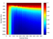
(a) LtDaHP phase diagram

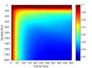
(b) LtRaHP phase diagram

Figure 2: The comparison of generalization capability between LtDaHP and LtRaHP

Fig. 2(a) shows that for suitable choice of $N$, the LtDaHP estimator maintains always very low RMSE, which coincides with Theorem 1. Furthermore, comparing (a) with (b) in Fig. 2 demonstrates several obvious differences between LtDaHP and LtRaHP: (i) the test errors of LtDaHP are much smaller than those of LtRaHP. This can be observed not only for the best choice of the number of neurons, but also for every fixed number of neurons as well. This difference reveals that as far as the generalization capability is concerned, LtDaHP outperforms LtRaHP in this example.  (ii) LtDaHP exhibits a somewhat tidy phase change phenomenon: there is a clear range of $m$ and $N$ such that the LtDaHP performs well. Similar phase change phenomenon does not appear in LtRaHP, as exhibited in Fig. 2(b), due to the uncertainty. This difference implies that LtDaHP is more robust to the specification of neuron number $N$ than LtRaHP and selecting an appropriate neuron number $N$ for LtDaHP is much easier than that for LtRaHP. All these differences show the advantages of LtDaHP over LtRaHP.

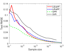
(a) Comparison of test error

(b) Comparison of training time

(c) Comparison of model sparsity

Figure 3: The comparisons of test error, training time, and model sparsity among LtDaHP, LtRaHP, GPR, and SVR.

In the second simulation, we studied the pros and cons of LtDaHP, LtRaHP, GPR, and SVR. We implemented these four algorithms independently 50 times and calculated the average RMSEs. The obtained RMSEs, as well as the corresponding computational time and model sparsity, were plotted as a function of the number of training samples in Fig. 3.

From Fig. 3(a), we can see that GPR performs with the best generalization capability, then LtDaHP, LtRaHP and finally SVR. More specifically, we observe that the test errors of LtDaHP are very close to GPR when the sample size is over $1000$. But LtRaHP requires more samples to reach comparable performances. From Fig. 3(b) we can see that LtDaHP and LtRaHP have constantly low training time. In this simulation, GPR has lower training time when samples are smaller than $10000$, but is less predictable due to more complex algorithm. In addition, SVR always takes more time for training, since there are 3 hyper-parameters to be tuned. Finally from Fig. 3(c) we can see that LtDaHP and LtRaHP has much smaller model sparsity than SVR, which suggests less time in prediction.

All these simulations support the outperformance of LtDaHP and the theoretical assertions made in the previous sections.

IV-B Real World Benchmark Data Experiments

Data sets	Training samples	Testing samplesr	Attributes
Machine	167	42	7
Yacht	246	62	6
Energy	614	154	8
Stock	760	190	9
Concrete	824	206	8
Bank8FM	3599	900	8
Delta_ailerons	5703	1426	5
Delta_elevators	7613	1904	6
Elevator	13279	3320	18
Bike	13903	3476	17

TABLE I: Setting-up for data sets

Data set	TestRMSE				TrainMT				MSparsity
	LtDaHP	LtRaHP	GPR	SVR	LtDaHP	LtRaHP	GPR	SVR	LtDaHP	LtRaHP	SVR
Machine	$0.084\pm 0.011$	$0.081\pm 0.013$	$0.082\pm 0.013$	$0.105\pm 0.019$	1.8	0.3	0.1	2.6	51.8	45.4	145.7
Yacht	$0.012\pm 0.007$	$0.027\pm 0.009$	$0.012\pm 0.006$	$0.049\pm 0.018$	1.9	0.5	0.1	3.0	131.8	123.6	165
Energy	$0.015\pm 0.003$	$0.053\pm 0.005$	$0.012\pm 0.001$	$0.019\pm 0.002$	3.5	0.8	1.6	6.5	195	190	439
Stock	$0.039\pm 0.003$	$0.039\pm 0.003$	$0.038\pm 0.003$	$0.054\pm 0.009$	3.3	0.45	0.24	5.1	76	106	377
Concrete	$0.072\pm 0.005$	$0.079\pm 0.006$	$0.068\pm 0.006$	$0.072\pm 0.007$	4.1	0.8	0.9	9.2	204	211	606
Bank8FM	$0.040\pm 0.001$	$0.040\pm 0.001$	$0.037\pm 0.001$	$0.039\pm 0.002$	13	9	8	222	335	439	1938
Delta_a	$0.038\pm 0.001$	$0.038\pm 0.001$	$0.039\pm 0.001$	$0.040\pm 0.002$	16	14	8	222	534	497	2617
Delta_e	$0.053\pm 0.001$	$0.053\pm 0.001$	$0.053\pm 0.001$	$0.053\pm 0.001$	25	22	9	357	482	534	3564
Elevator	$0.052\pm 0.001$	$0.052\pm 0.001$	$0.052\pm 0.001$	$0.054\pm 0.001$	55	51	353	703	768	730	5455
Bike	$0.032\pm 0.001$	$0.064\pm 0.002$	$0.049\pm 0.001$	$0.052\pm 0.002$	57	51	389	660	792	792	3764

TABLE II: Results of SVR, LtRaHP and LtDaHP when applied to the 10 real world benchmark data sets

We further apply LtDaHP, LtRaHP, GPR, and SVR to a family of real world benchmark data sets. We include 10 problems covering different fields. With the training and testing samples drawn as in Table 1, we used 10-fold cross-validation to select all the parameters involved in each algorithm. Then we implemented each algorithm independently 50 times and calculated the rooted mean square error (TestRMSE) of the estimator. It was also recorded the corresponding average training time (TrainMT) for each algorithm. For comparison of testing complexity, we recorded the average number of hidden neurons (MSparsity) involved in LtDaHP, LtRaHP, and SVR. The simulation results are listed in Table II.

We can see from Table II that LtDaHP works well for most of the data sets, exhibiting an almost similar or comparable generalization performance to GPR. Both LtRaHP and SVR failed in certain data sets.

As far as the training time and testing complexity are concerned, LtDaHP and LtRaHP significantly outperform SVR, and are better than GPR when sample size is higher than 10000. Furthermore, we can observe that LtDaHP and LtRaHP always keep a similar training time and testing complexity.

IV-C Real World Massive Data Experiments

In this section we assess the performance of LtDaHP and LtRaHP through applying the algorithms to a real world massive data.

The problem we have applied is the household electric power consumption data set. The task is to predict the global active power from $8$ primary features. The dataset contains $2075259$ samples, and so a real large scale problem. We applied LtDaHP and LtRaHP to this problem by dividing the sample dataset into a training set containing $90\%$ samples and a test set containing $10\%$ samples. 10 random partitions of the data were implemented and the results were recorded in Table III. Under such an experimental setting, the RMSE predicted by GPR is $0.053\pm 0.000$, while the deep kernel machine(DKL) can achieve $0.048\pm 0.000$, as reported in [11].

We only compare the performance of LtDaHP and LtRaHP because of the extremely high computational burden of SVR for such a large scale problem. Both algorithms were applied with neuron number $N$ varying from $400$ to $30000$. We plot the obtained RMSEs of test error as a function of $N$ to demonstrate the performances of LtDaHP and LtRaHP in Fig. 4. Fig. 4 shows that for most choices of $N$, LtDaHP performs much better than LtRaHP.

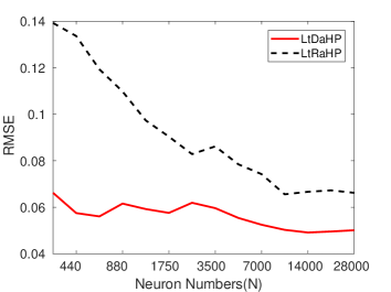
Figure 4: The comparisons of test error of household electricity data between LtDaHP and LtRaHP.

To compare the performance of LtDaHP and LtRaHP further, we implemented the algorithms in which the parameters were chosen by using the 5-fold cross-validation method. The resultant RMSEs, TrainMT, and Msparsity are shown in Table III.

Methods	TestRMSE	TrainMT	Msparsity
LtDaHP	$0.049\pm 0.000$	57330s	14032
LtRaHP	$0.065\pm 0.001$	57610s	14032

TABLE III: Comparison of LtDaHP and LtRaHP on the house electric dataset

From Table III we see that LtDaHP performs much better than LtRaHP with respect to the TestRMSE, and they achieve a similar training time and model sparsity. In addition, LtDaHP achieves comparable result to DKL, and slightly better than GPR. But it should be noted that both DKL and GPR are lack of theoretical guarantees. However, both LtDaHP and LtRaHP cost more computation time than DKL(which is 3600s as reported in [11]) due to an additional procedure of parameter tuning. We believe that with some other additional precision-promoting skills used, like “divide and conquer” in [25, 5], the performance of LtDaHP can be further improved.

All these simulations and experiments support that, as a new TSL scheme, LtDaHP outperforms LtRaHP in generalization capability and SVR in computational complexity. It is also comparable with GPR in numerical ability but possesses almost optimal theoretical guarantees.

V Conclusions

In this paper, we proposed a new TSL scheme: learning through deterministic assignment of hidden parameters (LtDaHP). The main contributions can be concluded as follows:

• Borrowing an approximate solution to the classical Tamme’s problem, we suggested to set inner weights of FNNs as minimal Riesz $\tau$-energy points on the sphere and thresholds as equally spaced points in an interval;

• We proved that with the suggested deterministic assignment mechanism of the hidden parameters, LtDaHP achieves an almost optimal generalization bound (learning rate). In particular, it does not degrade the generalization capability of the classical one-stage learning schemes very much.

• A series of simulations and application examples were provided to support the correctness of the theoretical assertions and the effectiveness of the LtDaHP scheme.

Additionally, we found that the outperformance of LtDaHP over LtRaHP demonstrated in the house electric prediction problem in Section V.C shows that LtDaHP may be more effectively applied to practical problems, especially for large scaled problems. We finish this section with two additional remarks.

Remark 1

It should be remarked that LtDaHP involves an adjustable parameter $K$ that may have a crucial impact for its performance. We have suggested a criterion of specification of $K$ for the logistic function, and the simulations in Section 4 have substantiated the validity and effectiveness of such a criterion. This criterion is, however, by no means universal. In other words, it is perhaps inadequate for other activation functions. Thus, how to generally set an appropriate K in implementation of LtDaHP is still open. We leave it for our future study.

Remark 2

The minimal Riesz energy points were approximated by the recursive zonal sphere partitioning. However, the EQSP algorithm is not robust in high-dimensional cases, which makes the corresponding LtDaHP scheme instably training high dimensional data. We will work on data-driven methods by taking the sample distribution to determine the hidden parameters in a future work.

Appendix:Proof of Theorem 1

We divide the proof of Theorem 1 into five parts. The first part concerns the orthonormal system in $L^{2}(\mathbb{B}^{d})$. The second part focuses on the ridge representations for polynomials. The third one aims at constructing an FNN in $\mathcal{H}_{\ell,n,\phi_{K}}$, while the fourth part pursues its approximation ability. In the last part, we analyze the learning rate of (5).

V-A Orthonormal basis for multivariate polynomials on the unit ball

Let $G_{s}^{\nu}(t)$ be the Gegenbauer polynomial [46] with index $\nu$. It is known that the family of polynomials $\{G_{s}^{\nu}\}_{s=0}^{\infty}$ is a complete orthogonal system in the weighted space $L^{2}(\mathbb{I},w_{\nu})$ with $\mathbb{I}:=[-1,1]$ and $w_{\nu}(t):=(1-t^{2})^{\nu-\frac{1}{2}}$, that is,

$$\int_{\mathbb{I}}G_{s^{\prime}}^{\nu}(t)G_{s}^{\nu}(t)w_{\nu}(t)dt=\left\{\begin{array}[]{cc}0,&s^{\prime}\neq s\\ h_{s,\nu},&s^{\prime}=s\end{array}\right.,$$

where $h_{s,\nu}=\frac{\pi^{1/2}(2\nu)_{s}\Gamma(\nu+\frac{1}{2})}{(s+\nu)s!\Gamma(\nu)},$ and

$$(a)_{0}:=0,(a)_{s}:=a(a+1)\dots(a+s-1)=\frac{\Gamma(a+s)}{\Gamma(a)}.$$

Define

$$U_{s}:=(h_{s,d/2})^{-1/2}G_{s}^{d/2},\ s=0,1,\dots.$$ (16)

Then, $\{U_{s}\}_{s=0}^{\infty}$ is a complete orthonormal system for the weighted space $L^{2}(\mathbb{I},w)$ with $w(t):=(1-t^{2})^{\frac{d-1}{2}}$. With this, we introduce the univariate Sobolev spaces

$$W^{\alpha}(L^{2}(\mathbb{I},w)):=\left\{g:\|g\|^{2}_{W^{\alpha}(L^{2}(\mathbb{I},w))}=\sum_{k=0}^{\infty}\left[(k+1)^{\alpha}\hat{g}_{w,k}\right]^{2}<\infty\right\},$$

where $\hat{g}_{w,k}:=\int_{\mathbb{I}}g(t)U_{k}(t)w(t)dt.$ It is easy to see that

$$\|p\|_{W^{\alpha}(L^{2}(\mathbb{I},w))}\leq(s+1)^{\alpha}\|p\|_{L^{2}(\mathbb{I},w)},\qquad\forall\ p\in\mathcal{P}_{s}(\mathbb{I}),$$ (17)

where $\mathcal{P}_{s}(\mathbb{I})$ denotes the algebraic polynomials defined on $\mathbb{I}$ of degrees at most $s$.

Denote by $\mathbb{H}^{d-1}_{j}$ and $\Pi_{s}^{d-1}$ the class of all spherical harmonics of degree $j$ and the class of all spherical polynomials with total degrees $j\leq s$, respectively. It can be found in [46] that $\Pi_{s}^{d-1}=\bigoplus_{j=0}^{s}\mathbb{H}^{d-1}_{j}$. Since the dimension of $\mathbb{H}^{d-1}_{j}$ is given by

$$D_{j}^{d-1}:=\mbox{dim }\mathbb{H}^{d-1}_{j}=\left\{\begin{array}[]{ll}\frac{2j+d-2}{j+d-2}{{j+d-2}\choose{j}},&j\geq 1;\\ 1,&j=0,\end{array}\right.$$

the dimension of $\Pi_{s}^{d-1}$ is $\sum_{j=0}^{s}D^{d-1}_{j}=D_{s}^{d}\sim s^{d-1}.$ Let $\{Y_{j,i}:i=1,\dots,D_{j}^{d-1}\}$ be an arbitrary orthonormal system of $\mathbb{H}_{j}^{d-1}$. The well known addition formula is given by [46]

$$\sum_{i=1}^{D_{j}^{d-1}}Y_{j,i}(\xi)Y_{j,i}(\eta)=\frac{2j+d-2}{(d-2)\Omega_{d-1}}G_{j}^{\frac{d-2}{2}}(\xi\cdot\eta)=K_{j}^{*}(\xi\cdot\eta),$$ (18)

where $K_{n}^{*}(t):=\frac{2j+d-2}{(d-2)\Omega_{d-1}}G_{j}^{\frac{d-2}{2}}(t)$, $\Omega_{d-1}:=\int_{\mathbb{S}^{d-1}}d\omega_{d-1}=\frac{2\pi^{\frac{d}{2}}}{\Gamma(\frac{d}{2})},$ and $d\omega_{d-1}$ denotes the aero element of $\mathbb{S}^{d-1}$

For $x\in\mathbb{B}^{d}$, define

$$P_{k,j,i}(x)=v_{k}\int_{\mathbb{S}^{d-1}}Y_{j,i}(\xi)U_{k}(x\cdot\xi)d\omega_{d-1}(\xi),$$ (19)

where $v_{k}:=\left(\frac{(k+1)_{d-1}}{2(2\pi)^{d-1}}\right)^{\frac{1}{2}}$. Then it follows from [33] that

$$\{P_{k,j,i}:k=0,1,\dots,s,j=k,k-2,\dots,\varepsilon_{k},i=1,2,\dots,D_{j}^{d-1}\}$$

is an orthonormal basis for $\mathcal{P}_{s}(\mathbb{B}^{d})$ with $\varepsilon_{k}:=\left\{\begin{array}[]{cc}0,&k\ \mbox{even},\\ 1,&k\ \mbox{odd}\end{array}\right..$ Based on the orthonormal system, we define the Sobolev space on $\mathbb{B}^{d}$, denoted by $H^{r}(L^{2}(\mathbb{B}^{d}))$, as the space

$$\left\{f:\|f\|^{2}_{H^{r}(L^{2}(\mathbb{B}))}=\sum_{k=0}^{\infty}\sum_{j\in\Xi_{k}}\sum_{i=1}^{D_{j}^{d-1}}\left[(k+1)^{r}\hat{f}_{k,j,i}\right]^{2}<\infty\right\},$$

where $\hat{f}_{k,j,i}:=\int_{\mathbb{I}}f(x)P_{k,j,i}(x)dx$ and $\Xi_{k}:=\{k,k-2,\dots,\varepsilon_{k}\}$.

V-B Ridge function representation for multivariate polynomials on the ball

For $s\geq 0$ and $N\geq 1$, let a discretization quadrature rule

$$\mathcal{Q}_{N}(s,n):=\{(\lambda_{\ell},\xi_{\ell}):\ell=1,\dots,n\},\quad\lambda_{\ell}>0$$ (20)

holds exact for $\Pi_{s}^{d-1}$. By the sequence of works in [20, 21], we find that all minimal $\tau$-energy configurations with $\tau\geq d$ is a discretization quadrature rule $\mathcal{Q}_{N}(2s,n)$. The following positive cubature formula can be found in [2].

Lemma 1

If $\tau\geq d$, then there exists a set of numbers $\{\lambda_{z}\}_{z\in\mathcal{E}_{\tau}(\mathbb{S}^{d-1},n)}$ such that

$$\int_{\mathbb{S}^{d-1}}P(y)d\omega(y)=\Omega_{d-1}\sum_{z\in\mathcal{E}_{\tau}(\mathbb{S}^{d-1},n)}\lambda_{z}P(z)\ \ \mbox{for}\ \mbox{any \ \ }P\in\Pi_{2s}^{d-1}.$$

We then present the main tool for our analysis in the following proposition.

Proposition 1

Let $s\in\mathbb{N}$. If $\mathcal{Q}_{N}(2s,n)=\{\lambda_{\ell},\xi_{\ell}\}_{\ell=1}^{n}$ is a discretization quadrature rule for spherical polynomials of degree up to $2s$, then for arbitrary $P\in\mathcal{P}_{s}(\mathbb{B}^{d})$, there holds

$$P(x)=\sum_{\ell=1}^{n}\lambda_{\ell}p_{\ell}(\xi_{\ell}\cdot x),$$ (21)

and

$$\sum_{\ell=1}^{n}\lambda_{\ell}\|p_{\ell}\|^{2}_{W^{1}(L^{2}(\mathbb{I},w))}\leq c_{3}\|P\|^{2}_{H^{\frac{d+1}{2}}(L^{2}(\mathbb{B}^{d}))},$$ (22)

where

$$p_{\ell}(t):=\sum_{k=0}^{s}v_{k}^{2}\int_{\mathbb{B}^{d}}U_{k}(\xi_{\ell}\cdot y)P(y)dyU_{k}(t)$$ (23)

and $c_{3}$ is a constant depending only on $d$.

We postpone the proof of Proposition 1 to the end of this subsection and introduce the following lemma concerning important properties of $U_{s}$ at first.

Lemma 2

Let $U_{s}$ be defined as above. Then for each $\xi,\eta\in\mathbb{S}^{d-1}$ we have

$$\int_{\mathbb{B}^{d}}U_{s}(\xi\cdot x)P(x)dx=0\ \mbox{for}\ P\in\mathcal{P}_{s-1}(\mathbb{B}^{d}),$$ (24)

$$\int_{\mathbb{B}^{d}}U_{s}(\xi\cdot x)U_{s}(\eta\cdot x)dx=\frac{U_{s}(\xi\cdot\eta)}{U_{s}(1)},$$ (25)

$$K_{s}^{*}+K_{s-2}^{*}+\dots+K_{\varepsilon_{s}}^{*}=\frac{v_{s}^{2}}{U_{s}(1)}U_{s},$$ (26)

$$\int_{\mathbb{S}^{d-1}}U_{s}(\xi\cdot x)U_{s}(\xi\cdot\eta)d\omega_{d-1}(\xi)=\frac{U_{s}(1)}{v_{s}^{2}}U_{s}(\eta\cdot x),$$ (27)

and

$$\int_{\mathbb{S}^{d-1}}U_{k}(\xi\cdot x)U_{k}(\xi\cdot y)d\omega_{d-1}(\xi)=\frac{1}{v_{k}^{2}}\sum_{j\in\Xi_{k}}\sum_{i=1}^{D_{j}^{d-1}}P_{k,j,i}(x)P_{k,j,i}(y).$$ (28)

Proof:

(24)-(27) can be found in eqs. (3.4), (3.10), (3.16), (3.11) of [37], respectively. It suffices to prove (28). We get from (19) that

$$\sum_{j\in\Xi_{k}}\sum_{i=1}^{D_{j}^{d-1}}P_{k,j,i}(x)P_{k,j,i}(y)$$

$$= \sum_{j\in\Xi_{k}}\sum_{i=1}^{D_{j}^{d-1}}v_{k}^{2}\int_{\mathbb{S}^{d-1}}Y_{j,i}(\xi)U_{k}(x\cdot\xi)d\omega_{d-1}(\xi)$$

$$\int_{\mathbb{S}^{d-1}}Y_{j,i}(\eta)U_{k}(y\cdot\eta)d\omega_{d-1}(\eta)$$

$$= v_{k}^{2}\sum_{j\in\Xi_{k}}\int_{\mathbb{S}^{d-1}}U_{k}(x\cdot\xi)\int_{\mathbb{S}^{d-1}}U_{k}(y\cdot\eta)$$

$$\times \sum_{i=1}^{D_{j}^{d-1}}Y_{j,i}(\xi)Y_{j,i}(\eta)d\omega_{d-1}(\xi)d\omega_{d-1}(\eta).$$

Thus, the addition formula (18) yields

$$\sum_{j\in\Xi_{k}}\sum_{i=1}^{D_{j}^{d-1}}P_{k,j,i}(x)P_{k,j,i}(y)=v_{k}^{2}\sum_{j\in\Xi_{k}}\int_{\mathbb{S}^{d-1}}$$

$$\times U_{k}(x\cdot\xi)\int_{\mathbb{S}^{d-1}}U_{k}(y\cdot\eta)K^{*}_{j}(\xi\cdot\eta)d\omega_{d-1}(\xi)d\omega_{d-1}(\eta).$$

The above equality together with (26) and (27) implies

$$\sum_{j\in\Xi_{k}}\sum_{i=1}^{D_{j}^{d-1}}P_{k,j,i}(x)P_{k,j,i}(y)=v_{k}^{2}\int_{\mathbb{S}^{d-1}}U_{k}(x\cdot\xi)$$

$$\times \int_{\mathbb{S}^{d-1}}U_{k}(y\cdot\eta)\sum_{j\in\Xi_{k}}K_{j}^{*}(\xi\cdot\eta)d\omega_{d-1}(\xi)d\omega_{d-1}(\eta)$$

$$= \frac{v_{k}^{4}}{U_{k}(1)}\int_{\mathbb{S}^{d-1}}U_{k}(x\cdot\xi)$$

$$\times \int_{\mathbb{S}^{d-1}}U_{k}(y\cdot\eta)U_{k}(\xi\cdot\eta)d\omega_{d-1}(\xi)d\omega_{d-1}(\eta)$$

$$= v_{k}^{2}\int_{\mathbb{S}^{d-1}}U_{k}(\xi\cdot x)U_{k}(\xi\cdot y)d\omega_{d-1}(\xi).$$

This competes the proof of Lemma 2. ∎

Based on (28) and the well known Aronszajn Theorem, it is easy to construct a reproducing kernel of $\mathcal{P}_{s}(\mathbb{B}^{d})$.

Lemma 3

The space $(\mathcal{P}_{s}(\mathbb{B}^{d}),\langle\cdot,\cdot\rangle_{L^{2}(\mathbb{B}^{d})})$ is a reproducing kernel Hilbert space with the reproducing kernel

$$K_{s}(x,y):=\sum_{k=0}^{s}v_{k}^{2}\int_{\mathbb{S}^{d-1}}U_{k}(\xi\cdot x)U_{k}(\xi\cdot y)d\omega_{d-1}(\xi).$$ (29)

By the help of these lemmas, we are in a position to prove Proposition 1.

Proof:

Due to Lemma 3, for arbitrary $P\in\mathcal{P}_{s}(\mathbb{B}^{d})$, there holds

$$P_{s}(x)=\int_{\mathbb{B}^{d}}K_{s}(x,y)P_{s}(y)dy$$

$$= \int_{\mathbb{B}^{d}}\sum_{k=0}^{s}v_{k}^{2}\int_{\mathbb{S}^{d-1}}U_{k}(\xi\cdot x)U_{k}(\xi\cdot y)d\omega_{d-1}(\xi)P_{s}(y)dy.$$

Since $\mathcal{Q}_{N}(2s,N)=\{\lambda_{\ell},\xi_{\ell}\}_{\ell=1}^{N}$ is a discretization quadrature rule for spherical polynomials of degree up to $2s$, we have

$$P_{s}(x)=\sum_{k=0}^{s}v_{k}^{2}\sum_{\ell=1}^{N}\lambda_{\ell}\int_{\mathbb{B}^{d}}U_{k}(\xi_{\ell}\cdot y)P_{s}(y)dyU_{k}(\xi_{\ell}\cdot x).$$

This proves (21). To derive (22), we use (23), (28) and $v_{k}\leq c_{3}k^{\frac{d-1}{2}}$ for some $c_{3}\geq 1$ and obtain

$$\sum_{\ell=1}^{N}\lambda_{\ell}\|p_{\ell}\|^{2}_{W^{1}(L^{2}(\mathbb{I},w))}$$

$$= \sum_{k=0}^{\infty}(k+1)^{2}\sum_{\ell=1}^{N}\lambda_{\ell}\left(\int_{\mathbb{I}}p_{\ell}(t)U_{k}(t)w(t)dt\right)^{2}$$

$$= \sum_{k=0}^{\infty}(k+1)^{2}\sum_{\ell=1}^{N}\lambda_{\ell}$$

$$\times \left(\int_{\mathbb{I}}\sum_{k^{\prime}=0}^{s}v_{k^{\prime}}^{2}\int_{\mathbb{B}^{d}}U_{k^{\prime}}(\xi_{\ell}\cdot y)P(y)dyU_{k^{\prime}}(t)U_{k}(t)w(t)dt\right)^{2}$$

$$= \sum_{k=0}^{s}(k+1)^{2}\sum_{\ell=1}^{N}\lambda_{\ell}\left(v_{k}^{2}\int_{\mathbb{B}^{d}}U_{k}(\xi_{\ell}\cdot y)P(y)dy\right)^{2}$$

$$= \sum_{k=0}^{s}(k+1)^{2}v_{k}^{4}\sum_{\ell=1}^{N}\lambda_{\ell}\int_{\mathbb{B}^{d}}P(y)$$

$$\int_{\mathbb{B}^{d}}P(z)U_{k}(\xi_{\ell}\cdot y)U_{k}(\xi_{\ell}\cdot z)dydz$$

$$= \sum_{k=0}^{s}(k+1)^{2}v_{k}^{4}\int_{\mathbb{B}^{d}}P(y)\int_{\mathbb{B}^{d}}P(z)$$

$$\int_{\mathbb{S}^{d-1}}U_{k}(\xi\cdot y)U_{k}(\xi\cdot z)d\omega_{d-1}(\xi)dydz$$

$$= \sum_{k=0}^{s}(k+1)^{2}v_{k}^{2}\sum_{j\in\Xi_{k}}\sum_{i=1}^{D_{k}^{d-1}}\int_{\mathbb{B}^{d}}P(y)P_{k,j,i}(y)dy\int_{\mathbb{B}^{d}}P(z)P_{k,j,i}(z)dz$$

$$\leq c_{3}\sum_{k=0}^{s}(k+1)^{d+1}\sum_{j\in\Xi_{k}}\sum_{i=1}^{D_{k}^{d-1}}\hat{P}_{k,j,i}=c_{3}\|P_{s}\|_{H^{\frac{d+1}{2}}(L^{2}(\mathbb{B}^{d}))}^{2}.$$

This completes the proof of Proposition 1. ∎

V-C Constructing neural networks

Before constructing the neural networks, we at first present a univariate Jackson-type error estimate for FNNs with sigmoidal activation function, which can be found in [8, 3]. For $\ell\in\mathbb{N}$ and $\ell\geq 2$, let $t_{j}=-\frac{1}{2}+\frac{j}{\ell}$ with $0\leq j\leq\ell$ be the equally spaced points on $\mathbb{J}:=[-1/2,1/2]$. Define

$$\Phi_{\ell}^{1}:=\sum_{j=0}^{\ell-1}c_{i}\phi(K(t-t_{j})).$$

Then, it can be found in [3, Theorem 1] the following error estimate.

Lemma 4

Let $m\in\mathbb{N}$, $\ell\in\mathbb{N}$ with $\ell\geq 2$ and $\phi(\cdot)$, $K$ satisfy (8) and (7), respectively. Then there exists a $g^{*}\in\Phi_{\ell}^{1}$ such that

$$\|p-g^{*}\|_{L^{2}(\mathbb{J})}\leq\tilde{c}(\ell^{-1}+\ell m^{-2/(2r+d)})\|p\|_{W^{1}(L_{2}(\mathbb{J},w))}.$$

where $\tilde{c}$ is an absolute constant.

Now, we proceed our construction. For arbitrary $f\in W^{r}(L^{2}(\mathbb{B}^{d}_{1/2}))$, we at first extend $f$ to a function $f^{*}$ defined on $\mathbb{B}^{d}$ [37] such that $f^{*}$ vanishes outside of $\mathbb{B}_{3/4}^{d}$ and

$$\|f^{*}\|_{H^{r}(L^{2}(\mathbb{B}^{d}))}\leq c^{\prime}\|f\|_{W^{r}(L^{2}(\mathbb{B}^{d}_{1/2}))},$$ (30)

where $c^{\prime}>0$ is a constant depending only on $d$. If we define

$$P_{s}(x)=\sum_{k=0}^{s}\sum_{j\in\Xi_{k}}\sum_{i=1}^{D_{j}^{d-1}}\hat{f^{*}}_{k,j,i}P_{k,j,i}(x),$$ (31)

Then

$$\|f^{*}-P_{s}\|^{2}_{L^{2}(\mathbb{B}^{d})}=\sum_{k=s+1}^{\infty}\sum_{j\in\Xi_{k}}\sum_{i=1}^{D_{j}^{d-1}}|\hat{f^{*}}_{k,j,i}|^{2}$$

$$\leq s^{-2r}\sum_{k=s+1}^{\infty}\sum_{j\in\Xi_{k}}\sum_{i=1}^{D_{j}^{d-1}}[(k+1)^{r}|\hat{f^{*}}_{k,j,i}|]^{2}$$

$$\leq s^{-2r}\|f^{*}\|^{2}_{W^{r}(L^{2}(\mathbb{B}^{d}))}\leq(c^{\prime})^{2}s^{-2r}\|f\|^{2}_{W^{r}(L^{2}(\mathbb{B}^{d}_{1/2}))}.$$ (33)

Due to Proposition 1, we get

$$P_{s}(x)=\sum_{\ell=1}^{N}\lambda_{\ell}p_{\ell}(\xi_{\ell}\cdot x),$$ (34)

where $p_{\ell}$ is defined by (23). We then aim at constructing the neural network based on the following lemma [37].

Lemma 5

Let $H$ be a Hilbert space with norm $\|\cdot\|$ and let $A,B\subset H$ be finite dimensional linear subspaces of $H$ with $\mbox{dim}A\leq\mbox{dim}B.$ If there exists a $\delta\in(0,1/2)$ such that

$$\sup_{x\in A,\ \|x\|\leq 1}\inf_{y\in B}\|x-y\|\leq\delta,$$

then there is a constant $c$ depending only on $\delta$ and a linear operator $L:A\rightarrow B$ such that for every $x\in A,$

$$\|Lx-x\|\leq c\inf_{y\in B}\|x-y\|,$$

and

$$Lx-x\bot A\ (Lx-x\ \mbox{is orthogonal to}\ A).$$

To use Lemma 5, we define

$$\psi_{k,j}(t):=\left\{\begin{array}[]{cc}T_{\tau,t_{k},t_{k+1}}(t),&t\in\mathbb{J},\\ t^{j},&t\in\mathbb{I}\backslash\mathbb{J}\end{array}\right.$$

Then we get an $n^{2}$-dimensional linear space

$$\Phi_{n}:=\left\{\sum_{k=0}^{n-1}\sum_{j=0}^{n-1}c_{k,j}\psi_{k,j}(t):c_{k,j}\in\mathbb{R}\right\}.$$ (35)

Take for $H$ the Hilbert space $L^{2}(\mathbb{I},w)$, $A=\mathcal{P}_{s}(\mathbb{I})$ and $B$ the space $\Phi_{\ell}^{1}$ defined above. Set $\ell=4\sqrt{\tilde{c}+1}s$ in Lemma 5. It then follows from Lemma 4 that

$$\sup_{p\in A}\inf_{g\in B}\|p-g\|_{L_{2}(\mathbb{I},w)}\leq\sup_{p\in A}\|p-g^{*}\|_{L_{2}(\mathbb{J},w)}$$

$$\leq \sup_{p\in A}\|p-g^{*}\|_{L_{2}(\mathbb{J})}\leq\tilde{c}(\ell^{-1}+\ell m^{-2/(2r+d)})\|p\|_{W^{1}(L_{2}(\mathbb{J},w))}.$$

But the Bernstein inequality (17) shows

$$\sup_{p\in A}\inf_{g\in B}\|p-g\|_{L_{2}(\mathbb{I},w)}\leq\tilde{c}(\ell^{-1}+\ell m^{-2/(2r+d)})(s+1)\|p\|_{L_{2}(\mathbb{I},w)}.$$

Since $\ell=\bar{c}m^{-1/(2r+d)}$, we have

$$\sup_{p\in A}\inf_{g\in B}\|p-g\|_{L_{2}(\mathbb{I},w)}\leq\frac{1}{4}.$$

Thus, the condition of Lemma 5 is satisfied. Then, it follows from Lemma 5 and (V-C) that for arbitrary $\ell=1,2,\dots N$, there is a

$$q_{l}(t)=\left\{\begin{array}[]{cc}\sum_{k=0}^{n-1}a_{k,\ell}\phi(K(t-t_{j})),&t\in\mathbb{J},\\ \sum_{j=0}^{n-1}a^{\prime}_{j,\ell}t^{j},&t\in\mathbb{I}\backslash\mathbb{J}\end{array}\right.\in\Phi_{n}$$ (37)

for some sequences $\{a^{\prime}_{j,\ell}\}_{j=0}^{n-1}$, $\{a_{k,\ell}\}_{k=1}^{n-1}$ such that

$$\|q_{\ell}-p_{\ell}\|^{2}_{L_{2}(\mathbb{I},w)}\leq c\tilde{c}\tilde{c}(\ell^{-1}+\ell m^{-2/(2r+d)})\|p\|_{W^{1}(L_{2}(\mathbb{J},w))}.$$

and

$$q_{\ell}(t)-p_{\ell}(t)=\sum_{k=s+1}^{\infty}\hat{q}_{\ell}(k,w)U_{k}(t).$$ (38)

The above two estimates show

$$\sum_{k=s+1}^{\infty}|\hat{q_{\ell}}(k,w)|^{2}\leq c_{6}n^{-2}\|p_{\ell}\|^{2}_{W^{1}(L_{2}(\mathbb{I},w))},$$ (39)

where $c_{6}:=c\tilde{c}+\frac{c\tilde{c}}{16(\tilde{c}+1)}.$ With these helps, we define

$$Q(x):=\sum_{\ell=1}^{N}\lambda_{\ell}q_{\ell}(\xi_{\ell}\cdot x)$$ (42)

$$= \sum_{\ell=1}^{N}\lambda_{\ell}\left\{\begin{array}[]{cc}\sum_{k=0}^{n-1}a_{k,\ell}T_{\tau,t_{k},t_{k+1}}(\xi_{\ell}\cdot x),&\xi_{\ell}\cdot x\in\mathbb{J},\\ \sum_{j=0}^{n-1}a^{\prime}_{j,\ell}(\xi_{\ell}\cdot x)^{j},&\xi_{\ell}\cdot x\in\mathbb{I}\backslash\mathbb{J}.\end{array}\right.$$

Since $\xi_{\ell}\in\mathbb{S}^{d-1}$ for $\ell=1,\dots,N$, $x\in\mathbb{B}^{d}_{1/2}$ implies $\xi_{\ell}\cdot x\in\mathbb{J}$ and thus

$$Q^{*}(x)=\sum_{\ell=1}^{N}\lambda_{\ell}\sum_{k=0}^{n-1}a_{k,\ell}T_{\tau,t_{k},t_{k+1}}(\xi_{\ell}\cdot x),\qquad\forall\ x\in\mathbb{B}^{d}_{1/2}.$$ (43)

V-D Approximation error analysis

Based on the previous construction, we obtain the following approximation error estimate.

Lemma 6

Let $0\leq r\leq\frac{d+1}{2}.$ If $f_{\rho}\in W^{r}_{2}$ and $n\sim\ell^{d-1}$, then there is a function $\varphi\in\mathcal{H}_{l,n,\phi_{K}}$ such that

$$\|f_{\rho}-\varphi\|_{L^{2}(\mathbf{B}^{d})}\leq C(nl)^{-r/d},$$

where $C$ is a constant depending only on $r$, $d$, $\phi$ and $f_{\rho}$.

We postpone the proof of the above lemma to the last of this subsection. We have from (34) and (38) that

$$Q(x)-P_{s}(x)=\sum_{\ell=1}^{N}\lambda_{\ell}\left(q_{\ell}(\xi_{\ell}\cdot x)-p_{\ell}(\xi_{\ell}\cdot x)\right)$$

$$= \sum_{\ell=1}^{N}\lambda_{\ell}\sum_{k=s+1}^{\infty}\hat{q_{\ell}}(k,w)U_{k}(\xi_{\ell}\cdot x).$$

Denote

$$Q_{k}(x):=\sum_{\ell=1}^{N}\lambda_{\ell}\hat{q_{\ell}}(k,w)U_{k}(\xi_{\ell}\cdot x).$$

The following lemma derives the bound of $\|Q_{k}\|_{L^{2}(\mathbb{B}^{d})}$.

Lemma 7

Let $Q_{k}$ be defined above. Then,

$$\|Q_{k}\|^{2}_{L^{2}(\mathbb{B}^{d})}\leq v_{k}^{-2}\sum_{\ell=1}^{N}\lambda_{\ell}|\hat{q_{\ell}}(k,w)|^{2}.$$ (44)

Proof:

From Lemma 2, we obtain

$$\|Q_{k}\|_{L^{2}(\mathbb{B}^{d})}^{2}=\sum_{k^{\prime}=0}^{\infty}\sum_{j\in\Xi_{k}}\sum_{i=1}^{D_{j}^{d-1}}\left(\int_{\mathbb{B}^{d}}Q_{k}(y)P_{i,j,k^{\prime}}(y)dy\right)^{2}$$

$$= \sum_{k^{\prime}=0}^{\infty}\sum_{j\in\Xi_{k}}\sum_{i=1}^{D_{j}^{d-1}}$$

$$\left(\int_{\mathbb{B}^{d}}Q_{k}(y)v_{k^{\prime}}\int_{\mathbb{S}^{d-1}}Y_{j,i}(\xi)U_{k^{\prime}}(y\cdot\xi)d\omega_{d-1}(\xi)dy\right)^{2}$$

$$= \sum_{k^{\prime}=0}^{\infty}v_{k^{\prime}}^{2}\sum_{j\in\Xi_{k}}\sum_{i=1}^{D_{j}^{d-1}}\left(\int_{\mathbb{S}^{d-1}}Y_{j,i}(\xi)\right.$$

$$\left.\int_{\mathbb{B}^{d}}\sum_{\ell=1}^{N}\lambda_{\ell}\hat{q_{\ell}}(k,w)U_{k}(\xi_{\ell}\cdot y)U_{k^{\prime}}(y\cdot\xi)dyd\omega_{d-1}(\xi)\right)^{2}$$

$$= v_{k}^{2}\sum_{j\in\Xi_{k}}\sum_{i=1}^{D_{j}^{d-1}}\left(\int_{\mathbb{S}^{d-1}}Y_{j,i}(\xi)\sum_{\ell=1}^{N}\lambda_{\ell}\hat{q_{\ell}}(k,w)\right.$$

$$\left.\int_{\mathbb{B}^{d}}U_{k}(\xi_{\ell}\cdot y)U_{k}(y\cdot\xi)dyd\omega_{d-1}(\xi)\right)^{2}$$

$$= \frac{v_{k}^{2}}{(U_{k}(1))^{2}}\sum_{j\in\Xi_{k}}\sum_{i=1}^{D_{j}^{d-1}}$$

$$\left(\sum_{\ell=1}^{N}\lambda_{\ell}\hat{q_{\ell}}(k,w)\int_{\mathbb{S}^{d-1}}Y_{j,i}(\xi)U_{k}(\xi_{\ell}\cdot\xi)d\omega_{d-1}(\xi)\right)^{2}.$$

Since (18) yields

$$\int_{\mathbb{S}^{d-1}}Y_{j,i}(\eta)K_{j^{\prime}}^{*}(\xi\cdot\eta)d\omega_{d-1}(\eta)=\left\{\begin{array}[]{cc}Y_{j,i}(\xi),&\mbox{if}\ j^{\prime}=j,\\ 0,&\mbox{if}\ j^{\prime}\neq j\end{array}\right.,$$

which together with (26) implies

$$\frac{v_{k}^{2}}{U_{k}(1)}\int_{\mathbb{S}^{d-1}}Y_{j,i}(\xi)U_{k}(\xi_{\ell}\cdot\xi)d\omega_{d-1}(\xi)$$

$$= \int_{\mathbb{S}^{d-1}}\sum_{j^{\prime}\in\Xi_{k}}K_{j^{\prime}}^{*}(\xi_{\ell}\cdot\xi)Y_{j,i}(\xi)d\omega_{d-1}(\xi)$$

$$= \sum_{j^{\prime}\in\Xi_{k}}\int_{\mathbb{S}^{d-1}}K_{j^{\prime}}^{*}(\xi_{\ell}\cdot\xi)Y_{j,i}(\xi)d\omega_{d-1}(\xi)=Y_{j,i}(\xi_{\ell}).$$

Thus,

$$\|Q_{k}\|_{L^{2}(\mathbb{B}^{d})}^{2}=v_{k}^{-2}\sum_{j\in\Xi_{k}}\sum_{i=1}^{D_{j}^{d-1}}\left(\sum_{\ell=1}^{N}\lambda_{\ell}\hat{q_{\ell}}(k,w)Y_{j,i}(\xi_{\ell})\right)^{2}$$

$$= v_{k}^{-2}\sum_{\ell=1}^{N}\lambda_{\ell}\hat{q_{\ell}}(k,w)\sum_{\ell^{\prime}=1}^{N}\lambda_{\ell^{\prime}}\hat{q_{\ell^{\prime}}}(k,w)\sum_{j\in\Xi_{k}}\sum_{i=1}^{D_{j}^{d-1}}Y_{j,i}(\xi_{\ell})Y_{j,i}(\xi_{\ell^{\prime}}).$$

Due to (18) and (26), there holds

$$\sum_{j\in\Xi_{k}}\sum_{i=1}^{D_{j}^{d-1}}Y_{j,i}(\xi_{\ell})Y_{j,i}(\xi_{\ell^{\prime}})=\sum_{j\in\Xi_{k}}K_{j}^{*}(\xi_{\ell}\cdot\xi_{\ell^{\prime}})=\frac{v_{k}^{2}}{U_{k}(1)}U_{k}(\xi_{\ell}\cdot\xi_{\ell^{\prime}}).$$

Noting further that $\mathcal{Q}_{N}(2s,N)=\{\lambda_{\ell},\xi_{\ell}\}_{\ell=1}^{N}$ is a discretization quadrature rule for spherical polynomials of degree up to $2s$, it follows from Hölder’s inequality that

$$\|Q_{k}\|_{L^{2}(\mathbb{B}^{d})}^{2}=\frac{1}{U_{k}(1)}\sum_{\ell=1}^{N}\lambda_{\ell}\hat{q_{\ell}}(k,w)\sum_{\ell^{\prime}=1}^{N}\lambda_{\ell^{\prime}}\hat{q_{\ell^{\prime}}}(k,w)U_{k}(\xi_{\ell}\cdot\xi_{\ell^{\prime}})$$ (45)

$$= \frac{1}{U_{k}(1)}\sum_{\ell=1}^{N}\lambda_{\ell}\hat{q_{\ell}}(k,w)Q_{k}(\xi_{\ell})$$

$$\leq \frac{1}{U_{k}(1)}\left(\sum_{\ell=1}^{N}\lambda_{\ell}|\hat{q_{\ell}}(k,w)|^{2}\right)^{1/2}\|Q_{k}\|_{L^{2}(\mathbb{S}^{d-1})}.$$ (46)

According to (27), we obtain

$$\|Q_{k}\|_{L^{2}(\mathbb{S}^{d-1})}^{2}=\int_{\mathbb{S}^{d-1}}\sum_{\ell=1}^{N}\lambda_{\ell}\hat{q_{\ell}}(k,w)U_{k}(\xi_{\ell}\cdot\xi)$$

$$\sum_{\ell^{\prime}=1}^{N}\lambda_{\ell^{\prime}}\hat{q_{\ell^{\prime}}}(k,w)U_{k}(\xi_{\ell^{\prime}}\cdot\xi)d\omega_{d-1}(\xi)$$

$$= \frac{U_{k}(1)}{v_{k}^{2}}\sum_{\ell=1}^{N}\lambda_{\ell}\hat{q_{\ell}}(k,w)\sum_{\ell^{\prime}=1}^{N}\lambda_{\ell^{\prime}}\hat{q_{\ell^{\prime}}}(k,w)U_{k}(\xi_{\ell^{\prime}}\cdot\xi_{\ell})$$

$$= \frac{U_{k}(1)}{v_{k}^{2}}\sum_{\ell=1}^{N}\lambda_{\ell}\hat{q_{\ell}}(k,w)Q_{k}(\xi_{\ell})$$

$$\leq \frac{U_{k}(1)}{v_{k}^{2}}\left(\sum_{\ell=1}^{N}\lambda_{\ell}|\hat{q_{\ell}}(k,w)|^{2}\right)^{1/2}\left(\sum_{\ell=1}^{N}\lambda_{\ell}(Q_{k}(\xi_{\ell}))^{2}\right)^{1/2}.$$

But

$$\sum_{\ell=1}^{N}\lambda_{\ell}(Q_{k}(\xi_{\ell}))^{2}=\|Q_{k}\|^{2}_{L^{2}(\mathbb{S}^{d-1})}.$$

Therefore,

$$\|Q_{k}\|_{L^{2}(\mathbb{S}^{d-1})}\leq\frac{U_{k}(1)}{v_{k}^{2}}\left(\sum_{\ell=1}^{N}\lambda_{\ell}|\hat{q_{\ell}}(k,w)|^{2}\right)^{1/2}.$$ (47)

Inserting (47) into (45), we get

$$\|Q_{k}\|^{2}_{L^{2}(\mathbb{B}^{d})}\leq v_{k}^{-2}\sum_{\ell=1}^{N}\lambda_{\ell}|\hat{q_{\ell}}(k,w)|^{2}.$$

This completes the proof of Lemma 7. ∎

Now we proceed the proof of Lemma 6.

Proof:

It follows from (24) that

$$\|Q-P_{s}\|_{L^{2}(\mathbb{B}^{d})}^{2}=\sum_{k=s+1}^{\infty}\|Q_{k}\|_{L^{2}(\mathbb{B}^{d})}^{2}.$$ (48)

Plugging (44) into (48), we get

$$\|Q-P_{s}\|_{L^{2}(\mathbb{B}^{d})}^{2}\leq\sum_{k=s+1}^{\infty}v_{k}^{-2}\sum_{\ell=1}^{N}\lambda_{\ell}|\hat{q_{\ell}}(k,w)|^{2}$$

$$\leq s^{1-d}\sum_{k=s+1}^{\infty}\sum_{\ell=1}^{N}\lambda_{\ell}|\hat{q_{\ell}}(k,w)|^{2}.$$

This together with (39) shows

$$\|Q-P_{s}\|_{L^{2}(\mathbb{B}^{d})}^{2}\leq c_{6}s^{1-d}n^{-2}\sum_{\ell=1}^{N}\lambda_{\ell}\|p_{\ell}\|^{2}_{W^{1}(L_{2}(\mathbb{I},w))}.$$

Hence, we obtain from (22) that

$$\|Q-P_{s}\|_{L^{2}(\mathbb{B}^{d})}^{2}\leq c_{3}c_{6}s^{1-d}n^{-2}\|P_{s}\|^{2}_{W^{\frac{d+1}{2}}(L^{2}(\mathbb{B}^{d}))}.$$

This together with $n=4\sqrt{\tilde{c}+1}s$ yields

$$\|Q-P_{s}\|_{L^{2}(\mathbb{B}^{d})}\leq c_{7}n^{-\frac{d+1}{2}}\|P_{s}\|_{W^{\frac{d+1}{2}}(L^{2}(\mathbb{B}^{d}))}$$

with $c_{7}=\sqrt{c_{3}c_{6}(4\sqrt{\tilde{c}+1})^{d-1}}$. Then, (31) and (30) yield

$$\|Q-P_{s}\|_{L^{2}(\mathbb{B}^{d})}\leq c_{7}n^{-\frac{d+1}{2}}\|f^{*}\|_{W^{\frac{d+1}{2}}(L^{2}(\mathbb{B}^{d}))}$$

$$\leq c^{\prime}c_{7}n^{-\frac{d+1}{2}}\|f\|_{W^{\frac{d+1}{2}}(L^{2}(\mathbb{B}^{d}_{1/2}))}$$

Noting further (V-C) and $0<r\leq\frac{d+1}{2}$, we have

$$\|f^{*}-Q\|_{L^{2}(\mathbb{B}^{d})}\leq\|f^{*}-P_{s}\|_{L^{2}(\mathbb{B}^{d})}+\|P_{s}-Q\|_{L^{2}(\mathbb{B}^{d})}$$

$$\leq c^{\prime}c_{7}n^{-\frac{d+1}{2}}\|f\|_{W^{\frac{d+1}{2}}(L^{2}(\mathbb{B}^{d}_{1/2}))}+c^{\prime}s^{-r}\|f^{*}\|_{W^{r}(L^{2}(\mathbb{B}^{d}_{1/2}))}$$

$$\leq c_{8}n^{-r}\|f^{*}\|_{W^{r}(L^{2}(\mathbb{B}^{d}_{1/2}))}$$

with $c_{8}=c^{\prime}(c_{7}+c_{0}^{-r})$. Hence

$$\|f^{*}-Q\|_{L^{2}(\mathbb{B}^{d}_{1/2})}\leq\|f^{*}-Q\|_{L^{2}(\mathbb{B}^{d})}\leq c_{8}n^{-r}\|f^{*}\|_{W^{r}(L^{2}(\mathbb{B}^{d}_{1/2}))}.$$

This completes the proof of Lemma 6 by scaling. ∎

V-E Proof of Theorem 1

To prove Theorem 1, we need the following Lemma 8, which was proved in [12, Theorem 11.3].

Lemma 8

Let $H_{m}$ be a $u$-dimensional linear space. Define the estimate $f_{m}$ by

$$f_{m}:=\pi_{M}\widetilde{f}_{m}\quad\mbox{where}\quad\widetilde{f}_{m}=\arg\min_{f\in H_{m}}\frac{1}{m}\sum_{i=1}^{m}|f(x_{i})-y_{i}|^{2}.$$

Then

$$\mathbf{E}_{\rho^{m}}\left\{\|f_{m}-f_{\rho}\|_{\rho}^{2}\right\}\leq CM^{2}\frac{u\log m}{m}+8\inf_{f\in H_{n}}\|f_{\rho}-f\|_{\rho}^{2},$$

for some universal constant $c$.

Now we proceed the proof of Theorem 1. For the upper bound, we combine Lemma 6 with Lemma 8. It can be found from the definition that $\mathcal{H}_{\ell,n,\phi_{K}}$ is an $\ell n$-dimensional linear space.Therefore, Lemma 8 implies that

$$\mathbf{E}_{\rho^{m}}\left\{\|\pi_{M}f_{{\bf z},\ell,n,\phi_{K}}-f_{\rho}\|_{\rho}^{2}\right\}\leq CM^{2}\frac{\ell n\log m}{m}+8\inf_{f\in\mathcal{H}_{\ell,n,\phi_{K}}}\|f_{\rho}-f\|_{\rho}^{2}.$$

Furthermore, it follows from Lemma 6 that

$$\inf_{f\in\mathcal{H}_{\ell,n,\phi_{K}}}\|f_{\rho}-f\|_{\rho}^{2}\leq D_{\rho_{X}}^{2}\inf_{f\in\mathcal{H}_{\ell,n,\phi_{K}}}\|f_{\rho}-f\|_{L^{2}(\mathbf{B}^{d})}^{2}\leq C(n\ell)^{-r/d},$$

provided $n\sim\ell^{d-1}$ and $f_{\rho}\in W^{r}_{2}$ with $0<r\leq(d+1)/2$. Therefore, the upper bound is deduced by setting $n\ell=m^{d/(2r+d)}$. The lower bound can be found from [12, Theorem 3.2]. This completes the proof of Theorem 1.

References

• [1]
• [2] G. Brown and F. Dai. Approximation of smooth functions on compact two-point homogeneous spaces. J. Funct. Anal., 220: 401-423, 2005.
• [3] F. Cao and R. Zhang. The errors of approximation for feedforward neural networks in the $L^{p}$ metric. Math. Comput. Model., 49: 1563 C1572, 2009.
• [4] F. Cao, H. Ye and D. Wang. A probabilistic learning algorithm for robust modeling using neural networks with random weights. Inform. Sci., 313: 62-78, 2015.
• [5] X. Chang, S. B. Lin and D. X. Zhou. Distributed semi-supervised learning with kernel ridge regression. J. Mach. Learn. Res., 18 (46): 1-22, 2017.
• [6] D. B. Chen. Degree of approximation by superpsitions of a sigmoidal function. Approx. Theory & its Appl., 9: 17-28, 1993.
• [7] C. L. P. Chen and Z. Liu. Broad learning system: an effective and efficient incremental learning system without the need for deep architecture. IEEE Trans. Neural Netw. Learn. Syst., 29(1): 10-24, 2018.
• [8] C. K. Chui, X. Li and H. N. Mhaskar. Neural networks for lozalized approximation. Math. Comput., 63: 607-623, 1994.
• [9] F. Cucker and D. X. Zhou. Learning Theory: An Approximation Theory Viewpoint. Cambridge Monographs on Applied and Computational Mathematics. Cambridge University Press, Cambridge, 2007.
• [10] I. Goodfellow, Y. Bengio, A. Courville, Deep Learning, MIT Press, 2016.
• [11] W. A. Gordon, H. Hu, R. Salakhutdinov and E. P. Xing. Deep kernel learning. Proceedings of the 19th International Conference on Artificial Intelligence and Statistics, 2016.
• [12] L. Györfy, M. Kohler, A. Krzyzak and H. Walk. A Distribution-Free Theory of Nonparametric Regression. Springer, Berlin, 2002.
• [13] M. Hagan, M. Beale and H. Demuth. Neural Network Design. PWS publishing Company, Boston, 1996.
• [14] N. Hahm, B. I. Hong. An approximation by neural networkswith a fixed weight. Comput. Math. Appl., 47(12): 1897-1903, 2004.
• [15] F. M. Ham and I. Kostanic. Principles of Neurocomputing for Science & Engineering. Boston, MA: McGraw-Hill, 2001.
• [16] D. Hardin and E. Saff. Discretizing manifolds via minimum energy points. Notices of Amer. Math. Soc., 51: 1186-1194, 2004.
• [17] G. B. Huang, Q. Y. Zhu and C. K. Siew. Extreme learning machine: Theory and applications. Neurocomputing, 70: 489-501, 2006.
• [18] H. Jaeger and H. Haas. Harnessing nonlinearity: Predicting chaotic systems and saving energy in wireless communication. Science, 304: 78-80, 2004.
• [19] A. Krantz. An efficient algorithm for the hard-sphere problem. Ph.D. thesis, University of Colorado, Department of Computer Science, Boulder, Colorado 80309-0430, 1993.
• [20] A. Kuijlaars and E. Saff. Asymptotics for minimal discrete energy on the sphere. Trans. Amer. Math. Soc., 350:523-538, 1998.
• [21] A. Kuijlaars, E. Saff and X. P. Sun. On separation of minimal Riesz energy points on spheres in Euclidean spaces. J. Comput. Appl. Math., 199: 172-180, 2007.
• [22] P. Leopardi. Distributing points on the sphere: partitions, separation, quadrature and energy. Doctoral dissertation, University of New South Wales, 2007.
• [23] S. B. Lin, X. Liu, Y. H. Rong and Z. B. Xu. Almost optimal estimates for approximation and learning by radial basis function networks. Mach. Learn., 95: 147–164, 2014.
• [24] S. B. Lin, X. Liu, J. Fang and Z. B. Xu. Is extreme learning machine feasible? A theoretical assessment (Part II). IEEE Trans. Neural Netw. Learn. Syst., 26: 21-34, 2015.
• [25] S. B. Lin, X. Guo, and D. X. Zhou. Distributed learning with regularized least squares. J. Mach. Learn. Res., 18 (92): 1-31, 2017.
• [26] S. B. Lin and D. X. Zhou. Distributed kernel-based gradient descent algorithms. 47: 249-276, 2018.
• [27] S. B Lin, J. S. Zeng and X. Q. Zhang. Constructive neural network learning. IEEE Trans. Cyber. In Press, 2018.
• [28] X. Liu, S. B. Lin, J. Fang and Z. B. Xu. Is extreme learning machine feasible? A theoretical assessment (Part I). IEEE Trans. Neural Netw. Learn. Syst., 26: 7-20, 2015.
• [29] D. Lowe. Adaptive radial basis function nonlinearities, and the problem of generalisation. Proc. 1st Inst. Electr. Eng. Int. Conf. Artif. Neural Netw., 1989, 171-175.
• [30] V. Maiorov. On best approximation by ridge functions. J. Approx. Theory, 99: 68-94.
• [31] V. Maiorov. Pseudo-dimension and entropy of manifolds formed by affine invariant dictionary. Adv. Comput. Math., 25: 435-450, 2006.
• [32] V. Maiorov. Approximation by neural networks and learning theory. J. Complex., 22: 102-117, 2006.
• [33] V. Maiorov. Representation of polynomials by linear combinations of radial basis functions. Constr. Approx., 37: 283-293, 2013.
• [34] S. Mendelson and R. Vershinin. Entropy and the combinatorial dimension, Invent. Math., 125: 37-55, 2003.
• [35] Y. H. Pao. Adaptive Pattern Regconition and Neural Networks. Reading, MA: Addison-Wesley, 1989.
• [36] X. Peng, J. Feng, S. Xiao, W. Y. Yau, J. T. Zhou and S. Yang. Structured autoencoders for subspace clustering. IEEE Trans. Image Proc., In Press, 2018.
• [37] P. Petrushev. Approximation by ridge functions and neural networks. SIAM J. Math. Anal., 30: 155-189, 1999.
• [38] A. Pinkus. $n$-Widths in Approximation Theory. Berlin Heidelberg, Germay: Springer-Verlag, 1985.
• [39] A. Rodan and P. Tino. Simple deterministically constructed cycle reservoirs with regular jumps. Neural comput., 24(7): 1822-1852, 2012.
• [40] C. A. Rogers. Packing and covering. Cambridge Tracts in Mathematics and Mathematical Physics, vol. 54, Cambridge University Press, New York, 1964.
• [41] E. Saff and A. Kuijlaars. Distributing many points on a sphere. Math. Intel., 19: 5-11, 1997.
• [42] S. Smale., Mathematical problems for the next century. Math. Intel., 20: 7-15, 1998.
• [43] L. Shi, Y. L. Feng and D. X. Zhou. Concentration estimates for learning with $l_{1}$-regularizer and data dependent hypothesis spaces. Appl. Comput. Harmon. Anal., 31: 286-302, 2011.
• [44] I. Steinwart, D. Hush and C. Scovel. Optimal rates for regularized least squares regression. In Proceedings of the 22nd Conference on Learning Theory, 2009.
• [45] J. Taylor and N. Cristianini. Kernel Methods for Pattern Analysis. Cambridge University Press, Cambridge, 2004.
• [46] K. Wang and L. Li. Harmonic Analysis and Approximation on The Unit Sphere. Science Press, 2000.
• [47] D. X. Zhou and K. Jetter. Approximation with polynomial kernels and SVM classifiers. Adv. Comput. Math., 25: 323-344, 2006.
• [48] H. Zhu, R. Vial, S. Lu, X. Peng, H. Fu, Y. Tian and X. Cao. Yotube: Searching action proposal via recurrent and static regression networks. IEEE Trans. Image Proc., 27(6): 2609-2622, 2018.
• [49]