Learning Deep Context-Network Architectures for Image Annotation

Abstract

Context plays an important role in visual pattern recognition as it provides complementary clues for different learning tasks including image classification and annotation. In the particular scenario of kernel learning, the general recipe of context-based kernel design consists in learning positive semi-definite similarity functions that return high values not only when data share similar content but also similar context. However, in spite of having a positive impact on performance, the use of context in these kernel design methods has not been fully explored; indeed, context has been handcrafted instead of being learned.
In this paper, we introduce a novel context-aware kernel design framework based on deep learning. Our method discriminatively learns spatial geometric context as the weights of a deep network (DN). The architecture of this network is fully determined by the solution of an objective function that mixes content, context and regularization, while the parameters of this network determine the most relevant (discriminant) parts of the learned context. We apply this context and kernel learning framework to image classification using the challenging ImageCLEF Photo Annotation benchmark; the latter shows that our deep context learning provides highly effective kernels for image classification as corroborated through extensive experiments.

1 Introduction

Image annotation is a major challenge in computer vision, which aims to describe pictures with multiple semantic concepts taken from large vocabularies (also known as keywords, classes or categories) [1, 2, 3, 4, 5]. This problem is motivated by different visual recognition tasks (including multimedia information access, human computer interaction, robotics, autonomous driving, etc.) and also by the exponential growth of visual contents in the web and social medias. Image annotation is also very challenging due to the difficulty to characterize and discriminate a large number of highly variable concepts (including abstract notions) which are widely used in visual recognition.
Existing annotation methods are usually based on machine learning; first, they learn intricate relationships between concepts and image features (e.g. color, shape, deep features, etc.) using different classifiers (SVMs, [6, 7, 8], nearest neighbors [9, 10], etc.), then they assign concepts to new images depending on the scores of the learned classifiers. Among these classification techniques, SVMs are known to be effective in image annotation [11], but their success is highly dependent on the choice of kernels [12]. The latter, defined as symmetric and positive semi-definite functions, should provide high values when images share similar semantic contents and vice-versa; among existing kernels, linear, polynomial, gaussian and histogram intersection are particularly popular. In addition to these widely used standard kernels, many existing algorithms have been proposed in the literature in order to combine and learn discriminant kernels (from these standard functions) that capture better semantic similarity such as multiple kernel learning [13, 14, 15] and additive kernels [16]. However, all these standard kernels and their combinations rely on the local visual content of images, which is clearly insufficient to capture their semantic especially when this content is highly variable. In this work, we focus on learning better kernels with a high discrimination power, by including not only content but also context which is also learned instead of being handcrafted. Moreover, the design principle of our method allows us to obtain the explicit form of the learned kernels and this makes their evaluation highly efficient, especially for large scale databases.

Considering a collection of images, each one seen as a constellation of cells (grid of patches [17]) with each cell encoded with appearance features (e.g., Bag-of-Words, deep VGG-Net features, etc.), our goal is to learn accurate kernel functions that measure similarity between images by comparing their constellations of cells. The design principle of our method consists in learning appropriate kernels (for cell comparison) that return relevant values; this is achieved not only by comparing content of cells, but also their spatial geometric context which provides complementary clues for classification (see also [18, 19, 20, 21, 22]). In our proposed solution (in section 2), two cells with similar visual contents should be declared as different if their contexts (i.e., their spatial neighborhoods) are different while two cells with different visual contents could be declared as similar if their contexts are similar. In this paper, we implement this principle by designing context-aware kernels as the solution of an optimization problem which includes three criteria: a fidelity term that measures the similarity between cells using local content only, a context term that strengthens (or weakens) the similarity between cells depending on their spatial neighbors and finally a regularization criterion that controls the smoothness of the learned kernel values. The initial formulation of this optimization problem (see also [23, 20, 24, 25, 26]), considers handcrafted context in kernel design which makes it possible to clearly enhance the performance of image annotation. As an extension of this work, we consider instead a learned context as a part of our kernel design framework using deep learning [27, 28, 29, 30]. Indeed, as an alternative to the fixed context, we consider a deep network (DN) whose weights correspond to the learned context; high weights in this network characterize the most discriminant parts of the learned context that favor particular spatial geometric relationships while small weights attenuate other relationships. Context update (i.e., DN weights update) is achieved using an ”end-to-end” framework that back-propagates the gradient of a regularized objective function (which seeks to reduce the classification error of the SVMs built on top of the learned context-aware kernels).

Note that context learning has recently attracted some attention for different tasks; for instance, 3D holistic scene understanding [31], scene parsing [32] and person re-identification [33] etc., demonstrating that context is an important clue to improve performances. Our contribution is very different from these works as we consider deep context learning as a part of similarity (and kernel feature) design for 2D image annotation. Our work is rather more related to Convolutional Kernel Networks (CKN) [34] which learn kernel maps for gaussian functions using convolutional networks. However, our proposed contribution, in this paper, is conceptually different from CKN: on the one hand, our solution is meant to learn a more general class of kernels that capture context using DN. On the other hand, the particularity of our work w.r.t CKN (and also w.r.t [35]) is to build deep kernel map networks while also learning and optimizing context.

The rest of this paper is organized as follows: first, we briefly remind in Section 2 our previous context-aware kernel map learning [23, 36] and we introduce our new contribution in Section 3: a deep network that allows us to design kernels and enables us to automatically learn better context. The experimental results on the ImageCLEF annotation benchmark are shown in Section 4, followed by conclusions in Section 5.

2 Context-aware kernel maps

Let $\{{\cal I}_{p}\}_{p}$ be a collection of images and let ${\cal S}_{p}=\{{\bf x}_{1}^{p},\ldots,{\bf x}_{n}^{p}\}$ be a list of non-overlapping cells taken from a regular grid of ${\cal I}_{p}$; without a loss of generality, we assume that $n$ is constant for all images. We measure the similarity between any two given images ${\cal I}_{p}$ and ${\cal I}_{q}$ using the convolution kernel, which is defined as the sum of the similarities between all the pairs of cells in ${\cal S}_{p}$ and ${\cal S}_{q}$: ${\cal K}({\cal S}_{p},{\cal S}_{q})=\sum_{i,j}\kappa({\bf x}_{i}^{p},{\bf x}_{j}^{q})$. Here $\kappa({\bf x}_{i}^{p},{\bf x}_{j}^{q})$ is a symmetric and positive semi-definite (p.s.d) function that returns the similarity between two cells. Resulting from the closure of the p.s.d with respect to the convolution, the latter is also positive semi-definite. In this definition, $\kappa$ usually corresponds to standard kernels (such as polynomial or gaussian) which only rely on the visual content of the cells; in other words, cells are compared independently. As context may also carry out discriminant clues for classification, a more relevant kernel $\kappa$ should provide a high similarity between pairs of cells, not only when they share similar content, but also similar context.

Following our previous work [23, 36], our goal is to learn the kernel $\kappa$ (or equivalently its gram matrix $\mathbf{K}$) that returns similarity between all data in ${\cal X}=\cup_{p}{\cal S}_{p}$. The objective function, used to build ${\mathbf{K}}$, is defined as

$$\min_{\mathbf{K}}{\bf\textrm{tr}}(-\mathbf{K}\mathbf{S}^{\prime})-\alpha\sum_{c=1}^{C}{\bf\textrm{tr}}(\mathbf{K}\mathbf{P}_{c}\mathbf{K}^{\prime}\mathbf{P}_{c}^{{}^{\prime}})+\frac{\beta}{2}||\mathbf{K}||^{2}_{2},$$ (1)

here $\beta>0$, $\alpha\geq 0$, $\kappa({\mathbf{x},\mathbf{x}^{\prime}})=\mathbf{K}_{\mathbf{x},\mathbf{x}^{\prime}}$ (with $\mathbf{K}_{\mathbf{x},\mathbf{x}^{\prime}}$ being an entry of $\mathbf{K}$), $\mathbf{S}$ is a (context-free) similarity matrix between data in $\cal X$, ^′ and tr denote matrix transpose and the trace operator respectively. The first term of Eq. (1) seeks to maximize kernel values between any pair of cells ${\mathbf{x},\mathbf{x}^{\prime}}$ with a high similarity $\mathbf{S}_{\mathbf{x},\mathbf{x}^{\prime}}$ while the second term aims to maximize kernel values between cells whose neighbors are highly similar too (and vice-versa). Finally, the third term acts as a regularizer that also helps getting a smooth closed-form kernel solution (see details subsequently).

In the above objective function, the context of a cell refers to the set of its neighbors (see also Fig. 1); the intrinsic adjacency matrices $\{\mathbf{P}_{c}\}_{c}$ model this context between cells. More precisely, for a given $c\in\{1,\dots,C\}$ ($C=4$ in practice), the matrix $\mathbf{P}_{c}$ captures a particular geometric relationship between neighboring cells; for instance when $c=1$, $\mathbf{P}_{c,\mathbf{x},\mathbf{x}^{\prime}}\leftarrow 1$ iff $\mathbf{x}$, $\mathbf{x}^{\prime}$ belong to the same image and $\mathbf{x}^{\prime}$ corresponds to one of the left neighbors of $\mathbf{x}$ in the regular grid, otherwise $\mathbf{P}_{c,\mathbf{x},\mathbf{x}^{\prime}}\leftarrow 0$.

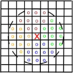
Figure 1: This figure shows the handcrafted neighborhood system used in order to define the context-aware kernels. Red cross stands for a particular cell in the regular grid, and colored circles stand for its 4 different types of neighbors. Here we consider a disk with 4 sectors.

We can show that the optimization problem is Eq. (1) admits the following closed-form kernel solution (details about the proof are omitted in this paper)

$$\mathbf{K}^{(t+1)}=\mathbf{S}+\gamma\sum_{c=1}^{C}\mathbf{P}_{c}\mathbf{K}^{(t)}\mathbf{P}_{c}^{{}^{\prime}},$$ (2)

here $\mathbf{K}^{(0)}=\mathbf{S}$, $\gamma=\alpha/\beta$ with $\alpha/\beta$ chosen in order to guarantee the convergence of the closed-form solution (2) to a fixed-point (which is always observed when $\gamma$ is not very large). Note that when $\mathbf{S}$ is p.s.d, all the resulting closed-form solutions (for different $t$) will also be p.s.d and this results from the closure of the positive semi-definiteness w.r.t. different operations including sum and product. Hence, this kernel solution can be expressed as an inner product $\mathbf{K}^{(t+1)}=\mathbf{\Phi}^{(t+1)^{\prime}}\mathbf{\Phi}^{(t+1)}$ involving maps that take data from their input space to a high dimensional space; one may show that this map $\mathbf{\Phi}^{(t+1)}$ is explicitly and recursively given as

$$\mathbf{\Phi}^{(t+1)}=\Big{(}\mathbf{\Phi}^{{}^{\prime}(0)}\ \ \gamma^{\frac{1}{2}}\mathbf{P}_{1}\mathbf{\Phi}^{{}^{\prime}(t)}\ \ldots\ \ \gamma^{\frac{1}{2}}\mathbf{P}_{C}\mathbf{\Phi}^{{}^{\prime}(t)}\Big{)}^{\prime}.$$ (3)

Here ${\bf\Phi}^{(0)}_{\bf x}={\bf V}_{\bf x}$ (with ${\bf S}_{{\bf x},{\bf x}^{\prime}}={\bf V}^{\prime}_{\bf x}{\bf V}_{\bf x}$) and the subscript in ${\bf{\Phi}}_{{\bf x}}$ denotes the restriction of the map ${\bf{\Phi}}$ to a point ${\bf x}$. According to Eq. (3), it is clear that the mapping ${\bf\Phi}^{(t+1)}$ is not equal to ${\bf\Phi}^{(t)}$ since the dimensionality of the map increases w.r.t. $t$. However, the convergence of the inner product ${\bf\Phi^{\prime}}^{(t+1)}{\bf\Phi}^{(t+1)}$ to a fixed-point is again guaranteed when $\gamma$ is bounded, i.e., the gram matrices of the designed kernel maps are convergent.
Resulting from the definition of the adjacency matrices $\{{\bf P}_{c}\}_{c}$ and from Eq. (3), it is easy to see that building kernel maps could be achieved image per image with obviously the same number of iterations, i.e., the evaluation of kernel maps of a given image is independent from the others and hence not transductive.

Figure 2: This figure shows that the learned kernel maps can be seen as multi-layered maps of increasing dimensionality corresponding to larger and more influencing geometrical context.

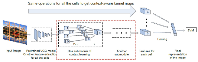
Figure 3: This figure shows the whole architecture and flowchart of our deep context learning. Given an input image (divided into $8\times 10$ cells; as also shown in experiments), cells are first described using the pre-trained VGG CNN. Afterwards, the context-based kernel map of a given cell (for instance cell 0), at a given iteration, is obtained by combining the kernel maps of its neighboring cells (namely cells 1, 2, 3 and 4), obtained at the previous iteration, as shown in the red dashed rectangle and also in Eq. (3). At the end of this iterative process, the kernel maps of all the cells are pooled together in order to obtain the global representation of the input image, prior to achieve its classification. Note that the network shown in the red rectangle, together with the pooling layer, correspond to the DN shown in Fig. 2.

3 Context Learning with Deep Networks

The framework presented in Section 2 is able to design more effective kernels (compared to context-free ones) by taking into account the context. However, this framework is totally unsupervised, so it does not benefit from existing labeled data in order to produce more discriminating kernels; furthermore, the context (and its matrices $\{\mathbf{P}_{c}\}_{c}$) is completely handcrafted. Considering these issues, we propose in this section a method that considers context learning as a part of kernel design using deep networks.

3.1 From context-aware kernels to deep networks

Considering any two samples ${\bf x}$, ${\bf x}^{\prime}$ in $\cal X$ and also the kernel definitions in Eqs. (2) and (3), one may rewrite ${{\bf K}}_{{\bf x},{\bf x}^{\prime}}^{(t)}$ as

$$\begin{array}[]{l}{{\bf K}}_{{\bf x},{\bf x}^{\prime}}^{(t)}=\underbrace{\phi_{t}(\phi_{t-1}(...\phi_{1}(\phi_{0}({\bf x}))))}_{t\ \textrm{times}}.\underbrace{\phi_{t}(\phi_{t-1}(...\phi_{1}(\phi_{0}({\bf x}^{\prime}))))}_{t\ \textrm{times}},\end{array}$$

with $\phi_{t}({\bf x})={\bf\Phi}_{\bf x}^{(t)}$. Following the definition of the convolution kernel ${\cal K}$, at iteration $t$, we have

$$\begin{array}[]{ll}\displaystyle{\cal K}({\cal S}_{p},{\cal S}_{q})&=\displaystyle\sum_{{\bf x}\in{\cal S}_{p}}\sum_{{\bf x}^{\prime}\in{\cal S}_{q}}{{\bf K}}_{{\bf x},{\bf x}^{\prime}}^{(t)}\\ &=\displaystyle\sum_{{\bf x}\in{\cal S}_{p}}\underbrace{\phi_{t}(\phi_{t-1}(...\phi_{1}(\phi_{0}({\bf x}))))}_{t\ \textrm{times}}\\ &\displaystyle\ \ \ \ \ \ \ \ \ \ .\sum_{{\bf x}^{\prime}\in{\cal S}_{q}}\underbrace{\phi_{t}(\phi_{t-1}(...\phi_{1}(\phi_{0}({\bf x}^{\prime}))))}_{t\ \textrm{times}}.\end{array}$$ (4)

Each side of the convolution kernel, in Eq. (4), corresponds to multi-layered feature maps of increasing dimensionality that capture larger and more influencing context, related to points and their geometrical configurations (see Fig. 2). We observe that the architecture in this figure is very similar to the one widely used in deep learning, with some differences residing in the definition of the weights. Indeed, the latter correspond to the values of matrices $\{{\bf P}^{(t)}_{c}\}_{t,c}$ for different iterations and the weights in the final layer correspond to pooling (summation) weights; the latter are equal to $1$ following Eq. (4). In contrast to many usual deep learning algorithms, the weights of this deep network are easy to interpret.

Note that the appropriate number of layers in this network is defined by the asymptotic behavior of our context-aware kernel; indeed, the number of iterations necessary in order to obtain convergence is exactly the number of layers in this deep network. In practice, convergence happens in less than five iterations [36]. Now, considering ${\bf\tilde{K}}$ as the limit of Eq. (2) (for some $t\leadsto T$) and ${\bf\tilde{\Phi}}$ as the underlying kernel map (using Eq. (3)), the new form of the convolution kernel $\cal K$ between two sets of points ${\cal S}_{p}$, ${\cal S}_{q}$ can be rewritten ${\cal K}({\cal S}_{p},{\cal S}_{q})=\sum_{({\bf x},{\bf x}^{\prime})\in{\cal S}_{p}\times{\cal S}_{q}}\langle{\bf\tilde{\Phi}}_{{\bf x}},{\bf\tilde{\Phi}}_{{\bf x}^{\prime}}\rangle$. It is easy to see that $\cal K$ is a p.s.d kernel as it can be rewritten as a dot product involving finite dimensional and explicit maps, i.e., ${\cal K}({\cal S}_{p},{\cal S}_{q})=\langle\phi_{\cal K}({\cal S}_{p}),\phi_{\cal K}({\cal S}_{q})\rangle$, with $\phi_{\cal K}({\cal S}_{p})=\sum_{{\bf x}\in{\cal S}_{p}}{\bf\tilde{\Phi}}_{{\bf x}}$, which clearly shows that each constellation of points ${\cal S}_{p}$ can be deeply represented with the explicit kernel map $\phi_{\cal K}({\cal S}_{p})$ (i.e., the output of the deep network in the Fig. 2).

It is worth noticing that our context learning framework, in spite of being targeted to kernel design, can be achieved ”end-to-end” thanks to the existence of the maps $\phi_{0}(.)$ for many kernels (e.g. linear, histogram intersection, polynomial kernel and other complex kernels); see for instance [23]. Therefore, we adopt back-propagation in order to update the weights of the network in Fig. 2 as described subsequently (see also the flowchart of the whole framework in Fig. 3); interestingly, this framework could also benefit from pre-trained convolutional neural networks (CNN) as input to the kernel map $\phi_{0}(.)$ as also shown through experiments in Section 4.

$r$	Method	BoW features		VGG-CNN features
		Linear kernel	HI kernel	Linear kernel	HI kernel
	Context-free	39.7/24.4/46.6	41.3/25.1/49.5	45.3/30.8/56.4	45.5/30.1/57.9
1	fixed Context-aware ([23])	40.6/24.6/48.3	42.6/26.3/50.5	45.8/31.2/57.6	46.4/30.7/58.5
	learned Context-aware	42.7/26.4/50.5	45.2/26.4/53.9	47.5/32.7/58.7	48.8/32.7/59.9
5	fixed Context-aware ([23])	41.0/25.3/48.9	42.9/26.7/51.3	46.8/31.8/57.9	46.9/31.1/58.7
	learned Context-aware	44.0/26.6/52.0	45.6/26.2/54.0	47.9/33.2/58.8	48.4/32.7/59.5

TABLE I: The performance (in $\%$) of different kernels on ImageCLEF database. A triple $\cdot/\cdot/\cdot$ stands for MFS/MFC/MAP. In these experiments $r$ corresponds to the radius of the disk that supports context.

3.2 Context learning

Considering a multi-class problem with $K$ classes and $N$ training images $\{{\cal I}_{p}\}_{p=1}^{N}$, we define ${\bf Y}_{k}^{p}$ as the membership of the image ${\cal I}_{p}$ to the class $k\in\{1,\dots,K\}$; here ${\bf Y}_{k}^{p}=+1$ iff ${\cal I}_{p}$ belongs to class $k$ and ${\bf Y}_{k}^{p}=-1$ otherwise. We consider in this section, a dynamic and discriminative update of matrices $\{{\bf P}_{c}^{(t)}\}_{c,t}$; first, we plug the explicit form of $\tilde{{\bf\Phi}}$ into $\phi_{\cal K}({\cal S}_{p})$, then we optimize the following objective function (w.r.t. $\{{\bf P}_{c}^{(t)}\}_{c,t}$ with $t=0,\dots,T-1$ and the SVM parameters denoted $\{w_{k}\}_{k}$). This objective function includes the following regularization term and hinge loss

$$\min_{{\bf P}_{c},w_{k}}\displaystyle\sum_{k=1}^{K}\frac{1}{2}||w_{k}||^{2}+C_{k}\sum_{p=1}^{N}\max(0,1-{\bf Y}_{k}^{p}w_{k}^{\prime}\phi_{\cal K}({\cal S}_{p})),$$ (5)

as the optimization of the above objective function w.r.t. the two sets of parameters together is difficult, we adopt an alternating optimization procedure; this is iteratively achieved by fixing one of the two sets of variables and solving w.r.t. the other. When fixing $\{{\bf P}_{c}^{(t)}\}_{c,t}$, the goal is to learn the parameters $\{w_{k}\}_{k}$ of $K$ binary SVM classifiers (denoted $\{f_{k}\}_{k=1}^{K}$). Since kernel map $\phi_{\cal K}({\cal S}_{p})$ of a given image ${\cal I}_{p}$ is explicitly given as the output of the deep network in Fig. 2, each classifier $f_{k}$ can be written as $f_{k}({\cal I})=w_{k}^{\prime}\phi_{\cal K}({\cal S}_{p})$, where $w_{k}$ corresponds to the parameters of the SVM. The optimization of Eq. (5) w.r.t. these parameters $\{w_{k}\}_{k}$ is achieved using LIBSVM [37].

When fixing $\{w_{k}\}_{k}$, the optimization of Eq. (5) is achieved (w.r.t. $\{{\bf P}_{c}^{(t)}\}_{c,t}$) using gradient descent. Let ${E}$ denote the objective function in Eq. (5), the gradient of ${E}$ w.r.t. the final kernel map $\phi_{\cal K}$ (i.e., output of the DN) is

$$\frac{\partial E}{\partial\phi_{\cal K}}=-\sum_{p=1}^{N}\sum_{k=1}^{K}C_{k}{\bf Y}_{k}^{p}w_{k}\mathbbm{1}_{\{1-{\bf Y}_{k}^{p}w_{k}^{\prime}\phi_{\cal K}({\cal S}_{p})\}},$$ (6)

here $\mathbbm{1}_{\{\}}$ is the indicator function. From Eq. (3), it can be seen that the gradient of ${E}$ w.r.t. $\{{\bf P}_{c}^{(T-1)}\}_{c,T-1}$ can be computed as the sum of gradients over all the cells in the regular grid. This gradient is backward propagated to the previous layers using the chain rule [38] in order to (i) obtain gradients w.r.t. adjacency matrices $\{{\bf P}_{c}^{(t)}\}_{c,t}$, for $t=T-1,\dots,0$ (weights of the deep network in Fig. 2), and (ii) update these weights using gradient descent.
Finally, the two steps of this iterative process are repeated till convergence is reached, i.e., when the values of these two sets of parameters remain unchanged. In practice, this convergence is observed in less than 100 iterations.

4 Experimental Validation

We evaluate the performance of our context and kernel learning method on the challenging ImageCLEF benchmark [11]. The targeted task is image annotation; given an image, the goal is to predict the list of concepts present into that image. These concepts are declared as present iff the underlying SVM scores are positive.

The dataset of this benchmark is large and includes more than 250k images; we only use the dev set (which includes 1,000 images) as the ground truth is released for this subset only. Images of this subset belong to 95 categories (concepts); as these concepts are not exclusive, each image may be annotated with one or multiple concepts. We randomly split the dev set into two subsets (for training and testing). We process each image in the training and testing folds by re-scaling its dimensions to $400\times 500$ pixels and partitioning its spatial extent into $8\times 10$ cells; each cell includes $50\times 50$ pixels. Two different representations are adopted in order to describe each cell: i) Bag-of-Words (BoW) histogram (of 500 dimensions) over SIFT features, where the codewords of this histogram are pre-trained offline using K-means; and ii) Deep features based on the pre-trained VGG model on the ImageNet database (“imagenet-vgg-m-1024”) [39]. Our purpose here is to investigate the adaptability of the proposed framework both with handcrafted and pre-trained CNN features.

Kernel	MF-S	MF-C	mAP
GMKL([40])	41.3	24.3	49.1
2LMKL([41])	45.0	25.8	54.0
LDMKL ([42])	47.8	30.0	58.6
The proposed context-aware	48.8	32.7	59.9

TABLE II: This table shows comparison of performances (in %) between different kernel-learning methods.

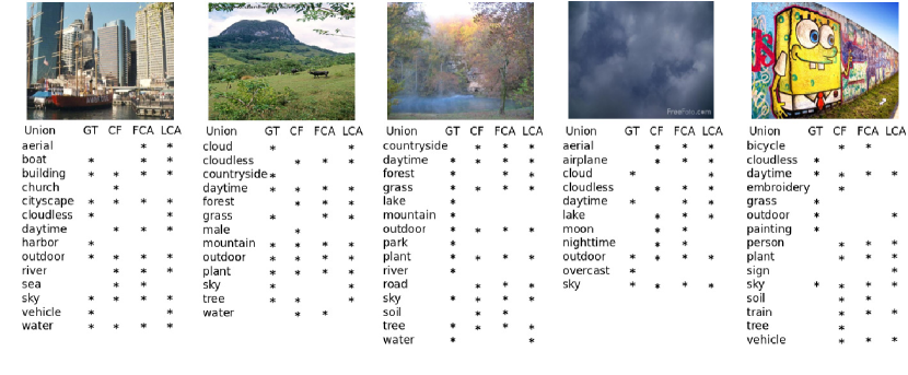
Figure 4: Examples of annotation results using context-free kernels (“CF”), context-aware kernels with fixed and learned context (resp. “FCA” and ”LCA”). “GT” refers to ground truth annotation while the stars stand for the presence of a given concept in the test image.

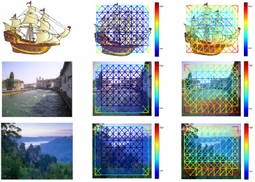
Figure 5: This figure shows original images (left), handcrafted (middle) and learned contexts (right) between $8\times 10$ cells (with $r=1$). For each cell, the importance of its context is shown with colored connections to its neighboring cells; warm colors stand for important relationships while cold colors stand for less important ones. In the handcrafted context, adjacency matrices $\{\mathbf{P}_{c}\}_{c}$, are set to be row-stochastic, and this is obtained by normalizing each row (cell) in these matrices by the number of its spatial neighbors that’s why cells in the four corners have larger values (better viewed/zoomed in PDF)

We consider four types of geometric relationships in order to build our context-aware kernel maps (see again Fig. 1). As the dimensionality of the DN (in Fig. 2) increases rapidly with the layers, we adopt in our experiments an architecture depth that provides a reasonable balance between dimensionality and performance as well as convergence of kernel map evaluation; hence, we chose an architecture with 3+1 layers where the last one corresponds to pooling (again following Fig. 2). In these experiments, we consider linear and histogram intersection maps as – context-free kernel map – initialization of our DN; note that the explicit maps of linear and histogram intersection kernels correspond to identity and decimal-to-unary mapping respectively (see [36] for more details about these maps).

Using the setting above, we learn multi-class SVMs for different concepts (using the training fold) on top of the learned context-aware kernel maps, and we evaluate their performances on the testing fold. These performances are measured using the F-scores (harmonic means of recall and precision) at the sample and concept levels (denoted MFS and MFC respectively) as well as the mean average precision (MAP); higher values of these measures imply better performances. Tab. I shows a comparison of our context-aware kernels against context-free ones, with handcrafted and learned contexts on top of the BoW features as well as the deep VGG features. From these results the gain obtained with the learned context is clear both w.r.t. handcrafted context and when no context is used. Tab. II shows performance comparison of our learned context-aware kernel against other kernel learning methods on the ImageCLEF database; from these results a clear gain is obtained when learning context. Fig. 4 shows a sample of images and their annotation results using context-free and context-aware kernels with fixed (handcrafted) and learned context. Finally, Fig. 5 is a visualization of handcrafted and learned contexts superimposed on three images from ImageCLEF; when context is learned, it is clear that some spatial cell context relationships are amplified while others are attenuated and this reflects their importance in kernel learning and image classification.

5 Conclusion

We introduced in this paper a novel method that considers context learning as a part of kernel design. The method is based on a particular deep network architecture which corresponds to the map of our context-aware kernel solution. In this contribution, relevant context is selected by learning weights of a DN; indeed high weights correspond to the relevant parts of the context while small weights are related to the irrelevant parts. Experiments conducted on the challenging ImageCLEF benchmark, show a clear gain of SVMs trained on top of kernel maps (with learned context) w.r.t. SVMs trained on top of kernel maps (with handcrafted context) and context-free kernels.

References

- [1] K. Barnard, P. Duygulu, N. de Freitas, and D. Forsyth, “Matching words and pictures,” JMLR, vol. 3, 2003.
- [2] A. Makadia, V. Pavlovic, and S. Kumar, “A new baseline for image annotation,” in ECCV, 2008, pp. 316–329.
- [3] N. Boujemaa, F. Fleuret, V. Gouet, and H. Sahbi, “Visual content extraction for automatic semantic annotation of video news,” in the proceedings of the SPIE Conference, San Jose, CA, vol. 6, 2004.
- [4] P. Vo and H. Sahbi, “Transductive kernel map learning and its application to image annotation,” in BMVC, 2012, pp. 1–12.
- [5] H. Sahbi, “Cnrs-telecom paristech at imageclef 2013 scalable concept image annotation task: Winning annotations with context dependent svms.” in CLEF (Working Notes), 2013.
- [6] K. Goh, E. Chang, and B. Li, “Using one-class and two-class svms for multiclass image annotation,” IEEE transcation on Knowledge and Data Engineering, vol. 17, 2005.
- [7] X. Qi and Y. Han, “Incorporating multiple svms for automatic image annotation,” IEEE Transcations on Knowledge and Data Engineering, vol. 40, 2007.
- [8] H. Sahbi and N. Boujemaa, “Coarse-to-fine support vector classifiers for face detection,” in Pattern Recognition, 2002. Proceedings. 16th International Conference on, vol. 3. IEEE, 2002, pp. 359–362.
- [9] M. Guillaumin, T. Mensink, J. Verbeek, and C. Schmid, “Tagprop: Discriminative metric learning in nearest neighbor models for image auto-annotation,” in ICCV, 2009, pp. 316–329.
- [10] Y. Verma and C. Jawahar, “Image annotation using metric learning in semantic neighbourhoods,” in ECCV, 2012.
- [11] M. Villegas, R. Paredes, and T. B., “Overview of the imageclef 2013 scalable concept image annotation subtask,” CLEF Conference, 2013.
- [12] J. Shawe-Taylor and N. Cristianini, “Kernel methods for pattern analysis,” Cambriage University Press, 2004.
- [13] F. Bach, G. Lanckriet, and M. Jordan, “Multiple kernel learning, conic duality, and the smo algorithm,” in ICML, 2004.
- [14] M. Jiu and H. Sahbi, “Semi supervised deep kernel design for image annotation,” in ICASSP, 2015.
- [15] ——, “Laplacian deep kernel learning for image annotation,” in ICASSP, 2016.
- [16] A. Vedaldi and A. Zisserman, “Efficient additive kernels via explicit feature maps,” IEEE Transactions on PAMI, vol. 34, 2012.
- [17] S. Thiemert, H. Sahbi, and M. Steinebach, “Applying interest operators in semi-fragile video watermarking,” in Security, Steganography, and Watermarking of Multimedia Contents VII, vol. 5681. International Society for Optics and Photonics, 2005, pp. 353–363.
- [18] S. Belongie, J. Malik, and J. Puzicha, “Shape matching and object recognition using shape contexts,” IEEE Transactions on PAMI, vol. 24, pp. 509–522, 2001.
- [19] X. He, R. Zimel, and M. Carreira, “Multiscale conditional random fields for image labeling,” in CVPR, 2004.
- [20] H. Sahbi, J.-Y. Audibert, and R. Keriven, “Context-dependent kernels for object classification,” PAMI, vol. 33, pp. 699–708, 2011.
- [21] M. Jiu, C. Wolf, G. Taylor, and A. Baskurt, “Human body part estimation from depth images via spatially-constrained deep learning,” Pattern Recognition Letteres, vol. 50, pp. 122–129, 2014.
- [22] X. Li and H. Sahbi, “Superpixel-based object class segmentation using conditional random fields,” in Acoustics, Speech and Signal Processing (ICASSP), 2011 IEEE International Conference on. IEEE, 2011, pp. 1101–1104.
- [23] H. Sahbi, “Explicit context-aware kernel map learning for image annotation,” in ICVS, 2013.
- [24] ——, “Imageclef annotation with explicit context-aware kernel maps,” in International Journal of Multimedia Information Retrieval, 2014.
- [25] H. Sahbi and X. Li, “Context-based support vector machines for interconnected image annotation,” in Asian Conference on Computer Vision. Springer, 2010, pp. 214–227.
- [26] F. Yuan, G.-S. Xia, H. Sahbi, and V. Prinet, “Mid-level features and spatio-temporal context for activity recognition,” Pattern Recognition, vol. 45, no. 12, pp. 4182–4191, 2012.
- [27] G. Hinton, S. Osindero, and Y.-W. Teh, “A fast learning algorithm for deep belief nets,” Neural Computation, 2006.
- [28] Y. Bengio and P. Lamblin, “Greedy layer-wise training of deep networks,” in NIPS, 2007.
- [29] Y. Bengio, “Learning deep architectures for AI,” Foundations and Trends in Machine Learning, vol. 2, no. 1, 2009.
- [30] A. Krizhevsky, I. Sutskever, and G. E. Hinton, “Imagenet classification with deep convolutional neural networks,” in NIPS, 2012.
- [31] Y. Zhang, M. Bai, P. Kohli, S. Izadi, and J. Xiao, “Deepcontext: Context-encoding neural pathways for 3d holistic scene understanding,” in ICCV, 2017.
- [32] W.-C. Hung, Y.-H. Tsai, X. Shen, Z. Lin, K. Sunkavalli, X. Lu, and M.-H. Yang, “Scene parsing with global context embedding,” in ICCV, 2017.
- [33] D. Li, X. Chen, Z. Zhang, and K. Huang, “Learning deep context-aware features over body and latent parts for person re-identification,” in CVPR, 2017.
- [34] J. Mairal, P. Koniusz, Z. Harchaoui, and C. Schmid, “Convolutional kernel networks,” in NIPS, 2014.
- [35] M. Jiu and H. Sahbi, “Deep kernel map networks for image annotation,” in ICASSP, 2016.
- [36] H. Sahbi, “Imageclef annotation with explicit context-aware kernel maps,” International Journal of Multimedia Information Retrieval, 2015.
- [37] C.-C. Chang and C.-J. Lin, “Libsvm: A library for support vector machines,” ACM Transactions on Intelligent Systems and Technology, vol. 2, pp. 1–27, 2011.
- [38] Y. LeCun, L. Botto, Y. Bengio, and P. Haffner, “Gradient-based learning applied to document recognition,” Proceedings of IEEE, vol. 86, no. 11, pp. 2278–2324, 1998.
- [39] K. Chatfield, K. Simonyan, A. Vedaldi, and A. Zisserman, “Return of the devil in the details: Delving deep into convolutional nets,” in BMVC, 2014.
- [40] M. Varma and B. Babu, “More generality in efficient multiple kernel learning,” ICML, 2009.
- [41] J. Zhuang, I. Tsang, and S. Hoi, “Two-layer multiple kernel learning,” in ICML, 2011, pp. 909–917.
- [42] M. Jiu and H. Sahbi, “Nonlinear deep kernel learning for image annotation,” IEEE Transactions on Image Processing, vol. 26(4), 2017.