Nonlinear Deconvolution by Sampling Biophysically Plausible Hemodynamic Models

Abstract

Non-invasive methods to measure brain activity are important to understand cognitive processes in the human brain. A prominent example is functional magnetic resonance imaging (fMRI), which is a noisy measurement of a delayed signal that depends non-linearly on the neuronal activity through the neurovascular coupling. These characteristics make the inference of neuronal activity from fMRI a difficult but important step in fMRI studies that require information at the neuronal level. In this article, we address this inference problem using a Bayesian approach where we model the latent neural activity as a stochastic process and assume that the observed BOLD signal results from a realistic physiological (Balloon) model. We apply a recently developed smoothing method called APIS to efficiently sample the posterior given single event fMRI time series. To infer neuronal signals with high likelihood for multiple time series efficiently, a modification of the original algorithm is introduced. We demonstrate that our adaptive procedure is able to compensate the lacking of inputs in the model to infer the neuronal activity and that it outperforms dramatically the standard bootstrap particle filter-smoother in this setting. This makes the proposed procedure specially attractive to deconvolve resting state fMRI data. To validate the method, we evaluate the quality of the signals inferred using the timing information contained in them. APIS obtains reliable event timing estimates based on fMRI data gathered during a reaction time experiment with short stimuli. Hence, we show for the first time that one can obtain accurate absolute timing of neuronal activity by reconstructing the latent neural signal.

1 Introduction

Functional magnetic resonance imaging (fMRI) is an important method to investigate sensory, motor and cognitive functions of the human brain. This non-invasive technique to measure brain activity provides indirect signals of the underlying neuronal dynamics because it measures hemodynamic responses that represent changes in blood flow and oxygenation levels.

Inverting the non-linear hemodynamic system is important to understand aspects of cognitive functions and for connectivity analysis at the neuronal level. Nevertheless, reconstructing the brain activity from the fMRI signal presents many challenges. For instance, the measured signals might have components from non-neuronal hemodynamic sources that can affect causal connectivity estimates [5]. Moreover, the general inverse problem, also known as blind deconvolution, is ill-posed because both the true parameters of the hemodynamic system and the latent inputs are unknown. Therefore, given the fMRI time course, the reconstruction of the neuronal signal is not unique. The reason for this is that the hemodynamic parameters determine the delay of the BOLD signal with respect to the underlying neuronal activity giving a continuum of possible solutions.

Activation studies employing general linear models (GLM) circumvent this problem by using multiple repetitions of the same stimulus and a canonical hemodynamic response function (HRF) together with time and dispersion derivatives or basis functions that correct the HRF [12, 13]. In these cases, temporal information and the exact shape of the HRF are less likely to be crucial, the models may not be very sensitive to temporal nuances in the data and are usually not used to estimate the latent neuronal dynamics.

A very different approach to model the hemodynamic transformation is to use physiologically informed models of BOLD responses, such as the Balloon model [3, 14]. Although this is a complex, highly parametrized biophysical model, it is useful for jointly estimating the latent neuronal process and the hemodynamic transformation, for instance with the well-known dynamic causal modeling (DCM) [15] which assumes a latent state space model (SSM). This deterministic method can be generalized to a probabilistic method, i.e. stochastic DCM [27, 4].

The biological inspired models posses a rich HRF variability that linear models do not capture. For instance, there is evidence of nonlinear effects in the BOLD signal for high frequency stimulus presentations [1, 41] and different stimuli durations, e.g. when linear models are used, responses to $200\ ms$ stimuli are underestimated [6]. Therefore, non-linearities in the hemodynamic system are important whenever we wish to estimate the hidden neuronal activity and sophisticated fMRI analysis requires methods that can handle these effects properly.

Estimating parameters of the biological plausible models involves usually a maximum likelihood approach that requires the computation of gradients with respect to the parameters. If these parameters affect the noisy degrees of freedom, the computation of their gradient is straight forward in the well-known Expectation-Maximization algorithm (EM) for time series [35]. For deterministic degrees of freedom, one needs to resort to one of the following methods to compute the gradient [37]. The simplest approach, currently used in DCM, is the finite difference method. An alternative uses implicit differentiation of the error function with respect to the relevant parameters. This gives a set of differential equations that are integrated together with the forward model to compute the gradient. This method–called Forward Sensitivity (FS) method–was proposed in [6] in the context of fMRI data. However, neither the reliability of this method for fMRI data nor the resulting differential equations were discussed in detail.

The computation of the gradients to maximize the likelihood involves the estimation of the hidden variables. This latent state estimation is a problematic step where most of the methods differ. Until now, there are roughly speaking three families of approaches for estimating the latent process in the context of fMRI data.

First, particle methods sample the dynamics in a forward and (possibly) a backward pass to obtain Monte Carlo estimates of the posterior density. As the number of samples (particles) grows, the estimates become more accurate, however the computational cost of the backward pass makes these methods unpractical in many cases [2, 7, 30]. Moreover, it has been shown that the method proposed here outperforms the vanilla implementations of particle filter methods, namely the bootstrap filter-smoother and the forward-backward smoother Ruiz and Kappen [36]. In [32, 21], methods of this family were applied to estimate hidden neuronal and hemodynamic states from fMRI data.

Second, variational Bayesian methods approximate the posterior distribution with a variational density that maximizes a lower bound on the evidence. This has been applied in the context of fMRI data in the dynamic expectation maximization algorithm and its generalizations, which use models formulated in terms of generalized coordinates of motion [11, 10, 16].

Third, Gaussian methods approximate the posterior distributions by Gaussians under the assumption that one can obtain a consistent minimum variance estimator by recursive propagation and update of the mean and variance of the target densities. Important examples are the extended Kalman filter and the unscented Kalman filter. For fMRI data, [34] used the local linearization filter [20]. More recently, [18] proposed an estimation scheme using cubature Kalman filtering in the forward pass and a cubature Rauch-Tung-Striebel smoother in the backward pass.

Interestingly, the methods mentioned above [16, 18, 34] are the only available techniques applied to fMRI data shown capable of estimating the inputs together with the hidden states. This is important because the assumption of known exogenous inputs does not always hold–for instance in resting state fMRI data there are no stimuli present during the measurements–or it might be an implausible assumption for higher cognitive areas [29]. However, it is not clear how accurate these methods are for different stimulus durations and frequency, because either they need restrictive parameterization of the inputs [34], or the experimental design on which they were tested had stimulus durations of several seconds and hence, their validity is restricted to inputs of the same time scale as the BOLD signal [39, 16].

A precise measure of the timing of brain activity is important to better understand the neural substrate of cognitive processes in the brain. Detecting correct input timings to the brain regions from fMRI measurements may help in our understanding of mental chronometry, i.e. the sequential patterns of brain activity involved during cognitive processes. A prominent example for the need of precise sequential information is the reconstruction of causal interactions among brain regions [15]. Although it has been shown that small relative timings differences are detectable in a given location [31, 28, 9, 26], it is generally thought that accurate measurements of the absolute timing of neuronal activity is not feasible. Indeed, due to the indirect measurement procedure involved in fMRI and the ill-defined nature of the blind deconvolution problem, this is an extremely challenging problem.

To the best of our knowledge, there is no analysis available on the precision of absolute input timing estimates from real fMRI data, especially for very short stimuli in the order of hundreds of milliseconds. Interesting work in this direction is found in [18]. There, examples of estimations on synthetic data using short inputs were obtained but there was no analysis on the precision of the input timings recovered. Due to the lack of a ground truth that guides the validation of methods when applied to real fMRI time series, we believe that the timing estimates of short stimuli is an important aspect when considering validating methods of fMRI deconvolution. Furthermore, analyzing the errors in absolute timings is also an important tool to asses the quality of the estimates for the hemodynamic parameters that influence the delay in the response.

Outline

In this article, we estimate the neuronal activity and absolute input timings in individual regions of interest (ROIs) from single-event fMRI time series gathered in a reaction time experiment with very short stimuli ($150\ ms$). First, we analyze in detail the sensitivity of the BOLD delay to changes in the hemodynamic parameters to identify the most relevant parameters affecting the delay of the BOLD signal relative to the input. We then derive the differential equations involved in the estimation of these parameters via the FS method. Here, we assume deterministic dynamics and that the input is known. In addition, we analyze and evaluate this method using synthetic data and estimate the relevant parameters for the fMRI time series to improve the timing estimates of unknown inputs.

Second, we show the feasibility of latent state estimation for fMRI time series using APIS with excellent sampling efficiency. This is non-trivial because of the complex (Balloon) observation model. In [36] we showed that the APIS method significantly outperforms particle filtering/smoothing methods on complex time series inference tasks. We thus demonstrate that the advantage of APIS over particle filtering methods, in terms of efficiency and accuracy, also applies to fMRI time series data. In addition, during the input estimation procedure we adapt the neuronal noise variance using EM. This is an important and novel step to maximize the data likelihood for a large amount of time series at once and to obtain estimates of the neuronal activity with large amplitudes and accurate event timings.

To validate our method, we compare the estimated timing errors with errors obtained when synthetic data is used, i.e. when the ground truth model is known. We show that, given sufficiently accurate estimates of the hemodynamic parameters, the proposed method can infer the absolute input timing of single events reliably by reconstructing the hidden neuronal activity.

2 Method

2.1 fMRI Data

We analyze fMRI time series obtained from the experimental setting in [33], consisting of subjects reacting to the occurrence of either a visual stimulus (V), an auditory stimulus (A) or a simultaneous combination of both stimuli (AV). Whenever the subjects perceived the stimulus, they had to press a button as fast as possible. The modality of the stimulus presented was random and had a duration of $150\ ms$. We denote the presentation of a stimulus or the reaction as an "event" in the sensory or motor ROIs respectively.

We consider only the first subject of this study, who participated in two trials. Each trial consisted of 30 stimuli presented at a rate of 1 stimulus per $16\ s$ (with some jitter of 0.2 seconds). The response times were recorded and the temporal resolution of the acquisition was $TR=0.4\ s$. Because this work focuses on single trial measurements, the data is denoised using manual independent component classification as proposed in [17]. A standard GLM analysis is then used to delineate the motor, auditory and visual cortex used in this task. Regions of interest of about 500 voxels ($2mm$ isotropic) are defined for the audio (A ROI), visual (V ROI) and left motor cortices (M ROI) and time series extracted from them. The time series of subjects 2 and 3 are too noisy when performing a standard GLM analysis and have to be discarded.

We estimate the neuronal activity around each event separately. For this, the original time course is divided in 30 segments of length $T=16\ s$ around the event time. This amounts to 41 observations in each time series (the first defining $t=0$) and the event time falls around $3.2$ seconds.

To characterize the relative BOLD change $\left\{\hat{y}_{i}\right\}_{i=1,\dots,41}$, each time course $\left\{y_{i}\right\}_{i=1,\dots,41}$ is centralized and normalized by the mean $\mu_{y}$ of its "null" distribution,

$$\hat{y}_{i}=\frac{y_{i}-\mu_{y}}{\mu_{y}}.$$

The "null" distribution of each time series is defined as the set of data points outside a time window after the stimulus, when the neuronal activity is assumed to have the baseline value ($z_{t}=0$). The window is chosen such that the variance of the data points included is minimal and is estimated for each event separately to account for long time scale fluctuations in the data.

2.2 Modeling the BOLD Signal

Similar to [14], we consider a single region with a 5-dimensional dynamic state $x=(z,s,f,q,v)$. However, unless stated otherwise, the neuronal activity $z$ follows stochastic dynamics given by

$$dz=-A(z-u(z_{t},t))dt+\sqrt{A}\sigma_{z}dW_{z}$$ (1)

The parameter $A$ sets the time scale of the neuronal response and $dW_{z}\sim N(0,dt)$ is a Wiener process with variance $dt=0.01$. According to the literature, typical values observed for the neuronal lags are around $5-35\ ms$ [38]. We set $A$ such that the system has a characteristic time scale of $1/A=20\ ms$, but our results are robust against changes in $A$. The term $\sqrt{A}$ in the noise ensures that the stationary distribution remains invariant to the time scale.

Notice that we define process (1) to have an unknown input $u(z,t)$ that we wish to estimate. In general, $u(z,t)$ can be any parametrized function [25], but in this paper it was chosen to have the simple form $u(z,t)=I_{z}(t)z+I_{t}(t)$ with $I_{z}(t)$ and $I_{t}(t)$ as time varying functions to be learned [36].

The neuronal activation $z_{t}$ is passed through the following nonlinear deterministic transformation defining the dynamics of the other four variables; two Hemodynamic equations [14]

$$ds =\left(\epsilon z-\frac{s}{\tau_{s}}-\frac{f-1}{\tau_{f}}\right)dt$$ (2)

$$df =sdt$$

and two equations of the Balloon model [3],

$$dq =\frac{1}{\tau_{0}}\left(f\frac{1-(1-E_{0})^{1/f}}{E_{0}}-v^{(1/\alpha)-1}q\right)dt$$ (3)

$$dv =\frac{1}{\tau_{0}}\left(f-v^{1/\alpha}\right)dt.$$

The BOLD signal change is given by

$$\hat{y}(t)=B(q_{t},v_{t}|\vartheta)+\sigma_{y}dW_{y}$$ (4)

where $B(q_{t},v_{t}|\vartheta):=V_{0}\left[k_{1}\left(1-q_{t}\right)+k_{2}\left(1-\frac{q}{v}\right)+k_{3}\left(1-v\right)\right]$ and $\vartheta$ denotes all parameters of the system.

In addition, we consider as prior for the initial condition $x_{0}=(z_{0},s_{0},f_{0},q_{0},v_{0})$ a normal distribution with mean $\mu_{0}=(\mu_{z,0},\mu_{s,0},\mu_{f,0},\mu_{q,0},\mu_{v,0})$ and a covariance given by a diagonal matrix with small entries $\sigma_{z,s,f,q,v,0}^{2}$.

In this article, the parameters of the model were fixed based on [19], with the exception of $\tau_{0}$, $\tau_{f}$ and the neuronal lag $1/A$. These are given in table 1, where the values marked with TBD are to be determined. The values for $k_{1,2,3}$ correspond to those for a gradient echo (GE) sequence at a field strength of $7\ T$ with an echo time of $TE=26\ ms$, according to the settings in [33].

Parameter	Value	Parameter	Value	Parameter	Value	Parameter	Value
$A$	50 Hz	$\sigma_{z}$	TBD	$\mu_{z,0}$	$0$	$\sigma_{z,0}$	$\sigma_{z}/\sqrt{2}$
$\epsilon$	0.8	$E_{0}$	0.4	$\alpha$	0.32	$\sigma_{s,0}$	TBD
$\tau_{s}$	1.54	$k_{1}$	8.4	$V_{0}$	0.04	$\sigma_{f,q,v,0}$	TBD
$\tau_{f}$	TBD	$k_{2}$	0	$\mu_{s,0}$	$0$	$\sigma_{y}$	TBD
$\tau_{0}$	TBD	$k_{3}$	1	$\mu_{f,q,v,0}$	$1$

Table 1: Parameters for the neural dynamics (top row) and for the BOLD transformation (bottom rows).

2.3 Estimating the Parameters of the Model

We estimate the observation noise for each time series from its null distribution. This gives for each case a slightly different noise estimate around $\sigma_{y}\simeq 0.002$.

The variance of the initial state $x_{0}$ is set to the variance of the stationary distribution induced by the Ornstein-Uhlenbeck process for the uncontrolled dynamics in eq. (1) when $u(z,t)=0$. Hence, the variance for $p(z_{0})$ is $\sigma_{z,0}=\sigma_{z}/\sqrt{2}$ and all others are estimated by forward sampling of the system. Because all other dynamic variables are deterministic, the stationary distribution defining our prior over the process is determined by a single free parameter $\sigma_{z}$, the noise of the neuronal activity. This free parameter is adapted to infer inputs that maximize the likelihood.

2.3.1 Forward Sensitivity Equations

The hemodynamic parameters are estimated using the Forward Sensitivity method. The negative log-likelihood or "total cost" $C(\vartheta)=\int_{0}^{T}c_{t}(\vartheta)dt$ is an implicit function of the parameters $\vartheta$ in our model, where $c_{t}(\vartheta)=\sum_{t_{obs}}\delta(t-t_{obs})[\hat{y}_{t}-B(q_{t},v_{t}|\vartheta)]^{2}/2\sigma_{y}^{2}$ summing over the observation times $t_{obs}=t_{1},\dots,t_{41}$. Thus, given an infinitesimal change $\delta\vartheta$ we can expressed the change in $c_{t}(\vartheta)$ at each time point $t\in[0,T]$ by

$$\delta c_{t}=\frac{\partial c_{t}}{\partial q_{t}}\delta q_{t}+\frac{\partial c_{t}}{\partial v_{t}}\delta v_{t}+\sum_{i}\frac{\partial c_{t}}{\partial\vartheta_{i}}\delta\vartheta_{i}$$

where $\delta q_{t},\delta v_{t}$ also depend on $\vartheta$ and are obtained by the variation of the hemodynamic states $q_{t},v_{t}$ w.r.t. $\vartheta$.

We only consider changes in $\tau_{f}$ and $\tau_{0}$ since these parameters have a strong effect on the delay between peaks of the neuronal activity and the BOLD signal, keeping all other parameters fixed. However, the following analysis can be done for any other parameters in the hemodynamic model.

The aim is to obtain the derivatives of $C(\tau_{f},\tau_{0})$ by integrating a system of differential equations for "bar" variables $\bar{q}_{0}(t)=dq_{t}/d\tau_{0},\ \bar{v}_{0}(t)=dv_{t}/d\tau_{0}$ and $\bar{q}_{f}(t)=dq_{t}/d\tau_{f},\ \bar{v}_{f}(t)=dv_{t}/d\tau_{f}$. The total cost is used to update the parameters $\tau_{f,0}$ in a gradient descent fashion. From the variation $\delta\tau_{0}$ we obtain the total derivative of $dc_{t}/d\tau_{0}$,

$$\frac{dc_{t}}{d\tau_{0}}=\frac{\partial c_{t}}{\partial q_{t}}\bar{q}_{0}(t)+\frac{\partial c_{t}}{\partial v_{t}}\bar{v}_{0}(t)$$

where $\bar{q}_{0}(t),\bar{v}_{0}(t)$ follow the dynamic equations,

$$\dot{\bar{q}}_{0}=-\frac{1}{\tau_{0}}\left(\dot{q}+v^{1/\alpha-1}\bar{q}_{0}+(\frac{1}{\alpha}-1)v^{1/\alpha-2}q\bar{v}_{0}\right)$$

$$\dot{\bar{v}}_{0}=-\frac{1}{\tau_{0}}\left(\dot{v}+\frac{1}{\alpha}v^{1/\alpha-1}\bar{v}_{0}\right)$$

The total derivative $dc_{t}/d\tau_{f}$ obtained by the variation $\delta\tau_{f}$ is

$$\frac{dc_{t}}{d\tau_{f}}=\frac{\partial c_{t}}{\partial q_{t}}\bar{q}_{f}(t)+\frac{\partial c_{t}}{\partial v_{t}}\bar{v}_{f}(t)$$

where $\bar{q}_{f}(t),\bar{v}_{f}(t)$ follow

$$\dot{\bar{s}}_{f}=-\frac{1}{\tau_{s}}\bar{s}_{f}-\frac{1}{\tau_{f}}\left(\bar{f}_{f}+\frac{f-1}{\tau_{f}}\right)$$

$$\dot{\bar{f}}_{f}=\bar{s}_{f}$$

$$\dot{\bar{v}}_{f}=-\frac{1}{\tau_{0}}\left(\frac{1}{\alpha}v^{1/\alpha-1}\bar{v}_{f}-\bar{f}_{f}\right)$$

$$\dot{\bar{q}}_{f}=-\frac{1}{\tau_{0}}\left(v^{1/\alpha-1}\bar{q}_{f}+(\frac{1}{\alpha}-1)v^{1/\alpha-2}q\bar{v}_{f}-\bar{E}(f)\bar{f}_{f}\right)$$

with $\bar{E}(f):=E(f)+\ln(1-E_{0})\frac{(1-E_{0})^{1/f}}{E_{0}f}$.

Having the above extended system of differential equations, we can initialize the bar variables to zero and integrate the entire system forward in time. After integration on the interval $t\in[0,T]$, we update the parameters using $dC/d\tau_{0}$ and $dC/d\tau_{f}$ respectively. This is done iteratively until convergence of the parameters.

Before applying this estimation procedure to real data, we validate it on synthetic data generated by numerical integration of a deterministic system ($\sigma_{z}=0$). As input to the system we use a box function with $150\ ms$ length and an on-set time at 3.2 seconds. The amplitude of the input is set to 1. The ground truth values of the parameters are taken to be those in table 1 together with $\tau_{0}=1.02$, $\tau_{f}=2.44$. To generate the synthetic data from this model, a realistic scenario is considered with $TR=0.4$ and a Gaussian measurement noise of $\sigma_{y}=0.002$. For the estimation procedure, the parameters $\tau_{0}^{(0)},\tau_{f}^{(0)}$ are initialized randomly from a log-normal distribution s.t. its log-transformed distribution has variance $0.6$ and mean $(\log\tau_{0}^{(0)},\log\tau_{f}^{(0)})=(0.4,0)$. All other parameters of the system are fixed to the ground truth values.

After validation of the FS method on synthetic data, we fit the parameters $\tau_{0},\tau_{f}$ to the mean fMRI time series of each ROI (A,V,M) in trial 1 and assuming an input to that ROI. The resulting models are used to estimate the input timing of individual time series in trial 2 without any assumptions on the inputs.

Since the sensory ROI A and V do not respond or respond very weakly to the stimulus modality V and A respectively, we do not consider these events when estimating the parameters of the corresponding ROI. Hence, for the auditory and visual regions, there are only 20 signals available in each ROI. On the contrary, all stimuli elicit responses in the motor ROI so we use all 30 events to compute the mean BOLD response. The input to the model for all ROIs is also a box function. For the A and V regions, the on-set time is the mean event time of all the relevant time series. The on-set time of the input to the motor ROI is considered to be the mid-time between the mean stimulus and reaction times.

2.4 Hidden State Estimation

Given an fMRI time series $\hat{y}_{0:T}=\{\hat{y}_{0},\hat{y}_{t_{1}},\dots,\hat{y}_{T}\}$ we are interested in an efficient estimation of the posterior $p(z_{[0,T]}|\hat{y}_{0:T})$, where the prior $p(z_{[0,T]})$ is given by (1) and $z_{[0,T]}$ denotes the continuous path or process from time $t=0$ to $t=T$. The likelihood is given by the observation model (2)-(4).

The posterior or smoothing distribution can be seen as the solution to a stochastic optimal control problem [8, 24]. Using this relation we express the problem of estimating the posterior over the neuronal activity as a Path Integral control problem [22, 23].

Recent results in [36] show that having a sufficiently good parametrization of the control improves dramatically the efficiency of sampling in terms of the effective sample size. This efficiency is achieved with an adaptive importance sampling method called APIS. The sampler learns iteratively a time dependent feedback controller to adapt the process such that the likelihood of the samples increase. This in turn reduces the variance of the importance weights and increases the effective sample size.

Roughly, APIS works as follows. At each iteration, $N$ samples are initialized with a Gaussian prior $p(x_{0})$. The samples are propagated in time by integrating the (stochastic) dynamic equations (1)-(3). The sampled paths $\left\{z_{[0,T]}^{i}\right\}_{i=1,\dots,N}$ are used to compute statistics over the posterior using the respective importance weights obtained from the likelihood and a quadratic control cost acting as a regularizer of the control function $u(z,t)$. Using these statistics, the values $I_{z}(t),I_{t}(t)$ are updated at each time point to estimate the control/input function used in the next iteration. This is repeated until convergence of the effective sample size.

In summary, we use importance sampling adaptively to estimate the hidden diffusion process by regarding the input $u(z,t)=I_{z}(t)z+I_{t}(t)$ as a control function to be estimated. A good approximation of $u(z,t)$ allows steering the samples such that the resulting BOLD signal has high likelihood. We refer the interested reader to [36] for further details.

2.5 Noise Adaptation

One of the features of path integral control theory is that the difference between the posterior distribution relative to the prior process strongly depends on the noise level $\sigma_{z}$. The control is proportional to $\sigma_{z}$. Thus, if $\sigma_{z}$ is small, the control will be small and the posterior deviates only slightly from the prior. This affects directly the likelihood under a strong model mismatch. For instance, if we do not model any input to the neuronal system, the prior is the stationary distribution. Ideally, the controller must adapt the system such that first, the efficiency of the sampler increases and, second, the model mismatch is overcome. This requires strong controllers capable of acting as input signals. However, it is not clear a priori the amount of noise required to obtain sufficiently strong inputs that give a high likelihood solution.

We propose an approach that achieves an efficient sampling and high likelihood by starting with a simpler low-noise problem and increase the noise level by gradient ascent on the log-likelihood function in the direction of the noise $\sigma_{z}$. We derive the update rule for $\sigma_{z}$ using the EM approach.

In its general form, the EM algorithm maximizes iteratively the expected log-likelihood of the complete data

$$\vartheta^{n+1}=\underset{\vartheta}{\text{argmax}}\mathbb{E}\left[\log p\left(x_{[0,T]},\hat{y}_{0:T}|\vartheta\right)|\hat{y}_{0:T},\vartheta^{n}\right].$$

The expectation is over the posterior $p(x_{[0,T]}|\hat{y}_{0:T},\vartheta^{n})$, given by the solution of APIS for a fixed value of the parameters in the $n$-th iteration. Due to the Markov property of the SSM, the complete data log-likelihood separates into three terms involving the logarithm of the prior over initial conditions, the likelihood of the observations and the transition probability between two time slices, all conditioned on the unknown parameters $\vartheta$.

We only focus on the dynamic noise $\sigma_{z}$ found in the latter term of the complete data log-likelihood. Hence, keeping all other parameters fixed, we seek to maximize

$$Q_{z}(\sigma_{z},\sigma_{z}^{(n)})=\mathbb{E}\left[\sum_{t=dt}^{T}\log p\left(z_{t}|z_{t-dt},\sigma_{z}\right)|\hat{y}_{0:T},\sigma_{z}^{(n)}\right]$$

w.r.t. $\sigma_{z}$, where the sum is over all discretization steps on the interval $(0,T]$. In general, this transition probability can be written as a Gaussian probability density for sufficiently small $dt$, giving

$$\log p\left(z_{t}|z_{t-dt},\sigma_{z}\right)=-\log\sigma_{z}-\frac{[dz_{t}-f(z_{t},t)dt]^{2}}{2\sigma_{z}^{2}dt}+\text{const}$$

where $f(z_{t},t)$ is the drift of the uncontrolled system, e.g. here $f(z_{t},t)=-Az_{t}$. Thus, the gradient of $Q_{z}$ w.r.t. $\sigma_{z}$ is

$$\frac{\partial Q_{z}}{\partial\sigma_{z}}=-\frac{N_{T}}{\sigma_{z}}+\frac{1}{\sigma_{z}^{3}}\mathbb{E}\left[\sum_{t=dt}^{T}\frac{[dz_{t}-f(z_{t},t)dt]^{2}}{dt}|\hat{y}_{0:T},\sigma_{z}^{(n)}\right]$$

where $N_{T}$ the number of discretization steps $N_{T}dt=T$. Using (1), notice that when sampling with the control function $u(z_{t},t)$ and noise $\sigma_{z}^{(n)}$ we have $[dz_{t}-f(z_{t},t)dt]^{2}=\left[Au(z_{t},t)dt+\sqrt{A}\sigma_{z}^{(n)}dW_{t}\right]^{2}$.

Although the EM algorithm allows for a single step update of the variance $\sigma_{z}^{2}$, the procedure is more stable if we use gradient ascent on $\sigma_{z}$ whenever the effective sample size is above a pre-defined threshold $\gamma_{\sigma}$,

$$\sigma_{z}^{(n+1)}=\sigma_{z}^{(n)}+\eta\frac{\Sigma^{(n)}-1}{\sigma_{z}^{(n)}}$$ (5)

where $\eta$ is the learning rate and

$$\Sigma^{(n)}=\frac{1}{T}\mathbb{E}\left[\sum_{t=dt}^{T}\left[\frac{Au(z_{t},t)dt+\sqrt{A}\sigma_{z}^{(n)}dW_{t}}{\sigma_{z}^{(n)}}\right]^{2}|\hat{y}_{0:T},\sigma_{z}^{(n)}\right]$$

with the expectation over the posterior hidden states given the current $\sigma_{z}^{(n)}$.

The update (5) allows to bootstrap APIS without fine-tuning the noise level for each time series individually, while at the same time ensures that we learn the best possible control signal that maximizes the likelihood and maintains a predefined level of sampling efficiency $\gamma_{\sigma}$. Whenever the effective sample size is above $\gamma_{\sigma}$, we update $\sigma_{z}$ with $\eta\simeq 0.001$. A small learning rate hinders a sudden drop in the sampling efficiency and maintains reliable estimates of the controller and the gradients.

3 Results

3.1 Estimating the Hemodynamic Parameters $\tau_{f}$ and $\tau_{0}$

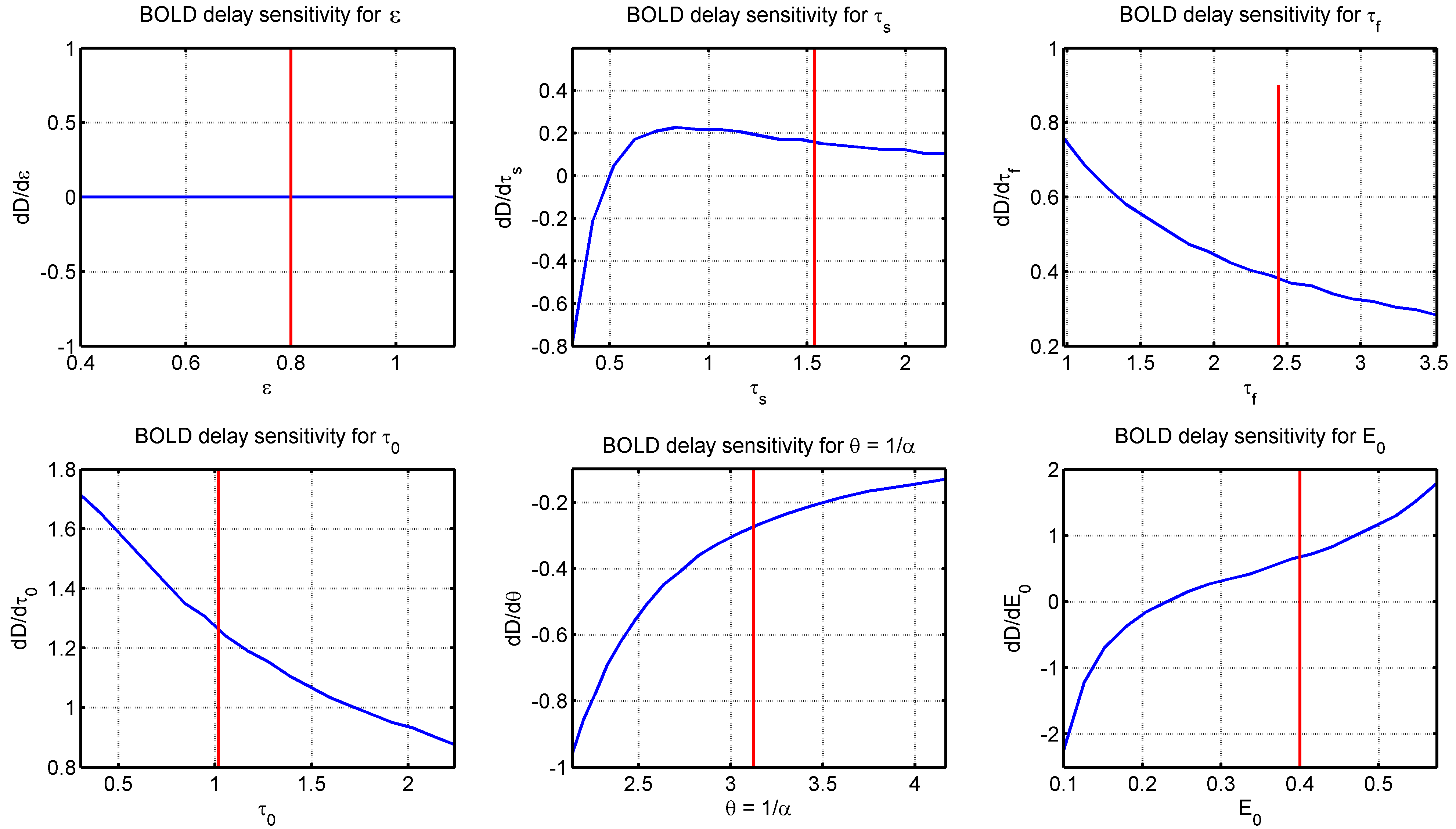
Figure 1: Delay sensitivity analysis for the peak-to-peak time (or delay) $D$ between neuronal activity and BOLD signal for the deterministic model (1)-(4) with $\sigma_{z}=0$ and $\sigma_{y}=0$. For each panel, we vary the corresponding parameter keeping all other parameters fixed to typical values. The blue line indicates the sensitivity $dD/d\omega_{i}$ of the delay for changes in the corresponding parameter $\omega_{i}\in\Omega=(\epsilon,\tau_{s},\tau_{f},\tau_{0},\alpha,E_{0})$. The red vertical lines are the typical values in table 1 and $\tau_{0}=1.02$, $\tau_{f}=2.44$.

Given an input, the hemodynamic parameters $\Omega=(\epsilon,\tau_{s},\tau_{f},\tau_{0},\alpha,E_{0})$ determine the delay between the neuronal activity and the BOLD signal. Similarly, when inverting the system to infer the hidden states and input, the peak of the mean neuronal activity is determined by the hemodynamic parameters. Since the timing of the neuronal peak is a proxy for the input timing, estimating the parameters of the hemodynamic system is crucial.

However, not all parameters have a significant influence on the delay $D=t_{max,B}-t_{max,z}$ defined as the difference between the timing of the peak in the BOLD and neuronal signal $z_{t}$. Given an input to the neuronal system, this influence can be measured by the change in $D$ when a single parameter is varied. To show this influence, we compute–by numerical integration–the sensitivity $dD/d\omega_{i}$ of the delay to changes in the parameter $\omega_{i}\in\Omega$.

Figure 1 shows this sensitivity for each parameter, keeping all other fixed to the typical values in table 1 together with $\tau_{0}=1.02$, $\tau_{f}=2.44$. It is observed that the neuronal efficacy $\epsilon$ has no influence on the delay of the BOLD amplitude and that, in the neighborhood of the typical values, the transit time $\tau_{0}$ has the largest sensitivity (lower left panel), followed by the resting oxygen extraction $E_{0}$ and the auto-regulation $\tau_{f}$.

We can use the forward sensitivity method to estimate the values of hemodynamic parameters given the input and fMRI time series. For simplicity, only two of the three most relevant parameters are considered, namely $\tau_{0}$ and $\tau_{f}$. It turns out that including $E_{0}$ in the learning procedure results in local minima if the initialization is far from the ground truth value of $E_{0}$. This could be an effect of the insensitivity of the system’s output to different parameter sets, as explored in [6]. Hence, the resting oxygen extraction $E_{0}$ as well as all other parameters will be fixed to their typical values.

In what follows, the forward sensitivity method for $\tau_{f}$ and $\tau_{0}$ is analyzed using synthetic data generated as described in section 2.3.1. In figure 2, the parameters are estimated from 10 random initializations. As expected, the estimated parameters are not exactly those of the ground truth, but all initializations converge to the same values close to them (left panels). These parameters minimize the neg. log-likelihood of the data from up to 100 to a value of 23, below that of 24 for the ground truth (in black, bottom right panel).

In case there is enough information in the data–either from precise observations ($\sigma_{obs}=0$) or when the signal is corrupted by noise but observed at very high time resolution ($TR=dt$)–the parameters converge to the ground truth. Consequently, the error between the learned and the ground truth signal is less than $3\times 10^{-8}$ over the entire time interval (not shown).

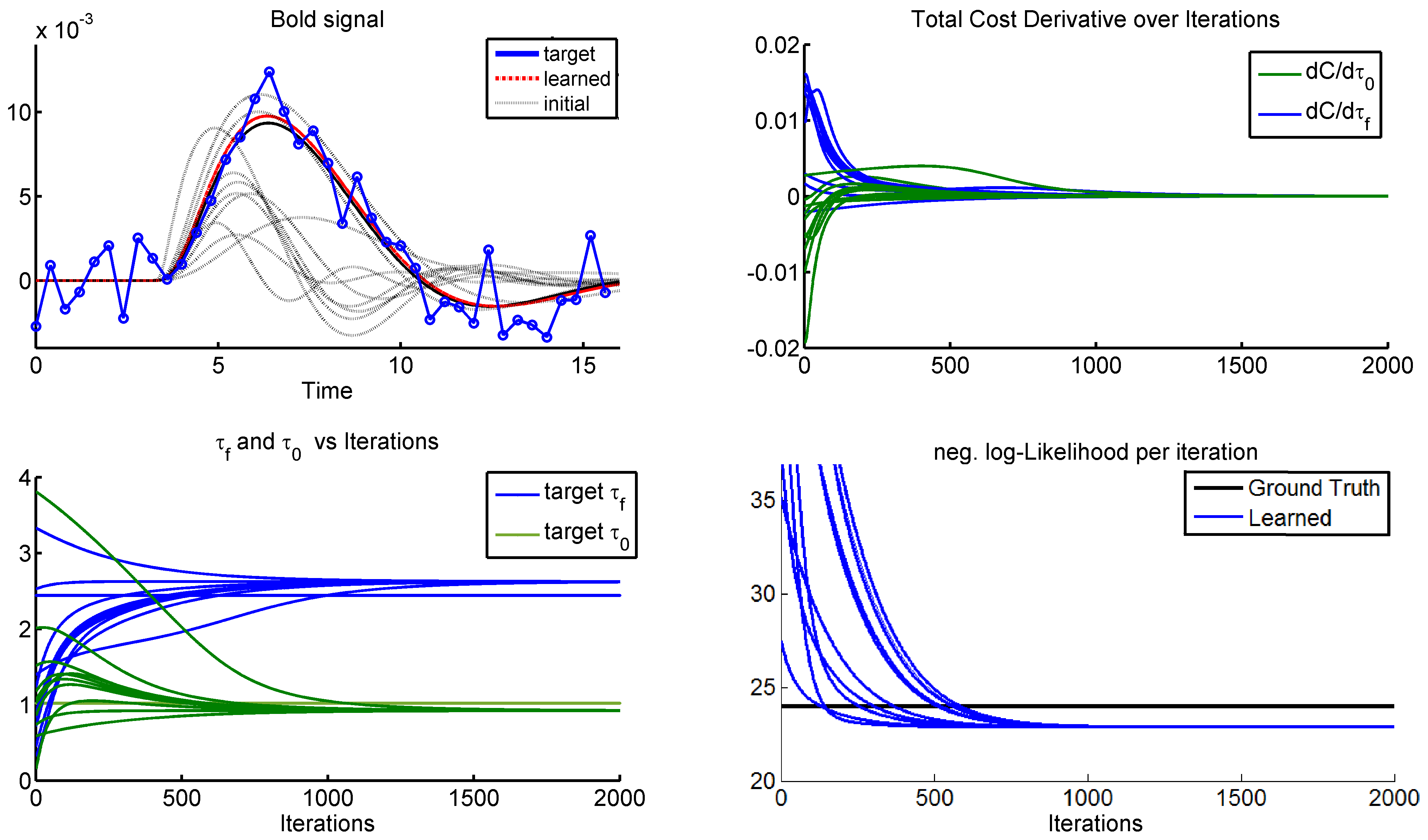
Figure 2: Forward sensitivity learning: sparse noisy observations (Top-Left). The blue markers represent the data sampled. The interval between observations is $TR=0.4$. Notice that, although the ML estimates have some error due to the noisy sparse data, the ML solutions are reliable across a wide range of initializations of the parameters.

Finally, the parameters $\tau_{0}$ and $\tau_{f}$ are estimated for each ROI using the mean time series of the first trial. The results are summarized in table 2. In the analysis using synthetic data, we observe estimates that are close to the ground truth value for small observation noise (not shown). Given that the mean signal over the first trial has little noise, it is expected that learned parameters result in a small error in the input timing of the signals estimated from the second trial.

	A	V	M
$\tau_{0}$	1.75	1.73	2.00
$\tau_{f}$	1.56	2.58	1.32

Table 2: Estimated values of hemodynamic parameters $\tau_{0}$ and $\tau_{f}$. These parameters account for most of the variability in the peak-to-peak delay between the neuronal response and the BOLD signal. The mean signal of the first trial is used to estimate these parameters, which are used in the input timing estimates of the second trial.

3.2 Nonlinear Deconvolution of fMRI Data

3.2.1 Hidden Neuronal Activity

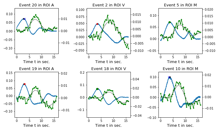
Figure 3: Examples of posterior estimates of neuronal activity (blue) and mean BOLD signal (dashed black). Left axis gives the scale of the neuronal activity $z_{t}$ and the right the scale of the BOLD signal change. The green graphs represent the fMRI time series. The black star indicates the true event timing, while the other markers indicate the estimated input timing from the maximum neuronal activity. The markers are coded according to the stimulus modality: blue cross for auditory (A) stimulus, green dot for visual (V) stimulus and red star for audio-visual stimulus (AV).

APIS is applied individually to the fMRI time series of the second trial. For all estimations, $5\times 10^{4}$ particles are used over 120 iterations to infer the neuronal activity. Unless stated otherwise all simulations use the typical values in table 1, the estimated values in table 2 and the noise level is initialized at $\sigma_{z}=0.3$.

Figure 3 shows typical examples of the posterior estimates using APIS. Each column represents a ROI. The markers show the stimulus time (black star) and the estimated input time. The color of the markers represent the modality of the stimulus presented (A: blue, V: green, AV: red). The neuronal signals (blue line) follow very closely the estimated input due to the short time scale of the system. In addition, they have large amplitudes and a clear peak around the input timing. This gives BOLD signals with high likelihood (black dashed lines).

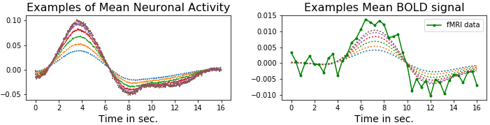
Figure 4: Examples of posterior mean estimates depending on the noise level: from the blue solution with $\sigma_{dyn}=0.44$ to the brown solution with $\sigma_{dyn}=1.17$. The higher the noise $\sigma_{dyn}$, the stronger the inferred input and, thus, the neuronal signal has a larger amplitude (left panel). This gives higher amplitudes in the corresponding mean BOLD signals (right). Nevertheless, the width of the resulting neuronal signals does not change significantly.

The amplitudes of both, the neuronal and the BOLD signals, depend directly on the dynamic noise $\sigma_{dyn}$. In figure 4, examples of the posterior mean estimates of both the neuronal activity and the BOLD signal are shown for a given time series (green lines with markers). The noise $\sigma_{dyn}$ varies from $0.44-1.17$, which result in different mean signals with varying amplitudes, from low to high respectively.

While the maximum of the neuronal activity is a good proxy for the input timing, the time scale of the true input cannot be captured by the inferred signal $u(z_{t},t)$. This is due to the well known low pass-filter characteristic of the hemodynamic transformation, which makes fast variations in the neuronal activity have a minor impact on the resulting BOLD signal. Hence, although the amplitude of the inferred input increases with the noise level, its width of several seconds remains broad regardless of the noise, see left panel on figure 4. These results are robust against changes in the model to have faster time scales, for instance a geometric Brownian motion with a non vanishing diffusion term at the origin, or changes in the time scale $A$ of the neuronal system.

The poor temporal resolution of the neuronal signal resulting from inverting the hemodynamic system is confirmed with a random grid search over the neuronal space at each time point $z_{t}$ to obtain ML-estimates. Using this method the resulting signal is similar to our results; it has also a peak centered around the input and its width is several seconds (not shown). Hence, without explicitly modeling fast changes in the input over time, the deconvolved signal will not reflect fast fluctuations of the inputs.

3.2.2 Comparison with Bootstrap Particle Filter-Smoother

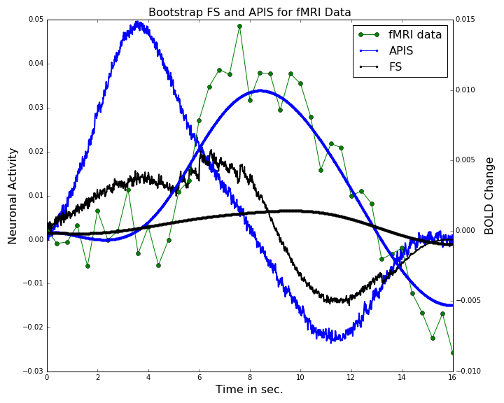
Figure 5: Comparison of APIS vs the vanilla bootstrap filter-smoother (FS). The left y-axis shows the strength of the neuronal activity $z_{t}$, while the right axis the BOLD response change. The jittered lines are the neuronal activity estimates of APIS (blue) and FS (black). The thick continuous lines are their corresponding BOLD response. Notice the low amplitude of the FS estimates. This results in a negative log-likelihood score of 374; much higher than the score for APIS with 97.

In what follows we compare APIS to the vanilla flavor bootstrap particle filter-smoother (FS). The algorithm for FS is implemented as in Lindsten and Schön [30]. We estimate the smoothing distribution over the neuronal activity using 40 workers with $5000$ particles each. The computation of the statistics of the posterior is parallelized across all workers. Since the effective samples of the FS deteriorates for early times, the variance of the estimates at these times is large. For this reason, 100 forward passes on each CPU are performed to obtain better estimates. The noise level $\sigma_{dyn}$ is set to the same value (0.39) as the one estimated by the EM procedure for APIS.

Figure 5 compares the estimates from APIS and FS for event #2 in the V ROI. The result shows that the FS has problems estimating a large, clear amplitude of the neuronal activity due to the strong model mismatch from the lack of input. In contrast, the control drift $u(x_{t},t)$ in APIS accounts for the lack of input in our model, giving a clear peak in the neuronal activity centered at the event time. Scoring both results in terms of the negative log-likelihood, the FS has a much higher score of 374 compared to APIS with 97. Hence, the FS samples represent poorly the data and are bias towards the prior stationary distribution given by the uncontrolled dynamics.

3.2.3 Validation via Input Timing Estimates from Single Event fMRI Time Series

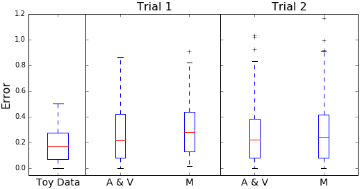
Figure 6: Performance summary of timing estimates for APIS. Synthetic data is used to define a reference empirical distribution of timing errors (left box plot). The hemodynamic model is estimated using trial 1 and trial 2 is used to evaluate the generalization of the deconvolution to unseen data. Although the variation in the inter-quartile range is up to 62% higher than that of the reference distribution, over 75% of the error in both trials lie within the range of the reference distribution and all third quartiles lie around $TR=0.4$. The median values lie within the third quartile of the reference distribution. Notice that the models estimated in trial 1 generalize well in trial 2.

As an indication of the performance of the proposed deconvolution, we consider box plots representing the empirical distribution over errors between the estimated timings and the actual event time. Comparing these distributions with the "reference" empirical distribution obtained from synthetic data gives us an idea of how well the deconvolution procedure, together with the parameter estimates, extracts timing information at the neuronal level.

For the error distribution from synthetic data, we generate 30 time series with the same characteristics of the real data (TR, BOLD change amplitude, trial length, etc) using the same ground truth as in 2.3.1 but with a neuronal noise of $\sigma_{z}=0.01$. To infer the neuronal signals, the same algorithmic parameters are used in synthetic and real data.

Figure 6 shows the box plots for the synthetic data, the combined errors for the sensory ROIs and the errors from the motor ROI in each trial. We consider the sensory regions and the motor region separately because the inputs to the sensory ROIs are exactly the visual and auditory cues, which are known with precision, while the inputs to the motor ROI are less certain. The first box plot on the left side shows that even in the idealized case of having the exact hemodynamic model, the estimated timings have a median error of $0.18$ with an inter-quartile range of $[0.08,0.28]$. This is to be expected due to the noise in the system. The median error in both trials lies between $[0.22,0.28]$ and thus within the third quartile of the reference distribution. Interestingly, the median of the sensory ROIs have very similar values about 23% higher than that of the reference, but the median of the motor ROI is in both trials up to 50% higher. Nevertheless, in all cases more than 75% of the errors lie within the range of the reference distribution and there is an overall count of only 7 outliers. All third quartile values in both trials lie around the TR value.

Although in both trials the variation in the error is about 62% higher than in the reference distribution, we observe consistency between the trials. Hence, the parameters estimated in the first trial generalize well in the second trial. The source of the higher error is probably due to both, a bias in the estimation of the hemodynamic system and a large variance in the data, possibly from the effects of the neuronal noise on the BOLD response, as this can be observed in synthetic data (not shown).

These results show that APIS is capable of extracting timing information with a very high resolution, well beyond the typical time scales of the hemodynamic transformation and the TR. Even more, comparing the error obtained from 2 different trials from the same subject–one used to fit the model–it is possible to assess the generality of the estimated model.

4 Discussion

In this article, the adaptive importance sampler APIS [36] is applied to fMRI data obtained during a reaction time experiment to infer the latent neuronal activity in the visual, auditory and motor ROIs. In addition, APIS is extended by an EM-based procedure to increase the neuronal noise in the system such that signals with high likelihood can be inferred while maintaining the sampler at a fixed efficiency. We show that this procedure is capable of compensating for signals not included in the model to obtain accurate results. In this case, the input to the ROI is disregarded in the reconstruction of the latent neuronal activity and the aim is to obtain accurate absolute timing estimates of the events as a way of validating the method on real fMRI time series. Accuracy is measured in terms of the empirical distribution of the error in input timing estimates compared to a reference distribution obtained from synthetic data given the ground truth model. In addition, our method shows a clear advantage over particle methods in terms of efficiently minimizing the variance of the neural estimates and the negative likelihood.

In some cases, the ML-estimates of the hemodynamic parameters resulted in a higher MSE in the event timing estimates of trial 2. One source of error is a bias in the model caused by a distortion of the mean signal used in training due to outliers in the data. To avoid this effect, it might be wise to consider neuronal noise in the model estimation procedure and obtain ML-estimates for each time series individually. For this, APIS can be merged readily with the Forward Sensitivity method to jointly estimate parameters and hidden states.

Another source of bias in the timing estimates can be caused by a fine-tuning problem where other hemodynamic parameters must be learned. Since the application of the Forward Sensitivity method is cumbersome for larger number of parameters, other possible modifications of the joint estimation procedure exist. For instance, the addition of a small noise signal to the hemodynamic system allows the implementation of the EM algorithm on the full system. In this case, the parameters are updated with the gradient of the state transition density under the posterior statistics. This gives simpler learning rules than the Forward Sensitive method, but it requires the estimation of a control signal for each additional noisy degree of freedom. Nonetheless, APIS has the additional benefit that non-neuronal sources in the hemodynamic response could be detected in a fully controlled setting because, as shown here, hidden signals that are not modeled can be captured by the controller. An additional advantage, albeit the higher computational effort required, is the better behavior of the effective sample size, which is higher and less sensible to changes in the neuronal noise. In this work, however, we consider only a 1-dimensional linear feedback controller for simplicity.

Interesting parallels to our case study are found in [18] and more recently [39]. In the former, toy data was used to analyze their proposed method for short stimuli of about $200\ ms$. Interestingly, the cubature Kalman Filter-Smoother (SCKS) presented there obtained similar broad neuronal signals, but there was no report on the accuracy of the input timing estimates. In the latter article, a non-parametric approach was used to asses the susceptibility of the SCKS to over-fit the data. Both methods were applied to fMRI time series obtained during the presentation of visual stimuli with a duration of 2 s. In this case too, the SCKS estimates had clear peaks in the neuronal response around the stimulus timing, but the stimulus duration was one order of magnitude larger than in our case study and there was no report on precise input timing estimates. Hence, these methods were tested in a different dynamic regime of the hemodynamic transformation than here. On the contrary, in our case study both aspects–short stimuli and real fMRI data–are combined.

The lack of direct measurements of the neuronal activity makes it difficult to asses the quality of any estimation, but the theoretical derivation of APIS ensures the optimality of the posterior estimates given the model and a sufficiently high number of effective samples. Although we recognize the need to compare our proposed method with interesting alternatives, a fair comparison is difficult because the accuracy of the different methods in different dynamic regimes is not known and there is no ground truth available. Thus, it is important to clarify which of the available methods are good approximations for the different stimuli modalities and dynamic regimes of the nonlinear hemodynamic system, and how they compare to our adaptive importance sampling method, which is applicable in any dynamic regime. Hence, finding good benchmarks for all methods with many types of stimulus modalities is urgently needed and an extensive comparison of alternative methods should be addressed in future work. In this analysis, the question of how accurate the Gaussian approximations are in the different dynamic regimes would require special attention.

To overcome the lack of a ground truth, the proposed method was validated by its ability to directly extract timing information out of the time series. Inferring the timing of a stimulus shorter than the TR of the acquisition requires very precise estimations of the neuronal activity, especially if very fast changes are suppressed by the hemodynamic transformation and the only retrievable information are signals with a temporal resolution an order of magnitude larger. Hence, we believe that the proposed analysis can serve as a benchmark on the precision of timing information retrieval for deconvolution methods of fMRI time series.

Finally, the proposed method can accommodate any nonlinear model that can be formulated as a stochastic differential equation, for instance the recent model [19]. Moreover, the model can be easily extended to accommodate context dependent connectivity and other confound signals like heart rate or head motion. This generality and flexibility together with the demonstrated accuracy and efficiency makes the proposed method an interesting alternative to other nonlinear deconvolution methods for event related and resting state fMRI data.

Acknowledgments

The work of HC Ruiz Euler was supported by the European Commission through the FP7 Marie Curie Initial Training Network 289146, NETT: Neural Engineering Transformative Technologies.

References

- Birn et al. [2001] Rasmus M Birn, Ziad S Saad, and Peter A Bandettini. Spatial heterogeneity of the nonlinear dynamics in the fmri bold response. Neuroimage, 14(4):817–826, 2001.
- Briers et al. [2010] Mark Briers, Arnaud Doucet, and Simon Maskell. Smoothing algorithms for state–space models. Annals of the Institute of Statistical Mathematics, 62(1):61–89, 2010.
- Buxton et al. [1998] Richard B Buxton, Eric C Wong, and Lawrence R Frank. Dynamics of blood flow and oxygenation changes during brain activation: the balloon model. Magnetic resonance in medicine, 39(6):855–864, 1998.
- Daunizeau et al. [2009] Jean Daunizeau, Karl J Friston, and Stefan J Kiebel. Variational bayesian identification and prediction of stochastic nonlinear dynamic causal models. Physica D: Nonlinear Phenomena, 238(21):2089–2118, 2009.
- David et al. [2008] Olivier David, Isabelle Guillemain, Sandrine Saillet, Sebastien Reyt, Colin Deransart, Christoph Segebarth, and Antoine Depaulis. Identifying neural drivers with functional mri: an electrophysiological validation. PLoS biology, 6(12):e315, 2008.
- Deneux and Faugeras [2006] Thomas Deneux and Olivier Faugeras. Using nonlinear models in fmri data analysis: model selection and activation detection. NeuroImage, 32(4):1669–1689, 2006.
- Douc et al. [2011] Randal Douc, Aurélien Garivier, Eric Moulines, and Jimmy Olsson. Sequential monte carlo smoothing for general state space hidden markov models. The Annals of Applied Probability, 21(6):2109–2145, Dec 2011. ISSN 1050-5164. doi: 10.1214/10-AAP735. URL http://projecteuclid.org/euclid.aoap/1322057317.
- Fleming and Mitter [1982] Wendell H Fleming and Sanjoy K Mitter. Optimal control and nonlinear filtering for nondegenerate diffusion processes. Stochastics: An International Journal of Probability and Stochastic Processes, 8(1):63–77, 1982.
- Formisano and Goebel [2003] Elia Formisano and Rainer Goebel. Tracking cognitive processes with functional mri mental chronometry. Current opinion in neurobiology, 13(2):174–181, 2003.
- Friston et al. [2010] Karl Friston, Klaas Stephan, Baojuan Li, and Jean Daunizeau. Generalised filtering. Mathematical Problems in Engineering, 2010, 2010.
- Friston [2008] Karl J Friston. Variational filtering. NeuroImage, 41(3):747–766, 2008.
- Friston et al. [1998a] Karl J Friston, P Fletcher, Oliver Josephs, ANDREW Holmes, MD Rugg, and Robert Turner. Event-related fmri: characterizing differential responses. Neuroimage, 7(1):30–40, 1998a.
- Friston et al. [1998b] Karl J Friston, Oliver Josephs, Geraint Rees, and Robert Turner. Nonlinear event-related responses in fmri. Magnetic resonance in medicine, 39(1):41–52, 1998b.
- Friston et al. [2000] Karl J Friston, Andrea Mechelli, Robert Turner, and Cathy J Price. Nonlinear responses in fmri: the balloon model, volterra kernels, and other hemodynamics. NeuroImage, 12(4):466–477, 2000.
- Friston et al. [2003] Karl J Friston, Lee Harrison, and Will Penny. Dynamic causal modelling. Neuroimage, 19(4):1273–1302, 2003.
- Friston et al. [2008] Karl J Friston, N Trujillo-Barreto, and Jean Daunizeau. Dem: a variational treatment of dynamic systems. Neuroimage, 41(3):849–885, 2008.
- Griffanti et al. [2017] Ludovica Griffanti, Gwenaëlle Douaud, Janine Bijsterbosch, Stefania Evangelisti, Fidel Alfaro-Almagro, Matthew F Glasser, Eugene P Duff, Sean Fitzgibbon, Robert Westphal, Davide Carone, et al. Hand classification of fmri ica noise components. NeuroImage, 154:188–205, 2017.
- Havlicek et al. [2011] Martin Havlicek, Karl J Friston, Jiri Jan, Milan Brazdil, and Vince D Calhoun. Dynamic modeling of neuronal responses in fmri using cubature kalman filtering. NeuroImage, 56(4):2109–2128, 2011.
- Havlicek et al. [2015] Martin Havlicek, Alard Roebroeck, Karl Friston, Anna Gardumi, Dimo Ivanov, and Kamil Uludag. Physiologically informed dynamic causal modeling of fmri data. NeuroImage, 122:355–372, 2015.
- Jimenez and Ozaki [2003] JC Jimenez and T Ozaki. Local linearization filters for non-linear continuous-discrete state space models with multiplicative noise. International Journal of Control, 76(12):1159–1170, 2003.
- Johnston et al. [2008] Leigh A Johnston, Eugene Duff, Iven Mareels, and Gary F Egan. Nonlinear estimation of the bold signal. NeuroImage, 40(2):504–514, 2008.
- Kappen [2005] Hilbert J Kappen. Linear theory for control of nonlinear stochastic systems. Physical review letters, 95(20):200201, 2005.
- Kappen [2011] Hilbert J Kappen. Optimal control theory and the linear bellman equation. Inference and Learning in Dynamic Models, pages 363–387, 2011.
- Kappen et al. [2012] Hilbert J Kappen, Vicenç Gómez, and Manfred Opper. Optimal control as a graphical model inference problem. Machine learning, 87(2):159–182, 2012.
- Kappen and Ruiz [2016] Hilbert Johan Kappen and Hans Christian Ruiz. Adaptive importance sampling for control and inference. Journal of Statistical Physics, 162(5):1244–1266, 2016.
- Katwal et al. [2013] Santosh B Katwal, John C Gore, J Christopher Gatenby, and Baxter P Rogers. Measuring relative timings of brain activities using fmri. NeuroImage, 66:436–448, 2013.
- Li et al. [2011] Baojuan Li, Jean Daunizeau, Klaas E Stephan, Will Penny, Dewen Hu, and Karl Friston. Generalised filtering and stochastic dcm for fmri. neuroimage, 58(2):442–457, 2011.
- Liao et al. [2002] Chien Heng Liao, Keith J Worsley, J-B Poline, John AD Aston, Gary H Duncan, and Alan C Evans. Estimating the delay of the fmri response. NeuroImage, 16(3):593–606, 2002.
- Lindquist [2008] Martin A Lindquist. The statistical analysis of fmri data. Statistical Science, pages 439–464, 2008.
- Lindsten and Schön [2013] Fredrik Lindsten and Thomas B Schön. Backward simulation methods for monte carlo statistical inference. Foundations and Trends in Machine Learning, 6(1):1–143, 2013.
- Miezin et al. [2000] Francis M Miezin, L Maccotta, JM Ollinger, SE Petersen, and RL Buckner. Characterizing the hemodynamic response: effects of presentation rate, sampling procedure, and the possibility of ordering brain activity based on relative timing. Neuroimage, 11(6):735–759, 2000.
- Murray and Storkey [2011] Lawrence Murray and Amos Storkey. Particle smoothing in continuous time: A fast approach via density estimation. Signal Processing, IEEE Transactions on, 59(3):1017–1026, 2011.
- Narsude et al. [2015] Mayur Narsude, Daniel Gallichan, Wietske Van Der Zwaag, Rolf Gruetter, and José P Marques. Three-dimensional echo planar imaging with controlled aliasing: A sequence for high temporal resolution functional mri. Magnetic resonance in medicine, 2015.
- Riera et al. [2004] Jorge J Riera, Jobu Watanabe, Iwata Kazuki, Miura Naoki, Eduardo Aubert, Tohru Ozaki, and Ryuta Kawashima. A state-space model of the hemodynamic approach: nonlinear filtering of bold signals. NeuroImage, 21(2):547–567, 2004.
- Roweis and Ghahramani [2001] Sam Roweis and Zoubin Ghahramani. Learning nonlinear dynamical systems using the expectation–maximization algorithm. Kalman filtering and neural networks, 6:175–220, 2001.
- Ruiz and Kappen [2017] Hans-Christian Ruiz and Hilbert J Kappen. Particle smoothing for hidden diffusion processes: Adaptive path integral smoother. IEEE Transactions on Signal Processing, 65(12):3191–3203, 2017.
- Sengupta et al. [2014] Biswa Sengupta, Karl J Friston, and William D Penny. Efficient gradient computation for dynamical models. NeuroImage, 98:521–527, 2014.
- Smith et al. [2011] Stephen M Smith, Karla L Miller, Gholamreza Salimi-Khorshidi, Matthew Webster, Christian F Beckmann, Thomas E Nichols, Joseph D Ramsey, and Mark W Woolrich. Network modelling methods for fmri. Neuroimage, 54(2):875–891, 2011.
- Sreenivasan et al. [2015] Karthik Ramakrishnan Sreenivasan, Martin Havlicek, and Gopikrishna Deshpande. Nonparametric hemodynamic deconvolution of fmri using homomorphic filtering. IEEE transactions on medical imaging, 34(5):1155–1163, 2015.
- Stephan et al. [2008] Klaas Enno Stephan, Lars Kasper, Lee M Harrison, Jean Daunizeau, Hanneke EM den Ouden, Michael Breakspear, and Karl J Friston. Nonlinear dynamic causal models for fmri. Neuroimage, 42(2):649–662, 2008.
- Wager et al. [2005] Tor D Wager, Alberto Vazquez, Luis Hernandez, and Douglas C Noll. Accounting for nonlinear bold effects in fmri: parameter estimates and a model for prediction in rapid event-related studies. NeuroImage, 25(1):206–218, 2005.