Diagrammatic treatment of few-photon scattering
from a Rydberg blockaded atomic ensemble in a cavity

Abstract

In a previous letter (Grankin et al., 2016) we studied the giant optical nonlinearities of a Rydberg atomic medium within an optical cavity, in the Schwinger-Keldysh formalism. In particular, we calculated the non-linear contributions to the spectrum of the light transmitted through the cavity. In this article we spell out the essential details of this calculation, and we show how it can be extended to higher input photon numbers, and higher order correlation functions. As a relevant example, we calculate and discuss the three-photon correlation function of the transmitted light, and discuss its physical significance in terms of the polariton energy levels of the Rydberg medium within the optical cavity.

I Introduction

Optical quantum information processing requires photonic gates, that may be implemented either deterministically or non-deterministically (Nielsen and Chuang, 2010). For the sake of efficiency and scalability it is preferable to implement them in a deterministic way, which requires photon-photon interactions. Though impossible to achieve directly, such interactions can be effectively emulated by coupling photons to a medium with a “giant” optical non-linearity, i.e. large enough to allow photonic qubits to interact. In this article we study an example of such a medium, consisting in an atomic ensemble driven in a configuration of electromagnetically induced transparency (EIT), involving a highly excited Rydberg level. Following this approach, few-photon non-linearities were achieved in free-space configuration setups: antibunching of photons was observed in dispersive (Firstenberg et al., 2013) and absorptive regimes (Peyronel et al., 2012), photon switches/transistors were implemented (Gorniaczyk et al., 2014; Tiarks et al., 2014) and photon blockade was demonstrated (Dudin and Kuzmich, 2012; Maxwell et al., 2013). By placing such a medium in an optical cavity, strong nonlinearities for classical light were predicted and demonstrated (Grankin et al., 2014, 2015), as well as quantum effects (Boddeda et al., 2016; Parigi et al., 2012; Stanojevic et al., 2013) recently observed (Jia et al., 2017). Such a non-linear medium is actually a strongly correlated many-body system, and its full dynamics as well as its effects on the incoming photons cannot be computed exactly. So far, analytic expressions of dynamical variables like, the correlation functions of the transmitted field could be derived either using ad hoc models – such as the Rydberg bubble picture (Petrosyan et al., 2011; Gorshkov et al., 2013), or resorting to the perturbation theory restricted to the lowest non-vanishing order in the number of incoming photons (Grankin et al., 2015; Gorshkov et al., 2011).

In this article, we employ the Schwinger-Keldysh contour formalism (Schwinger, 1961; Rammer, 2007; Stefanucci and van Leeuwen, 2013) to derive analytic expressions for field correlation functions for a Rydberg-EIT medium within an optical cavity, beyond the lowest non-vanishing order in the excitation number (Grankin et al., 2015). By opening a systematic and manageable way to deal with higher-order terms, our approach breaks new ground for solving the outstanding problem set by the many-body dynamics of Rydberg-blockaded ensembles interacting with quantized light. It also allows us to unveil nontrivial physical features of the transmitted light spectrum that we explain by a simple polaritonic picture. Finally, it is important to notice that parameters used for simulations correspond to experimental setups such as the one used in (Jia et al., 2017), or in (Parigi et al., 2012; Boddeda et al., 2016) with an upgraded cavity. Therefore, the effects predicted by our model can be, in principle, experimentally observed.

The purpose of this article is to present the calculation of photon-photon correlation functions using the formalism quoted above. For all physical quantities of interest, we will perform the expansion and full resummation, for the first few orders in the cavity feeding rate. In Sec. II we introduce the model and notations, and in Sec. III we present the elements of the Schwinger-Keldysh formalism that are useful for our purpose. In Sec. IV we derive the first-order averages for cavity and atomic variables, and in Sec. V we analytically derive the the photonic pair correlation in the lowest non-vanishing order. In Sec. VI we go beyond the lowest order and derive the analytic expression of the transmission spectrum of the cavity, distinguishing its elastic and inelastic parts. We give a physical explanation to the inelastic part using a simple polaritonic picture. In the last section, we derive the third-order correlation function of the transmitted light by adopting the approach developed by L. D. Faddeev in application to the quantum-mechanical three-body scattering problem. We get thus new results about three-photon correlation functions, that are discussed from a physical point of view.

II Model and notations

Coupled atom-cavity system

We consider an ensemble of $N$ atoms with a ground, intermediate and Rydberg states, denoted by $\left|g\right\rangle$, $\left|e\right\rangle$ and $\left|r\right\rangle$, respectively, loaded in an optical cavity (Grankin et al., 2014) (see Fig. 1). The transitions $g\leftrightarrow e$ and $e\leftrightarrow r$ are respectively driven by the cavity mode, of frequency $\omega_{c}$ and annihilation operator $a$, and the strong control field, with the coupling strength $g$ and the Rabi frequency $\Omega_{cf}$, respectively. The cavity is fed through an input mirror with decay rate $\gamma_{c}^{\left(f\right)}$ by a weak probe laser of frequency $\omega_{p}$, while the field transmitted by the cavity can be detected through an output mirror with decay rate $\gamma_{c}^{\left(d\right)}$; we moreover set $\gamma_{c}\equiv\gamma_{c}^{\left(f\right)}+\gamma_{c}^{\left(d\right)}$. We define detunings for the cavity $\Delta_{c}=\left(\omega_{p}-\omega_{c}\right)$, single-photon $\Delta_{e}=\left(\omega_{p}-\omega_{eg}\right)$ and two-photon $\Delta_{r}=\left(\omega_{p}+\omega_{cf}-\omega_{rg}\right)$, with respect to the frequencies $\omega_{eg}$ and $\omega_{rg}$ of the $g\leftrightarrow e$ and $g\leftrightarrow r$ transitions. We denote by $\gamma_{e}$ and $\gamma_{r}$ the decay rates from the intermediate $\left|e\right\rangle$ and Rydberg $\left|r\right\rangle$ states, respectively.

If there were no atomic interactions, the cloud driven under perfect EIT conditions $\left(\gamma_{r}\approx\Delta_{r}\approx 0\right)$, would be transparent for the probe light (Fleischhauer and Lukin, 2000). The dipole-dipole-interaction-induced blockade phenomenon (Saffman et al., 2010; Lukin et al., 2001) actually prevents most of the atoms in the sample from being Rydberg excited. If $\Delta_{e}\approx 0$, spontaneous emission from the intermediate state is strongly enhanced which significantly modifies the shape of the transmitted light spectrum. This effect can be characterized by the steady state correlation function of the intracavity light $\left\langle a^{\dagger}\left(t\right)a\left(0\right)\right\rangle$ (Walls and Milburn, 2007). At the lowest non-vanishing order in the feeding rate $\left|\alpha\right|\equiv\sqrt{2\gamma_{c}^{\left(f\right)}I_{in}}$, where $I_{in}$ is the incident photon flux fed into the cavity, the correlation function was shown to factorize, i.e. $\left\langle a^{\dagger}\left(t\right)a\left(0\right)\right\rangle^{\left(2\right)}=\left\langle a^{\dagger}\left(t\right)\right\rangle^{\left(1\right)}\left\langle a\left(0\right)\right\rangle^{\left(1\right)}$ (Grankin et al., 2015), where the superscript denotes the order in $\alpha$. To reveal nonlinear features, one has to investigate orders higher than four – by conservation of excitation number the third order vanishes. Usual techniques are not suited to this task. In particular, the standard fourth-order perturbative expansion would already lead to a cumbersome hierarchy of Heisenberg equations which could hardly be generalized further. Here, we show that the Schwinger-Keldysh contour formalism (Schwinger, 1961; Rammer, 2007; Stefanucci and van Leeuwen, 2013) allows one to compute dynamical variables of the system up to a priori arbitrary order in the feeding strength, in a systematic and handy way. Besides bringing physical insight into the specific problem considered here, our calculation demonstrates how powerful this approach is to deal with non-equilibrium dynamics of atomic systems as already stressed in (Fleischhauer and Yelin, 1999).

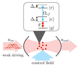
Figure 1: Atomic level scheme and the setup.

Dynamical equations of the system.

According to Holstein-Primakoff approximation, the atomic lowering operators $\sigma_{ge}^{\left(n\right)}$ and $\sigma_{gr}^{\left(n\right)}$ can be treated as bosons $b_{n}$ and $c_{n}$, respectively, in the low excitation regime (Grankin et al., 2015; Bienias et al., 2014). The intrinsic (saturation) nonlinearity of the EIT ladder scheme (for the probe beam) is neglected from our consideration as it is much smaller than the nonlinear effects induced by Rydberg interactions, for the chosen regime of parameters. The Hamiltonian of the full system writes $H=H_{0}+H_{int}$ where

$$H_{0} =H_{at}+V_{a-c}+H_{bath}+V_{cav-bath}+V_{at-bath}$$

$$H_{int} =H_{dd}+H_{f}$$

$$H_{dd} =\frac{1}{2}\sum_{m,n}^{N}\kappa_{mn}c_{m}^{\dagger}c_{n}^{\dagger}c_{m}c_{n}$$

$$H_{f} =\alpha\left(a+a^{\dagger}\right)$$

$$H_{at}= \sum_{n=1}^{N}\left\{-\Delta_{e}b_{n}^{\dagger}b_{n}-\Delta_{r}c_{n}^{\dagger}c_{n}+\frac{\Omega_{cf}}{2}\left(b_{n}^{\dagger}c_{n}+b_{n}c_{n}^{\dagger}\right)\right\}$$

$$V_{a-c}= \sum_{n=1}^{N}g\left(ab_{n}^{\dagger}+a^{\dagger}b_{n}\right)-\Delta_{c}a^{\dagger}a$$

where $\kappa_{mn}\equiv C_{6}/\left|\vec{r}_{m}-\vec{r}_{n}\right|^{6}$ denotes the van der Waals interaction potential. Performing the rotating wave and Markov approximations, the relevant Heisenberg-Langevin equations are

$$\frac{d}{dt}a = -\Gamma_{c}a-i\alpha-igb_{n}+\sqrt{2\gamma_{c}^{\left(f\right)}}a_{in}^{\left(f\right)}+\sqrt{2\gamma_{c}^{\left(d\right)}}a_{in}^{\left(d\right)}$$ (1)

$$\frac{d}{dt}b_{n} = -\Gamma_{e}b_{n}-iga-i\frac{\Omega_{cf}}{2}c_{n}+b_{in,n}$$ (2)

$$\frac{d}{dt}c_{n} = -\Gamma_{r}c_{n}-i\frac{\Omega_{cf}}{2}b_{n}-i\sum_{m}\kappa_{m,n}c_{m}^{\dagger}c_{m}c_{n}+c_{in,n}$$ (3)

where $\left\{a_{in}^{\left(f\right)},\;a_{in}^{\left(d\right)},\;b_{in,n},\;c_{in,n}\right\}$ denote the respective Langevin forces associated to the incoming fields from the feeding and detection sides, and to the atomic operators $b_{n}$ and $c_{n}$. We use complex decay rates $\Gamma_{\nu}\equiv\gamma_{\nu}+i\Delta_{\nu}$ where $\nu=c,e,r$ for simplicity.

III Schwinger-Keldysh formalism

III.1 Contour-ordered representation of correlation functions

Throughout this paper, we will focus on evaluating correlation functions of the light transmitted through the cavity, which can be experimentally obtained via multitime measurements of the light outgoing from the setup. Input-output theory shows that, under Markov approximation, these functions simply relate to the intracavity field correlation functions, themselves coupled to the atomic correlation functions via Heisenberg-Langevin equations. The generic form for such correlation functions is

$$\left\langle\widetilde{\mathcal{T}}\left\{\prod_{i=1}^{r}{\cal O}_{H,i}^{\dagger}\left(t_{i}\right)\right\}\mathcal{T}\left\{\prod_{j=r+1}^{r+s}{\cal O}_{H,j}\left(t_{j}\right)\right\}\right\rangle$$ (4)

where ${\cal O}_{H,i}\left(t\right)\equiv e^{{\rm i}H\left(t-t_{0}\right)}{\cal O}_{i}e^{-{\rm i}H\left(t-t_{0}\right)}$ is an arbitrary operator of our system, expressed in the Heisenberg picture with respect to the Hamiltonian $H$ given in the previous subsection. In (4) $\mathcal{T}$ and $\mathcal{\tilde{T}}$ stand for the usual chronological and anti-chronological time-ordering operators, respectively. We also notice that averaging in Eq. (4) is performed over the initial state of the system (i.e. at $t=t_{0}$), that we assume to be the vacuum $\rho_{0}=\left|\textrm{\O}\right\rangle\left\langle\textrm{\O}\right|$ ( i.e. $\left\langle\cdots\right\rangle\equiv{\rm Tr}\left[\rho_{0}\cdots\right]$ ).

Using the relation

$$\mathcal{O}_{H}\left(t\right) = \mathcal{\widetilde{T}}\left\{e^{-i\,\int_{t}^{t_{0}}dsH_{int}\left(s\right)}\right\}\mathcal{O}_{H_{0}}\left(t\right){\cal T}\left\{e^{-i\,\int_{t_{0}}^{t}dsH_{int}\left(s\right)}\right\}$$ (5)

where $H_{int}\left(t\right)\equiv e^{i\,H_{0}\left(t-t_{0}\right)}H_{int}e^{-i\,H_{0}\left(t-t_{0}\right)}$ we get:

$$\left\langle\mathcal{\widetilde{T}}\left\{\prod_{i=1}^{r}{\cal O}_{H,i}^{\dagger}\left(t_{i}\right)\right\}\mathcal{T}\left\{\prod_{j=r+1}^{r+s}{\cal O}_{H,j}\left(t_{j}\right)\right\}\right\rangle$$ (6)

$$= {\rm Tr}\left[\begin{array}[]{c}\rho_{0}\widetilde{\mathcal{T}}\left\{{\cal O}_{H_{0},1}^{\dagger}\left(t_{1}\right)\ldots{\cal O}_{H_{0},r}^{\dagger}\left(t_{r}\right)e^{-i\,\int_{+\infty}^{-\infty}dsH_{int}\left(s\right)}\right\}\\ \times\mathcal{T}\left\{{\cal O}_{H_{0},r+1}\left(t_{r+1}\right)\ldots{\cal O}_{H_{0},r+s}\left(t_{r+s}\right)e^{-i\,\int_{-\infty}^{+\infty}dsH_{int}\left(s\right)}\right\}\end{array}\right]$$ (9)

The form of Eq. (6) suggests to introduce a new variable, which does not merely follow the real axis $\left(-\infty,\infty\right)$ but rather a contour $\mathcal{C}$ made of two branches $\mathcal{C}_{+}=\left(-\infty,+\infty\right)$ and $\mathcal{C}_{-}=\left(+\infty,-\infty\right)$ (Fig. 1). A contour-ordering operator $\mathcal{T_{C}}$ can be defined, accordingly, by

$$\mathcal{T}_{{\cal C}}\left\{A\left(z_{1}\right)B\left(z_{2}\right)\right\}=\begin{cases}A\left(z_{1}\right)B\left(z_{2}\right);&\text{if}\,\,z_{1}\epsilon\mathcal{C}_{-},z_{2}\epsilon\mathcal{C}_{+}\\ B\left(z_{2}\right)A\left(z_{1}\right);&\text{if}\,\,z_{1}\epsilon\mathcal{C}_{+},z_{2}\epsilon\mathcal{C}_{-}\\ \mathcal{T}\left\{\,A\left(z_{1}\right)B\left(z_{2}\right)\,\right\};&\text{if}\,\,z_{1}\epsilon\mathcal{C}_{+},z_{2}\epsilon\mathcal{C}_{+}\\ \tilde{\mathcal{T}}\left\{\,A\left(z_{1}\right)B\left(z_{2}\right)\,\right\};&\text{if}\,\,z_{1}\epsilon\mathcal{C}_{-},z_{2}\epsilon\mathcal{C}_{-}\end{cases}$$

Finally, introducing the notation $\mathcal{O}_{\pm}\left(t\right)\equiv\mathcal{O}_{H_{0}}$$\left(t\,\epsilon\,\mathcal{C}_{\pm}\right)$, we may rewrite Eq. (6) under the form:

$$\left\langle\mathcal{\tilde{T}}\left\{\prod_{i=1}^{r}{\cal O}_{H,i}^{\dagger}\left(t_{i}\right)\right\}\mathcal{T}\left\{\prod_{j=r+1}^{r+s}{\cal O}_{H,j}\left(t_{j}\right)\right\}\right\rangle = \left\langle\mathcal{T_{C}}\left\{\prod_{i=1}^{r}\prod_{j=r+1}^{r+s}{\cal O}_{-,i}^{\dagger}\left(t_{i}\right){\cal O}_{+,j}\left(t_{j}\right)e^{-{\rm i}\int_{{\cal C}}dsH_{int}\left(s\right)}\right\}\right\rangle$$ (10)

For future reference, we expand Eq. (10) with respect to $H_{f}$ and introduce the operator

$$A_{q}\equiv\frac{1}{\sqrt{2\pi}}\int_{-\infty}^{\infty}\left(a_{+}-a_{-}\right)ds$$ (11)

in Eq. (10), where the $q$ subscript stands for the so-called “quantum” variable (Kamenev, 2011):

$$\left\langle{\cal T}_{{\cal C}}\left\{e^{-\mathrm{i}\left(\int_{{\cal C}}H_{dd}\right)-\mathrm{i}\sqrt{2\pi}\alpha\left(A_{q}+A_{q}^{\dagger}\right)}\prod_{i=1}^{r}{\cal O}_{-,i}^{\dagger}\left(t_{i}\right)\prod_{j=r+1}^{r+s}{\cal O}_{+,j}\left(t_{j}\right)\right\}\right\rangle$$ (12)

$$= \sum_{n,k,p}\frac{\left(-\mathrm{i}\sqrt{2\pi}\alpha\right)^{n}}{\left(n-k\right)!k!}\left\langle{\cal T}_{{\cal C}}\left\{\frac{\left(-i\int_{{\cal C}}H_{dd}\right)^{p}}{p!}A_{q}^{n-k}A_{q}^{\dagger k}\prod_{i=1}^{r}\prod_{j=r+1}^{r+s}{\cal O}_{-,i}^{\dagger}\left(t_{i}\right){\cal O}_{+,j}\left(t_{j}\right)\right\}\right\rangle$$

where we used the fact that all operators behave as c-numbers inside a ${\cal T}_{{\cal C}}$-ordered product.

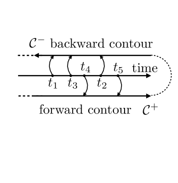
Figure 2: Representation of contour-ordering for the multitime correlation function $\left\langle\tilde{\mathcal{T}}\left\{\mathcal{O}^{1}\left(t_{1}\right)\mathcal{O}^{2}\left(t_{2}\right)\mathcal{O}^{3}\left(t_{3}\right)\right\}\mathcal{T}\left\{\mathcal{O}^{4}\left(t_{4}\right)\mathcal{O}^{5}\left(t_{5}\right)\right\}\right\rangle$.

The generic term of the double perturbative expansion in Eq. (12) is an expectation value in the vacuum state $\rho_{0}$ of a contour-ordered string of creation and annihilation operators

$${\cal S}=\left\langle{\cal T}_{{\cal C}}\left\{e_{p+q}^{\dagger}\left(z_{p+q}\right)\ldots e_{p+1}^{\dagger}\left(z_{p+1}\right)e_{p}\left(z_{p}\right)\ldots e_{1}\left(z_{1}\right)\right\}\right\rangle$$ (13)

where $e_{1},e_{2},\cdots,e_{p+q}$ are bosonic annihilation operators in the interaction picture with respect to $H_{0}$. Applied to our system, Wick’s theorem (Stefanucci and van Leeuwen, 2013; Abrikosov et al., 1975) states that such a contour-ordered string can be decomposed into a sum over all possible pairwise products of creation and annihilation operators in the string in Eq. (13)

$${\cal S}=\sum_{a.p.p}\prod_{k,l}\left\langle{\cal T}_{{\cal C}}\left\{e_{l}\left(z_{l}\right)e_{k}^{\dagger}\left(z_{k}\right)\right\}\right\rangle$$ (14)

The quantity $G_{e_{k}e_{l}}^{\left({\cal C}\right)}\left(z_{l},z_{k}\right)=-{\rm i}\left\langle{\cal T_{C}}\left\{e_{l}\left(z_{l}\right)e_{k}^{\dagger}\left(z_{k}\right)\right\}\right\rangle$ is called the unperturbed contour-ordered Green’s function for the operators $e_{k}$ and $e_{l}$.

Before evaluating the unperturbed Green’s functions, it is important to notice that an implicit part of the theorem’s statement is that the number of creation and annihilation operators should be equal. In the general formula Eq. (12) there are $k+r+2p$ creation operators (recalling that $H_{dd}=\frac{1}{2}\sum_{ij}\kappa_{ij}c_{i}^{\dagger}c_{j}^{\dagger}c_{i}c_{j}$) and $n-k+s+2p$ annihilation operators: the series Eq. (12) should be restricted to the terms which satisfy $k+r+2p=n-k+s+2p$, or equivalently $k=\frac{n+s-r}{2}$. Defining $D=s-r$ we finally have

$$\left\langle\mathcal{T}_{{\cal C}}\left\{\prod_{i=1}^{r}\prod_{j=r+1}^{r+s}{\cal O}_{H,i}^{\dagger}\left(t_{i}\right){\cal O}_{H,j}\left(t_{j}\right)\right\}\right\rangle$$ (15)

$$=\sum_{n:\frac{n+D}{2}\epsilon\mathbb{Z},p}\frac{\left(-\mathrm{i}\sqrt{2\pi}\alpha\right)^{n}}{\left(\frac{n+D}{2}\right)!\left(\frac{n-D}{2}\right)!}\left\langle{\cal T}_{{\cal C}}\left\{\frac{\left(-\mathrm{i}\int_{{\cal C}}H_{dd}\right)^{p}}{p!}A_{q}^{\frac{n-D}{2}}A_{q}^{\dagger\frac{n+D}{2}}\prod_{i=1}^{r}\prod_{j=r+1}^{r+s}{\cal O}_{-,i}^{\dagger}\left(t_{i}\right){\cal O}_{+,j}\left(t_{j}\right)\right\}\right\rangle$$

where in the summation over $n$ we specified that $k$ should be an integer. For future reference and for the sake of conciseness we shall use the formally resummed version of this formula with respect to $p$

$$\sum_{n:\frac{n+D}{2}\epsilon\mathbb{Z}}\frac{\left(-\mathrm{i}\sqrt{2\pi}\alpha\right)^{n}}{\left(\frac{n+D}{2}\right)!\left(\frac{n-D}{2}\right)!}\left\langle{\cal T}_{{\cal C}}\left\{e^{-\mathrm{i}\left(\int_{{\cal C}}H_{dd}\right)}A_{q}^{\frac{n-D}{2}}A_{q}^{\dagger\frac{n+D}{2}}\prod_{i=1}^{r}\prod_{j=r+1}^{r+s}{\cal O}_{-,i}^{\dagger}\left(t_{i}\right){\cal O}_{+,j}\left(t_{j}\right)\right\}\right\rangle$$ (16)

III.2 Green’s functions

The contour-ordered Green’s function $G_{e_{k}e_{l}}^{\left({\cal C}\right)}\left(z_{l},z_{k}\right)=-{\rm i}\left\langle{\cal T_{C}}\left\{e_{l}\left(z_{l}\right)e_{k}^{\dagger}\left(z_{k}\right)\right\}\right\rangle$ physically characterizes the system’s response at some time $z_{l}$ to the creation of a single excitation at time $z_{k}$. Depending on the respective positions of the arguments $z_{k}$ and $z_{l}$ on the contour, $G_{e_{k}e_{l}}^{\left({\cal C}\right)}\left[z_{l},z_{k}\right]$ coincides with one of the four following real-time Green’s functions:

$$\begin{cases}G_{e_{k}e_{l}}^{T}\left(z_{l}-z_{k}\right)&=G_{e_{k}e_{l}}^{\left({\cal C}\right)}\left[z_{l},z_{k}\right];\,\text{when}\,\,z_{l},z_{k}\,\epsilon\,\mathcal{C}_{+}\\ G_{e_{k}e_{l}}^{\tilde{T}}\left(z_{l}-z_{k}\right)&=G_{e_{k}e_{l}}^{\left({\cal C}\right)}\left[z_{l},z_{k}\right];\,\text{when}\,\,z_{l},z_{k}\,\epsilon\,\mathcal{C}_{-}\\ G_{e_{k}e_{l}}^{>}\left(z_{l}-z_{k}\right)&=G_{e_{k}e_{l}}^{\left({\cal C}\right)}\left[z_{l},z_{k}\right];\,\text{when}\,\,z_{k}\,\epsilon\,\mathcal{C}_{+},z_{l}\,\epsilon\,\mathcal{C}_{-}\\ G_{e_{k}e_{l}}^{<}\left(z_{l}-z_{k}\right)&=G_{e_{k}e_{l}}^{\left({\cal C}\right)}\left[z_{l},z_{k}\right];\,\text{when}\,\,z_{k}\,\epsilon\,\mathcal{C}_{-},z_{l}\,\epsilon\,\mathcal{C}_{+}\end{cases}$$

where we implicitly assumed the time invariance of $G^{T,\tilde{T},>,<}$ (resulting from the fact that $H_{0}$ is time-independent). Note that, while $\left(z_{k},z_{l}\right)$ are contour arguments in $G_{e_{k}e_{l}}^{\left({\cal C}\right)}\left(z_{l},z_{k}\right)$, they must be understood as “real” time arguments in the functions $G^{T}$,$G^{\tilde{T}}$,$G^{>}$,$G^{<}$. To avoid any ambiguity, here and below we will implicitly use the convention that same-time Green’s function is equal to a normally ordered product of the corresponding operators, and therefore vanishes. It can be shown (Stefanucci and van Leeuwen, 2013) that all four Green’s functions are not independent. For any pair of operators $\left(x,y\right)$ $G_{xy}^{\tilde{T}}\left[t^{\prime}-t\right]=-\left[G_{yx}^{T}\left[t-t^{\prime}\right]\right]^{*}=-\left[G_{xy}^{T}\left[t-t^{\prime}\right]\right]^{*}$, or equivalently in the temporal Fourier space $G_{xy}^{\tilde{T}}\left[\omega\right]=-\left[G_{xy}^{T}\left[\omega\right]\right]^{*}$. Moreover, the different Green’s functions are related by $G_{xy}^{>}\left[\omega\right]+G_{xy}^{<}\left[\omega\right]=G_{xy}^{T}\left[\omega\right]+G_{xy}^{\tilde{T}}\left[\omega\right]$. This can be further simplified by noticing that, since $H_{0}$ preserves the excitation number and the state we average on is the vacuum $\rho_{0}$, then $G_{xy}^{<}\left[\omega\right]=0$; therefore $G_{xy}^{>}\left[\omega\right]=2{\rm i}\,{\rm Im}\left[G_{xy}^{T}\left[\omega\right]\right]$. As a consequence defining the so-called ”quantum” variable $x_{q}\left(t\right)\equiv\frac{1}{\sqrt{2}}\left(x_{+}\left(t\right)-x_{-}\left(t\right)\right)$ (where as usual $x_{\pm}\left(t\right)=x_{H_{0}}\left(t\epsilon\mathcal{C}_{\pm}\right)$) we get for any pair of two operators $\left(x,y\right)$: $\left\langle\mathcal{T}_{\mathcal{C}}\left\{x_{q}\left(t\right)y_{q}^{\dagger}\left(t^{\prime}\right)\right\}\right\rangle=0$.

Time-ordered unperturbed Green’s functions $G_{e_{k}e_{l}}^{T}$$\left(t_{k}-t_{l}\right)$ can be deduced from the Heisenberg-Langevin equations, generated by $H_{0}$ alone, i.e. from Eqs. (1-3) in which $\alpha$ and $\kappa_{m,n}$ are set to zero. For the sake of convenience we introduce the collective spinwaves $b_{\vec{k}}\equiv\frac{1}{\sqrt{N}}\sum_{j}e^{i\vec{k}\vec{r_{j}}}b_{j}$, $c_{\vec{k}}\equiv\frac{1}{\sqrt{N}}\sum_{j}e^{i\vec{k}\vec{r_{j}}}c_{j}$ defined in App. C which allow us to split Eqs. (1-3) into a set of independent subsystems, i.e.

$$\frac{d}{dt}a = -\Gamma_{c}a-\mathrm{i}g\sqrt{N}b_{0}+\sqrt{2\gamma_{c}}a_{in}$$ (17)

$$\frac{d}{dt}b_{\vec{k}} = -\Gamma_{e}b_{\vec{k}}-\mathrm{i}\frac{\Omega_{cf}}{2}c_{\vec{k}}-{\rm i}g\sqrt{N}\delta_{\vec{k},0}a+\sqrt{2\gamma_{e}}b_{\vec{k},in}$$ (18)

$$\frac{d}{dt}c_{\vec{k}} = -\Gamma_{r}c_{\vec{k}}-\mathrm{i}\frac{\Omega_{cf}}{2}c_{\vec{k}}+\sqrt{2\gamma_{r}}c_{\vec{k},in}$$ (19)

We define the matrix

$$\hat{G}^{T}\left[t,t^{\prime}\right] \equiv -{\rm i}\left\langle{\cal T}\left(\vec{X}\left(t\right)\times\vec{X}^{\dagger}\left(t^{\prime}\right)\right)\right\rangle$$ (20)

where

$$\vec{X}\left(t\right)\equiv\left(\begin{array}[]{c}a\left(t\right)\\ b_{0}\left(t\right)\\ c_{0}\left(t\right)\\ \left\{\begin{array}[]{c}b_{k}\left(t\right)\\ c_{k}\left(t\right)\end{array}\right\}_{\vec{k}\neq 0}\end{array}\right)$$

and $\vec{X}^{\dagger}\left(t\right)$ is the transconjugated vector $\left(a^{\dagger}\left(t\right),b_{0}^{\dagger}\left(t\right),c_{0}^{\dagger}\left(t\right),\left\{b_{k}^{\dagger}\left(t\right),c_{k}^{\dagger}\left(t\right)\right\}\right)$. From Eqs. (17-19) we deduce the matrix equation (Rammer, 2007) $\partial_{t}\hat{G}^{T}\left[t,t^{\prime}\right]=\hat{M}\times\hat{G}\left[t,t^{\prime}\right]-{\rm i}\delta\left(t-t^{\prime}\right)\mathbb{I}$, where $\hat{M}$ the coefficient matrix of the system Eqs. (17-19). Switching to the temporal Fourier space $\left(\hat{G}^{T}\left[\omega\right]\equiv\right.\left.-{\rm i}\int d\omega\,e^{{\rm i}\omega t}\left\langle{\cal T}\left(\vec{X}\left(t\right)\times\vec{X}^{\dagger}\left(0\right)\right)\right\rangle\right)$ we get: $\hat{G}^{T}\left[\omega\right]=\left(\omega-{\rm i}\hat{M}\right)^{-1}$ and finally find $\hat{G}^{T}\left[\omega\right]$ to be block-diagonal:

$$\hat{G}^{T}\left[\omega\right]=\left[\begin{array}[]{cc}\hat{G}_{0}^{T}\left[\omega\right]&0\\ 0&\left\{\hat{G}_{\vec{k}}^{T}\left[\omega\right]\right\}\end{array}\right]$$

where

$$\hat{G}_{0}^{T}\left[\omega\right]=\left(\begin{array}[]{ccc}\omega+{\rm i}\Gamma_{c}&-g\sqrt{N}&0\\ -g\sqrt{N}&\omega+{\rm i}\Gamma_{e}&-\frac{\Omega_{cf}}{2}\\ 0&-\frac{\Omega_{cf}}{2}&\omega+{\rm i}\Gamma_{r}\end{array}\right)^{-1};\,\,\hat{G}_{\vec{k}}^{T}\left[\omega\right]=\left(\begin{array}[]{cc}\omega+{\rm i}\Gamma_{e}&-\frac{\Omega_{cf}}{2}\\ -\frac{\Omega_{cf}}{2}&\omega+{\rm i}\Gamma_{r}\end{array}\right)^{-1}$$ (21)

Recalling the properties of the Green’s functions $\hat{G}^{\tilde{T}},\hat{G}^{>}$ specified in the introduction to this subsection we may straightforwardly deduce that they all exhibit the same block-diagonal structure as $\hat{G}^{T}$.

In the following sections we present the calculation of correlation functions using the formalism presented above. For all physical quantities of interest, we will perform the expansion and full resummation of Eq. (16) with respect to $H_{dd}$, for the first few orders in the feeding rate $\alpha$: therefore, unless specified, the term “order” will refer to the order in power of $\alpha$. In the next section we derive the first-order averages for cavity and atomic variables, then the photonic pair correlation function and the transmission spectrum of the cavity, and finally we calculate the third-order correlation function of the transmitted light using the Faddeev approach, and discuss some of its properties.

IV Linear EIT cavity response recovered

We first briefly show how the contour formalism allows us to recover well-known linear EIT response of the cavity. Setting ${\cal O}_{+}=a$, $r=0$, $s=1$, $D=1$ in Eq. (16) we get:

$$\left\langle a\left(t\right)\right\rangle^{\left(1\right)}=\left(-\mathrm{i}\sqrt{2\pi}\alpha\right)\left\langle{\cal T}_{{\cal C}}\left\{e^{-\mathrm{i}\left(\int_{{\cal C}}H_{dd}\right)}A_{q}^{\dagger}a_{+}\left(t\right)\right\}\right\rangle$$ (22)

We split the contour integral into its forward and backward parts $\int_{{\cal C}}H_{dd}=\int_{{\cal C}_{+}}H_{dd}+\int_{{\cal C}_{-}}H_{dd}$ and expand Eq. (22) with respect to each of them separately to get:

$$\left\langle a\left(t\right)\right\rangle^{\left(1\right)}=\left(-\mathrm{i}\sqrt{2\pi}\alpha\right)\sum_{p,q}\left\langle{\cal T}_{{\cal C}}\left\{\frac{\left(-i\,\int_{{\cal C}_{+}}H_{dd}\right)^{p}}{p!}\frac{\left(-i\,\int_{{\cal C}_{-}}H_{dd}\right)^{q}}{q!}A_{q}^{\dagger}a_{+}\left(t\right)\right\}\right\rangle$$ (23)

Applying Wick’s theorem to this expression, we find that only terms with $p=0,q=0$ yield non-vanishing contributions. As a consequence of the fact that $H_{dd}$ acts in the doubly-excited subspace only, all the other terms in the sum inevitably contain contractions, equivalent to vanishing normally-ordered product of operators (e.g. $G^{<}$ Green’s functions). Eq. (23) therefore simplifies into:

$$\left\langle a\left(t\right)\right\rangle^{\left(1\right)}=\left(-\mathrm{i}\sqrt{2\pi}\alpha\right)\left\langle{\cal T}_{{\cal C}}\left\{A_{q}^{\dagger}a_{+}\left(t\right)\right\}\right\rangle=\left(-i\alpha\right)\left\langle{\cal T}_{{\cal C}}\left\{\int dsa_{+}^{\dagger}a_{+}\left(t\right)\right\}\right\rangle$$ (24)

where we used the definition (Eq. 11) of $A_{q}$ and omitted the vanishing vacuum average of a normally ordered product of operators $\left\langle{\cal T}_{{\cal C}}\left\{\int dsa_{-}^{\dagger}\left(s\right)a_{+}\left(t\right)\right\}\right\rangle$.

In Fourier space we get $\frac{1}{\sqrt{2\pi}}\int e^{{\rm i}\omega t}dt\left\langle a\left(t\right)\right\rangle^{\left(1\right)}=\left(-\mathrm{i}\alpha\sqrt{2\pi}\right){\rm i}G_{aa}\left[\omega\right]\delta\left(\omega\right)$. The delta function in this expression results from the system being in the steady state (we assume that the evolution starts at $t_{0}=-\infty$). Using Eq. (21) we finally recover the standard cavity-EIT response formula:

$$\left\langle a\left(t\right)\right\rangle^{\left(1\right)} = \left(-\mathrm{i}\alpha\right){\rm i}G_{aa}^{T}\left[0\right]=\frac{\left(-\mathrm{i}\alpha\right)}{\Gamma_{c}+\frac{g^{2}N}{\left(\Gamma_{e}+\frac{\Omega_{cf}^{2}}{4\Gamma_{r}}\right)}}$$

V Pair correlation function

In Apps. A,B we explicitly re-derive the results presented in (Grankin et al., 2015) for the $\left\langle{\cal T}\left\{a\left(t\right)a\left(t^{\prime}\right)\right\}\right\rangle$ correlation function. The calculations are only briefly sketched in this section, which allows us to introduce various tools that we will use to compute quantities beyond the lowest order in $\alpha$.

Setting with $r=0$, $s=2$ and ${\cal O}_{+,1,2}=a$ in Eq. (16) we get the photon pair correlation function $\left\langle{\cal T}\left(a\left(t\right)a\left(t^{\prime}\right)\right)\right\rangle^{\left(2\right)}$ to the second order in the feeding rate $\alpha$:

$$\left\langle\mathcal{T}\left\{a\left(t\right)a\left(t^{\prime}\right)\right\}\right\rangle^{\left(2\right)}=\frac{\left(-\mathrm{i}\sqrt{2\pi}\alpha\right)^{2}}{2!}\left\langle{\cal T}_{{\cal C}}\left\{e^{-\mathrm{i}\left(\int_{{\cal C}_{+}}H_{dd}\right)}\left(A_{q}^{\dagger}\right)^{2}a_{+}\left(t\right)a_{+}\left(t^{\prime}\right)\right\}\right\rangle$$ (25)

Note that here we omitted the $e^{-\mathrm{i}\left(\int_{{\cal C}_{-}}H_{dd}\right)}$ factor under the contour ordering as only its 0th order in expansion contributes to the average. We also notice that Eq. (25) contains only “+” operators and therefore its Wick’s expansion comprises only time-ordered Green’s functions.

We now perform a perturbative expansion of Eq. (25) with respect to the Hamiltonian of dipole-dipole interactions $H_{dd}$. As shown in App. A, each term of this expansion can be represented by a diagram (see Fig. 3). More explicitly, denoting by the subscript $\left(i,j\right)$ a perturbation order of the corresponding correlation function in $\alpha$ and $H_{dd}$ respectively, we get:

$$\left\langle{\cal T}\left\{a\left(\omega_{out,1}\right)a\left(\omega_{out,2}\right)\right\}\right\rangle^{\left(2\right)}=\left\langle a\left(\omega_{out,1}\right)\right\rangle^{\left(1\right)}\left\langle a\left(\omega_{out,2}\right)\right\rangle^{\left(1\right)}+\sum_{p>0}\left\langle{\cal T}\left\{a\left(\omega_{out,1}\right)a\left(\omega_{out,2}\right)\right\}\right\rangle^{\left(2,p\right)},$$

where

$$\sum_{p>0}\left\langle{\cal T}\left\{a\left(\omega_{out,1}\right)a\left(\omega_{out,2}\right)\right\}\right\rangle^{\left(2,p\right)} = {\rm i}\alpha^{2}\delta\left(\omega_{out,1}+\omega_{out,2}\right)G_{ac_{0}}^{T}\left[\omega_{out,1}\right]G_{ac_{0}}^{T}\left[\omega_{out,2}\right]T_{0}\left(G_{c_{0}a}^{T}\left[0\right]\right)^{2}$$ (26)

and by direct translation of Fig. 3 (e)

$$T_{0} = U_{0}+{\rm i}\sum_{\vec{q}}U_{-\vec{q}}S_{\vec{q}}U_{\vec{q}}+{\rm i}^{2}\sum_{\vec{q}}U_{-\vec{q}}S_{\vec{q}}\sum_{\vec{q}^{\prime}}U_{\vec{q}-\vec{q}^{\prime}}S_{\vec{q}^{\prime}}U_{q^{\prime}}+\cdots$$ (27)

with

$$S_{\vec{q}}\equiv\frac{1}{2\pi}\int d\omega G_{c_{\vec{q}},c_{\vec{q}}}^{T}\left[\omega\right]G_{c_{-\vec{q}},c_{-\vec{q}}}^{T}\left[-\omega\right].$$ (28)

a) b) c)

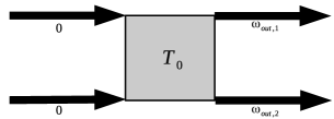
d)e)

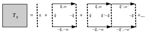
Figure 3: Feynman diagrams corresponding to a) first order, b) second order, c) third order contributions in $H_{dd}$. d) Schematic representation of the sum of all orders starting with the first. e) diagrammatic representation of the perturbative expansion of $T_{0}$. Here the thick arrows represent the Green’s functions $G_{ac},G_{ca}$, thin arrows stand for the polaritonic propagator $G_{cc}$ and, finally the dashed vertical lines represent the Fourier transform of the interaction potential $U$.

In Eq. (26) the term $\left(G_{c_{0}a}^{T}\left[0\right]\right)^{2}$ stands for the conversion of two incoming photons into symmetric Rydberg polaritons. Resulting from the resummation of diagrams of all perturbative orders in $H_{dd}$, the term $\frac{\left(-{\rm i}T_{0}\right)}{2\pi}$ represents the action of the Rydberg dipole-dipole-interaction-induced non-linearity on the two symmetric polaritons, provided they return to the symmetric subspace. Finally the term $G_{ac_{0}}^{T}\left[\omega_{out,1}\right]G_{ac_{0}}^{T}\left[\omega_{out,2}\right]$ represents the conversion of two symmetric polaritons back to the cavity mode photons. In conclusion, we note that $T_{0}$ can be derived analytically as we show in App. B.

VI $G^{\left(1\right)}$ correlation function

In this section we use Schwinger-Keldysh contour formalism in order to compute the correlation function $G_{out}^{\left(1\right)}\left(t,t^{\prime}\right)=\left\langle a_{out}^{\left(R\right)\dagger}\left(t\right)a_{out}^{\left(R\right)}\left(t^{\prime}\right)\right\rangle$ of the light transmitted through the cavity at fourth order in the feeding rate $\alpha$ as presented in (Grankin et al., 2016). By virtue of input-output relations this quantity is proportional to the correlation function of the intracavity fields, i.e. $G_{out}^{\left(1\right)}\left(t,t^{\prime}\right)=2\gamma_{c}^{\left(R\right)}\left\langle a^{\dagger}\left(t\right)a\left(t^{\prime}\right)\right\rangle$.

At second order in the feeding rate $\alpha$ Eq. (16) straightforwardly yields $\left\langle a^{\dagger}\left(t\right)a\left(t^{\prime}\right)\right\rangle^{\left(2\right)}=\left\langle a^{\dagger}\left(t\right)\right\rangle^{\left(1\right)}\left\langle a\left(t^{\prime}\right)\right\rangle^{\left(1\right)}$ which agrees with the factorization property shown in (Grankin et al., 2015). At fourth order in $\alpha$ this property does not hold any longer and Eq. (16) writes:

$$\left\langle a^{\dagger}\left(t\right)a\left(t^{\prime}\right)\right\rangle^{\left(4\right)}=\frac{\left(-\mathrm{i}\sqrt{2\pi}\alpha\right)^{4}}{4}\left\langle{\cal T}_{{\cal C}}\left\{e^{-\mathrm{i}\left(\int_{{\cal C}}H_{dd}\right)}A_{q}^{2}A_{q}^{\dagger 2}a_{-}^{\dagger}\left(t\right)a_{+}\left(t^{\prime}\right)\right\}\right\rangle$$ (29)

Note that we placed the operators $a_{-}^{\dagger}\left(t\right)$ and $a_{+}\left(t\right)$ on the $\mathcal{C}_{-}$ and $\mathcal{C}_{+}$ branches, respectively, in order to impose the normal ordering $a^{\dagger}\left(t\right)a\left(t^{\prime}\right)$ whatever $t$ and $t^{\prime}$ are. We now expand the correlation function Eq. (29) with respect to the dipole-dipole interactions, separating the forward and backward branches of the contour $\mathcal{C}$ as follows:

$$\left\langle a^{\dagger}\left(t\right)a\left(t^{\prime}\right)\right\rangle^{\left(4\right)}$$

$$= \frac{\left(-\mathrm{i}\sqrt{2\pi}\alpha\right)^{4}}{4}\sum_{p,q}\frac{\left(-{\rm i}\right)^{p+q}}{p!q!}\left\langle{\cal T}_{{\cal C}}\left\{\left(\int_{{\cal C}_{+}}dsH_{dd}\left(s\right)\right)^{p}\left(\int_{{\cal C}_{-}}dsH_{dd}\left(s\right)\right)^{q}A_{q}^{2}A_{q}^{\dagger 2}a_{-}^{\dagger}\left(t\right)a_{+}\left(t^{\prime}\right)\right\}\right\rangle$$

We first consider the partial resummation ${\cal E}\left(t,t^{\prime}\right)=\sum_{p=0,q>0}+\sum_{p>0,q=0}$ of Eq. (VI). Omitting the technical details of the derivation, which are provided in App. D, the Fourier transform of this contribution can be put under the form

$${\cal E}\left(\omega,\omega^{\prime}\right) = -2\pi\alpha^{4}\delta\left(\omega^{\prime}\right)\delta\left(\omega\right)G_{aa}^{*}\left[0\right]\left(G_{ac_{0}}^{T}\left[0\right]G_{ac_{0}}^{\tilde{T}}\left[0\right]\right)T_{0}\left(G_{c_{0}a}^{T}\left[0\right]\right)^{2}+{\rm c.c.}$$ (31)

where $T_{0}$ was defined in Eq. (27). Since $\left\langle a^{\dagger}\left(\omega\right)\right\rangle^{\left(3\right)}\varpropto\delta\left(\omega\right),$ and $\left\langle a\left(\omega^{\prime}\right)\right\rangle^{\left(1\right)}\varpropto\delta\left(\omega^{\prime}\right)$, we see that ${\cal E}\left(\omega,\omega^{\prime}\right)$ corresponds to the elastic part of the $G_{out}^{\left(1\right)}$ function at fourth order in feeding, i.e. $\left\langle a_{out}^{\left(R\right)\dagger}\left(\omega\right)a_{out}^{\left(R\right)}\left(\omega^{\prime}\right)\right\rangle_{el}\varpropto\delta\left(\omega\right)\delta\left(\omega^{\prime}\right)$, which is due to photons propagating through cavity without changing their frequency. Note that this fourth-order elastic contribution is actually a correction of the (necessarily elastic) second order spectrum.

VI.1 Inelastic contribution

As shown in App. D, the remaining contribution to Eq. (VI) takes the following form

$${\cal I}\left(\omega,\omega^{\prime}\right) = -\alpha^{4}\delta\left(\omega-\omega^{\prime}\right)\left|T_{0}\right|^{2}{\rm i}G_{c_{0}c_{0}}^{>}\left[-\omega\right]G_{c_{0}a}^{\tilde{T}}\left[\omega^{\prime}\right]G_{ac_{0}}^{T}\left[\omega\right]\left(G_{c_{0}a}^{T}\left[0\right]\right)^{2}\left(G_{ac_{0}}^{\tilde{T}}\left[0\right]\right)^{2}$$ (32)

and brings nonlinearity-induced inelastic features which were absent at lower orders.

The results derived above allows us to investigate the spectrum of the transmitted light

$$\mathcal{S}^{out}\left(\omega\right)\equiv\int d\omega^{\prime}G_{out}^{\left(1\right)}\left(\omega,\omega^{\prime}\right)$$

We are particularly interested in the inelastic part, i.e. ${\cal S}_{i}^{out}\equiv 2\gamma_{c}^{R}\int_{-\infty}^{\infty}d\nu\mathcal{I}\left(\omega,\nu\right)$ (see Eq. (32)), which is represented in Fig. 4 in resonant ($\Delta_{c}=\Delta_{e}=\Delta_{r}=0$) as well as detuned ($\Delta_{c}=-3\gamma_{e},\Delta_{e}=0,\Delta_{r}=0$) configurations. For both regimes we assume a cloud cooperativity $C=5$, and $\gamma_{c}^{R}=0.3\gamma_{e}\gg\gamma_{c}^{L}$ and $\gamma_{r}=0.15\gamma_{e}$ for the cavity and Rydberg decays respectively. All parameters are expressed in units of the intermediate state decay rate $\gamma_{e}=2\pi\times 3{\rm MHz}$.

As can be seen on Fig. 4 the spectrum exhibits several resonances which depend on the control field Rabi frequency. The resonance structure shown in Fig. 4 (a) (resonant case) resembles the level pattern of the Hamiltonian in the single excitation subspace

$$\left(\begin{array}[]{ccc}0&g\sqrt{N}&0\\ g\sqrt{N}&0&\frac{\Omega}{2}\\ 0&\frac{\Omega}{2}&0\end{array}\right)$$

In the detuned case, the structure shown on Fig. 4 (b) is more complicated; resonances can still be identified as the eigenvalues $\epsilon_{1},\epsilon_{2},\epsilon_{3}$ of the Hamiltonian

$$\left(\begin{array}[]{ccc}-\Delta_{c}&g\sqrt{N}&0\\ g\sqrt{N}&-\Delta_{e}&\frac{\Omega}{2}\\ 0&\frac{\Omega}{2}&-\Delta_{r}\end{array}\right)$$ (33)

but taken with positive and negative signs. This effect can be understood by inspecting the level structure of the considered system, shown in Fig. (a) 5 (Ourjoumtsev et al., 2011). The system can be excited by two photons of the probe laser frequency $\omega_{p}$. The strength of dipole-dipole interactions does not affect the $\omega$-dependence of the inelastic component at fourth order since $H_{dd}$ enters Eq. (32) only via the overall frequency-independent factor $\left|T_{0}\right|^{2}$. Doubly excited states decay via dissipative terms shown in the Heisenberg-Langevin equations Eqs. (17-19) to three symmetric polaritons of energies $\epsilon_{1},\epsilon_{2}$ and $\epsilon_{3}$ respectively. The resonance frequencies of the emitted photon pairs are therefore $\omega_{p}\pm\epsilon_{1}$, $\omega_{p}\pm\epsilon_{2}$ and $\omega_{p}\pm\epsilon_{3}$, respectively, or, in the frame rotating at the probe frequency $\omega_{p}$, $\pm\epsilon_{1}$, $\pm\epsilon_{2}$ and $\pm\epsilon_{3}$.

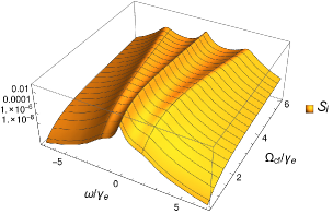
a)b)

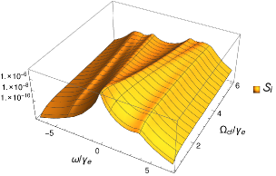
Figure 4: Inelastic component of the cavity transmission spectrum ${\cal S}_{i}\equiv 2\gamma_{c}^{R}\int d\nu\left\langle a^{\dagger}\left(\omega\right),a\left(\nu\right)\right\rangle$ in logarithmic scale as a function of $\Omega_{cf}$ and the frequency (in the frame rotating at $\omega_{p}$) for: a) the resonant case $\Delta_{c}=\Delta_{e}=\Delta_{r}=0$, b) the detuned case. The transverse curves give $\left(\pm\epsilon_{1},\pm\epsilon_{2},\pm\epsilon_{3}\right)$ as functions of $\Omega_{cf}$ (see main text).

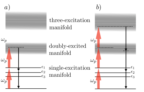
Figure 5: Schematic structure of the cavity-atom coupled system restricted to at most three excitations. The two-photon (a) and three-photon (b) cascades allow to understand the features observed in the cavity transmission spectrum (see Sec. VI) and the three-photon correlation function (Sec. VII)

VII Three-body effects

Until now, we dealt with quantities whose perturbative expansion involved at most two excitations. In this section we compute the three-photon wavefunction of the transmitted light $\left\langle a_{out}\left(\omega_{1}\right)a_{out}\left(\omega_{2}\right)a_{out}\left(\omega_{3}\right)\right\rangle^{\left(3\right)}$ whose calculation involves three-body terms. As in previous sections, we use input-output theory to relate $a_{out}$ to the intracavity field operator, and get:

$$\left\langle a_{out}\left(\omega_{1}\right)a_{out}\left(\omega_{2}\right)a_{out}\left(\omega_{3}\right)\right\rangle^{\left(3\right)}=\left(\sqrt{2\gamma_{c}}\right)^{3}\left\langle{\cal T}\left\{a\left(\omega_{1}\right)a\left(\omega_{2}\right)a\left(\omega_{3}\right)\right\}\right\rangle^{\left(3\right)}$$ (34)

Since we are focusing only on three-body effects, we discard one- and two-body terms by considering the quantity $\left\langle{\cal T}\left\{\delta a\left(\omega_{1}\right)\delta a\left(\omega_{2}\right)\delta a\left(\omega_{3}\right)\right\}\right\rangle^{\left(3\right)}$ where $\delta a\left(\omega\right)\equiv a\left(\omega\right)-\left\langle a\left(\omega\right)\right\rangle$:

$$\left\langle{\cal T}\left\{\delta a\left(\omega_{1}\right)\delta a\left(\omega_{2}\right)\delta a\left(\omega_{3}\right)\right\}\right\rangle^{\left(3\right)}$$ (35)

$$= \left\langle{\cal T}\left\{a\left(\omega_{1}\right)a\left(\omega_{2}\right)a\left(\omega_{3}\right)\right\}\right\rangle^{\left(3\right)}-\left\langle{\cal T}\left\{a\left(\omega_{1}\right)a\left(\omega_{2}\right)\right\}\right\rangle^{\left(2\right)}\left\langle a\left(\omega_{3}\right)\right\rangle^{\left(1\right)}-\left\langle{\cal T}\left\{a\left(\omega_{1}\right)a\left(\omega_{3}\right)\right\}\right\rangle^{\left(2\right)}\left\langle a\left(\omega_{2}\right)\right\rangle^{\left(1\right)}$$

$$-\left\langle{\cal T}\left\{a\left(\omega_{2}\right)a\left(\omega_{3}\right)\right\}\right\rangle^{\left(2\right)}\left\langle a\left(\omega_{1}\right)\right\rangle^{\left(1\right)}+2\left\langle a\left(\omega_{1}\right)\right\rangle^{\left(1\right)}\left\langle a\left(\omega_{2}\right)\right\rangle^{\left(1\right)}\left\langle a\left(\omega_{3}\right)\right\rangle^{\left(1\right)}$$

This term corresponds to the contribution of connected diagrams only in the full perturbative expansion of $\left\langle{\cal T}\left\{a\left(\omega_{1}\right)a\left(\omega_{2}\right)a\left(\omega_{3}\right)\right\}\right\rangle^{\left(3\right)}$. We now represent Eq. (35) in the contour-ordered form; noticing that only the forward part of the contour gives a non-vanishing contribution (by the same kind of arguments as in Sec. V) we get

$$\left\langle{\cal T}\left\{\delta a\left(\omega_{1}\right)\delta a\left(\omega_{2}\right)\delta a\left(\omega_{3}\right)\right\}\right\rangle^{\left(3\right)}=\frac{\left(-i\alpha\sqrt{2\pi}\right)^{3}}{3!}\left\langle{\cal T}\left\{a\left(\omega_{1}\right)a\left(\omega_{2}\right)a\left(\omega_{3}\right)e^{-i\int\left(H_{dd}\right)}\left(a^{\dagger}\left(0\right)\right)^{3}\right\}\right\rangle_{conn}$$ (36)

where the “conn” subscript stands for the summation over connected diagrams only. We can now expand the righthand side of this expression using Wick’s theorem. The resummation of diagrams is much simpler if we combine them in groups, following Faddeev’s original approach to three-body scattering (Faddeev, 1961).

VII.1 Partial resummation

In this subsection we perform the partial resummation of the perturbative expansion of Eq. (36). To this end, we first group diagrams so as to form elements of the two-body $T$-matrix expansion, as shown in Fig. 6 a) on an example. Such a combination of diagrams greatly facilitates the resummation: now the real interaction potential $\kappa_{ij}$ is merely replaced by $T$ matrices. The latter can effectively be considered as a new perturbation parameter, with respect to which the original correlation function Eq. (36) is expanded. The second-order terms in $T$ matrices of perturbation series are shown on Fig. 6 b) (the external lines are omitted analogously to App. B). It is natural to collect diagrams into three groups, depending on which lines are connected by the rightmost $T$-matrix. The corresponding partial resummations of the three sets, which can be called Faddeev components (Faddeev, 1961), are denoted by $\psi_{kl}\left(k,l=1,2,3\right)$ where $\left(k,l\right)$ are line indexes (see fig. 6 c).

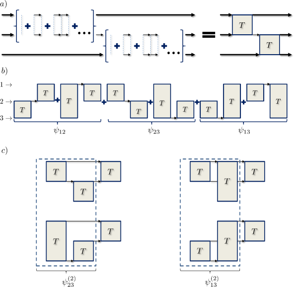
Figure 6: Diagrammatic expansion of the three-body correlation function: a) combination of ladder diagrams into two-body $T$-matrices, b) effective perturbative expansion with respect to $T$-matrices, c) expansion of $\psi_{12}^{\left(3\right)}$ to the third order with respect to $T$-matrices.

The first approximation we employ is to neglect hopping between atoms through the cavity, that is $T$ coincides with $\mathring{T}$ when $g$ is set to zero (see App. B). This constitutes a valid assumption in the regime when the number of blockaded atoms is much smaller than the total number of atoms. Under this approximation, it is convenient to work with real atomic positions instead of the reciprocal space. Expressed in the temporal Fourier space Eq. (36) therefore takes the form:

$$\left\langle{\cal T}\left\{\delta a\left(\omega_{1}\right)\delta a\left(\omega_{2}\right)\delta a\left(\omega_{3}\right)\right\}\right\rangle^{\left(3\right)}$$ (37)

$$= \sum_{r_{i},r_{j},r_{k}}\left(\alpha\sqrt{2\pi}\right)^{3}\delta\left(\sum\omega_{i}\right)G_{c_{i}a}\left[0\right]G_{c_{j}a}\left[0\right]G_{c_{k}a}\left[0\right]\left(\psi_{12}\left[\omega_{3}\right]+\psi_{23}\left[\omega_{2}\right]+\psi_{13}\left[\omega_{1}\right]\right)G_{ac_{i}}\left[\omega_{1}\right]G_{ac_{j}}\left[\omega_{2}\right]G_{ac_{k}}\left[\omega_{3}\right]$$

$$= \left(\alpha\sqrt{2\pi}G_{c_{0}a}\left[0\right]\right)^{3}\frac{\delta\left(\sum\omega_{i}\right)}{N^{3}}\sum_{r_{1},r_{2},r_{3}}\left(\psi_{12}\left[\omega_{3}\right]+\psi_{23}\left[\omega_{2}\right]+\psi_{13}\left[\omega_{1}\right]\right)G_{ac_{0}}\left[\omega_{1}\right]G_{ac_{0}}\left[\omega_{2}\right]G_{ac_{0}}\left[\omega_{3}\right]$$

where we used the following relation between Green’s functions $G_{ac_{0}}\left[\omega\right]\equiv\frac{1}{\sqrt{N}}\sum_{i}G_{ac_{i}}\left[\omega\right]=\sqrt{N}G_{ac_{i,k,j}}\left[\omega\right]$. According to these remarks, the second-order term in the expansion can be written in the following algebraic form:

$$\vec{\psi}^{\left(2\right)} \equiv\left(\begin{array}[]{c}\psi_{12}^{\left(2\right)}\left[\omega\right]\\ \psi_{23}^{\left(2\right)}\left[\omega\right]\\ \psi_{13}^{\left(2\right)}\left[\omega\right]\end{array}\right)=\left(\frac{-i}{2\pi}\right)^{2}\hat{B}\left[-\omega\right]iG_{c_{i}c_{i}}^{T}\left[-\omega\right]\vec{\psi}^{\left(1\right)}$$ (41)

where $$\vec{\psi}^{\left(1\right)}\equiv\left(\begin{array}[]{c}\mathring{T}_{12}\left[0\right]\\ \mathring{T}_{23}\left[0\right]\\ \mathring{T}_{13}\left[0\right]\end{array}\right)$$ (45)

$G_{c_{i}c_{i}}$ is the atomic Green’s function in real space under the no-hopping assumption (since all atoms are equivalent, these functions are equal), and we defined

$$\hat{B}\left[\omega\right]\equiv\left(\begin{array}[]{ccc}0&\mathring{T}_{12}\left[\omega\right]&\mathring{T}_{12}\left[\omega\right]\\ \mathring{T}_{23}\left[\omega\right]&0&\mathring{T}_{23}\left[\omega\right]\\ \mathring{T}_{13}\left[\omega\right]&\mathring{T}_{13}\left[\omega\right]&0\end{array}\right)$$

It is important to note, that $\vec{\psi}^{\left(1\right)}$ is not present in the expansion of Eq. (36), as it is a part of disconnected diagram series. The expansion of the $\psi_{12}$ component to the third order in $T$ is shown on Fig. 6 c) (the integration over each closed loop is implicit). From diagrammatics, we deduce:

$$\psi_{12}^{\left(3\right)} =\frac{-i}{2\pi}T_{12}\left[-\omega\right]\int d\xi iG_{c_{i}c_{i}}\left[-\xi-\omega\right]iG_{c_{i}c_{i}}\left[\xi\right]\psi_{23}^{\left(2\right)}\left[\xi\right]$$

$$+\frac{-i}{2\pi}T_{12}\left[-\omega\right]\int d\xi iG_{c_{i}c_{i}}\left[-\xi-\omega\right]iG_{c_{i}c_{i}}\left[\xi\right]\psi_{13}^{\left(2\right)}\left[\xi\right]$$

The structure of $\psi_{13}^{\left(3\right)}$ and $\psi_{23}^{\left(3\right)}$ is similar to those of $\psi_{12}^{\left(3\right)}$, and the full vector $\vec{\psi}^{\left(3\right)}$ can be put under the following matrix form:

$$\vec{\psi}^{\left(3\right)}\equiv\left(\begin{array}[]{c}\psi_{12}^{\left(3\right)}\left[\omega\right]\\ \psi_{23}^{\left(3\right)}\left[\omega\right]\\ \psi_{13}^{\left(3\right)}\left[\omega\right]\end{array}\right)=\frac{-i}{2\pi}\hat{B}\left[-\omega\right]\int d\xi iG_{c_{i}c_{i}}\left[-\xi-\omega\right]iG_{c_{i}c_{i}}\left[\xi\right]\vec{\psi}^{\left(2\right)}\left[\xi\right]$$ (46)

and, analogously, for the $\left(n+1\right)$-th order we can write:

$$\vec{\psi}^{\left(n+1\right)}=\frac{-i}{2\pi}\hat{B}\left[-\omega\right]\int d\xi iG_{c_{i}c_{i}}\left[-\xi-\omega\right]iG_{c_{i}c_{i}}\left[\xi\right]\vec{\psi}^{\left(n\right)}\left[\xi\right]$$ (47)

This iterative equation is equivalent to the following self-consistent equation (this can be checked directly by iterating the latter):

$$\vec{\psi}\left[\omega\right]=\frac{-i}{2\pi}\hat{B}\left[-\omega\right]\int d\xi iG_{c_{i}c_{i}}\left[-\xi-\omega\right]iG_{c_{i}c_{i}}\left[\xi\right]\vec{\psi}\left[\xi\right]+\vec{\psi}^{\left(2\right)}\left[\omega\right]$$ (48)

Let us first analyze the expression Eq. (47). The Green’s function $G_{c_{i}c_{i}}$ has two poles defined by $\omega_{p,1},\omega_{p,2}$ in the lower part of the complex plane (Abrikosov et al., 1975) (poles correspond to the two possible dressed states). Let us assume for now that the full solution of Eq. (48) $\vec{\psi}\left[\omega\right]$ has poles only in the upper part; we can then perform the integration in the right hand side of Eq. (48) and get via the residue theorem:

$$\vec{\psi}\left[\omega\right]=\hat{B}\left[-\omega\right]\eta_{1}\left[-\omega\right]\vec{\psi}\left[\omega_{p_{1}}\right]+\hat{B}\left[-\omega\right]\eta_{2}\left[-\omega\right]\vec{\psi}\left[\omega_{p_{2}}\right]+\vec{\psi}^{\left(2\right)}\left[\omega\right]$$ (49)

where $\eta_{j}\left[\omega\right]\equiv G_{c_{i}c_{i}}\left[\omega-\omega_{p_{j}}\right]\times\text{Res}_{\xi\rightarrow\omega_{p_{j}}}G_{c_{i}c_{i}}\left[\xi\right]$. In order to resolve the self-dependence in Eq. (49), we consider equations for $\vec{\psi}\left[\omega_{p_{1}}\right]$ and $\vec{\psi}\left[\omega_{p_{2}}\right]$ respectively:

$$\vec{\psi}\left[\omega_{p_{1}}\right]= \hat{B}\left[-\omega_{p_{1}}\right]\eta_{1}\left[-\omega_{p_{1}}\right]\vec{\psi}\left[\omega_{p_{1}}\right]+\hat{B}\left[-\omega_{p_{1}}\right]\eta_{2}\left[-\omega_{p_{1}}\right]\vec{\psi}\left[\omega_{p_{2}}\right]+\vec{\psi}^{\left(2\right)}\left[\omega_{p_{1}}\right]$$

$$\vec{\psi}\left[\omega_{p_{2}}\right]= \hat{B}\left[-\omega_{p_{2}}\right]\eta_{1}\left[-\omega_{p_{2}}\right]\vec{\psi}\left[\omega_{p_{1}}\right]+\hat{B}\left[-\omega_{p_{2}}\right]\eta_{2}\left[-\omega_{p_{2}}\right]\vec{\psi}\left[\omega_{p_{2}}\right]+\vec{\psi}^{\left(2\right)}\left[\omega_{p_{2}}\right]$$

which form a closed set of linear equations yielding:

$$\left(\begin{array}[]{c}\vec{\psi}\left[\omega_{p_{1}}\right]\\ \vec{\psi}\left[\omega_{p_{2}}\right]\end{array}\right)=\left(\begin{array}[]{cc}1-\hat{B}\left[-\omega_{p_{1}}\right]\eta_{1}\left[-\omega_{p_{1}}\right]&-\hat{B}\left[-\omega_{p_{1}}\right]\eta_{2}\left[-\omega_{p_{1}}\right]\\ -\hat{B}\left[-\omega_{p_{2}}\right]\eta_{1}\left[-\omega_{p_{2}}\right]&1-\hat{B}\left[-\omega_{p_{2}}\right]\eta_{2}\left[-\omega_{p_{2}}\right]\end{array}\right)^{-1}\left(\begin{array}[]{c}\vec{\psi}^{\left(2\right)}\left[\omega_{p_{1}}\right]\\ \vec{\psi}^{\left(2\right)}\left[\omega_{p_{2}}\right]\end{array}\right)$$ (50)

The analytical solution of Eq. (50) which can be obtained in e.g. Mathematica is cumbersome even in many limiting cases. It can, however, be dealt with numerically. Using Eq. (50) we can write the general solution of the self-consistent equation:

$$\vec{\psi}\left[\omega\right]=\left(\hat{B}\left[-\omega\right]\eta_{1}\left[-\omega\right],\hat{B}\left[-\omega\right]\eta_{2}\left[-\omega\right]\right)\times\left(\begin{array}[]{c}\vec{\psi}\left[\omega_{p_{1}}\right]\\ \vec{\psi}\left[\omega_{p_{2}}\right]\end{array}\right)+\vec{\psi}^{\left(2\right)}\left[\omega\right]$$ (51)

Finally, we check a posteriori our initial assumption, i.e. that Eq. (51) indeed has poles only in the upper part of the complex plane.

To conclude this subsection, we now briefly discuss how the reintroduction of hopping between atoms modifies the previous results at lowest order in $\nicefrac{{V_{b}}}{{V}}$. We first note that it is possible to derive the exact expression of the term $\vec{\psi}^{\left(2\right)}\left[\omega\right]$ standing on the right handside of Eq. (51) without assuming $g=0$, i.e. including hopping. Here we provide the final expression only, as the derivation is the same as above, but in the spatial Fourier space:

$$\sum_{r_{1},r_{2},r_{3}}\vec{\psi}_{g\neq 0}^{\left(2\right)}\left[\omega\right] =\left(\frac{-i}{2\pi}\right)^{2}iG_{c_{0}c_{0}}\left[-\omega\right]T_{0}\left[0\right]T_{0}\left[-\omega\right]\left(\begin{array}[]{c}1\\ 1\\ 1\end{array}\right)$$

$$\approx\left(\frac{-i}{2\pi}\right)^{2}iG_{c_{0}c_{0}}\left[-\omega\right]\mathring{T}_{0}\left[0\right]\mathring{T}_{0}\left[-\omega\right]\left(\begin{array}[]{c}1\\ 1\\ 1\end{array}\right)$$

where $T_{0}$ is given by Eq. (67), and in the last line we kept only the leading terms in $V_{b}/V$. It can also be shown that the contribution of hopping between atoms in the first term on the right handside of Eq. (51) is at least of the third order in $\nicefrac{{V_{b}}}{{V}}$, and can therefore be neglected in our approximation framework. Combining these remarks we can now numerically derive the three body correlation function. We note that this method can be extended to higher-order correlation functions.

VII.2 Numerical results and discussion

In this subsection we present the numerical results for the frequency distribution of correlation function Eq. (34).

A possible experimental scheme to measure the three-body (frequency-resolved) correlation function is suggested on Fig. 7. We assume that the light transmitted through the cavity is split into three paths by means of standard beam-splitters and sent to three different detectors, combined with narrow-band filters represented by cavities. In this case, it can be shown, that the total number of photons, jointly detected by all three detectors, is proportional to:

$$\int_{-\infty}^{\infty}dt_{1}dt_{2}dt_{3}\left\langle A^{\dagger}\left(t_{1}\right)B^{\dagger}\left(t_{2}\right)C^{\dagger}\left(t_{3}\right)C\left(t_{3}\right)B\left(t_{2}\right)A\left(t_{1}\right)\right\rangle\sim\left\langle a_{out}^{\dagger}\left(\omega_{1}\right)a_{out}^{\dagger}\left(\omega_{2}\right)a_{out}^{\dagger}\left(\omega_{3}\right)a_{out}\left(\omega_{3}\right)a_{out}\left(\omega_{2}\right)a_{out}\left(\omega_{1}\right)\right\rangle$$ (52)

where $A$, $B$ and $C$ are the respective annihilation operators of the input fields impinging on the three corresponding detectors (see Fig. 7). $\omega_{1},\omega_{2}$ and $\omega_{3}$ are the frequencies (in the frame, rotating at $\omega_{p}$) of filters (cavities). As can be seen from Eq. (52), it gives not only the connected three-body contribution to the correlation function but also the disconnected ones. However, if none of $\omega_{k}$’s in Eq. Eq. (52) is equal to zero, the result will contain only the desired part.

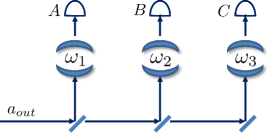
Figure 7: An experimental scheme for measurement of the three-photon correlation function $\left|\left\langle\delta a_{out}\left(\omega_{1}\right)\delta a_{out}\left(\omega_{2}\right)\delta a_{out}\left(\omega_{3}\right)\right\rangle^{\left(3\right)}\right|^{2}$.

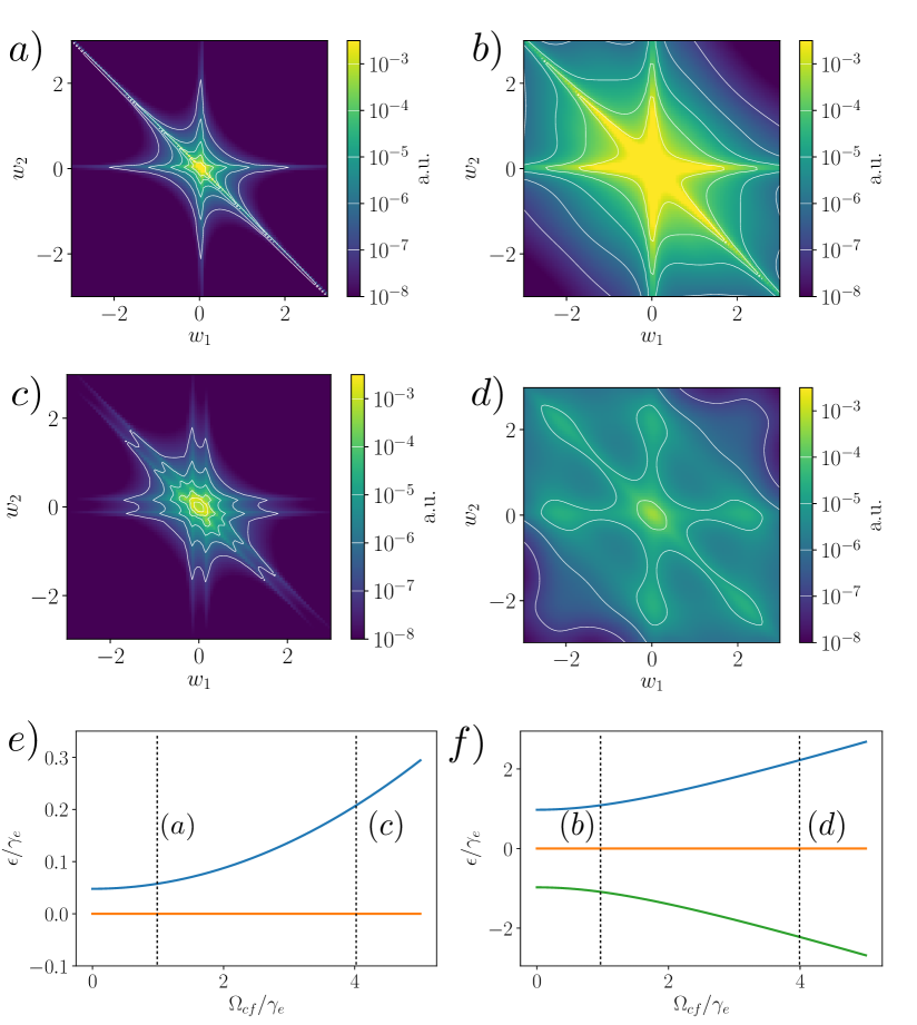
Figure 8: Three-photon correlation function $\left|\left\langle\delta a\left(\omega_{1}\right)\delta a\left(\omega_{2}\right)\delta a\left(-\omega_{1}-\omega_{2}\right)\right\rangle^{\left(3\right)}\right|$ as a function of $\omega_{1}$ and $\omega_{2}$: for the parameters a) $\Delta_{e}=-25\gamma_{e}$, $\Omega_{cf}=\gamma_{e}$, b) $\Delta_{e}=0$, $\Omega_{cf}=\gamma_{e}$, c) $\Delta_{e}=-25\gamma_{e}$, $,\Omega_{cf}=4\gamma_{e}$, d) $\Delta_{e}=0$, $\Omega_{cf}=4\gamma_{e}$. The polariton eigenstate energy for: e) detuned regime $\Delta_{e}=-25\gamma_{e}$, f) resonant case $\Delta_{e}=0$, $\epsilon_{1}$, $\epsilon_{2}$, $\epsilon_{3}$ energies are given by the blue, orange and green curves respectively. In the far detuned regime one of the polaritons eigenenergy is equal to $\epsilon_{3}$$\approx-25\gamma_{e}$ (not shown).

Fig. 8 displays numerical simulations of the third-order correlation function $\left\langle\delta a\left(\omega_{1}\right)\delta a\left(\omega_{2}\right)\delta a\left(-\omega_{1}-\omega_{2}\right)\right\rangle$ with respect to the frequencies $\left(\omega_{1},\omega_{2}\right)$ of two of the emitted photons – the third frequency is automatically set to $-\left(\omega_{1}+\omega_{2}\right)$ by conservation of energy in the frame rotating at $\omega_{p}$ – for different values of the control field $\Omega_{cf}$ and intermediate state detuning $\Delta_{e}$.

As for the second-order correlation function, we may interpret the structures observed on these plots by resorting to the three-photon cascade picture of Fig. 5 (b) and the polaritonic structure on Fig. 8 (e,f). When the coupled atom-cavity system absorbs three incoming probe photons, it is promoted to the three-excitation subspace, schematically represented as a quasi-continuum. When deexciting to its ground-state, the system reemits three photons of respective frequencies $\omega_{a}$ (upper transition), $\omega_{b}$ (intermediate transition) and $\omega_{c}$ (lower transition). Note that the triplet of frequencies $\left(\omega_{1},\omega_{2},-\omega_{1}-\omega_{2}\right)$ used in Fig. 8 alternatively play the role of all $6$ permutations of $\left(\omega_{a},\omega_{b},\omega_{c}\right)$. The frequency $\omega_{c}$ of the lower transition is constrained to three values given by the polaritonic eigenenergies $\epsilon_{1,2,3}$ represented on Fig. 8 (e,f). The frequency of the upper transition frequency which couples the three-excitation and two-excitation subspaces is not fixed but is rather constrained to belong to a window of width $\Delta\omega$ that we shall assume symmetric around origin (i.e. $\omega_{p}$ in the rotating frame). The intermediate transition frequency is related to the other two by the energy conservation $\omega_{a}+\omega_{b}+\omega_{c}=0$. Finally we get

$$-\frac{1}{2}\Delta\omega \leq\omega_{a}\leq\frac{1}{2}\Delta\omega$$

$$\omega_{b} =-\omega_{a}-\omega_{c}$$

$$\omega_{c} =\epsilon_{k=1,2,3}$$

In the far detuned case, diagonalizing the Hamiltonian of the atom-cavity-system in the single-excitation subspace yields the polaritonic structure of Fig. 8 (e) with two polaritons of close energies, the third being too far away to be represented on the plot. When these two energies are two close, i.e. when $\Omega_{cf}$ is too weak, the two cases $\omega_{c}=\epsilon_{1,2}$ cannot be distinguished : this case is represented on Fig. 8 (a) where three main lines can be identified, one vertical corresponding to $\omega_{1}=\omega_{c}=\epsilon_{1,2}$, one horizontal corresponding to $\omega_{2}=\omega_{c}=\epsilon_{1,2}$, one antidiagonal corresponding to $\omega_{3}=-\omega_{1}-\omega_{2}=\omega_{c}=\epsilon_{1,2}$. Note that the width $\Delta\omega$ limits the “visibility window” where the correlation function takes substantial values. By contrast, when the control field is larger, the two cases $\omega_{c}=\epsilon_{1,2}$ can be distinguished, which yields a double structure of six lines – two vertical, two horizontal, two antidiagonal – as can be seen on Fig. 8 (c).

In the resonant case, the symmetry of the polaritonic energy scheme of Fig. 8 (f) leads to a structure with $3\times 3=9$ lines – three vertical, three horizontal, three antidiagonal – which can be distinguished when $\Omega_{cf}$ is large enough, as in Fig. 8 (d), but merge when $\Omega_{cf}$ is too weak, as in Fig. 8 (b).

For sake of completeness, we underline that, although the above interpretation seems to agree well with our observations, there exists a slight discrepancy, for instance on Fig. 8 (c). According to the values of the polaritonic energies, we indeed expect to observe a vertical (horizontal) line centered on $\omega_{1}=0$ ($\omega_{2}=0$) : by contrast, the line we obtain is slightly shifted from the vertical (horizontal) axis. The reason for this effect could be an underlying structure within the two-excitation semi-continuum, that may be the object of further studies.

VIII Conclusion and perspectives

In this article, we theoretically investigated the nonlinear optical response of an atomic medium placed in a cavity and excited towards a Rydberg level in an EIT-configuration by a weak quantum probe and a strong control field. To this end, we made use of the so-called Schwinger-Keldysh contour technique, commonly employed in condensed matter non-equilibrium physics, which allows for the systematic perturbation expansion of expectation values of interest. As expected, our analytic calculations show that the strong dipole-dipole interactions between Rydberg polaritons lead to quantum nonlinearities, i.e. nonlinearities noticeable in the few-photon regime. In particular, here, we presented the detailed calculation of the $G^{(1)}$ correlation function up to the fourth order in the probe amplitude : this allowed us to derive the shape of the spectrum of the light transmitted through the cavity and reveal the existence of an inelastic component that we interpreted physically (Grankin et al., 2016). Using the Fadeev approach, we also investigated three-body effects by computing the three-photon correlation function of the transmitted light up to third order in the probe amplitude and suggested an experimental setup to measure this quantity. We moreover identified a strong correlation of the frequencies of the photons transmitted, reminiscent of the time correlation recently observed in MIT experiment in a free-space setup (Liang et al., 2017). The results presented here show the power and versatility of the Schwinger-Keldysh approach for the treatment strongly interacting atomic media for quantum optics. Though we used it to analyze a single-mode cavity setup, we think it should be profitable in the treatment of several-mode cavity systems for the investigation of quantum fluids of light and exotic states that can be designed in such experiments (Carusotto and Ciuti, 2013), as well as in free-space configurations where it could be an alternative to effective field theory.

Appendix A Pair correlation function $\left\langle{\cal T}\left(a\left(t\right)a\left(t^{\prime}\right)\right)\right\rangle$

In this appendix we provide the technical details of the derivation of Eq. (26) omitted in the main text. Keeping only the ${\cal C}_{+}$ part of the contour (for shortness we will omit $"+"$ indices in this section) Eq (25) writes:

$$\left\langle{\cal T}\left(a\left(t\right)a\left(t^{\prime}\right)\right)\right\rangle^{\left(2\right)}=\frac{\left(-\mathrm{i}\alpha\right)^{2}}{2!}\left\langle{\cal T}\left\{e^{-\mathrm{i}\frac{1}{2}\sum_{m,n}\kappa_{mn}\int dsc_{n}^{\dagger}c_{m}^{\dagger}c_{n}c_{m}}\left(\int dsa^{\dagger}\left(s\right)\right)^{2}a\left(t\right)a\left(t^{\prime}\right)\right\}\right\rangle$$ (53)

To evaluate this expression we now perform the perturbative expansion with respect to $H_{dd}$, to expressed in the spinwave basis derived in App. C:

$$H_{dd}=\frac{1}{2}\sum_{\vec{q},\vec{k}_{1},\vec{k}_{2}}U_{\vec{q}}c_{\vec{k}_{2}-\vec{q}}^{\dagger}c_{\vec{q}+\vec{k}_{1}}^{\dagger}c_{\vec{k}_{1}}c_{\vec{k}_{2}}$$

The zeroth order of the expansion of Eq. (53) in $H_{dd}$ yields

$$\left\langle{\cal T}\left(a\left(t\right)a\left(t^{\prime}\right)\right)\right\rangle^{\left(2,0\right)} = \frac{\left(-\mathrm{i}\alpha\right)^{2}}{2!}\left\langle{\cal T}\left\{\left(\int dsa^{\dagger}\left(s\right)\right)^{2}a\left(t\right)a\left(t^{\prime}\right)\right\}\right\rangle$$

$$= \left(-\mathrm{i}\alpha\right)^{2}\left(\int ds_{1}{\rm i}G_{aa}\left[t-s_{1}\right]\int ds_{2}{\rm i}G_{aa}\left[t^{\prime}-s_{2}\right]\right)$$

$$= \left(-\mathrm{i}\alpha\right)^{2}{\rm i}G_{aa}\left[\omega=0\right]{\rm i}G_{aa}\left[\omega=0\right]$$

$$\equiv \left\langle a\left(t\right)\right\rangle^{\left(1\right)}\left\langle a\left(t^{\prime}\right)\right\rangle^{\left(1\right)}$$

where the superscript ^(p,q) denotes the $p-th$ order in expansion in $\alpha$ and $q-th$ in $H_{dd}$. The factorization of $\left\langle{\cal T}\left(a\left(t\right)a\left(t^{\prime}\right)\right)\right\rangle^{\left(2,0\right)}$ constitutes an obvious consequence of the fact that, at zeroth order in $H_{dd}$, the system is completely linear.

The first order of the expansion in $H_{dd}$ writes:

$$\left\langle{\cal T}\left\{a\left(t\right)a\left(t^{\prime}\right)\right\}\right\rangle^{\left(2,1\right)} = \sum_{\vec{q},\vec{k}_{1},\vec{k}_{2}}\frac{-{\rm i}U_{\vec{q}}}{2}\frac{\left(-\mathrm{i}\alpha\right)^{2}}{2!}\left\langle{\cal T}\left\{\int dsc_{\vec{k}_{2}-\vec{q}}^{\dagger}c_{\vec{q}+\vec{k}_{1}}^{\dagger}c_{\vec{k}_{1}}c_{\vec{k}_{2}}\left(\int ds^{\prime}a^{\dagger}\left(s^{\prime}\right)\right)^{2}a\left(t\right)a\left(t^{\prime}\right)\right\}\right\rangle$$ (54)

According to Wick’s theorem, we now have to review all possible ways to pair creation and annihilation operators in (54). As shown in Subsection III.2, the matrix representation $\hat{G}^{T}\left[\omega\right]$ of the time-ordered Green’s function shows a block-diagonal structure in the basis $\left\{a_{0},b_{0},c_{0},\right.$$\left.\left\{b_{\vec{k}\neq 0},c_{\vec{k}\neq 0}\right\}\right\}$ which implies that the Green’s functions $G_{xy}^{T}\left(t-t^{\prime}\right)=-{\rm i}\left\langle{\cal T}\left\{x\left(t\right)y^{\dagger}\left(t^{\prime}\right)\right\}\right\rangle$ vanishes unless $x$ and $y$ simultaneously belong to the same set, either $\left\{a_{0},b_{0},c_{0}\right\}$ or $\left\{b_{\vec{k}\neq 0},c_{\vec{k}\neq 0}\right\}$. Therefore only contractions of operators all picked either in the set $\left\{a,b_{0},c_{0}\right\}$ or in the set $\left\{b_{\vec{k}\neq 0},c_{\vec{k}\neq 0}\right\}$ give non-vanishing contractions, whence

$$\left\langle{\cal T}\left\{a\left(t\right)a\left(t^{\prime}\right)\right\}\right\rangle^{\left(2,1\right)}=-{\rm i}\times U_{0}\left(-\mathrm{i}\alpha\right)^{2}\int ds_{1}ds_{2}ds_{3}G_{ac_{0}}\left[t,s_{1}\right]G_{ac_{0}}\left[t^{\prime},s_{1}\right]G_{c_{0}a}\left[s,s_{2}\right]G_{c_{0}a}\left[s,s_{3}\right]$$ (55)

Fourier transforming of Eq. (55) with respect to both $t$ and $t^{\prime}$ we get:

$$\left\langle{\cal T}\left\{a\left(\omega_{out,1}\right)a\left(\omega_{out,2}\right)\right\}\right\rangle^{\left(2,1\right)} = \frac{1}{2\pi}\int dtdt^{\prime}e^{{\rm i}\omega_{out,1}t}e^{{\rm i}\omega_{out,2}t^{\prime}}\left\langle{\cal T}\left\{a\left(t\right)a\left(t^{\prime}\right)\right\}\right\rangle^{\left(2,1\right)}$$ (56)

$$= \left(-\mathrm{i}\sqrt{2\pi}\alpha\right)^{2}\left(-{\rm i}\times\frac{U_{0}}{2\pi}\right)\delta\left(\omega_{out,1}+\omega_{out,2}\right)G_{ac_{0}}^{T}\left[\omega\right]G_{ac_{0}}^{T}\left[\omega^{\prime}\right]\left(G_{c_{0}a}^{T}\left[0\right]\right)^{2}$$

Note that the operator ${\cal T}$ appearing in $\left\langle{\cal T}\left\{a\left(\omega_{out,1}\right)a\left(\omega_{out,2}\right)\right\}\right\rangle^{\left(2,1\right)}$ does not refer to any hypothetical ordering in the frequency space; it is a mere notation meant to remind that this quantity was obtained by Fourier transforming the average of a time-ordered product in real time space.

Consider now the second order in expansion in $H_{dd}$:

$$\left\langle{\cal T}\left\{a\left(t\right)a\left(t^{\prime}\right)\right\}\right\rangle^{\left(2,2\right)} = \frac{\left(-\mathrm{i}\sqrt{2\pi}\alpha\right)^{2}}{2^{3}}\sum_{\vec{q},\vec{k}_{1},\vec{k}_{2},\vec{k}_{1}^{\prime},\vec{k}_{2}^{\prime}\vec{q}^{\prime},}\left(\frac{-{\rm i}U_{-\vec{q}}}{2\pi}\right)\left(\frac{-{\rm i}U_{\vec{q}^{\prime}}}{2\pi}\right)$$

$$\times \left\langle{\cal T}\left\{\begin{array}[]{c}a\left(t\right)a\left(t^{\prime}\right)\int ds_{1}c_{\vec{k}_{2}-\vec{q}}^{\dagger}\left(s\right)c_{\vec{q}+\vec{k}_{1}}^{\dagger}\left(s\right)c_{\vec{k}_{1}}\left(s\right)c_{\vec{k}_{2}}\left(s\right)\\ \times\int ds_{2}c_{\vec{k}_{2}^{\prime}-\vec{q}^{\prime}}^{\dagger}\left(s_{2}\right)c_{\vec{q}^{\prime}+\vec{k}_{1}^{\prime}}^{\dagger}\left(s_{2}\right)c_{\vec{k}_{1}^{\prime}}\left(s_{2}\right)c_{\vec{k}_{2}^{\prime}}\left(s_{2}\right)\left(\frac{1}{\sqrt{2\pi}}\int dsa^{\dagger}\left(s\right)\right)^{2}\end{array}\right\}\right\rangle$$

Using the same remark as made above for the first order and using that, the contribution of “disconnected diagrams” (i.e. the contraction arrangement in which the $\left(4p\right)$ atomic operators of $\left(-{\rm i}\int_{{\cal C}_{+}}H_{dd}\right)^{p}$are paired with each other and therefore are disconnected from the other terms) vanishes(Abrikosov et al., 1975), we get in the temporal Fourier space:

$$\left\langle{\cal T}\left\{a\left(\omega_{out,1}\right)a\left(\omega_{out,2}\right)\right\}\right\rangle^{\left(2,2\right)}$$ (58)

$$= \left(-\mathrm{i}\sqrt{2\pi}\alpha G_{c_{0}a}^{T}\left[0\right]\right)^{2}\delta\left(\omega_{out,1}+\omega_{out,2}\right)G_{ac_{0}}^{T}\left[\omega_{out,1}\right]G_{ac_{0}}^{T}\left[\omega_{out,2}\right]\sum_{\vec{q}}\left(\frac{-{\rm i}U_{-\vec{q}}}{2\pi}\right)\left(\frac{{\rm i}U_{\vec{q}}}{2\pi}\right)\left(\int d\omega G_{c_{\vec{q}},c_{\vec{q}}}^{T}\left[\omega\right]G_{c_{-\vec{q}},c_{-\vec{q}}}^{T}\left[-\omega\right]\right)$$

The further expansion in $H_{dd}$ reveals a self-similar form which can be conveniently expressed using a diagrammatic representation. According to the latter, the Green’s functions of different kinds are represented by different arrows (see Fig. 3), while the interaction potential is represented by a vertical dashed line; it is moreover implicit that, for each loop in a diagram, integration (summation) should be performed over internal variables (indices) and that the overall expression obtained should be multiplied by the factor $\left(-\mathrm{i}\sqrt{2\pi}\alpha\right)^{2}\delta\left(\omega_{out,1}+\omega_{out,2}\right)\left(\frac{-{\rm i}}{2\pi}\right)^{p}$ where $p$ is the order in $H_{dd}$, i.e. the number of dashed vertical lines. Note that we do not distinguish $G_{ac_{0}}\left[\omega\right]$ and $G_{c_{0}a}\left[\omega\right]$ graphically since their expressions coincide (see Eq. (21)).

It is easy to see that diagrams (a), (b), (c) in Fig. 3, which represent $\left\langle{\cal T}\left\{a\left(\omega_{out,1}\right)a\left(\omega_{out,2}\right)\right\}\right\rangle^{\left(2,p\right)}$ for $p=1,2,3$, have four thick lines in common. These thick lines represent the conversion of a photon from the cavity mode to the symmetric Rydberg polariton and back. As there is no integration over the arguments of the corresponding Green’s function we can factorize them (Fig. 3 d). The remaining part of the correlation function is denoted by $T_{0}$; its perturbative expansion is diagrammatically represented in Fig. 3 (e).

From Fig. 3 (d) we finally get Eq. (26) of the main text.

Appendix B Calculation of the 2 body T-matrix

a)

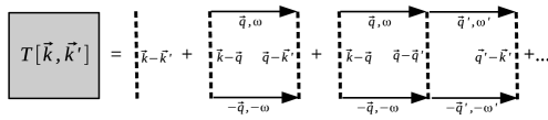
b)

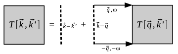
Figure 9: Diagrammatic representation of $T\left[\vec{k},\vec{k}^{\prime}\right]$ in a) perturbative form, b) self-consistent form.

As discussed in App. A, $T_{0}$ describes the combination of all possible interaction-induced scattering processes in which two incoming Rydberg polaritons are converted back to the same symmetric spinwaves. This quantity actually appears as a specific value of a more general function which describes the scattering of two arbitrary (i.e. not necessarily symmetric) Rydberg polaritons only constrained by the conservation of the sum of the wavevectors. This latter function is denoted by $T\left[\vec{k},\vec{k}^{\prime},\vec{P}\right]$ where $k\equiv\frac{\vec{k}_{in,1}-\vec{k}_{in,2}}{2}$ and $\vec{k}^{\prime}\equiv\frac{\vec{k}_{out,1}-\vec{k}_{out,2}}{2}$ are the differences of the incoming/outgoing spinwave’s wavevectors $\vec{k}_{\left(in/out\right),1},\vec{k}_{\left(in/out\right),2}$ respectively, and $\vec{P}=\vec{k}_{in,1}+\vec{k}_{in,2}$ is their (necessarily conserved) sum. The symmetry of the coupling between the cavity mode and the atoms restricts the possible values of the wavevectors: we are therefore entitled to consider only the $\vec{P}=0$ component, and denote $T\left[\vec{k},\vec{k}^{\prime},\vec{P}=0\right]\equiv T\left[\vec{k},\vec{k}^{\prime}\right]$.

The diagrammatic representation of $T\left[\vec{k},\vec{k}^{\prime}\right]$ ( given in Fig.9 a) is similar to the one obtained for $T_{0}$. From the diagrammatic structure it is easy to infer its self-consistent definition shown in Fig.9 b). The corresponding equation is readily obtained using the correspondence rules specified in Fig. 3:

$$T\left[\vec{k},\vec{k}^{\prime}\right] = U_{\vec{k}-\vec{k}^{\prime}}+{\rm i}\sum_{\vec{q}}U_{\vec{k}-\vec{q}}S_{\vec{q}}T\left[\vec{q},\vec{k}^{\prime}\right]$$ (59)

where $S_{\vec{q}}$ is defined in Eq. 28. As shown in Sec. III.2, all Green’s functions $G_{c_{\vec{q}}c_{\vec{q}}}$ have the same expression for $\vec{q}\neq 0$; we therefore define $S_{\vec{q}\neq 0}\equiv S$ and Eq. 59 writes:

$$T\left[\vec{k},\vec{k}^{\prime}\right] = U_{\vec{k}-\vec{k}^{\prime}}+{\rm i}\sum_{\vec{q}}U_{\vec{k}-\vec{q}}ST\left[\vec{q},\vec{k^{\prime}}\right]+{\rm i}U_{\vec{k}}\left(S_{0}-S\right)T\left[0,\vec{k}^{\prime}\right]$$ (60)

It is convenient to represent this equation in the matrix form

$$\widehat{T}=\widehat{{\cal U}}+{\rm i}S\,\widehat{{\cal U}}\cdotp\widehat{T}+{\rm i}\left(S_{0}-S\right)\widehat{{\cal U}}\cdotp{\cal P}^{\left(0\right)}\cdotp\widehat{T}$$

where $\widehat{T}_{\vec{k},\vec{k}^{\prime}}\equiv T\left[\vec{k},\vec{k}^{\prime}\right]$, $\widehat{{\cal U}}_{\vec{k},\vec{k}^{\prime}}\equiv U_{\vec{k}-\vec{k}^{\prime}}$ and ${\cal P}_{\vec{k},\vec{k}^{\prime}}^{\left(0\right)}\equiv\delta\left(\vec{k}\right)\delta\left(\vec{k}^{\prime}\right)$ is the projector onto the zeroth spinwave. Finally,

$$\widehat{T}=\left(1-{\rm i}S\,\widehat{{\cal U}}\right)^{-1}\cdotp\widehat{{\cal U}}\cdotp\left(\mathbb{I}+{\rm i}\left(S_{0}-S\right)\,{\cal P}^{\left(0\right)}\cdotp\widehat{T}\right)$$ (61)

There is no obvious straightforward way to extract $\widehat{T}$ from Eq. (61) in the general case. We may however relate $\widehat{T}$ to its value in the hypothetical configuration when the atoms decouple from the cavity, i.e. when atom-cavity coupling coefficient vanishes i.e. $g=0$.

In the latter condition from Eq. (21) we infer that $G_{c_{\vec{q}}c_{\vec{q}}}^{T}\left[\omega\right]=G_{c_{0}c_{0}}^{T}\left[\omega\right]$ whence $S=S_{0}$. In this specific configuration, the matrix $\widehat{T}$, that we shall denote $\widehat{\mathring{T}}$, to distinguish it from the general case, obeys $\widehat{\mathring{T}}=\widehat{{\cal U}}+{\rm i}S\,\widehat{{\cal U}}\cdotp\widehat{\mathring{T}}$ , whence $\widehat{\mathring{T}}=\left(1-{\rm i}S\widehat{{\cal U}}\right)^{-1}\cdotp\widehat{{\cal U}}$. Eq. (61) yields:

$$\widehat{T}=\widehat{\mathring{T}}\cdotp\left(\mathbb{I}+{\rm i}\left(S_{0}-S\right)\,{\cal P}^{0}\cdotp\widehat{T}\right)$$ (62)

Multiplying both sides of Eq. (62) by ${\cal P}^{\left(0\right)}\cdotp$ and solving for ${\cal P}^{\left(0\right)}\cdotp\widehat{T}$ we get:

$${\cal P}^{\left(0\right)}\cdotp\widehat{T}=\frac{{\cal P}^{\left(0\right)}\cdotp\widehat{\mathring{T}}}{1-{\rm i}\left(S_{0}-S\right)\,\mathring{T}_{0}}$$

where ${\cal P}^{\left(0\right)}\cdotp\widehat{\mathring{T}}\cdotp{\cal P}^{\left(0\right)}\equiv\mathring{T}_{0}{\cal P}^{\left(0\right)}$. Substituting this expression into Eq. (62) we finally get the expression for the $T$ matrix:

$$\widehat{T}=\widehat{\mathring{T}}+{\rm i}\left(S_{0}-S\right)\,\frac{\widehat{\mathring{T}}\cdotp{\cal P}^{\left(0\right)}\cdotp\widehat{\mathring{T}}}{1-{\rm i}\left(S_{0}-S\right)\,\mathring{T}_{0}}$$ (63)

Since we are interested in determining $T_{0}=T\left[0,0\right]={\rm Tr}\left\{{\cal P}^{\left(0\right)}\cdotp\widehat{T}\cdotp{\cal P}^{\left(0\right)}\right\}$ we multiply Eq. (63) by ${\cal P}^{\left(0\right)}$ on the left and right sides and get:

$$T_{0}=\frac{\mathring{T_{0}}}{1-{\rm i}\mathring{T_{0}}\left(S_{0}-S\right)}$$ (64)

The advantage of this relation is that $\mathring{T_{0}}$ can be evaluated exactly. From Eq. (59) with $S=S_{0}$ we get:

$$\mathring{T}\left[\vec{k},\vec{k}^{\prime}\right] = U_{\vec{k}-\vec{k}^{\prime}}+{\rm i}S\sum_{\vec{q}}U_{\vec{k}-\vec{q}}\mathring{T}\left[\vec{q},\vec{k}^{\prime}\right]$$

This equation can be easily solved in the real space using $U_{\vec{K}}=\frac{1}{N}\sum_{m}^{N}\kappa\left(\vec{r}_{m}\right)e^{i\vec{K}\vec{r_{m}}}$ (see App. C) :

$$\mathring{T}\left[\vec{r},\vec{r}^{\prime}\right] \equiv \frac{1}{N}\sum_{\vec{k},\vec{k}^{\prime}}e^{-{\rm i}\vec{k}\vec{r}}e^{{\rm i}\vec{k}^{\prime}\vec{r}^{\prime}}\mathring{T}\left[\vec{k},\vec{k}^{\prime}\right]=\kappa\left(\vec{r}\right)\delta_{\vec{r},\vec{r}^{\prime}}+{\rm i}S\kappa\left(\vec{r}\right)\mathring{T}\left[\vec{r},\vec{r}^{\prime}\right]$$

where $\vec{r}$ and $\vec{r}^{\prime}$ denote the real space conjugate coordinates to $\vec{k}$ and $\vec{k}^{\prime}$, respectively, and $\kappa\left(R\right)=\frac{C_{6}}{R^{6}}$. Finally we get:

$$\mathring{T}\left[\vec{r},\vec{r}^{\prime}\right] = \frac{\kappa\left(\vec{r}\right)}{1-{\rm i}S\kappa\left(\vec{r}\right)}\delta_{\vec{r},\vec{r}^{\prime}}$$ (65)

Using this expression and transforming back to the spinwave space we get $\mathring{T}\left[0,0\right]=\frac{1}{N}\sum_{i}\frac{\kappa\left(\vec{r}_{i}\right)}{1-{\rm i}S\kappa\left(\vec{r}_{i}\right)}$. We may finally approximate $\mathring{T}_{0}$ by an integral assuming the size of the sample to be sufficiently big, and in the case $C_{6}<0$ we get:

$$\mathring{T}_{0} \approx \frac{1}{V}\int_{V}d^{3}R\frac{\kappa\left(R\right)}{1-{\rm i}SV\left(R\right)}\approx-\frac{2\pi^{2}}{3V}\sqrt{\frac{-{\rm i}\left|C_{6}\right|}{S}}$$ (66)

Note, that the Eq. (65) characterizes the atomic density-density correlation function: it is maximal if two atoms are blocking each other and zero if atoms are not interacting. Consequently, $\mathring{T}_{0}$ is proportional to the ratio of the volume of a blockade sphere $\left(V_{b}\right)$ to the total volume of the sample. The expression for $V_{b}$ is consistent with the previously obtained results (Stanojevic et al., 2013; Grankin et al., 2015).

Now combining Eqs. (64, 66) we finally have:

$$T_{0}=\frac{-\frac{2\pi^{2}}{3V}\sqrt{\frac{-{\rm i}\left|C_{6}\right|}{S}}}{1+{\rm i}\left(S_{0}-S\right)\frac{2\pi^{2}}{3V}\sqrt{\frac{-{\rm i}\left|C_{6}\right|}{S}}}$$ (67)

Substituting this expression into Eq. (26) we can get an expression for the non-linear part of the pair correlation function in Fourier space. We recover exactly the same expression as in (Grankin et al., 2015), though in a much more concise form.

Appendix C Spinwave basis

In this appendix, we introduce the collective atomic modes known as “spinwaves”, which play a crucial role due to the symmetries of the problem and lead to a simpler expression of the full Hamiltonian.

First, we assume that atoms occupy the vertices of a 3D square lattice of step $\delta$. In all calculations we will eventually set the limit $\delta\rightarrow 0$ and therefore consider a continuous medium but we will keep the discrete sums in all expressions for the sake of convenience. The discrete Fourier transform allows us to relate the direct space bosonic operators $b_{j}$ and $c_{j}$ to the reciprocal space collective (so-called) spinwave operators $b_{\vec{k}},c_{\vec{k}}$:

$$c_{\vec{k}} = \frac{1}{\sqrt{N}}\sum_{j}e^{i\vec{k}\vec{r_{j}}}c_{j}\leftrightarrow c_{j}=\frac{1}{\sqrt{N}}\sum_{\vec{k}}e^{-i\vec{k}\vec{r_{j}}}c_{\vec{k}}$$ (68)

$$b_{\vec{k}} = \frac{1}{\sqrt{N}}\sum_{j}e^{i\vec{k}\vec{r_{j}}}b_{j}\leftrightarrow b_{j}=\frac{1}{\sqrt{N}}\sum_{\vec{k}}e^{-i\vec{k}\vec{r_{j}}}b_{\vec{k}}$$ (69)

where $\vec{r}_{i}$ is the position of the $i$-th atom and $k_{x,y,z}=-\nicefrac{{\pi}}{{\delta}},-\nicefrac{{\pi}}{{\delta}}+\frac{2\pi}{L_{x,y,z}}.\ldots,\nicefrac{{\pi}}{{\delta}}$ are the components of the $\vec{k}$ vector, where $L_{x,y,z}$ is the lattice dimension in the $\left\{x,y,z\right\}$ direction . One readily shows

$$\left[c_{\vec{k}},c_{\vec{k}^{\prime}}^{\dagger}\right] = \frac{1}{N}\sum_{m,n}e^{i\vec{k}\vec{r_{m}}}e^{-i\vec{k}^{\prime}\vec{r_{n}}}\left[c_{m},c_{n}^{\dagger}\right]=\frac{1}{N}\sum_{m}e^{i\vec{k}\vec{r}_{m}}e^{-i\vec{k}^{\prime}\vec{r}_{m}}=\delta_{\vec{k},\vec{k}^{\prime}}$$

and similarly $\left[b_{\vec{k}},b_{\vec{k}^{\prime}}^{\dagger}\right]=\delta_{\vec{k},\vec{k}^{\prime}}$. We now rewrite the dipole-dipole Hamiltonian in terms of the spinwaves operators defined above

$$H_{dd} =\frac{1}{2N^{2}}\sum_{m,n}^{N}\kappa_{mn}\sum_{\vec{k}^{\prime\prime\prime},\vec{k}^{\prime\prime},\vec{k}^{\prime},\vec{k}}e^{i\left(\vec{k}^{\prime\prime\prime}-\vec{k}\right)\vec{r_{n}}}e^{i\left(\vec{k}^{\prime\prime}-\vec{k}^{\prime}\right)\vec{r_{m}}}c_{\vec{k}^{\prime\prime\prime}}c_{\vec{k}^{\prime\prime}}c_{\vec{k}^{\prime}}c_{\vec{k}}$$ (70)

Imposing periodic boundary conditions on $\kappa_{mn}$, we obtain

$$\frac{1}{N^{2}}\sum_{m,n}^{N}\kappa_{mn}e^{i\left(\vec{k}^{\prime\prime\prime}-\vec{k}\right)\vec{r_{n}}}e^{i\left(\vec{k}^{\prime\prime}-\vec{k}^{\prime}\right)\vec{r_{m}}} = U_{\vec{k}^{\prime\prime}-\vec{k}^{\prime}}\frac{1}{N}\sum_{n}^{N}e^{i\left(\vec{k}^{\prime\prime}-\vec{k}^{\prime}+\vec{k}^{\prime\prime\prime}-\vec{k}\right)\vec{r_{n}}}$$ (71)

$$= U_{\vec{k}^{\prime\prime}-\vec{k}^{\prime}}\delta\left(\vec{k}^{\prime\prime}-\vec{k}^{\prime}+\vec{k}^{\prime\prime\prime}-\vec{k}\right)$$

where we defined the Fourier transform of the interaction matrix $\kappa_{mn}$ as $\frac{1}{N}\sum_{m}^{N}\kappa_{nm}e^{i\vec{K}\vec{r_{m}}}\equiv U_{\vec{K}}e^{i\vec{K}\vec{r_{n}}}$. Substituting Eq. (71) into Eq. (70) we get

$$H_{dd} =\sum_{\vec{k}^{\prime},\vec{k},\vec{q}}U_{\vec{q}}c_{\vec{k}^{\prime}-\vec{q}}c_{\vec{k}^{\prime}+\vec{q}}c_{\vec{k}^{\prime}}c_{\vec{k}}$$ (72)

where summations can be taken within any period of the lattice and will be omitted for the sake of conciseness.

Appendix D Transmission Spectrum technical details

In this appendix we provide technical details of the derivation of the elastic and inelastic contributions of the transmission spectrum, omitted in Sec. V.

D.1 Elastic contribution

We define the elastic contribtion to the spectrum as the partial resummation ${\cal E}\left(t,t^{\prime}\right)=\sum_{p=0,q>0}+\sum_{p>0,q=0}$ of Eq. (VI). We first consider the partial sum of Eq. (VI) including the terms $p\neq 0,q=0$, we get:

$$\frac{\left(-\mathrm{i}\sqrt{2\pi}\alpha\right)^{4}}{4}\sum_{p}\frac{\left(-{\rm i}\right)^{p}}{p!}\left\langle{\cal T}_{{\cal C}}\left\{\left(\frac{1}{2}\sum_{m,n}\kappa_{mn}\int_{\mathcal{C}_{+}}dsc_{n}^{\dagger}c_{m}^{\dagger}c_{n}c_{m}\right)^{p}A_{q}^{2}A_{q}^{\dagger 2}a_{-}^{\dagger}\left(t\right)a_{+}\left(t^{\prime}\right)\right\}\right\rangle$$ (73)

Using the results of Subsec. IV we see that the operator $a_{-}^{\dagger}\left(t\right)$ does not have other candidates for contraction than $A_{q}$. Since $\left\langle a^{\dagger}\left(t\right)\right\rangle^{\left(1\right)}=\left(-\sqrt{2\pi}{\rm i}\alpha\right)\left\langle{\cal T}_{{\cal C}}\left\{a_{-}^{\dagger}\left(t\right)A_{q}\right\}\right\rangle$ (see Sec. IV),

$$\frac{\left(-\mathrm{i}\sqrt{2\pi}\alpha\right)^{3}}{2}\sum_{p}\frac{\left(-{\rm i}\right)^{p}}{p!}\left\langle{\cal T}_{{\cal C}}\left\{\left(\frac{1}{2}\sum_{m,n}\kappa_{mn}\int_{\mathcal{C}_{+}}dsc_{n}^{\dagger}c_{m}^{\dagger}c_{n}c_{m}\right)^{p}A_{q}A_{q}^{\dagger 2}a_{+}\left(t^{\prime}\right)\right\}\right\rangle\times\left\langle a^{\dagger}\left(t\right)\right\rangle^{\left(1\right)}$$ (74)

From the general formula Eq. (16) we have:

$$\left\langle a\left(t\right)\right\rangle^{\left(3\right)} \equiv \frac{\left(-\mathrm{i}\sqrt{2\pi}\alpha\right)^{3}}{2!}\sum_{p,q}\frac{\left(-{\rm i}\right)^{p+q}}{p!q!}\left\langle\begin{array}[]{c}{\cal T}_{{\cal C}}\left\{\left(\frac{1}{2}\sum_{m,n}\kappa_{mn}\int_{{\cal C}_{+}}c_{n}^{\dagger}c_{m}^{\dagger}c_{n}c_{m}\right)^{p}\right.\\ \times\left.\left(\frac{1}{2}\sum_{m,n}\kappa_{mn}\int_{{\cal C}_{-}}c_{n}^{\dagger}c_{m}^{\dagger}c_{n}c_{m}\right)^{q}A_{q}A_{q}^{\dagger 2}a_{+}\left(t\right)\right\}\end{array}\right\rangle$$

In the expression above one of the operators $c_{n}^{\dagger},c_{m}^{\dagger}$ belonging the ${\cal C}_{-}$ branch does not have any partner for contraction. Therefore only the $q=0$ term will contribute to the sum and

$$\left\langle a\left(t\right)\right\rangle^{\left(3\right)}=\frac{\left(-\mathrm{i}\sqrt{2\pi}\alpha\right)^{3}}{2!}\left\langle{\cal T}_{{\cal C}}\left\{e^{-\mathrm{i}\frac{1}{2}\sum_{m,n}\kappa_{mn}\int_{{\cal C}_{+}}dsc_{n}^{\dagger}c_{m}^{\dagger}c_{n}c_{m}}A_{q}A_{q}^{\dagger 2}a_{+}\left(t\right)\right\}\right\rangle$$ (76)

Eq. (74) therefore writes $\left\langle a^{\dagger}\left(t\right)\right\rangle^{\left(1\right)}\left\langle a\left(t^{\prime}\right)\right\rangle^{\left(3\right)}$.

Analogously, the partial sum of the terms $\left(p=0,q\neq 0\right)$ yields $\left\langle a^{\dagger}\left(t\right)\right\rangle^{\left(3\right)}\left\langle a\left(t^{\prime}\right)\right\rangle^{\left(1\right)}$. Finally we get

$${\cal E}=\left\langle a^{\dagger}\left(t\right)\right\rangle^{\left(3\right)}\left\langle a\left(t^{\prime}\right)\right\rangle^{\left(1\right)}+\left\langle a^{\dagger}\left(t\right)\right\rangle^{\left(1\right)}\left\langle a\left(t^{\prime}\right)\right\rangle^{\left(3\right)}$$ (77)

We shall now determine the expression for $\left\langle a\left(t\right)\right\rangle^{\left(3\right)}$. Let us perform an expansion of Eq. (76) with respect to $H_{dd}$. Due to the symmetry properties of the system, it is more convenient to work in the spatial Fourier space. We therefore get:

$$\left\langle a\left(t\right)\right\rangle^{\left(3\right)} = \frac{\left(-\mathrm{i}\sqrt{2\pi}\alpha\right)^{3}}{2!}\sum_{p}\frac{1}{p!}\left\langle{\cal T}_{{\cal C}}\left\{\left(-\frac{{\rm i}}{2}\sum_{\vec{q},\vec{k}_{1},\vec{k}_{2}}U_{\vec{q}}\int_{{\cal C}_{+}}c_{\vec{k}_{2}-\vec{q}}^{\dagger}c_{\vec{q}+\vec{k}_{1}}^{\dagger}c_{\vec{k}_{1}}c_{\vec{k}_{2}}\right)^{p}A_{q}A_{q}^{\dagger 2}a_{+}\left(t\right)\right\}\right\rangle$$

As expected, the zeroth order $\left(p=0\right)$ of this expansion is zero since it necessarily involves the vanishing contraction of two “quantum” operators $A_{q}$ and $A_{q}^{\dagger}$ (see Sec. III.2). Apart from the external lines, the terms in the expansion with $p>1$ form the same ladder series as derived in App. B. The difference in the external lines is given by the replacement of one of $a_{+}$ operators by $A_{q}$: the corresponding contraction is given by:

$$\left\langle{\cal T}_{{\cal C}}\left\{A_{q}c_{+,\vec{k}}^{\dagger}\left(t\right)\right\}\right\rangle = \frac{1}{\sqrt{2\pi}}\int ds\left\langle{\cal T}_{{\cal C}}\left\{\left(a_{+}\left(s\right)-a_{-}\left(s\right)\right)c_{+,\vec{k}}^{\dagger}\left(t\right)\right\}\right\rangle=\frac{1}{\sqrt{2\pi}}\int ds\left\{-iG_{ac_{0}}^{\tilde{T}}\left[s,t\right]\right\}\delta_{\vec{k},0}$$

Combining these remarks, we get in the frequency space:

$$\left\langle a\left(\omega\right)\right\rangle^{\left(3\right)}=\left(-\mathrm{i}\sqrt{2\pi}\alpha\right)^{3}\delta\left(\omega\right)\left(-{\rm i}G_{ac_{0}}^{T}\left[0\right]{\rm i}G_{ac_{0}}^{\tilde{T}}\left[0\right]\right)\left(\frac{-{\rm i}T_{0}}{2\pi}\right)\left({\rm i}G_{c_{0}a}^{T}\left[0\right]\right)^{2}$$ (78)

where $T_{0}$ was defined in Eq. (27), and finally, using Eq. (77) we recover Eq. (31) of the main text.

D.2 Inelastic contribution to $G_{out}^{\left(1\right)}$

Here we provide the partial resummation in Eq. (VI) ${\cal I}\left(t,t^{\prime}\right)\equiv\sum_{p>0,q>0}=\left\langle a^{\dagger}\left(t\right)a\left(t^{\prime}\right)\right\rangle^{\left(4\right)}-{\cal E}\left(t,t^{\prime}\right)$ which stands for the inelastic part of the spectrum.

We have ${\cal I}\left(t,t^{\prime}\right)=\sum_{p>0,q>0}{\cal I}_{p,q}$ , where

$${\cal I}_{p,q}\equiv\frac{\left(-\mathrm{i}\sqrt{2\pi}\alpha\right)^{4}}{4}\left\langle{\cal T}_{{\cal C}}\left\{\frac{\left(-{\rm i}\int_{{\cal C}_{+}}dsH_{dd}\left(s\right)\right)^{p}\left(-{\rm i}\int_{{\cal C}_{-}}dsH_{dd}\left(s\right)\right)^{q}}{p!q!}A_{q}^{2}A_{q}^{\dagger 2}a_{-}^{\dagger}\left(t\right)a_{+}\left(t^{\prime}\right)\right\}\right\rangle$$

Let us first consider the term $\left(p=1,q=1\right)$ still writing $H_{dd}$ in the spinwave basis:

$${\cal I}_{1,1}\left(t,t^{\prime}\right) = \frac{\left(-\mathrm{i}\sqrt{2\pi}\alpha\right)^{4}}{4}\left\langle{\cal T}_{{\cal C}}\left\{\left(-{\rm i}\frac{1}{2}\sum_{\vec{q},\vec{k}_{1},\vec{k}_{2}}\int dsU_{\vec{q}}c_{\vec{k}_{2}-\vec{q},+}^{\dagger}c_{\vec{q}+\vec{k}_{1},+}^{\dagger}c_{\vec{k}_{1},+}c_{\vec{k}_{2},+}\right)\right.\right.$$ (79)

$$\times \left.\left.\left(-{\rm i}\frac{1}{2}\sum_{\vec{q}^{\prime},\vec{k}_{1}^{\prime},\vec{k}_{2}^{\prime}}U_{\vec{q}^{\prime}}\int dsc_{\vec{k}_{2}^{\prime}-\vec{q}^{\prime},-}^{\dagger}c_{\vec{q}^{\prime}+\vec{k}_{1}^{\prime},-}^{\dagger}c_{\vec{k}_{1}^{\prime},-}c_{\vec{k}_{2}^{\prime},-}\right)A_{q}^{2}A_{q}^{\dagger 2}a_{-}^{\dagger}\left(t\right)a_{+}\left(t^{\prime}\right)\right\}\right\rangle$$

In Eq. (79) operators $c_{\vec{k}_{1},+}c_{\vec{k}_{2},+}$ and $c_{\vec{k}_{2}^{\prime}-\vec{q}^{\prime},-}^{\dagger}c_{\vec{q}^{\prime}+\vec{k}_{1}^{\prime},-}^{\dagger}$ can only be contracted with $A_{q}^{\dagger 2}$ and $A_{q}^{2}$, respectively with $\left\langle{\cal T}_{{\cal C}}\left\{c_{\vec{k},+}\left(t\right)A_{q}^{\dagger}\right\}\right\rangle$ $={\rm\frac{i}{\sqrt{2\pi}}}\int dsG_{c_{0}a}^{T}\left(t-s\right)\delta_{\vec{k},0}$ and $\left\langle{\cal T}_{{\cal C}}\left\{c_{\vec{k},-}^{\dagger}\left(t\right)A_{q}\right\}\right\rangle$ $={\rm\frac{-i}{\sqrt{2\pi}}}\int dsG_{c_{0}a}^{\tilde{T}}\left(s-t\right)\delta_{\vec{k},0}$ we get

$${\cal I}_{1,1}\left(t,t^{\prime}\right) = \frac{\left(-\mathrm{i}\sqrt{2\pi}\alpha\right)^{4}}{4}\left\langle{\cal T}_{{\cal C}}\left\{\left(-{\rm i}\int_{{\cal C}_{+}}dz_{1}\sum_{\vec{q}}U_{\vec{q}}c_{-\vec{q}}^{\dagger}c_{\vec{q}}^{\dagger}\right)\left({\rm i}\int_{-{\cal C}_{-}}dz_{2}\sum_{\vec{q}^{\prime}}U_{\vec{q}^{\prime}}c_{-\vec{q}^{\prime}}c_{\vec{q}^{\prime}}\right)\right.\right.$$ (80)

$$\times \left.\left.a_{-}^{\dagger}\left(t\right)a_{+}\left(t^{\prime}\right)\right\}\right\rangle\left(\int\frac{ds}{\sqrt{2\pi}}{\rm i}G_{c_{0}a}^{T}\left[z_{1},s\right]\right)^{2}\left(-\int\frac{ds}{\sqrt{2\pi}}{\rm i}G_{ac_{0}}^{\tilde{T}}\left[s,z_{2}\right]\right)^{2}$$

In this expression, $a_{-}^{\dagger}\left(t\right)$ and $a_{+}\left(t^{\prime}\right)$ can only be contracted with one of $c_{\vec{q},-}$ and $c_{\vec{q},+}^{\dagger}$ operators respectively. Whence:

$${\cal I}_{1,1}\left(t,t^{\prime}\right) = \left(-\mathrm{i}\sqrt{2\pi}\alpha\right)^{4}\left\langle{\cal T}_{{\cal C}}\left\{\left(-{\rm i}\int_{{\cal C}_{+}}dz_{1}U_{0}c_{0}^{\dagger}\right)\left({\rm i}\int_{-{\cal C}_{-}}dz_{2}U_{0}c_{0}\right)\right\}\right\rangle$$

$$\times {\rm i}G_{c_{0}a}^{\tilde{T}}\left[z_{2},t\right]{\rm i}G_{ac_{0}}^{T}\left[t^{\prime},z_{1}\right]\left(\int\frac{ds}{\sqrt{2\pi}}{\rm i}G_{c_{0}a}^{T}\left[z_{1},s\right]\right)^{2}\left(-\int\frac{ds}{\sqrt{2\pi}}{\rm i}G_{ac_{0}}^{\tilde{T}}\left[s,z_{2}\right]\right)^{2}$$

and finally

$${\cal I}_{1,1}\left(t,t^{\prime}\right) = \left(-\mathrm{i}\sqrt{2\pi}\alpha\right)^{4}\left(-{\rm i}U_{0}\right)\left({\rm i}U_{0}\right)\int_{-\infty}^{\infty}dz_{1}dz_{2}{\rm i}G_{c_{0}c_{0}}^{>}\left[z_{2},z_{1}\right]{\rm i}G_{c_{0}a}^{\tilde{T}}\left[z_{2},t\right]$$ (82)

$$\times {\rm i}G_{ac_{0}}^{T}\left[t^{\prime},z_{1}\right]\left(\int\frac{ds}{\sqrt{2\pi}}{\rm i}G_{c_{0}a}^{T}\left[z_{1},s\right]\right)^{2}\left(-\int\frac{ds}{\sqrt{2\pi}}{\rm i}G_{ac_{0}}^{\tilde{T}}\left[s,z_{2}\right]\right)^{2}$$

or equivalently in frequency domain

$$\left(-\mathrm{i}\sqrt{2\pi}\alpha\right)^{4}\delta\left(\omega-\omega^{\prime}\right)\left(-{\rm i}\frac{U_{0}}{2\pi}\right)\left({\rm i}\frac{U_{0}}{2\pi}\right){\rm i}G_{c_{0}c_{0}}^{>}\left[-\omega\right]{\rm i}G_{c_{0}a}^{\tilde{T}}\left[\omega^{\prime}\right]{\rm i}G_{ac_{0}}^{T}\left[\omega\right]\left({\rm i}G_{c_{0}a}^{T}\left[0\right]\right)^{2}\left({\rm i}G_{ac_{0}}^{\tilde{T}}\left[0\right]\right)^{2}$$ (83)

Computing higher-order terms we find again the same ladder structure of diagrams as in Sec. V, whose resummation for $p,q>0$ yields Eq. (32) of the main text.

References

- Grankin et al. (2016) A. Grankin, E. Brion, R. Boddeda, S. Ćuk, I. Usmani, A. Ourjoumtsev, and P. Grangier, Physical Review Letters 117, 253602 (2016).
- Nielsen and Chuang (2010) M. A. Nielsen and I. L. Chuang, Quantum computation and quantum information (Cambridge university press, 2010).
- Firstenberg et al. (2013) O. Firstenberg, T. Peyronel, Q.-Y. Liang, A. V. Gorshkov, M. D. Lukin, and V. Vuletić, Nature 502, 71 (2013).
- Peyronel et al. (2012) T. Peyronel, O. Firstenberg, Q.-Y. Liang, S. Hofferberth, A. V. Gorshkov, T. Pohl, M. D. Lukin, and V. Vuletić, Nature 488, 57 (2012).
- Gorniaczyk et al. (2014) H. Gorniaczyk, C. Tresp, J. Schmidt, H. Fedder, and S. Hofferberth, Phys. Rev. Lett. 113, 053601 (2014).
- Tiarks et al. (2014) D. Tiarks, S. Baur, K. Schneider, S. Dürr, and G. Rempe, Phys. Rev. Lett. 113, 053602 (2014).
- Dudin and Kuzmich (2012) Y. Dudin and A. Kuzmich, Science 336, 887 (2012).
- Maxwell et al. (2013) D. Maxwell, D. J. Szwer, D. Paredes-Barato, H. Busche, J. D. Pritchard, A. Gauguet, K. J. Weatherill, M. P. A. Jones, and C. S. Adams, Phys. Rev. Lett. 110, 103001 (2013).
- Grankin et al. (2014) A. Grankin, E. Brion, E. Bimbard, R. Boddeda, I. Usmani, A. Ourjoumtsev, and P. Grangier, New Journal of Physics 16, 043020 (2014).
- Grankin et al. (2015) A. Grankin, E. Brion, E. Bimbard, R. Boddeda, I. Usmani, A. Ourjoumtsev, and P. Grangier, Phys. Rev. A 92, 043841 (2015).
- Boddeda et al. (2016) R. Boddeda, I. Usmani, E. Bimbard, A. Grankin, A. Ourjoumtsev, E. Brion, and P. Grangier, Journal of Physics B: Atomic, Molecular and Optical Physics 49, 084005 (2016).
- Parigi et al. (2012) V. Parigi, E. Bimbard, J. Stanojevic, A. J. Hilliard, F. Nogrette, R. Tualle-Brouri, A. Ourjoumtsev, and P. Grangier, Phys. Rev. Lett. 109, 233602 (2012).
- Stanojevic et al. (2013) J. Stanojevic, V. Parigi, E. Bimbard, A. Ourjoumtsev, and P. Grangier, Phys. Rev. A 88, 053845 (2013).
- Jia et al. (2017) N. Jia, N. Schine, A. Georgakopoulos, A. Ryou, A. Sommer, and J. Simon, arXiv preprint arXiv:1705.07475 (2017).
- Petrosyan et al. (2011) D. Petrosyan, J. Otterbach, and M. Fleischhauer, Physical review letters 107, 213601 (2011).
- Gorshkov et al. (2013) A. V. Gorshkov, R. Nath, and T. Pohl, Phys. Rev. Lett. 110, 153601 (2013).
- Gorshkov et al. (2011) A. V. Gorshkov, J. Otterbach, M. Fleischhauer, T. Pohl, and M. D. Lukin, Phys. Rev. Lett. 107, 133602 (2011).
- Schwinger (1961) J. Schwinger, Journal of Mathematical Physics 2, 407 (1961).
- Rammer (2007) J. Rammer, Quantum field theory of non-equilibrium states (Cambridge University Press, 2007).
- Stefanucci and van Leeuwen (2013) G. Stefanucci and R. van Leeuwen, Nonequilibrium Many-Body Theory of Quantum Systems: A Modern Introduction (Cambridge University Press, 2013).
- Fleischhauer and Lukin (2000) M. Fleischhauer and M. D. Lukin, Phys. Rev. Lett. 84, 5094 (2000).
- Saffman et al. (2010) M. Saffman, T. G. Walker, and K. Mølmer, Rev. Mod. Phys. 82, 2313 (2010).
- Lukin et al. (2001) M. D. Lukin, M. Fleischhauer, R. Cote, L. M. Duan, D. Jaksch, J. I. Cirac, and P. Zoller, Phys. Rev. Lett. 87, 037901 (2001).
- Walls and Milburn (2007) D. F. Walls and G. J. Milburn, Quantum optics (Springer Science & Business Media, 2007).
- Fleischhauer and Yelin (1999) M. Fleischhauer and S. F. Yelin, Phys. Rev. A 59, 2427 (1999).
- Bienias et al. (2014) P. Bienias, S. Choi, O. Firstenberg, M. F. Maghrebi, M. Gullans, M. D. Lukin, A. V. Gorshkov, and H. P. Büchler, Phys. Rev. A 90, 053804 (2014).
- Kamenev (2011) A. Kamenev, Field theory of non-equilibrium systems (Cambridge University Press, 2011).
- Abrikosov et al. (1975) A. Abrikosov, L. Gorkov, and I. Dzyaloshinski, Methods of Quantum Field Theory in Statistical Physics, Dover Books on Physics Series (Dover Publications, 1975).
- Ourjoumtsev et al. (2011) A. Ourjoumtsev, A. Kubanek, M. Koch, C. Sames, P. W. Pinkse, G. Rempe, and K. Murr, Nature 474, 623 (2011).
- Faddeev (1961) L. Faddeev, Sov. Phys. JETP 12, 1014 (1961).
- Liang et al. (2017) Q.-Y. Liang, A. V. Venkatramani, S. H. Cantu, T. L. Nicholson, M. J. Gullans, A. V. Gorshkov, J. D. Thompson, C. Chin, M. D. Lukin, and V. Vuletic, arXiv preprint arXiv:1709.01478 (2017).
- Carusotto and Ciuti (2013) I. Carusotto and C. Ciuti, Rev. Mod. Phys. 85, 299 (2013).