Solving linear parabolic rough partial differential equations

Abstract.

We study linear rough partial differential equations in the setting of [Friz and Hairer, Springer, 2014, Chapter 12]. More precisely, we consider a linear parabolic partial differential equation driven by a deterministic rough path $\mathbf{W}$ of Hölder regularity $\alpha$ with $1/3<\alpha\leq 1/2$. Based on a stochastic representation of the solution of the rough partial differential equation, we propose a regression Monte Carlo algorithm for spatio-temporal approximation of the solution. We provide a full convergence analysis of the proposed approximation method which essentially relies on the new bounds for the higher order derivatives of the solution in space. Finally, a comprehensive simulation study showing the applicability of the proposed algorithm is presented.

1. Introduction

We consider linear rough partial differential equations in the setting of Friz and Hairer [14, Chapter 12], see also Diehl, Oberhauser, Riedel [13] and Diehl, Friz and Stannat [12], i.e.,

$$-du=L(u)\,dt+\sum_{k=1}^{d}\Gamma_{k}(u)d\mathbf{W}^{k},$$

$$u(T,\cdot)=g,$$

where the differential operators $L$ and $\Gamma=(\Gamma_{1},\ldots,\Gamma_{d})$ are defined by

$$Lf(x)=\frac{1}{2}\operatorname{trace}\left(\sigma(x)\sigma(x)^{\top}D^{2}f(x)\right)+\left\langle b(x)\,,Df(x)\right\rangle+c(x)f(x),$$

$$\Gamma_{k}f(x)=\left\langle\beta_{k}(x)\,,Df(x)\right\rangle+\gamma_{k}(x)f(x),$$

see Section 2 for more details. We stress here that $\mathbf{W}$ is a deterministic rough path (of Hölder regularity $\alpha$ with $1/3<\alpha\leq 1/2$), i.e., the PDE above is considered as a deterministic, not a stochastic equation. (This does not, of course, preclude choosing individual trajectories produced by a stochastic process, say a fractional Brownian motion.)

The goal of this paper is to provide a numerical algorithm for solving the above rough partial differential equation together with a proper numerical analysis of the algorithm and numerical examples. More precisely, we want to approximate the function $(t,x)\mapsto u(t,x)$ as a linear combination of some easily computable basis functions depending on $x$ with time dependent coefficients. Such approximations can then be, for example, used to solve optimal control problems for linear rough PDEs. In this respect, our approach can be viewed as an alternative to the space-time Galerkin proper orthogonal decomposition method used to solve optimal control problems for the standard linear parabolic PDEs (see, e.g. [4] and references therein). We analyze the corresponding approximation error which turns out to depend on smoothness properties of the solution $u.$ As a by-product of this analysis, we also proved regularity of the solution $u$ in $x$ of degree larger than $1$ under suitable conditions.

Rough partial differential equations of the above kind appear under the name Zakai equation in filtering, see, for instance, Pardoux [26]. There, $W$ corresponds to an actually observed path, and we would like to get information on an underlying unobserved path driving the dynamics of $W$. Hence, by its nature, $W$ is a deterministic path as far as the Zakai equation is concerned. Note that, generally speaking, the Zakai equation is only of the form of a partial differential equation if the underlying model is a diffusion type, which essentially implies that $W$ is (one trajectory of) a Brownian motion. But even in this case the use of rough path theory makes sense, as it guarantees continuity of the solution in terms of the driving noise, and hence allows for a pathwise solution. If, for instance, the underlying system for the filtering problem is a fractional Brownian motion, then the corresponding Zakai equation will be path-dependent, see, for instance, Coutin and Decreusefond [8] for the case of Hurst index $H>\frac{1}{2}$. The case $H<\frac{1}{2}$ still seems to be open.

1.1. Literature review

Terry Lyons’ [23] theory of rough paths provides a deterministic, pathwise analysis of stochastic ordinary differential equations. This has interesting consequences both from a theoretical point of view—often based on the continuity of the solution w.r.t. the driving noise (which is not true in the classical stochastic analysis framework)—and from a practical point of view—see, for instance, [22]. We refer to [17, 14] for background information on rough path theory.

Nonetheless, the seemingly obvious step from rough ODEs the rough PDEs turns out to be quite difficult, mainly because of two essential limitations of standard rough path theory: regularity of the vector fields driving the differential equation (lacking in the case of (unbounded) partial differential operators), and the restriction to paths, i.e., functions parametrized by a one-dimensional variable. While not relevant for this paper, we should mention that the second restriction was overcome by seminal work of Hairer [20], thereby allowing space-time noise.

Despite those difficulties, rough partial differential equations (driven by a true path, i.e., a “noise” component only depending on time, but not space) have become a thriving field in the last few years, and several approaches have been developed to extend rough path analysis to rough PDEs (RPDEs). Most approaches are based on transformations of the problem separating the roughness of the drivers from the non-regularity of the differential operators. A series of papers by Friz and co-authors derives existence and uniqueness results for some classes of RPDEs by applying a flow-transformation to a classical PDE (with random coefficients), for instance see [6, 16]. Other works in this flavour are based on mild formulations of the RPDE, e.g., Deya, Gubinelli and Tindel [10].

Some more recent works have focused on more intrinsic formulations of rough PDEs, trying to extend classical PDE techniques to the rough PDE context. This paper is based on the Feynman-Kac approach of Diehl and co-authors [12, 13, 14], which is presented in more detail in Section 2. In a quite different vein, Deya, Gubinelli, Hofmanová and Tindel [9] have provided a rough Gronwall lemma, which makes classical approaches to weak solutions of PDEs accessible.

Despite the increasing interest in rough PDEs, so far no numerical schemes have been suggested to the best of our knowledge. In this context, let us again mention [9], which could open up the field to finite element methods, as it provides variational techniques for some classes of rough PDEs. Of course, an abundance of numerical methods exist for classical stochastic PDEs and PDEs with random coefficients, see, for instance, [21].

In this work, we will use the stochastic representation of [12] in order to build a regression based approximation of the solution $u(t,\cdot)$ of the rough PDE, a technique that has been successfully applied both to stochastic PDEs by Milstein and Tretyakov [25] and to PDEs with random coefficients by Anker et al. [2].

1.2. Outline of the paper and main results

Diehl, Friz and Stannat [12] provide a solution theory to the rough partial differential equation above by means of a stochastic representation, i.e., they construct a stochastic process $X$ which is driven by a stochastic rough path $\mathbf{Z}$ constructed from a Brownian motion $B$ and our rough path $\mathbf{W}$ driving the rough PDE. The solution $u$ of the rough PDE then is given as a conditional expectation of a functional of $X$, see Section 2 and, in particular, (2.6) for more details.

For the numerical approximation of $u(t,\cdot)$, it is very important to understand the regularity of this map. Note that the regularity in $t$ quite clearly corresponds to the regularity of the driving path $\mathbf{W}$, whereas regularity in space alone can be much better depending on the coefficients and the terminal data $g$. In the theoretical work [12], spacial regularity of $u$ is obtained from regularity of the stochastic process $X$ in its initial value $X_{0}=x$, which is well understood for rough differential equations. In order to show regularity of $u$ one, however, needs to interchange differentiation with expectation, and the required integrability conditions were only available for the first derivative (see Cass, Litterer, Lyons [7]), but not for higher derivatives. In Section 3 we extend these results to higher derivatives, which enables us to show the following theorem, see Corollary 3.3:

Theorem 1.1.

Let $u(t,x)$ be as above. Assume that $g$ is $k$-times differentiable with $g$ and its derivatives having at most exponential growth. Assume further that $b$ and $\beta$ are bounded, $(2+k)$-times continuously differentiable with bounded derivatives, $\sigma$ is bounded with $(3+k)$-times continuously differentiable with bounded derivatives, and $\gamma$ and $c$ are bounded, $k$-times continuously differentiable with bounded derivatives. Then $u(t,\cdot)$ is $k$ times continuously differentiable and we provide explicit bounds on the derivatives.

For any fixed $t>0,$ the spacial resolution of the function $x\mapsto u(t,x)$ can be approximated using regression with respect to properly chosen basis functions $\psi_{1},\ldots,\psi_{K}$, $K\in\mathbb{N}$. More precisely, given a specific probability measure $\mu$ on the state space $\mathbb{R}^{n}$, we try to minimize the error in the sense of $L^{2}(\mu)$, i.e., we would like to find

$$\operatorname*{arg\,min}_{\tilde{v}\in\operatorname{span}\{\psi_{1},\ldots,\psi_{K}\}}\int_{\mathbb{R}^{n}}\left\lvert u(t,x)-\tilde{v}(x)\right\rvert^{2}\mu(dx).$$

The above loss function can, however, only serve as a guiding principle, since $u(t,x)$ is not available to us. Instead, we replace the above loss function by a proper Monte Carlo approximation: denoting the actual stochastic representation of $u$ by $\mathcal{V}=\mathcal{V}(t,x,\omega)$ in the sense that $u(t,x)=E[\mathcal{V}(t,x)]$, we consider samples $\mathcal{V}^{(m)}$ of $\mathcal{V}$ obtained by

1. sampling initial values $x^{(m)}$ according to the distribution $\mu$;

2. sampling the solution of $X$ started at $X_{t}=x^{(m)}$ driven by independent (of each other and of $x^{(m))}$) samples of the Brownian motion.

Finally, we construct an approximation $\tilde{v}$ of $u(t,\cdot)$ by (essentially) solving the least squares problem

$$\operatorname*{arg\,min}_{\tilde{v}\in\operatorname{span}\{\psi_{1},\ldots,\psi_{K}\}}\sum_{m=1}^{M}\frac{1}{M}\left\lvert\mathcal{V}^{(m)}-\tilde{v}(x^{(m)})\right\rvert^{2}.$$

(In addition to the “true” stochastic regression as indicated here, we actually also use a “pseudo-regression” proposed in [2] for PDEs with random coefficients and presented in detail in Section 4.) We obtain (cf. Theorem 4.1):

Theorem 1.2.

Under some boundedness conditions on the solutions and its stochastic representation, there is a constant $C>0$ (which can be made explicit) such that

$$E\left[\int_{\mathbb{R}^{n}}\left\lvert u(t,x)-\tilde{v}(x)\right\rvert^{2}\mu(dx)\right]\leq C\frac{K}{M}+\inf_{w\in\operatorname{span}\{\psi_{1},\ldots,\psi_{K}\}}\int_{\mathbb{R}^{n}}\left\lvert u(t,x)-w(x)\right\rvert^{2}\mu(dx).$$

In order to find an approximation $u(t,x)$ on a time grid $0<t_{1}<\ldots<t_{L}<T$ the entire procedure (2) has to be repeated for every time step, i.e., we generate samples of $X$ starting in $x^{(m)}$ at the respective initial time $t_{l}$. In Section 4.2 we develop an alternative regression type algorithm which allows for approximating the solution $u(t,x)$ on $0<t_{1}<\ldots<t_{L}<T$ using only one set of trajectories of the process $X$ with $X_{0}=x^{(m)}$.

Under somewhat more restrictive assumptions, our approximation $\overline{u}$ satisfies

$$E\left[\int_{\mathbb{R}^{n}}|\overline{u}(t_{l},x)-u(t_{l},x)|\,\mathrm{P}_{X_{t_{l}}}(dx)\right] \leq C\left[\frac{K\,\log(M)}{M}\right.$$

$$\left.+\inf_{w\in\operatorname{span}\{\psi_{1},\ldots,\psi_{K}\}}\int_{\mathbb{R}^{n}}\left\lvert u(t_{l},x)-w(x)\right\rvert^{2}\mathrm{P}_{X_{t_{l}}}(dx)\right],$$

for $l=1,\ldots,L.$

In order to bound the corresponding approximation errors

$$\inf_{f\in\text{span}\{\psi_{1},...,\psi_{K}\}}\|u(t_{l},\cdot)-f(\cdot)\|_{L^{2}(\varrho)}^{2},\quad l=1,\ldots,L,$$

where the measure $\varrho$ is either $\mu$ or $\mathrm{P}_{X_{t_{l}}}$, one needs to specify the basis functions.

In Section 4.3 we show that in the case of piecewise polynomial basis functions, the approximation error can be bounded (up to a constant) by $K^{-\varkappa}$ with $\varkappa=\frac{2\nu(q+1)}{n(\nu+2(q+1))},$ provided that each function $u(t_{l},\cdot)$ is $q+1$ times differentiable, irrespective of the chosen regression type. Now the smoothness of $u(t_{l},\cdot)$ follows from the smoothness of the coefficients of the underlying PDE and $g$ via Theorem 1.1.

A last puzzle piece is still missing if we want to provide a fully implementable approximation scheme, since we still need to solve the rough differential equation describing $X$. Here we employ a (simplified) Euler-type scheme including approximations of the needed signature terms by polynomials of the path itself, see Bayer, Friz, Riedel and Schoenmakers [5] for details. The scheme is recalled in Section 5. In the current context, the rate of convergence of the scheme is (almost) $2\alpha-1/2$, see Theorem 5.1 for details. Finally, we give several numerical examples in Section 6.

Remark 1.3.

The scope of this paper is solving deterministic rough PDEs, i.e., PDEs driven by a deterministic but rough path $\mathbf{W}$. What happens when $\mathbf{W}$ is instead assumed to be random – implying randomness of u? If we apply the same algorithm as above, but with the samples of $X$ based on i.i.d. samples of $\mathbf{W}$, then the regression based approximation is an estimate for $E[u(t,x)]$ (see [2] for the case of regular random noise). Of course, we can also use a regression approach for solving the full random solution $u(t,x;\omega)$. In this case, we need to choose basis functions in both $x$ and $\omega$. This means, proper basis functions need to be found in $\omega$ – or rather, in $\mathbf{W}$. The signature of $\mathbf{W}$ provides a useful parametrization for purposes of regression, see, for instance Lyons [22]. We will revisit this question in future works.

2. Stochastic representation

We consider rough partial differential equations in the setting studied [12, 13, 14]. Given a $d$-dimensional $\alpha$-Hölder continuous geometric rough path $\mathbf{W}=(W,\mathbb{W})$, $\frac{1}{3}<\alpha\leq\frac{1}{2}$, we consider the backward problem on $\mathbb{R}^{n}$

(2.1a) $$-du=L(u)\,dt+\sum_{k=1}^{d}\Gamma_{k}(u)d\mathbf{W}^{k},$$

(2.1b) $$u(T,\cdot)=g,$$

where the differential operators $L$ and $\Gamma=(\Gamma_{1},\ldots,\Gamma_{d})$ are defined by

(2.2) $$Lf(x)=\frac{1}{2}\operatorname{trace}\left(\sigma(x)\sigma(x)^{\top}D^{2}f(x)\right)+\left\langle b(x)\,,Df(x)\right\rangle+c(x)f(x),$$

(2.3) $$\Gamma_{k}f(x)=\left\langle\beta_{k}(x)\,,Df(x)\right\rangle+\gamma_{k}(x)f(x),$$

for a suitable test function $f:\mathbb{R}^{n}\to\mathbb{R}$ and given functions $\sigma:\mathbb{R}^{n}\to\mathbb{R}^{n\times m}$, $b:\mathbb{R}^{n}\to\mathbb{R}^{n}$, $c:\mathbb{R}^{n}\to\mathbb{R}$, $\beta_{k}:\mathbb{R}^{n}\to\mathbb{R}^{n}$, $\gamma_{k}:\mathbb{R}^{n}\to\mathbb{R}$, $k=1,\ldots,d$. All functions are “smooth enough”.

A function $u=u(t,x;\mathbf{W})$ is called a “regular” solution to (2.1) if $u\in\mathcal{C}^{0,2}$ and

$$u(t,x)=g(x)+\int_{t}^{T}Lu(r,x)dr+\sum_{k=1}^{d}\int_{t}^{T}\Gamma_{k}u(r,x)d\mathbf{W}^{k}_{r},$$

where the integral is understood in the rough path sense requiring $\Gamma_{k}u,\Gamma_{j}\Gamma_{k}u$ to be controlled by $\mathbf{W}$ as functions in $t$.

Solutions to the above rough PDE in the above sense are constructed by Feynman-Kac representations. We introduce an $m$-dimensional Brownian motion $B$, which will essentially be used to construct a diffusion process with generator $L$. Specifically, let

(2.4) $$dX_{t}=\sigma(X_{t})dB_{t}+b(X_{t})dt+\beta(X_{t})d\mathbf{W}_{t},$$

where the $dB$-integral is understood in the Itô sense. More precisely, (2.4) is understood as a random (via $B$) rough ordinary differential equation with respect to a $(m+d)$-dimensional rough path $\mathbf{Z}=\left(Z,\mathbb{Z}\right)$ defined by

(2.5) $$Z_{t}\coloneqq\begin{pmatrix}B_{t}\\ W_{t}\end{pmatrix},\quad\mathbb{Z}_{s,t}\coloneqq\begin{pmatrix}\mathbb{B}^{\text{It\^{o}}}_{s,t}&\int_{s}^{t}W_{s,r}\otimes dB_{r}\\ \int_{s}^{t}B_{s,r}\otimes dW_{r}&\mathbb{W}_{s,t}\end{pmatrix}.$$

The following existence and uniqueness theorem is (part of) [12, Theorem 2.8].

Theorem 2.1.

Assume that the coefficients satisfy $\sigma_{i},\beta_{j},\gamma_{k}\in\mathcal{C}^{6}_{b}(\mathbb{R}^{n})$, $c,g\in\mathcal{C}^{4}_{b}(\mathbb{R}^{n})$. Define

(2.6) $$u(t,x;\mathbf{W})\coloneqq E^{t,x}\left[g(X_{T})\exp\left(\int_{t}^{T}c(X_{r})dr+\int_{t}^{T}\gamma(X_{r})d\mathbf{W}_{r}\right)\right],\quad(t,x)\in[0,T]\times\mathbb{R}^{n}.$$

Then $u\in\mathcal{C}^{0,4}_{b}\left([0,T]\times\mathbb{R}^{n}\right)$ solves the problem (2.1) in the regular sense. The solution is unique among all $\mathcal{C}^{0,4}_{b}\left([0,T]\times\mathbb{R}^{n}\right)$ “which are controlled by $\mathbf{W}$”. Moreover, if $g$ additionally has exponential decay, then the same is true for $u$.

Remark 2.2.

The authors of this paper are in doubt to what extent Theorem 2.1 was indeed proved in [12], in particular with respect to regularity. Differentiability of $u$ in space is obtained by the corresponding differentiability of the solution map $x=X_{0}\mapsto X_{t}$ of the mixed stochastic/rough differential equation (2.4). Cass, Litterer and Lyons [7] (see also [15]) have proved the existence and integrability of the first variation of RDEs like (2.4), i.e., the first derivative, which extends to the statement that $u\in C^{0,1}$ in the above theorem. However, to the best of our knowledge, this result has not been extended to higher order derivatives in the literature before. We fill this gap in Section 3, see Theorem 3.1 for the result on regularity of the flow of an RDE and Corollary 3.3 for the extended version of Theorem 2.1 above.

Remark 2.3.

It is possible to consider the problem (2.1) for slightly more general operators $L$ and $\Gamma,$ by adding to $L$ and $\Gamma$ an autonomous term, say $h(x)$ and $\eta(x)\in\mathbb{R}^{d},$ respectively. This will result in an extended stochastic representation

(2.7) $$E\left[g(X_{T}^{t,x})Y_{T}^{t,x,1}+Z_{T}^{t,x,1,0}\right],\quad t\leq T,\quad x\in\mathbb{R}^{n},$$

for the solution of (2.1), where

(2.8) $$Y_{s}^{t,x,1} :=\exp\left(\int_{t}^{s}c(X_{r}^{t,x})dr+\int_{t}^{s}\gamma(X_{r}^{t,x})dW_{r}\right),\quad\text{and}$$

$$Z_{T}^{t,x,1,0} :=\int_{t}^{T}Y_{r}^{t,x,1}\left(h(X_{r})dt+\eta^{\top}\left(X_{r}\right)dW_{r}\right).$$

Remark 2.4.

By defining a mean-zero process $\widetilde{Z}_{\cdot}^{t,x,1,0}$ as the solution to

$$d\widetilde{Z}_{s}=Y_{s}F^{\top}(s,X_{s})dB_{s},\text{ \ \ }\widetilde{Z}_{t}=0$$

for an arbitrary column vector function $F(s,y)\in\mathbb{R}^{m},$ $y\in\mathbb{R}^{n},$ and $Y_{s}$ given in (2.8), we obtain another modification of the standard stochastic representation, (2.6), which provides a stochastic representation with a free parameter that has smaller (point-wise) variance if this parameter is chosen accordingly. Indeed, from Theorem 2.1 it is a trivial observation that

(2.9) $$E\left[g(X_{T}^{t,x})Y_{T}^{t,x,1}+\widetilde{Z}_{T}^{t,x,1,0}\right],\quad t\leq T,\quad x\in\mathbb{R}^{n},$$

is a stochastic representation to the solution of (2.1). In fact, via the chain rule for geometric rough paths it is possible to show that the variance of the random variable

$$g(X_{T}^{t,x})Y_{T}^{t,x,1}+\widetilde{Z}_{T}^{t,x,1,0}$$

vanishes if $F$ satisfies $\sigma^{\top}Du+F$ $=$ $0.$ (Cf. Milstein and Tretyakov [24] for this result in the standard SDE setting.) Of course such an “optimal” $F$ involves the solution of the problem itself, and as such is not directly available. A comprehensive study of constructing “good” variance reducing parameters $F$ in the present context is deferred to subsequent work.

Remark 2.5.

From a regression point of view, it might be simpler to consider the Dirichlet problem on a domain $D\subset\mathbb{R}^{n}$, i.e.,

$$-du=L(u)\,dt+\sum_{k=1}^{d}\Gamma_{k}(u)d\mathbf{W}^{k},$$

$$u(T,x)=g(x),\ x\in D,\quad u(\cdot,x)=f(x),\ x\in\partial D.$$

There are a few challenges here:

• A new existence and uniqueness theorem following the lines of [12] is required. In particular, the Feynman-Kac representation in terms of stopped processes has to be derived.

• Numerical schemes for stopped rough differential equations have, to the best of our knowledge, not yet been considered.

3. Regularity of the solution

In order to understand the convergence of the regression based approximation to $u$ as a function of the input data (including the rough path $\mathbf{W}$), we need to control the derivative $\partial_{x}u(t,x)$ and higher order derivatives explicitly in terms of the data.

We start with an $e$-dimensional weakly geometric rough path $\mathbf{Z}$ with finite $p$-variation norm ($2\leq p<3$). Recall that standard stability estimates for solutions of rough differential equations driven by $\mathbf{Z}$ lead to estimates of the form

$$\exp\left(\left\lVert\mathbf{Z}\right\rVert_{p-\mathrm{var}}\,\vee\,\left\lVert\mathbf{Z}\right\rVert_{p-\mathrm{var}}^{p}\right),$$

see, for instance, [17, Theorem 10.38]. If we replace $\mathbf{Z}$ by a Brownian rough path, we see that terms of the above form are not integrable, due to the $p$th power. Hence, these estimates, which are sufficient (and sharp) in the deterministic setting, are impractical in the stochastic setting. Cass, Litterer and Lyons [7] were able to derive alternative estimates for the first derivative of the solution flow induced by a rough differential equation, which retain integrability in (most) Gaussian contexts, cf. also [15]. In the following section, we extend their results to higher order derivatives.

3.1. Higher order derivatives of RDE flows

Consider the rough differential equation

(3.1) $$X_{t}^{x}=x+\int_{0}^{t}V(X^{x}_{s})\,d\mathbf{Z}_{s}\in\mathbb{R}^{n},$$

where $V\in\mathcal{C}(\mathbb{R}^{n},L(\mathbb{R}^{e},\mathbb{R}^{n}))$. Formally, the derivative $X^{(1)}\coloneqq D_{x}X^{x}$ should solve the equation

$$X^{(1)}_{t}=\operatorname{Id}+\int_{0}^{t}DV(X^{x}_{s})(d\mathbf{Z}_{s})X^{(1)}_{s}\,\in\mathbb{R}^{n\times n}$$

with

$$DV\colon\mathbb{R}^{n}\to L(\mathbb{R}^{n},L(\mathbb{R}^{e},\mathbb{R}^{n}))\cong L(\mathbb{R}^{e},L(\mathbb{R}^{n},\mathbb{R}^{n})).$$

The higher order derivatives of the vector field $V$ are functions

$$D^{k}V\colon\mathbb{R}^{n}\to L((\mathbb{R}^{n})^{\otimes k},L(\mathbb{R}^{e},\mathbb{R}^{n}))\cong L(\mathbb{R}^{e},L((\mathbb{R}^{n})^{\otimes k},\mathbb{R}^{n})),$$

and the $k$-th derivative of the flow $X^{(k)}\coloneqq D^{k}_{x}X^{x}$ should be a function

$$D^{k}X^{\cdot}_{t}\colon\mathbb{R}^{n}\to L((\mathbb{R}^{n})^{\otimes k},\mathbb{R}^{n}).$$

Taking formally the second derivative in (3.1), we obtain the equation

$$X^{(2)}_{t}=\int_{0}^{t}D^{2}V(X^{x}_{s})(d\mathbf{Z}_{s})(X^{(1)}_{s}\otimes X^{(1)}_{s})+\int_{0}^{t}DV(X^{x}_{s})(d\mathbf{Z}_{s})X^{(2)}_{s}\,,$$

and for the third derivative,

$$X^{(3)}_{t} =\int_{0}^{t}D^{3}V(X^{x}_{s})(d\mathbf{Z}_{s})(X^{(1)}_{s}\otimes X^{(1)}_{s}\otimes X^{(1)}_{s})+2\int_{0}^{t}D^{2}V(X^{x}_{s})(X^{(1)}_{s}\otimes X^{(2)}_{s})$$

$$\quad+\int_{0}^{t}D^{2}V(X^{x}_{s})(d\mathbf{Z}_{s})(X^{(2)}_{s}\otimes X^{(1)}_{s})+\int_{0}^{t}DV(X^{x}_{s})(d\mathbf{Z}_{s})X^{(3)}_{s}.$$

These formal calculations can be performed for any order $k$. The forthcoming theorem justifies these calculations. Moreover, it provides estimates for the solution which are especially useful for tail estimates when the equation is driven by a Gaussian process. For given $0\leq s<t\leq T$, these estimates are based on the following sequence of times $\tau_{i}$, iteratively defined by $\tau_{0}=s$ and

$$\tau_{i+1}\coloneqq\inf\Set{\tau_{i}<u<t}{\left\lVert\mathbf{Z}\right\rVert_{p-\mathrm{var};[\tau_{i},u]}^{p}\geq\alpha}\wedge t,$$

where $\alpha$ is a positive parameter. Define

(3.2) $$N_{\alpha}(\mathbf{Z};[s,t])\coloneqq\max\Set{n}{\tau_{n}<t}.$$

For $\alpha=1$, we will omit the parameter and simply write $N$ instead of $N_{1}$. The important insight of [7] was that $\left\lVert\mathbf{Z}\right\rVert_{p-\mathrm{var}}^{p}$ can often be replaced by $N$ in rough path estimates, and that $N$ does have Gaussian tails when $\mathbf{Z}$ is replaced by Gaussian processes respecting certain regularity assumptions. But for now we remain in a purely deterministic setting.

Next, we state the main theorem of this section. Since the proof is a bit lengthy, we decided to give it in the appendix, cf. page A.1.

Theorem 3.1.

Fix $s\in[0,T]$ and let $\mathbf{Z}$ be a weakly geometric $p$-rough path for $p\in[2,3)$. Let $V\in\mathcal{C}^{2+k}_{b}(\mathbb{R}^{n},L(\mathbb{R}^{e},\mathbb{R}^{n}))$ for some $k\geq 1$. Consider the unique solution $X^{s,x}$ to

(3.3) $$X_{t}^{s,x}=x+\int_{s}^{t}V(X^{s,x}_{u})\,d\mathbf{Z}_{u}\in\mathbb{R}^{n},\quad t\in[s,T].$$

Then for every fixed $t\in[s,T]$, the map $x\mapsto X_{t}^{s,x}$ is $k$-times differentiable. Moreover, the $k$th derivative $X^{(k)}_{t}=D^{k}_{x}X^{s,x}_{t}$ solves a rough differential equation which is obtained by formally differentiating (3.3) $k$-times with respect to $x$. Setting $\omega(u,v)\coloneqq\|\mathbf{Z}\|_{p-\text{var};[u,v]}^{p}$, we have the bounds

(3.4) $$\|X^{(k)}\|_{p-\omega}\coloneqq\|X^{(k)}\|_{p-\omega;[s,T]} \leq C\|V\|_{\mathcal{C}^{2+k}_{b}}\exp\left(C\|V\|_{\mathcal{C}^{2+k}_{b}}^{p}(N(\mathbf{Z};[s,T])+1)\right)\quad\text{and}$$

(3.5) $$\|X^{(k)}\|_{\infty}\coloneqq\|X^{(k)}\|_{\infty;[s,T]} \leq|X^{(k)}_{s}|+C\|\mathbf{Z}\|_{p-\text{var};[s,T]}\|V\|_{\mathcal{C}^{2+k}_{b}}\exp\left(C\|V\|_{\mathcal{C}^{2+k}_{b}}^{p}(N(\mathbf{Z};[s,T])+1)\right)$$

where $C$ depends on $p$ and $k$.

3.2. Bounding higher variations of (2.4)

In order to apply Theorem 3.1 to the rough stochastic differential equation (2.4), we first rewrite it in Stratonovich form which leads to the following hybrid Stratonovich-rough differential equation

(3.6) $$\begin{split}dX_{t}&=\left[b(X_{t})-a(X_{t})\right]dt+\sigma(X_{t})\circ dB_{r}+\beta(X_{t})d\mathbf{W}_{t}\\ &=\widehat{b}(X_{t})dt+\sigma(X_{t})\circ dB_{r}+\beta(X_{t})d\mathbf{W}_{t}\end{split}$$

where $a(\cdot)=\frac{1}{2}\sum_{i=1}^{m}D\sigma_{i}(\cdot)\cdot\sigma_{i}(\cdot)$ is the Itô-Stratonovich correction, $\sigma_{i}$ is the $i$th column of $\sigma$ and $\widehat{b}(\cdot):=b(\cdot)-a(\cdot)$. Equation (3.6) is now indeed of the form (3.1) if we set $V=(\widehat{b},\sigma,\beta)\colon\mathbb{R}^{n}\to L(\mathbb{R}^{1+m+d},\mathbb{R}^{n})$ and consider the joint (geometric) rough path lift $\mathbf{Z}$ of $t\mapsto(t,B_{t},W_{t})=:(\tilde{B}_{t},W_{t})$ obtained from the Stratonovich rough path lift of the Brownian motion $\tilde{B}$ and $\mathbf{W}$ (recall that $d$ is the dimension of $\mathbf{W}$, $m$ is the dimension of the Brownian motion $B$). The lift $\mathbf{Z}$ is given as in (2.5), but $\mathbb{B}^{\text{It\^{o}}}$ is substituted by the Stratonovich integral $\mathbb{B}^{\text{Str}}$, cf. [13] for further details.

Applying the bounds of Theorem 3.1 to the solution of equation (3.6) with initial condition $X_{t}=x$, we see that the expected value of the norm of the $k$th variation $D^{k}X$ is bounded in terms of the moment generating function of $N(\mathbf{Z};[t,T])$. In [13], such bounds are provided considering the moment generating function of $\left\lVert\mathbf{Z}\right\rVert_{p-\mathrm{var}}^{2}$. The following is a version of [13, Corollary 23], which differs in two respect: first, we consider the moment generating function of $N(\mathbf{Z};[t,T])$ instead of $N(\mathbf{Z};[t,T])^{2}$, and secondly we try to make the constants explicit (instead of only providing the existence of the exponential moment).

Lemma 3.2.

Given $\frac{1}{\alpha}<p<3$ and $\delta>0$, we let

$$\kappa_{p}(\delta,\mathbf{W})\coloneqq E\left[\exp\left(\delta\left\lVert\mathbf{Z}\right\rVert_{p-\mathrm{var};[t,T]}^{2}\right)\right],$$

assuming that $\delta$ is small enough such that $\kappa<\infty$. Then for all $\lambda>0$ we have the bound

(3.7) $$E\left[\exp\left(\lambda N(\mathbf{Z};[t,T])\right)\right]\leq\exp\left(2^{1/p}\lambda\left[\frac{\log(2\kappa_{p}(\delta,\mathbf{W})}{\delta}\right]^{p/2}\right)+\sqrt{2\pi}\lambda\sigma e^{2\lambda^{2}\sigma^{2}},$$

where $\sigma\coloneqq\sqrt{T-t}$.

Proof.

Choose $K>\sqrt{\frac{\log\kappa_{p}(\delta,\mathbf{W})}{\delta}}$ and define

$$r_{0}\coloneqq 2^{1/p}K^{p},\quad a\coloneqq 1-\frac{\kappa_{p}(\delta,\mathbf{W})}{\exp(\delta K^{2})},\quad\alpha\coloneqq\Phi^{-1}(a),$$

where $\Phi$ denotes the c.d.f. of the standard normal distribution and we note that $0<a<1$ by our conditions. The result follow from the Fernique type estimate in [13, Theorem 17], which shows that

$$P\left(N(\mathbf{Z};[t,T])>r\right)\leq 1-\Phi\left(\alpha+\frac{r}{2\sigma}\right),\quad r\geq r_{0}.$$

(The choice of constants follows from [13, Lemma 19, Theorem 20, Lemma 22, proof of Corollary 23], for $q=1$.) Using this estimate, the integration by parts formula

$$E\left[\exp(\lambda N(\mathbf{Z};[t,T])\right]=\int_{0}^{\infty}P\left(N(\mathbf{Z};[t,T])>\frac{1}{\lambda}\log x\right)dx$$

and the estimate $1-\Phi(x)\leq\frac{1}{2}e^{-x^{2}/2}$ (where the Gaussian tail estimate applies, i.e., for $r=\frac{1}{\lambda}\log x\geq r_{0}$) together with the trivial estimate of any probability by $1$ (where the estimate does not apply, i.e., for $r=\frac{1}{\lambda}\log x<r_{0}$), directly gives

(3.8) $$E\left[\exp\left(\lambda N(\mathbf{Z};[t,T])\right)\right]\leq e^{\lambda r_{0}}+\sqrt{\frac{\pi}{2}}\sigma\lambda\exp\left(2\sigma\lambda(\sigma\lambda-\alpha)\right)\times\cdots\\ \cdots\times\operatorname{erfc}\left(\frac{1}{\sqrt{2}}\left(\alpha-2\sigma\lambda+\frac{r_{0}}{2\sigma}\right)\right).$$

Note that $K^{2}\geq\frac{1}{\delta}\log(2\kappa_{p})$ implies $\alpha\geq 0$. Using the trivial bound $\operatorname{erfc}\leq 2$, we further obtain

$$E\left[\exp\left(\lambda N(\mathbf{Z};[t,T])\right)\right]\leq e^{2^{1/p}\lambda K^{p}}+\sqrt{2\pi}\sigma\lambda e^{2\lambda^{2}\sigma^{2}}.$$

The right hand side is now minimized by $K=\sqrt{\frac{1}{\delta}\log(2\kappa_{p})}$, which gives (3.7). ∎

Finally, we consider bounds for the derivatives of the solution $u(t,x)$ of (2.1). For ease of notation, we will formally only consider the case $c\equiv 0$, $\gamma\equiv 0$, i.e.,

$$u(t,x;\mathbf{W})=E^{t,x}\left[g(X_{T})\right].$$

However, note that we do allow $g$ and its derivatives to have exponential growth in what follows, and it is thus easy to incorporate the general setting by extending the state space. For this, we just need to add an additional component $Y_{t}$ solving

$$dY_{s}=c(X_{s})ds+\gamma(X_{s})d\mathbf{W}_{s},\quad Y_{t}=0,$$

and consider

$$u(t,x;\mathbf{W})=E^{t,x}\left[g(X_{T})\exp(Y_{T})\right].$$

Corollary 3.3.

Let $u(t,x,\mathbf{W})$ be as above. Assume that $g$ is $k$-times differentiable and that there are constants $\zeta_{1}$, $\zeta_{2}\geq 0$ such that

$$|D^{l}g(x)|\leq\zeta_{1}e^{\zeta_{2}|x|}$$

for all $x\in\mathbb{R}^{n}$ and $l=1,\ldots,k$. Assume that $\widehat{b}$, $\sigma$ and $\beta$ are bounded, $(2+k)$-times differentiable with bounded derivatives, and let $K>0$ be a bound for their norms, i.e.

$$\|\widehat{b}\|_{\mathcal{C}_{b}^{2+k}}\vee\|\sigma\|_{\mathcal{C}_{b}^{2+k}}\vee\|\beta\|_{\mathcal{C}_{b}^{2+k}}\leq K.$$

Then there are constants $C=C(p,k)$ and $C_{1}=C_{1}(p)$ such that

$$|\partial^{k}_{x}u(t,x,\mathbf{W})| \leq C\zeta_{1}\lambda e^{\zeta_{2}(|x|+1)}\left(1+\sqrt{(T-t)}(\zeta_{2}C_{1}+C)K^{p}\right)$$

$$\quad\times\exp\left((\zeta_{2}C_{1}+C)K^{p}\left(1+\left(\frac{\log\left(2\kappa_{p}(\delta,\mathbf{W})\right)}{\delta}\right)^{p/2}+(T-t)(\zeta_{2}C_{1}+C)K^{p}\right)\right)$$

where we use the same notation as in Lemma 3.2.

Proof.

Recall that the solution $X_{v}^{t,x}$ to

$$dX^{t,x}_{v}=\widehat{b}(X^{t,x}_{v})\,dv+\sigma(X^{t,x}_{v})\,\circ dB_{v}+\beta(X^{t,x}_{v})\,d\mathbf{W}_{v};\quad X^{t,x}_{t}=x$$

equals the solution to

$$dX^{t,x}_{v}=V(X^{t,x}_{v})\,d\mathbf{Z}_{v};\quad X^{t,x}_{t}=x$$

where $V=(\widehat{b},\sigma,\beta)\colon\mathbb{R}^{n}\to L(\mathbb{R}^{1+m+d},\mathbb{R}^{n})$ and $\mathbf{Z}$ denotes the joint geometric rough path lift of $v\mapsto(v,B_{v},W_{v})$. Iterating the chain rule, we see that

$$\partial^{k}_{x}g(X^{t,x}_{v})=\sum_{l=1}^{k}\sum_{i_{1}+\ldots+i_{l}=k}\lambda_{i_{1},\ldots,i_{k}}(D^{l}g)(X^{t,x}_{v})(D_{x}^{i_{1}}X^{t,x}_{v}\otimes\ldots\otimes D_{x}^{i_{l}}X^{t,x}_{v})$$

where $1\leq i_{1},\ldots i_{l}\leq k$ and $\lambda_{l_{1},\ldots,i_{k}}$ are nonnegative integers which can be calculated explicitly (using e.g. Faà di Bruno’s formula). Thus we obtain

$$|\partial^{k}_{x}u(t,x)|=|E(\partial^{k}_{x}g(X_{T}^{t,x}))|\leq\sum\lambda_{i_{1},\ldots,i_{l}}\zeta_{1}E\left(\exp({\zeta_{2}|X^{t,x}_{T}|})|D_{x}^{i_{1}}X^{t,x}_{T}|\cdots|D_{x}^{i_{l}}X^{t,x}_{T}|\right).$$

As in the proof of Theorem 3.1, one can see that there is a constant $C_{1}$ depending only on $p$ such that

$$|X^{t,x}_{T}|\leq|x|+N(X^{t,x};[t,T])+1\leq|x|+C_{1}\|V\|_{\mathcal{C}_{b}^{2+k}}^{p}(N(\mathbf{Z};[t,T])+1)+1.$$

The bounds of Theorem 3.1 imply that

$$|D_{x}^{i_{1}}X^{t,x}_{T}|\cdots|D_{x}^{i_{l}}X^{t,x}_{T}| \leq\left(1+C\|\mathbf{Z}\|_{p-\text{var};[t,T]}\|V\|_{\mathcal{C}^{2+k}_{b}}\exp\left(C\|V\|_{\mathcal{C}^{2+k}_{b}}^{p}(N(\mathbf{Z};[t,T])+1)\right)\right)^{l}$$

$$\leq 2^{k-1}+C\|\mathbf{Z}\|_{p-\text{var};[t,T]}^{l}\|V\|_{\mathcal{C}^{2+k}_{b}}^{l}\exp\left(C\|V\|_{\mathcal{C}^{2+k}_{b}}^{p}(N(\mathbf{Z};[t,T])+1)\right)$$

for a constant $C$ depending on $p$ and $k$. Therefore, we see that there is a constant $\lambda$ depending on $k$ only such that

$$|\partial^{k}_{x}u(t,x)| \leq\zeta_{1}\lambda e^{\zeta_{2}(|x|+1)}E\left(\exp\left(\zeta_{2}C_{1}\|V\|_{\mathcal{C}^{2+k}_{b}}^{p}(N(\mathbf{Z};[t,T])+1)\right)\right)$$

$$\quad+C\zeta_{1}\lambda e^{\zeta_{2}(|x|+1)}\max_{l=1,\ldots,k}\|V\|_{\mathcal{C}^{2+k}_{b}}^{l}E\left(\|\mathbf{Z}\|_{p-\text{var};[t,T]}^{l}\exp\left((\zeta_{2}C_{1}+C)\|V\|_{\mathcal{C}^{2+k}_{b}}^{p}(N(\mathbf{Z};[t,T])+1)\right)\right).$$

We use [15, Lemma 4, Lemma 1 and Lemma 3] to see that for every $l=1,\ldots,k$,

$$(\|V\|_{\mathcal{C}^{2+k}_{b}}\|\mathbf{Z}\|_{p-\text{var};[t,T]})^{l}\leq\exp(k\|V\|_{\mathcal{C}^{2+k}_{b}}^{p}(2N(\mathbf{Z};[t,T])+1)).$$

This implies that

$$|\partial^{k}_{x}u(t,x)|\leq C\zeta_{1}\lambda e^{\zeta_{2}(|x|+1)}E\left(\exp\left((\zeta_{2}C_{1}+C)\|V\|_{\mathcal{C}^{2+k}_{b}}^{p}(N(\mathbf{Z};[t,T])+1)\right)\right).$$

Now we use Lemma 3.2 to obtain the bound

$$\ C\zeta_{1}\lambda e^{\zeta_{2}(|x|+1)}E\left(\exp\left((\zeta_{2}C_{1}+C)\|V\|_{\mathcal{C}^{2+k}_{b}}^{p}(N(\mathbf{Z};[t,T])+1)\right)\right)$$

$$\leq C\zeta_{1}\lambda e^{\zeta_{2}(|x|+1)+(\zeta_{2}C_{1}+C)\|V\|_{\mathcal{C}^{2+k}_{b}}^{p}}E\left(\exp\left((\zeta_{2}C_{1}+C)\|V\|_{\mathcal{C}^{2+k}_{b}}^{p}(N(\mathbf{Z};[t,T]))\right)\right)$$

$$\leq C\zeta_{1}\lambda e^{\zeta_{2}(|x|+1)}\left(1+\sqrt{2\pi(T-t)}(\zeta_{2}C_{1}+C)\|V\|_{\mathcal{C}^{2+k}_{b}}^{p}\right)$$

$$\quad\times\exp\left((\zeta_{2}C_{1}+C)\|V\|_{\mathcal{C}^{2+k}_{b}}^{p}\left(1+2^{1/p}\left(\frac{\log\left(2\kappa_{p}(\delta,\mathbf{W})\right)}{\delta}\right)^{p/2}+2(T-t)(\zeta_{2}C_{1}+C)\|V\|_{\mathcal{C}^{2+k}_{b}}^{p}\right)\right)$$

and our claim follows. ∎

4. Regression

From the numerical point of view it is desirable to have a functional approximation for the solution $u,$ i.e., to have an approximation of the form

(4.1) $$u(t,x)\approx\sum_{k=0}^{K}a_{k}(t)\psi_{k}(x),$$

for some natural $K>0,$ where $(\psi_{k}(x))$ are some simple basis functions and the coefficients $(a_{k}(t))$ depend only on $t.$ Such an approximation can be then used to perform integration, differentiation and optimization of $u(t,x)$ in a fast way. In this section we are going to use nonparametric regression to construct approximations of the type (4.1). First we turn to the problem of approximating $u(t,x)$ for a fixed $t>0$ and then consider approximation of the solution $u$ in space and time. While the first problem can be solved using a simplified version of linear regression called pseudo-regression, for the second task we need to use general nonparametric regression algorithms.

4.1. Spacial resolution obtained by regression

The representation (2.6) implies,

(4.2) $$u(t,X_{t}^{0,x})={E}_{\mathcal{F}_{t}}\left[g(X_{T}^{t,X_{t}^{0,x}})Y_{T}^{t,X_{t}^{0,x},1}\right],$$

where $\left(\mathcal{F}_{s}\right)_{0\leq s\leq T}$ denotes the filtration generated by $B.$ (Recall the notation introduced in Remark 2.3.) From (2.9) we observe that for $s\geq t,$

$$Y_{s}^{t,X_{t}^{0,x},1} =\exp\left[\int_{t}^{s}c\left(X_{r}^{t,X_{t}^{0,x}}\right)dr+\gamma^{\top}\left(X_{r}^{t,X_{t}^{0,x}}\right)d\mathbf{W}_{r}\right]$$

$$=\exp\left[\int_{t}^{s}c\left(X_{r}^{0,x}\right)dr+\gamma^{\top}\left(X_{r}^{0,x}\right)d\mathbf{W}_{r}\right]$$

(4.3) $$=\frac{\exp\left[\int_{0}^{s}c\left(X_{r}^{0,x}\right)dr+\gamma^{\top}\left(X_{r}^{0,x}\right)d\mathbf{W}_{r}\right]}{\exp\left[\int_{0}^{t}c\left(X_{r}^{0,x}\right)dr+\gamma^{\top}\left(X_{r}^{0,x}\right)d\mathbf{W}_{r}\right]}=\frac{Y_{s}^{0,x,1}}{Y_{t}^{0,x,1}}.$$

Due to (4.3), (4.2) yields

(4.4) $$u(t,X_{t}^{0,x})={E}_{\mathcal{F}_{t}}\left[g(X_{T}^{0,x})\frac{Y_{T}^{0,x,1}}{Y_{t}^{0,x,1}}\right].$$

We now aim at estimating $u(t,x)$ for a fixed $t,$ $0\leq t\leq T,$ globally in $x\in\mathbb{R}^{n},$ based on the stochastic representation (4.4). Let us consider a random variable $\mathcal{U}$ ranging over some domain $\mathcal{D}\subset\mathbb{R}^{n},$ with distribution $\mu.$ Given $\mathcal{U},$ we then consider the random trajectory

$$\left(X_{s}^{0,\mathcal{U}},Y_{s}^{0,\mathcal{U},1}\right)_{0\leq s\leq T},$$

which is understood in the sense that the Brownian trajectory $B$ is independent of $\mathcal{U}$. At time $s=0$ we sample i.i.d. copies $\mathcal{U}_{1},...,\mathcal{U}_{M}$ of $\mathcal{U}.$ We then construct a collection of “training paths” $\mathcal{D}_{M}^{tr},$ consisting of independent realizations

(4.5) $$\mathcal{D}_{M}^{tr}\coloneqq\left\{\left(X_{s}^{0,\mathcal{U}_{m};m},Y_{s}^{0,\mathcal{U}_{m},1;m}\right)_{0\leq s\leq T}\mid m=1,\ldots,M\right\},$$

again based on independent realizations of the Brownian motion $B$. Next consider for a fixed time $t,$ $0\leq t\leq T,$ the vector $\mathcal{Y}^{(t)}\in\mathbb{R}^{M},$ where

(4.6) $$\mathcal{Y}_{m}^{(t)}\coloneqq g\left(X_{T}^{0,\mathcal{U}_{m};m}\right)\frac{Y_{T}^{0,\mathcal{U}_{m},1;m}}{Y_{t}^{0,\mathcal{U}_{m},1;m}}.$$

Now let $\psi_{1},...,\psi_{K}$ be a set of basis functions on $\mathbb{R}^{n}$ and define define a matrix $\mathcal{M}^{(t)}\in\mathbb{R}^{M\times K}$ by

$$\mathcal{M}_{mk}^{(t)}\coloneqq\psi_{k}\left(X_{t}^{0,\mathcal{U}_{m};m}\right),$$

In the next step we solve the least squares problem

(4.7) $$\widehat{\gamma}^{(t)}\coloneqq\underset{\gamma\in\mathbb{R}^{K}}{\arg\min}\frac{1}{M}\sum_{m=1}^{M}\left(\mathcal{Y}_{m}^{(t)}-\sum_{k=1}^{K}\mathcal{M}_{mk}^{(t)}\gamma_{k}\right)^{2}=\left(\left(\mathcal{M}^{(t)}\right)^{\top}\mathcal{M}^{(t)}\right)^{-1}\left(\mathcal{M}^{(t)}\right)^{\top}\mathcal{Y}^{(t)}.$$

This gives an approximation

(4.8) $$\widehat{u}(t,x)=\widehat{u}(t,x;\mathcal{D}_{M}^{tr})\coloneqq\sum_{k=1}^{K}\text{\ }\widehat{\gamma}_{k}^{(t)}\psi_{k}(x)$$

of $u$. Thus, with one and the same sample (4.5) we may so get for different times $t$ and states $x$ an approximate solution $\widehat{u}(t,x).$ Let us first consider the particular case $t=0,$ where we have

$$\mathcal{M}_{mk}^{(0)}:=\psi_{k}\left(\mathcal{U}_{m}\right),\text{ \ \ }\mathcal{Y}_{m}^{(0)}=g\left(X_{T}^{0,\mathcal{U}_{m};m}\right)Y_{T}^{0,\mathcal{U}_{m},1;m}$$

and then (4.7) reads

(4.9) $$\text{\ }\widehat{\gamma}^{(0)}=\frac{1}{M}\left(\frac{1}{M}\left(\mathcal{M}^{(0)}\right)^{\top}\mathcal{M}^{(0)}\right)^{-1}\left(\mathcal{M}^{(0)}\right)^{\top}\mathcal{Y}^{(0)}.$$

Instead of the inverted random matrix in (4.9) we may turn over to a so called pseudo-regression estimator where the matrix entries

$$\left[\frac{1}{M}\left(\mathcal{M}^{(0)}\right)^{\top}\mathcal{M}^{(0)}\right]_{kl}=\frac{1}{M}\sum_{m=1}^{M}\psi_{k}\left(\mathcal{U}_{m}\right)\psi_{l}\left(\mathcal{U}_{m}\right)$$

are replaced by their limits as $M\to\infty$, i.e., by the scalar products

$$\mathcal{G}_{kl}:=\langle\psi_{k},\psi_{l}\rangle:=\int_{\mathcal{D}}\psi_{k}\left(z\right)\psi_{l}\left(z\right)\mu(dz).$$

That is, we may also consider the estimate

(4.10) $$\tilde{u}(0,x) :=\tilde{u}(0,x;\mathcal{D}_{M}^{tr}):=\sum_{k=1}^{K}\text{\ }\tilde{\gamma}_{k}^{(0)}\psi_{k}(x)\text{ \ \ with}$$

(4.11) $$\tilde{\gamma}^{(0)} :=\frac{1}{M}\mathcal{G}^{-1}\left(\mathcal{M}^{(0)}\right)^{\top}\mathcal{Y}^{(0)}.$$

The interesting point is that in (4.10) we may freely choose both the initial measure, and the set of basis functions. So by a suitable choice of basis functions $\left(\psi_{k}\right)$ and initial measure $\mu,$ we may arrange the matrix $\mathcal{G}$ to be known explicitly, or even that $\mathcal{G}=\mathrm{Id}$ (the identity matrix), thus simplifying the regression procedure significantly from a computational point of view. Indeed, the cost of computing (4.7) in (4.8) is of order $MK^{2}$ while the cost of computing (4.11) is only of order $MK.$

It should be emphasized that the function estimates (4.8) and (4.10) are random as they depend on the simulated training paths (4.5). In the next section we study mean-squares-estimation errors in a suitable sense for the particular case (4.10), and for the general case (4.8), respectively.

4.1.1. Error analysis

For the error analysis of the pseudo-regression method (4.10) we could basically refer to Anker et al. [2], where pseudo regression is applied in the context of global solutions for random PDEs. For the convenience of the reader, however, let us here recap the analysis in condensed form, consistent with the present context and terminology. For the formulation of the theorem and its proof below, let us abbreviate (cf. (4.6) and (4.10))

$$\mathcal{V} \coloneqq g(X_{T}^{0,\mathcal{U}})Y_{T}^{0,\mathcal{U},1},\text{ \ \ }v(z)\coloneqq u(0,z),\text{ \ \ }\tilde{v}(z)\coloneqq\tilde{u}(0,z),$$

$$\mathcal{V}^{(m)} \coloneqq g(X_{T}^{0,\mathcal{U}^{(m)};m})Y_{T}^{0,\mathcal{U}^{(m)},1;m},\text{ \ \ }\mathcal{M}\coloneqq\mathcal{M}^{(0)},\text{ \ \ }\mathcal{Y}\coloneqq\mathcal{Y}^{(0)},\text{ \ \ }\tilde{\gamma}\coloneqq\tilde{\gamma}^{(0)}.$$

Theorem 4.1.

Suppose that

$$\left|v(z)\right|\leq A\text{ \ \ and \ \ }\mathsf{Var}\left[\mathcal{V}|\mathcal{U}=z\right]<\sigma^{2},\text{ \ \ for all }z\in\mathcal{D},$$

$$0<\underline{\lambda_{\min}}\leq\lambda_{\min}\left(\mathcal{G}^{K}\right)\leq\lambda_{\max}\left(\mathcal{G}^{K}\right)\leq\overline{\lambda_{\max}},\text{ \ \ for all }K=1,2,...,$$

where $\lambda_{\min}\left(\mathcal{G}^{K}\right),$ and $\lambda_{\max}\left(\mathcal{G}^{K}\right),$ denote the smallest, respectively largest, eigenvalue of the positive symmetric matrix $\mathcal{G}^{K}\coloneqq\left(\mathcal{G}_{ij}\right)_{1\leq i,j\leq K}.$ Then it holds,

(4.12) $$E\int_{\mathcal{D}}\left|\tilde{v}(z)-v(z)\right|^{2}\mu(dz)\leq\frac{\overline{\lambda_{\max}}}{\underline{\lambda_{\min}}}\left(\sigma^{2}+A^{2}\right)\frac{K}{M}+\\ +\underset{w\in\operatorname{span}\{\psi_{1},...,\psi_{K}\}}{\inf}\int_{\mathcal{D}}\left|w(z)-v(z)\right|^{2}\mu(dz).$$

Proof.

Let $v^{K}$ be the projection of $v$ on to the linear span of $\psi_{1},\ldots,\psi_{K},$ i.e.,

(4.13) $$v^{K}=\underset{w\,\in\,\text{span}\{\psi_{1},\ldots,\psi_{K}\}}{\arg\inf}\int_{\mathcal{D}}\left|w(z)-v(z)\right|^{2}\mu(dz).$$

Then, with $\gamma^{\circ}:=(\gamma_{1}^{\circ},...,\gamma_{K}^{\circ})^{\top}\in\mathbb{R}^{K}$ defined by

(4.14) $$v^{K}=\sum_{k=1}^{K}\gamma_{k}^{\circ}\psi_{k},$$

and $\alpha\in\mathbb{R}^{K}$ defined by $\alpha_{k}:=\langle\psi_{k},v\rangle,$ it follows straightforwardly by taking scalar products that

(4.15) $$\gamma^{\circ}=\mathcal{G}^{-1}\alpha.$$

By the rule of Pythagoras it follows that,

(4.16) $$E\int_{\mathcal{D}}\left|\tilde{v}(z)-v(z)\right|^{2}\mu(dz)=E\int_{\mathcal{D}}\left|\tilde{v}(z)-v^{K}(z)\right|^{2}\mu(dz)+\int_{\mathcal{D}}\left|v^{K}(z)-v(z)\right|^{2}\mu(dz).$$

With $\psi:=(\psi_{1},...,\psi_{K})^{\top}$ it holds by (4.15) that,

$$E\int_{\mathcal{D}}\left|\tilde{v}(z)-v^{K}(z)\right|^{2}\mu(dz) =\int_{\mathcal{D}}E\left|\tilde{\gamma}^{\top}\psi(z)-\gamma^{\circ\top}\psi(z)\right|^{2}\mu(dz)$$

$$=\int_{\mathcal{D}}E\left|\left(\frac{1}{M}\mathcal{Y}^{\top}\mathcal{M}-\alpha^{\top}\right)\mathcal{G}^{-1}\psi(z)\right|^{2}\mu(dz)$$

$$=\int_{\mathcal{D}}E\left[\left(\frac{1}{M}\mathcal{Y}^{\top}\mathcal{M}-\alpha^{\top}\right)\mathcal{G}^{-1}\psi(z)\psi^{\top}(z)\mathcal{G}^{-1}\left(\frac{1}{M}\mathcal{M}^{\top}\mathcal{Y}-\alpha\right)\right]\mu(dz)$$

$$=E\left[\left(\frac{1}{M}\mathcal{Y}^{\top}\mathcal{M}-\alpha^{\top}\right)\mathcal{G}^{-1}\left(\frac{1}{M}\mathcal{M}^{\top}\mathcal{Y}-\alpha\right)\right],$$

since

$$\int_{\mathcal{D}}\left[\psi(z)\psi^{\top}(z)\right]_{kl}\mu(dz)=\langle\psi_{k},\psi_{l}\rangle=\mathcal{G}_{kl}.$$

We thus have that

$$0\leq E\int_{\mathcal{D}}\left|\tilde{v}(z)-v^{K}(z)\right|^{2}\mu(dz)\leq\frac{1}{\underline{\lambda_{\min}}}E\left|\frac{1}{M}\mathcal{M}^{\top}\mathcal{Y}-\alpha\right|^{2}=\frac{1}{\underline{\lambda_{\min}}}\sum_{k=1}^{K}\mathsf{Var}\text{\thinspace}\left[\frac{1}{M}\mathcal{M}^{\top}\mathcal{Y}\right]_{k},$$

using that

$$E\left[\frac{1}{M}\mathcal{M}^{\top}\mathcal{Y}\right]_{k} =\frac{1}{M}E\sum_{m=1}^{M}\psi_{k}(\mathcal{U}^{(m)})\mathcal{V}^{(m)}$$

$$=E\left(\psi_{k}(\mathcal{U}^{(1)})E\left[\mathcal{V}^{(1)}|\mathcal{U}^{(1)}\right]\right)$$

$$=\langle\psi_{k},v\rangle=\alpha_{k}.$$

Now, by observing that

$$\mathsf{Var}\text{\thinspace}\left[\frac{1}{M}\mathcal{M}^{\top}\mathcal{Y}\right]_{k} =\mathsf{Var}\text{\thinspace}\left(\frac{1}{M}\sum_{m=1}^{M}\psi_{k}(\mathcal{U}^{(m)})\mathcal{V}^{(m)}\right)$$

$$=\frac{1}{M}\mathsf{Var}\text{\thinspace}\left(\psi_{k}(\mathcal{U}^{(1)})\mathcal{V}^{(1)}\right)$$

$$=\frac{1}{M}E\text{\thinspace}\mathsf{Var}\left[\psi_{k}(\mathcal{U}^{(1)})\mathcal{V}^{(1)}|\mathcal{U}^{(1)}\right]+\frac{1}{M}\mathsf{Var}\text{\thinspace}E\left[\psi_{k}(\mathcal{U}^{(1)})\mathcal{V}^{(1)}|\mathcal{U}^{(1)}\right]$$

$$=\frac{1}{M}E\text{\thinspace}\left(\psi_{k}^{2}(\mathcal{U}^{(1)})\mathsf{Var}\left[\mathcal{V}^{(1)}|\mathcal{U}^{(1)}\right]\right)+\frac{1}{M}\mathsf{Var}\text{\thinspace}\psi_{k}(\mathcal{U}^{(1)})v\left(\mathcal{U}^{(1)}\right)$$

$$\leq\frac{\sigma^{2}+A^{2}}{M}\mathcal{G}_{kk}^{K},$$

one has

$$\frac{1}{\underline{\lambda_{\min}}}\sum_{k=1}^{K}\mathsf{Var}\text{\thinspace}\left[\frac{1}{M}\mathcal{M}^{\top}\mathcal{Y}\right]_{k}\leq\frac{\sigma^{2}+A^{2}}{M\underline{\lambda_{\min}}}\text{tr}\left(\mathcal{G}^{K}\right)\leq\frac{\sigma^{2}+A^{2}}{M\underline{\lambda_{\min}}}K\overline{\lambda_{\max}},$$

and then (4.12) follows. ∎

4.2. Spatio-temporal resolution obtained by regression

If we want to approximate $u(t,x)$ in space and time, we can perform regression on a given set of trajectories for different time points $t$. Let us fix a time grid $(t_{1},\ldots,t_{L})$ with $0<t_{1}<t_{2}<\ldots<t_{L}<T$ and consider regression problems

(4.17) $$\text{\ }\widehat{\gamma}^{(l)} \coloneqq\underset{\gamma\in\mathbb{R}^{K}}{\arg\min}\frac{1}{M}\sum_{m=1}^{M}\left(\mathcal{Y}_{m}^{(l)}-\sum_{k=1}^{K}\mathcal{M}_{mk}^{(l)}\gamma_{k}\right)^{2}$$

$$=\left(\left(\mathcal{M}^{(l)}\right)^{\top}\mathcal{M}^{(l)}\right)^{-1}\left(\mathcal{M}^{(l)}\right)^{\top}\mathcal{Y}^{(l)},\quad l=1,\ldots,L,$$

where

$$\mathcal{M}_{mk}^{(l)}\coloneqq\psi_{k}\left(X_{t_{l}}^{0,\mathcal{U}_{m};m}\right)$$

and

$$\mathcal{Y}_{m}^{(l)}\coloneqq g\left(X_{T}^{0,\mathcal{U}_{m};m}\right)\frac{Y_{T}^{0,\mathcal{U}_{m},1;m}}{Y_{t_{l}}^{0,\mathcal{U}_{m},1;m}},\quad l=1,\ldots,L.$$

This would give us a decomposition

$$\widehat{u}(t_{l},x)=\widehat{u}(t_{l},x;\mathcal{D}_{M}^{tr})\coloneqq\sum_{k=1}^{K}\text{\ }\widehat{\gamma}_{k}^{(l)}\psi_{k}(x),\quad l=1,\ldots,L.$$

of $u$. Furthermore, the coefficients $\widehat{\gamma}_{k}^{(l)}$ can be interpolated to provide us with the approximation of the form (4.1). The convergence analysis of the estimates (4.17) is more involved and follows from the general theory of nonparametric regression, see Section 11 in [19] Assume that

1. $\,\max_{l=1,\ldots,L}\sup_{z\in\mathbb{R}^{n}}\mathsf{Var}\left[\left.g(X_{T}^{0,\mathcal{U}})\frac{Y_{T}^{0,\mathcal{U},1}}{Y_{t_{l}}^{0,\mathcal{U},1}}\right|X_{t_{l}}^{0,\mathcal{U}}=z\right]\leq\sigma^{2}<\infty$,

2. $\,\max_{l=1,\ldots,L}\sup_{x\in\mathbb{R}^{n}}|u(t_{l},x)|\leq A<\infty,$

for some positive constants $\sigma$ and $A.$ Then we denote by $\overline{u}$ a truncated regression estimate, which is defined as follows:

$$\overline{u}(t,x)\coloneqq T_{A}\widehat{u}(t,x)\coloneqq\begin{cases}\widehat{u}(t,x)&\text{if }|\widehat{u}(t,x)|\leq A,\\ A\operatorname{sgn}\widehat{u}(t,x)&\text{otherwise.}\end{cases}$$

Under (A1)–(A2) we have the following $L^{2}$-upper bound (see Theorem 11.3 in [19])

$$E\|\overline{u}(t_{l},\cdot)-u(t_{l},\cdot)\|_{L^{2}(\mathrm{P}_{X_{t_{l}}})}^{2} \leq \tilde{c}\left(\sigma^{2}+A^{2}(\log M+1)\right)\frac{K}{M}$$

$$+8\inf_{f\in\text{span}\{\psi_{1},...,\psi_{K}\}}\|u(t_{l},\cdot)-f(\cdot)\|_{L^{2}(\mathrm{P}_{X_{t_{l}}})}^{2},$$

for all $l=1,\ldots,L,$ where $\tilde{c}>0$ is a universal constant. Note that the use of the measure $\mathrm{P}_{X_{t_{l}}}$ in (4.2) is essential and $\mathrm{P}_{X_{t_{l}}}$ can not be in general replaced by an arbitrary measure $\mu$ as in the case of pseudo-regression algorithm.

Instead of linear regression, we could use a nonlinear one. Let us fix a nonlinear class of functions $\Psi_{M}$ and define

$$\widehat{u}(t_{l},x)=\operatorname*{arg\,min}_{\psi\in\Psi_{M}}\frac{1}{M}\sum_{m=1}^{M}\left(\mathcal{Y}_{m}^{(t_{l})}-\psi\left(X_{t_{l}}^{0,\mathcal{U}_{m};m}\right)\right)^{2}.$$

Under a stronger assumption that $|\mathcal{Y}^{(t_{l})}|\leq A$ with probability $1$ for all $l=1,\ldots,L$ and a constant $A>0,$ we get (see Theorem 11.5 in [19])

$$E\|\overline{u}(t_{l},\cdot)-u(t_{l},\cdot)\|_{L^{2}(\mathrm{P}_{X_{t_{l}}})}^{2} \leq \left(c_{1}+c_{2}\log M\right)\frac{V_{\Psi_{M}}}{M}$$

$$+2\inf_{f\in\Psi_{M}}\|u(t_{l},\cdot)-f(\cdot)\|_{L^{2}(\mathrm{P}_{X_{t_{l}}})}^{2},$$

for all $l=1,\ldots,L,$ where the constants $c_{1},$ $c_{2}$ depend on $A_{t},$ $V_{\Psi_{M}}$ is the Vapnik-Chervonenkis dimension of $\Psi_{M}$ and $\overline{u}$ is a truncated version of $\widehat{u}.$ The advantage of using nonlinear classes consists in their ability to significantly reduce the approximation errors $\inf_{f\in\Psi_{M}}\|u(t_{l},\cdot)-f(\cdot)\|_{L^{2}(\mathrm{P}_{X_{t_{l}}})}^{2},$ while keeping the complexity $V_{\Psi_{M}}$ comparable to the linear classes. One popular choice of $\Psi_{M}$ is neural networks.

4.3. Rates of convergence

There are several ways to choose the basis functions $\psi_{1},\ldots,\psi_{K}$. In this section we consider the so-called piecewise polynomial partitioning estimates and present $L^{2}$-upper bounds for the corresponding projection errors

(4.20) $$\inf_{f\in\text{span}\{\psi_{1},...,\psi_{K}\}}\|u(t,\cdot)-f(\cdot)\|_{L^{2}(\varrho)}^{2}=:\|u(t,\cdot)-\underline{u}(t,\cdot)\|_{L^{2}(\varrho)}^{2},$$

for some fixed $t\geq 0$ and some generic measure $\varrho$ on $\mathbb{R}^{n}.$ For instance, in (4.2) $t$ and $\varrho$ may taken to be $t_{l}$ and $\mathrm{P}_{X_{t_{l}}},$ $l=1,...,L,$ respectively, and in (4.12) we may take $t=0$ and $\varrho$ equal to $\mu.$ The piecewise polynomial partitioning estimate of $u$ works as follows: We fix some $q\in\mathbb{N}$ that denotes the maximal degree of polynomials involved in our basis functions. Next fix some $R>0$ and a uniform partition of $\left[-R,R\right]^{n}$ into $S^{n}$ cubes $C_{1},\ldots,C_{S^{n}}.$ That is, $[-R,R]$ is partitioned into $S$ subintervals with equal length. Further, consider the set of basis functions $\psi_{j,1},\ldots,\psi_{j,c_{q,n}}$ with $j\in\left\{1,\ldots,S^{n}\right\}$ and $c_{q,n}:=\binom{q+n}{n}$ such that $\psi_{j,1}(x),\ldots,\psi_{j,c_{q,n}}(x)$ are polynomials with degree less than or equal to $q$ for $x\in C_{j},$ and $\psi_{j,1}(x)=\ldots=\psi_{j,c_{q,n}}(x)=0$ for $x\notin C_{j}$. Then we consider the least squares projection estimate $\underline{u}(t,x)$ for $x\in\mathbb{R}^{n}$, based on $K=S^{n}c_{q,n}=O(S^{n}q^{n})$ basis functions. Let us define the operator $D^{\alpha}$ as

$$D^{\alpha}f(x):=\frac{\partial^{\left|\alpha\right|}f(x)}{\partial x_{1}^{\alpha_{1}}\cdots\partial x_{n}^{\alpha_{n}}},$$

for any real-valued function $f$, $\alpha\in\mathbb{N}_{0}^{n}$ and $\left|\alpha\right|=\alpha_{1}+\ldots+\alpha_{n}.$ For $r\in\mathbb{N}_{0}$ and $L_{f}:$ $\mathbb{R}^{n}\to\mathbb{R}_{+}$ we say that a function $f\colon$ $\mathbb{R}^{n}\rightarrow\mathbb{R}$ is $(r+1,L_{f})$-smooth w.r.t. the (Euclidian) norm $|\cdot|$ whenever, for all $\alpha$ with $\left|\alpha\right|=\sum_{i=1}^{n}\alpha_{i}=r$ and all $R>0$, we have

$$\left|D^{\alpha}f(x)-D^{\alpha}f(y)\right|\leq L_{f}(x)|x-y|,\quad x\in\mathbb{R}^{n},\quad|y-x|_{\infty}\leq 1,$$

i.e., the function $D^{\alpha}f$ is locally Lipschitz with the Lipschitz function $L_{f}$ with respect to the norm $|\cdot|$ on $\mathbb{R}^{n}.$ Let us make the following assumptions.

1. The function $\,u(t,\cdot)$ is $(q+1,L_{u})$-smooth with

   $$\int_{\mathbb{R}^{n}}L^{2}_{u}(x)\,\varrho(dx)\leq C^{2}_{u}<\infty$$

   for some constant $C_{u}>0.$

2. It holds

   $$\int_{\{|z|_{\infty}>R\}}u^{2}(t,z)\,\varrho(dz)\leq B_{\nu}R^{-\nu}$$

   for some $\nu>0$ all $R>0.$

The following result holds.

Lemma 4.2.

Suppose that (A3) and (A4) hold, then

(4.21) $$\|u(t,\cdot)-\underline{u}(t,\cdot)\|_{L^{2}(\varrho)}^{2}\lesssim\frac{C_{u}^{2}}{[(q+1)!]^{2}n}\left(\frac{Rn}{S}\right)^{2(q+1)}+B_{\nu}R^{-\nu},$$

where $\lesssim$ stands for inequality up to an absolute constant.

Remark 4.3.

Notice that the terms on the right-hand-side of (4.21) are of order

(4.22) $$\left(\frac{R}{S}\right)^{2(q+1)}+R^{-\nu},$$

provided that we only track $R$ and $S$ and ignore the remaining parameters, such as $q$ and $\kappa_{p}(\delta,\mathbf{W})$. Let us assume that both terms in (4.22) are of the same order. Then we get $R=O(S^{\frac{2(q+1)}{\nu+2(q+1)}})$ and thus $R^{-\nu}=O(S^{-{\frac{2\nu(q+1)}{\nu+2(q+1)}}})$. Together with the fact that the overall number of basis functions $K$ is of order $S^{n}$, we have $R^{-\nu}=O(K^{-{\frac{2\nu(q+1)}{n(\nu+2(q+1))}}})$. Thus there is a constant $D>0$ such that

$$\|u(t,\cdot)-\underline{u}(t,\cdot)\|_{L^{2}(\varrho)}^{2}\leq\frac{D}{K^{\kappa}}.$$

with $\kappa=\frac{2\nu(q+1)}{n(\nu+2(q+1))}.$

The following result is based on Corollary 3.3 and gives sufficient conditions for (A3) and (A4) to hold.

Corollary 4.4.

Let $u(t,x,\mathbf{W})$ be as above. Assume that $g$ is $q+1$-times differentiable (in $x$) and that there are constants $\zeta_{1},\zeta_{2}\geq 0$ such that

(4.23) $$|D^{l}g(x)|\leq\zeta_{1}e^{\zeta_{2}|x|}$$

for all $x\in\mathbb{R}^{n}$ and $l=1,\ldots,q+1$. Assume that $\sigma$ is bounded, $(4+q)$-times differentiable with bounded derivatives, $b$ and $\beta$ are bounded, $(3+q)$-times differentiable with bounded derivatives, and let $K_{1}>0$ be a bound for their norms, i.e.

(4.24) $$\|\sigma\|_{\mathcal{C}_{b}^{3+q}}\vee\|\widehat{b}\|_{\mathcal{C}_{b}^{3+q}}\vee\|\beta\|_{\mathcal{C}_{b}^{3+q}}\leq K_{1}$$

with $\widehat{b}$ denoting the Stratonovich corrected drift as given in (3.6). Suppose that

$$\int e^{2\zeta_{2}|x|}\varrho(dx)<\infty,$$

then (A3) holds with

$$C_{u}\leq D_{1}\exp\left(\left(\frac{\log\left(2\kappa_{p}(\delta,\mathbf{W})\right)}{\delta}\right)^{p/2}\right)+D_{2}.$$

for some constants $D_{1}=D_{1}(q,K_{1},\zeta_{1},\zeta_{2})$ and $D_{2}=D_{2}(q,K_{1},\zeta_{1},\zeta_{2}).$ Moreover, (A4) holds for some $\nu>0$ and $B_{\nu}$ depending on $K_{1},T,\zeta_{1},\zeta_{2}.$

Using to the parameter allocations in Remark 4.3 we end up with the following convergence rates for the regression procedures proposed in Section 4.1 and Section 4.2, respectively.

Corollary 4.5.

Suppose that the conditions (4.23) and (4.24) are satisfied. Moreover assume that

$$\int e^{2\zeta_{2}|x|}\mu(dx)<\infty,$$

then under assumptions of Theorem 4.1, the latter reads,

$$E\int_{\mathcal{D}}\left|\tilde{v}(z)-v(z)\right|^{2}\mu(dz)\leq D_{3}\frac{K}{M}+\frac{D_{4}}{K^{\kappa}},$$

for some constants $D_{3},D_{4}>0.$

Corollary 4.6.

Suppose that the conditions (4.23) and (4.24) are satisfied. Moreover assume that

$$\int e^{2\zeta_{2}|x|}\mathrm{P}_{X_{t_{l}}}(dx)<\infty,\quad l=1,\ldots,L,$$

then under assumptions (A1) and (A2)

$$E\|\overline{u}(t_{l},\cdot)-u(t_{l},\cdot)\|_{L^{2}(\mathrm{P}_{X_{t_{l}}})}^{2}\leq D_{5}(\log M+1)\frac{K}{M}+\frac{D_{6}}{K^{\kappa}},$$

for some constants $D_{5},D_{6}>0.$

5. Simplified Euler scheme for rough differential equations

For the computation of the optimal coefficients $\gamma$ in (4.7) and (4.11) it is required to construct the vector $\mathcal{Y}$ with components $\mathcal{Y}_{m}$ defined in (4.6) that depends on paths of the solution to equation (2.4). For that reason, we introduce an Euler scheme which allows us to numerically solve (2.4).

As in Section 3, we consider the hybrid Stratonovich-rough differential equation with $0\leq t\leq r\leq T$:

(5.1) $$dX_{r}^{t,x}=\left[b(X_{r}^{t,x})-a(X_{r}^{t,x})\right]dt+\sigma(X_{r}^{t,x})\circ dB_{r}+\beta(X_{r}^{t,x})d\mathbf{W}_{r},\;\;\;X_{t}^{t,x}=x,$$

where $a(\cdot)=\frac{1}{2}\sum_{i=1}^{m}D\sigma_{i}(\cdot)\cdot\sigma_{i}(\cdot)$ is the Itô-Stratonovic correction and $\sigma_{i}$ is the $i$th column of $\sigma$. Again, the above hybrid equation is defined as an RDE driven by the joint rough path of $B$ and $\mathbf{W}$. This geometric joined rough path $\mathbf{Z}^{\text{g}}$ is given as in (2.5) but $\mathbb{B}^{\text{It\^{o}}}$ is substituted by the Stratonovich integral $\mathbb{B}^{\text{Str}}$. Below, we set $d(\cdot):=b(\cdot)-a(\cdot)$ and $V(\cdot):=\begin{bmatrix}\sigma(\cdot)&\beta(\cdot)\end{bmatrix}$ for the simplicity of the notation.

Firt of all, let $t=r_{1}<r_{2}<\ldots<r_{\bar{n}}=T$ be an equidistant time grid with step size $h$. In the numerical experiments later on the path $W$ will be specified as a trajectory of a fractional Brownian motion with Hurst index $\frac{1}{3}<H\leq\frac{1}{2}$. For this situation the following scheme provides a meaningful approximation $\bar{X}_{r_{k}}$ of $X_{r_{k}}^{t,x}$:

(5.2) $${\bar{X}}_{r_{k+1}}={\bar{X}}_{r_{k}}+d({\bar{X}}_{r_{k}})h+\sum_{\ell=1}^{3}\frac{1}{\ell!}V_{i_{1}}\dots V_{i_{\ell}}I({\bar{X}}_{r_{k}})\Delta_{k}Z^{i_{1}}\dots\Delta_{k}Z^{i_{\ell}},$$

where $V_{i}$ is the $i$th column of $V$, $I(x)=x$, $V_{i}V_{j}(x)=DV_{j}(x)\;V_{i}(x)$ and $\Delta_{k}Z^{i}={Z}^{i}_{r_{k+1}}-{Z}^{i}_{r_{k}}$. Notice that we use Einstein’s summation convention in (5.2) which we indicate by the upper indices for the components of $Z$.

This simplified Euler scheme was first introduced in [11] and also investigated in [5]. In the following, we state a result from [5] on the strong order of convergence to (5.2).

Theorem 5.1.

Let $W$ be a $d$-dimensional, continuous, centered Gaussian process with independent components. Moreover, we assume that each component $W^{i}$, $i\in\left\{1,\ldots,d\right\}$, has stationary increments with a concave variance function

$$\sigma_{i}^{2}(\tau):=E\left|W^{i}_{t+\tau}-W^{i}_{t}\right|^{2},\quad t,\tau\geq 0,$$

where $\sigma_{i}^{2}(\tau)=\mathcal{O}\left(\tau^{\frac{1}{\rho}}\right)$ as $\tau\rightarrow 0$ for some $\rho\in[1,2)$. Let $X$ be the solution to (5.1) and $\bar{X}$ be its approximation based on (5.2), where $Z_{t}=\left(\begin{smallmatrix}W_{t}(\omega)\\ B_{t}\end{smallmatrix}\right)$ for fixed $\omega\in\Omega$. Then, for almost all paths of $W$ and for any $1\leq p<\infty$, there is a constant $\tilde{C}$ such that

$$\left|E\max_{k=1,\ldots,\bar{n}}\left|X_{r_{k}}-\bar{X}_{r_{k}}\right|^{p}\right|^{\frac{1}{p}}\leq\tilde{C}h^{\frac{1}{\rho}-0.5-\delta},$$

where $h$ is the time step of the Euler method and $\delta>0$ is arbitrary small.

Proof.

This theorem is a consequence of  [5, Theorem 1] together with [11, Theorem 1.1]. ∎

Remark 5.2.

• Theorem 5.1 covers the case of $W$ being a fractional Brownian motion with Hurst index $\frac{1}{4}<H\leq\frac{1}{2}$ ($\frac{1}{\rho}=2H$).

• An almost sure rate for the scheme in (5.2) is proved in [11, Theorem 1.1] in case $Z$ is a fractional Brownian motion.

6. Numerical examples

We illustrate the methods by some numerical examples. First we study examples involving linear vector fields, for which the rough differential equation has an explicit solution. This allows for easy comparison with a reliable reference solution. Later on, we consider an example with non-linear vector fields without readily available reference values. All examples take place in a two- or three-dimensional state space, and we assume that the driving Brownian motion is one-dimensional (i.e., the PDE fails to be elliptic), whereas the rough driver is two-dimensional in order to rule out trivial cases.

6.1. Numerical examples with linear vector fields

Let us investigate a particular example for the RPDE (2.1). We set $c,\gamma\equiv 0$ such that by Theorem 2.1 the corresponding regular solution is simply represented by

(6.1) $$u(t,x;\mathbf{W})=E\left[g(X_{T}^{t,x})\right],\quad(t,x)\in[0,T]\times\mathbb{R}^{n},$$

where $X_{\cdot}^{t,x}$ is the solution to (5.1) with initial time $t$ and initial value $x$. Below, we from now on assume that

(6.2) $$b(x)=Ax,\;\;\;\sigma_{i}(x)=C_{i}x\;\;\;\text{and}\;\;\;\beta_{j}(x)=N_{j}x,$$

for $i=1,\ldots,m$, $j=1,\ldots,d$, $x\in\mathbb{R}^{n}$ and where all coefficients $A$, $C_{i}$, $N_{j}$ are $n\times n$ matrices.

6.1.1. Explicit solutions to linear RDEs

We can find an explicit representation for the resulting linear RDE (compare 5.1) by introducing the fundamental solution $\Phi$ to the linear system. Using the Einstein convention, we formally define $\Phi$ as the $\mathbb{R}^{n\times n}$-valued process satisfying

(6.3) $$\Phi_{r}=I+\int_{0}^{r}\left(A-\frac{1}{2}\sum_{i=1}^{m}C_{i}^{2}\right)\Phi_{s}ds+\int_{0}^{r}C_{i}\Phi_{s}\circ dB^{i}_{s}+\int_{0}^{r}N_{j}\Phi_{s}d\mathbf{W}^{j}_{s}.$$

For $t\leq r$ we can easily see that the following identity holds:

$$\Phi_{r}\Phi_{t}^{-1}=I+\int_{t}^{r}\left(A-\frac{1}{2}\sum_{i=1}^{m}C_{i}^{2}\right)\Phi_{s}\Phi_{t}^{-1}ds+\int_{t}^{r}C_{i}\Phi_{s}\Phi_{t}^{-1}\circ dB^{i}_{s}+\int_{t}^{r}N_{j}\Phi_{s}\Phi_{t}^{-1}d\mathbf{W}^{j}_{s}.$$

Consequently, equation (5.1) with the linear coefficients (6.2) is represented as

(6.4) $$X_{r}^{t,x}=\Phi_{r}\Phi_{t}^{-1}x,\;\;\;0\leq t\leq r\leq T.$$

Case of commuting matrices

We now point out a case, in which $\Phi$ is given explicitly. Let all matrices $A$, $C_{i}$ and $N_{j}$ commute, then we have

(6.5) $$\Phi_{r}=f(r,B^{i}_{r},W^{j}_{r}):=\exp\left((A-\frac{1}{2}\sum_{i=1}^{m}C_{i}^{2})r+C_{i}B^{i}_{r}+N_{j}W^{j}_{r}\right).$$

Using the classical chain rule for geometric rough paths

$$df(r,B^{i}_{r},W^{j}_{r})=\frac{\partial}{\partial t}f(r,B^{i}_{r},W^{j}_{r})dr+\frac{\partial}{\partial b_{i}}f(r,B^{i}_{r},W^{j}_{r})\circ dB^{i}_{r}+\frac{\partial}{\partial w_{j}}f(r,B^{i}_{r},W^{j}_{r})d\mathbf{W}^{j}_{r},$$

we indeed see that $f$ solves (6.3) taking into account that

(6.6) $$\exp\left(\sum_{i=1}^{q}A_{i}\right)=\prod_{i=1}^{q}\exp\left(A_{i}\right)\;\;\;\text{and}\;\;\;A_{j}\exp\left(A_{i}\right)=\exp\left(A_{i}\right)A_{j}$$

for commuting matrices $A_{1},\ldots,A_{q}$.

Case of nilpotent matrices

We know from the above considerations that the fundamental matrix $\Phi$ is given by (6.5) if all matrices commute, i.e., the rough path structure does not enter the solution at all. For that reason, we investigate another case with an explicit solution. Let us again look at the linear RDE which is of the form:

(6.7) $$dX_{r}=\sum_{i=1}^{d_{1}}A_{i}X_{r}d\mathbf{Z}^{g,i}_{r},\quad r\in[t,T],$$

where $d_{1}=m+d$, $\mathbf{Z}^{g}$ is the geometric joint rough path of $B$ and $W$, $A_{i}=C_{i}$, $A_{j+m}=N_{j}$ for $i=1,\ldots,m$ and $j=1,\ldots,d$. For simplicity, we assume to have a zero drift, i.e., $A-\frac{1}{2}\sum_{i=1}^{m}C_{i}^{2}=0$.

The Chen-Strichartz formula, see [27], provides a general solution formula in terms of a infinite series in the general case, involving higher order iterated integrals of the driving rough path. For simplicity, we shall only provide the solution in the step-2 nilpotent case, i.e., we assume that

(6.8) $$\forall i,j,l:\ [[A_{i},A_{j}],A_{l}]=0,$$

where $[A,B]\coloneqq AB-BA$ denotes the usual commutator of matrices.

Lemma 6.1.

For $1\leq i\neq j\leq d_{1}$ let

$$a^{ij}_{t,r}\coloneqq\frac{1}{2}\int_{t}^{r}Z^{i}_{t,s}dZ^{j}_{s}-\frac{1}{2}\int_{t}^{r}Z^{j}_{t,s}dZ^{i}_{s}$$

denote the area swapped by the paths $Z^{i}$ and $Z^{j}$, where the integrals are, of course, understood in the sense of the rough path $\mathbf{Z}^{g}$. Then, we have

$$X_{r}^{t,x}=\exp\left(\sum_{i=1}^{d_{1}}A_{i}Z^{i}_{t,r}-\sum_{1\leq i<j\leq d_{1}}[A_{i},A_{j}]a^{ij}_{t,r}\right)x.$$

Remark 6.2.

The unusual minus sign in Lemma 6.1 comes from the fact that the linear vector field $y\mapsto-[A,B]y$ is the Lie bracket of the linear vector fields $y\mapsto Ay$ and $y\mapsto By$. In the more general formulation involving general vector fields, the minus sign above, therefore, turns into a plus sign.

Sketch of proof of Lemma 6.1.

Formally, suppose that the paths $t\mapsto Z^{i}_{t}$ are actually smooth, so that (6.7) can be replaced by the non-autonomous ODE

$$\dot{X}_{t}=A(t)X_{t},\quad A(t)\coloneqq\sum_{i=1}^{d_{1}}A_{i}\dot{Z}^{i}_{t}.$$

(Here, $A(t)$ is considered a time dependent vector field.) The Chen-Strichartz formula (also known as “generalized Baker-Campbell-Hausdorff-Dynkin formula”) [27, formula (G.C-B-H-D)] involves $n$-fold Lie brackets of the vector fields $A(s_{j})$ for different times $s_{j}$, $j=1,\ldots,n$. Note that

$$[A(s_{1}),A(s_{2})](x)=-\sum_{1\leq i<j\leq d_{1}}\left(\dot{Z}^{i}_{s_{1}}\dot{Z}^{j}_{s_{2}}-\dot{Z}^{j}_{s_{1}}\dot{Z}^{i}_{s_{2}}\right)[A_{i},A_{j}]\cdot x,$$

while all Lie brackets of terms involving two or more Lie brackets vanish. The result is then obtained by inserting into the formula. ∎

6.1.2. Numerical example with commuting matrices

For the following numerical considerations we now assume that $m=1$, $n=d=2$, $T=1$ and $g(x)=\exp\left(-0.5\left\|x\right\|^{2}\right)$.

We specify the matrices in (6.2) of the linear system. We introduce a matrix $V$ which satisfies the property $V^{-1}=V$:

$$V=\begin{pmatrix}-\frac{1}{\sqrt{2}}&\frac{1}{\sqrt{2}}\\ \frac{1}{\sqrt{2}}&\frac{1}{\sqrt{2}}\end{pmatrix}.$$

Using $V$, we then set

$$A =V\begin{pmatrix}0.5&0\\ 0&4.5\end{pmatrix}V=\begin{pmatrix}2.5&2\\ 2&2.5\end{pmatrix},\;\;\;C_{1}=C=V\begin{pmatrix}1&0\\ 0&3\end{pmatrix}V=\begin{pmatrix}2&1\\ 1&2\end{pmatrix},$$

$$N_{1} =V\begin{pmatrix}0.5&0\\ 0&1.5\end{pmatrix}V=\begin{pmatrix}1&0.5\\ 0.5&1\end{pmatrix}\;\;\;\text{and}\;\;\;N_{2}=V\begin{pmatrix}3&0\\ 0&1\end{pmatrix}V=\begin{pmatrix}2&-1\\ -1&2\end{pmatrix}.$$

Due to their special structure, all these matrices commute. Furthermore, we observe that $A=\frac{1}{2}C^{2}$ such that the drift is zero. Hence, the corresponding fundamental solution is of the following simple form

$$\Phi_{r} =V\exp\left(\begin{pmatrix}1&0\\ 0&3\end{pmatrix}B_{r}+\begin{pmatrix}0.5&0\\ 0&1.5\end{pmatrix}W_{r}^{1}+\begin{pmatrix}3&0\\ 0&1\end{pmatrix}W_{r}^{2}\right)V$$

$$=V\begin{pmatrix}\exp\left(B_{r}+0.5W_{r}^{1}+3W_{r}^{2}\right)&0\\ 0&\exp\left(3B_{r}+1.5W_{r}^{1}+W_{r}^{2}\right)\end{pmatrix}V.$$

Inserting (6.4) into (6.1) with the above fundamental matrix and using numerical integration to estimate the expected value delivers an “exact” solution $u$ of the underlying RPDE. The goal of this section is to compare the exact solution with the solution that is obtained from the pseudo-regression procedure from Section 4.

We conduct the experiments for two different paths of $W$ (see Figure 1). In both cases we choose $W^{1}$ and $W^{2}$ to be fixed paths of independent scalar fractional Brownian motions with Hurst index $H=0.4$.

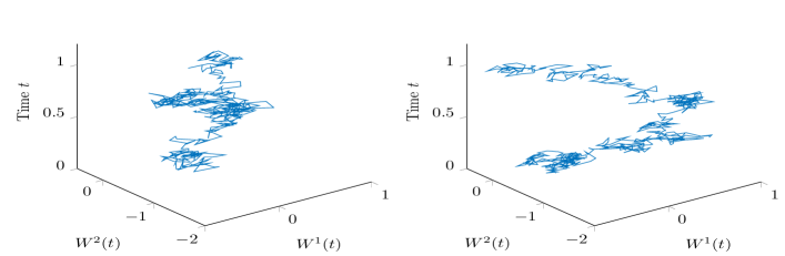
Figure 1. Two paths of a fractional Brownian motion with Hurst index $H=0.4$.

Simulations for the first path (left picture in Figure 1)

We compute a numerical approximation $\tilde{u}$ of the RPDE solution $u$ based on the pseudo-regression procedure, see Theorem 4.1, where for every fixed $t\in[0,1]$ the approximation $\tilde{u}(t,\cdot)$ is derived according to (4.10) and (4.11). We start with the left driver in Figure 1. Within the numerical approximation we encounter three different errors. The regression error itself depends on the number of basis functions $K$ and the number of samples $M$ that we use to approximate the expected value with respect to the probability measure $\mu$ of the initial data. In order to generate the paths of (5.1) that we require for the regression approach, we need to apply the Euler scheme from Section 5. The error in this discretization depends on the step size $h$ which is our third parameter.

We choose $\mu$ to be the uniform measure on $[0,1]^{2}$ and zero elsewhere. Based on this we choose Legendre polynomials on $[0,1]^{2}$ as an ONB $\left(\psi_{i}\right)_{i=1,\ldots,K}$ of $L^{2}(\mathbb{R}^{2},\mu)$. To be more precise, we consider the Legendre polynomials up to a certain fixed order $p$ for every spatial direction and then take into account the total tensor product between the basis functions of different spatial variables, such that $K=(p+1)^{n}$.

In Figure 2 we plot the regression solution $\tilde{u}$ on $[0,1]^{2}$ for three different time points. Here, we use $K=36$ Legendre polynomials, $M=10^{6}$ samples and a step size $h=2^{-9}$ of the Euler scheme (5.2). We observe in our simulations that $\tilde{u}$ is a very good approximation for the reference solution $u$ for these fixed parameters. The plots for $u$ look exactly as in Figure 2. Since there is no visible difference between $u$ and $\tilde{u}$, we omit the pictures for $u$.

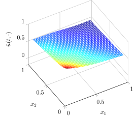
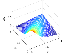
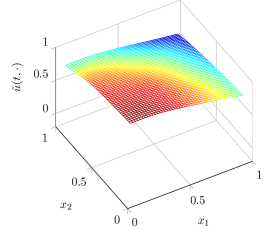
Figure 2. Pseudo-regression solution $\tilde{u}(t,\cdot)$, $t=0,0.84,0.99$, of the RPDE driven by the left path in Figure 1. The parameters are $K=36$, $h=2^{-9}$, $M=10^{6}$.

Below, we investigate how sensitive the pseudo-regression approach is in every single parameter. Therefore, we always fix two parameters and vary the remaining third one. All the errors are measured in $L^{2}([0,1]^{2})$, i.e., we compute $\left\|u(t,\cdot)-\tilde{u}(t,\cdot)\right\|_{L^{2}([0,1]^{2})}$, $t\in[0,1]$, or the corresponding relative error. In Figure 3, the absolute and relative errors are shown for different step sizes $h=2^{-7},2^{-8},2^{-9}$. If we compare the curves with the largest step size with the ones having the smallest step size, we can see that there is a remarkable difference. We observe that the error is most of the times twice and sometimes up to three time larger when using a four times larger step size. This can lead to an relative approximation error of more than $10\%$. This implies that a small step size $h$ is recommended in order to ensure a small error. This is not surprising since the order of convergence in $h$ is worst out of all parameters.

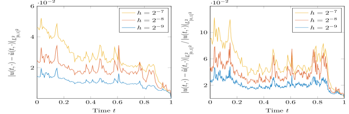
Figure 3. Absolute and relative error between RPDE and pseudo-regression solution. The parameters are $K=36$, $M=10^{6}$ and $h=2^{-7},2^{-8},2^{-9}$.

Now we fix the number of basis functions and the step size of the Euler method. For different numbers of samples $M=10^{4},10^{5},10^{6}$, we find the errors in Figure 4. We see that it does not really matter whether $10^{6}$ or $10^{5}$ samples are used, whereas $10^{4}$ samples are probably too few, since the relative error can be up to $9\%$.

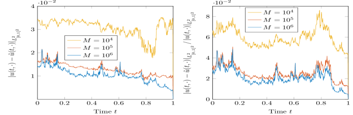
Figure 4. Absolute and relative error between RPDE and pseudo-regression solution. The parameters are $K=36$, $M=10^{4},10^{5},10^{6}$ and $h=2^{-9}$.

It remains to analyze the error in the number of basis functions. In Figure 2, the solution looks relatively flat, such that it is not surprising that the parameter $K$ only plays a minor role. Since there is barely a difference when varying $K$, we state the logarithmic errors in Figure 5 for $K=16,81$. The error for $K=36$ lies between the curves in Figure 5 and is omitted because it would have been hard to distinguish between the plots if it would have been included. Even in the logarithmic scale there is almost no difference in the errors. Moreover, we observe that for most of the time points, an additional error is caused by taking too many polynomials. Thus, the approach is not at all sensitive in the parameter $K$ for this problem with the left driving path in Figure 1. This is not true for every driving path as the following experiment will show. Using the right path in Figure 1 as the driver instead will lead to a much larger error if we choose the same parameters as before.

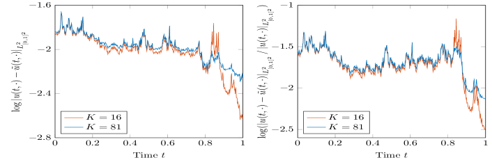
Figure 5. Logarithmic absolute and relative error between RPDE and pseudo-regression solution. The parameters are $K=16,81$, $M=10^{6}$ and $h=2^{-9}$.

Simulations for the second path (right picture in Figure 1)

We conduct a second experiment with the same example as above. We only change the driving path, i.e., the left path in Figure 1 is replaced by the right one. This leads to a very large relative $L^{2}$-error for $M=10^{6}$, $h=2^{-9}$ and $K=36$, see Figure 7. In the worst case ($t=0.48$) the relative error is almost $80\%$. The reason for this can be seen in Figure 6, where $u(0.48,\cdot)$ (left) is compared with $\tilde{u}(0.48,\cdot)$ (right). The exact solution in this worst case is close to be a delta function which is generally hard to approximate. The pseudo-regression solution clearly looks differently which shows that the parameter $K$ depends on the underlying driving path. If we increase the number of polynomials to $K=121$, we can reduce the error in Figure 7 but still many more basis functions would be required to obtain a small relative error which is still large at every time point, where $u$ is close to be a delta function.

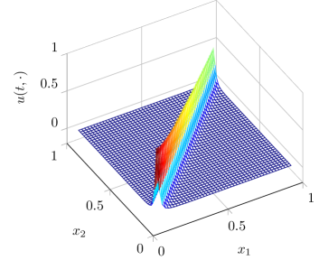
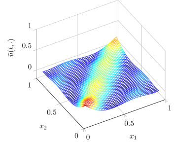
Figure 6. Exact solution $u(t,\cdot)$ (left) and pseudo-regression solution $\tilde{u}(t,\cdot)$ (right), $t=0.48$, of the RPDE driven by the right path in Figure 1 (coefficients as in (6.2)). The regression parameters are $K=36$, $h=2^{-9}$, $M=10^{6}$.

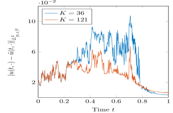
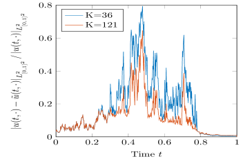
Figure 7. Absolute and relative error between RPDE and pseudo-regression solution with parameters $M=10^{6}$, $h=2^{-9}$ and $K=36,121$.

6.1.3. Numerical example with nilpotent matrices

In Subsection 6.1.2 an example has been considered that does not depend on the complete rough path but only on the path. Therefore, we investigate another case, where still a reference solution can be derived but this time it depends on the full rough path.

Let us consider an scenario that fits the framework (6.8). We set $b,c,\gamma\equiv 0$ in system (2.1) with terminal time $T=1$ and terminal value $g(x)=\exp\left(-0.5\left\|x\right\|^{2}\right)$. Moreover, we define

(6.9) $$\sigma(x)=A_{1}x,\;\;\;\beta_{1}(x)=A_{2}x\;\;\;\text{and}\;\;\;\beta_{2}(x)=A_{3}x,$$

where we assume $m=1$, $d=2$ and a three-dimensional space variable $x\in\mathbb{R}^{3}$. Again, by Theorem 2.1, the solution to (2.1) has the following stochastic representation:

(6.10) $$u(t,x;\mathbf{W})=E\left[g(X_{1}^{t,x})\right],\quad(t,x)\in[0,1]\times\mathbb{R}^{3},$$

where $X_{1}^{t,x}$ satisfies the RDE

(6.11) $$dX_{r}=A_{1}X_{r}dB_{r}+A_{2}X_{r}\mathbf{W}^{1}_{r}+A_{3}X_{r}\mathbf{W}^{2}_{r},\quad X_{t}=x,\quad r\in[t,1].$$

Now we fix the coefficients such that (6.8) is fulfilled:

$$A_{1}=\left(\begin{matrix}0&0&1\\ 0&0&0\\ 0&0&0\end{matrix}\right),\quad A_{2}=\left(\begin{matrix}0&1&0\\ 0&0&0\\ 0&0&0\end{matrix}\right),\quad A_{3}=\left(\begin{matrix}0&0&0\\ 0&0&1\\ 0&0&0\end{matrix}\right).$$

Notice that $A_{1}^{2}=0$ implies that the Itô-Stratonovich correction term is zero in (6.11) such that we automatically obtain a geometric driver in the equation. The driving path is again a fractional Brownian motion with Hurst index $H=0.4$. Now, since $A_{1}$ commutes with $A_{2}$ and $A_{3}$ it can be seen that $\ [A_{1},A_{2}]=\ [A_{1},A_{3}]=0$. Furthermore, we observe that $\ [A_{2},A_{3}]=A_{1}$ which by Lemma 6.1 leads to the following solution representation:

$$X_{r}^{t,x}=\exp\left(A_{1}(B_{t,r}-a^{12}_{t,r})+A_{2}W^{1}_{t,r}+A_{3}W^{2}_{t,r}\right)x,$$

where the term

$$a^{12}_{t,r}=\frac{1}{2}\left(\int_{t}^{r}W^{1}_{t,s}dW^{2}_{s}-\int_{t}^{r}W^{2}_{t,s}dW^{1}_{s}\right)$$

is approximated numerically by using piece-wise linear approximations to $W^{1}$ and $W^{2}$ on a very fine time grid. Consequently, we have

$$X_{r}^{t,x}=\exp\left(\begin{smallmatrix}0&W^{1}_{t,r}&B_{t,r}-a^{12}_{t,r}\\ 0&0&W^{2}_{t,r}\\ 0&0&0\end{smallmatrix}\right)x=:\exp\left(D_{t,r}\right)x.$$

The matrix $D_{t,r}$ is nilpotent with index $3$, so that $\exp\left(D_{t,r}\right)=I+D_{t,r}+\frac{1}{2}D_{t,r}^{2}$ which then leads to

$$X_{r}^{t,x}=\left(\begin{smallmatrix}1&W^{1}_{t,r}&B_{t,r}-a^{12}_{t,r}+0.5W^{1}_{t,r}W^{2}_{t,r}\\ 0&1&W^{2}_{t,r}\\ 0&0&1\end{smallmatrix}\right)x.$$

Inserting this into (6.10) and estimating the expected value with numerical integration provides the exact solution $u$ of the underlying RPDE.

The probability measure within the regression approach has the same structure as before but it is now defined on $\mathbb{R}^{3}$, i.e., we choose $\mu$ to be the uniform measure on $[0,1]^{3}$ and zero elsewhere. So, the ONB of $L^{2}(\mathbb{R}^{3},\mu)$ is given by Legendre polynomials on $[0,1]^{3}$. In Figure 8, the absolute and the relative error in $L^{2}([0,1]^{3})$ between the exact and the pseudo-regression solution is considered. The algorithm also works very well in this case since the relative error is less than $1\%$ for $K=64$ basis polynomials, $M=10^{6}$ samples and a Euler step size of $h=2^{-9}$.

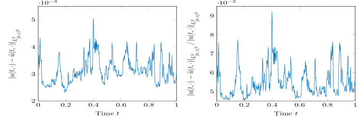
Figure 8. Absolute and relative error between the RPDE with coefficients as in (6.9) and the pseudo-regression solution. The parameters are $K=64$, $M=10^{6}$ and $h=2^{-9}$.

The pseudo-regression $\tilde{u}$ for several fixed time points is illustrated in Figure 9. In the cubic domain the color represents the corresponding function value of $\tilde{u}(t,\cdot)$ which is relatively large if the color is red and relatively small if the color is blue. We omit the plots for the exact solution since there is no visible difference to the regression solution.

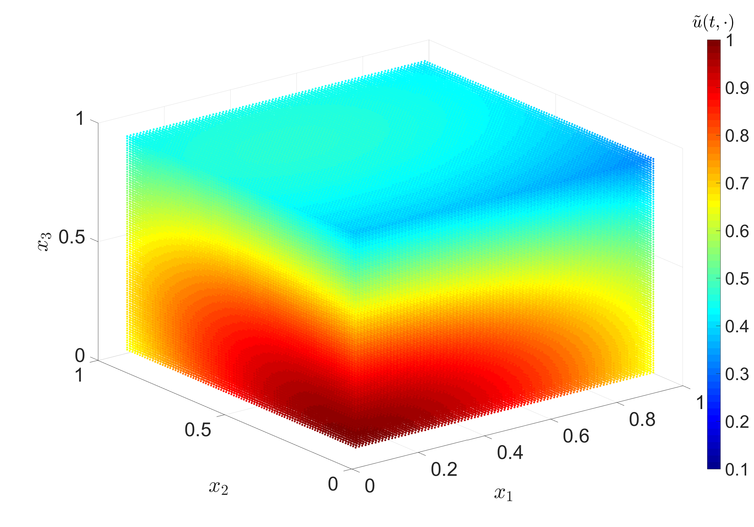
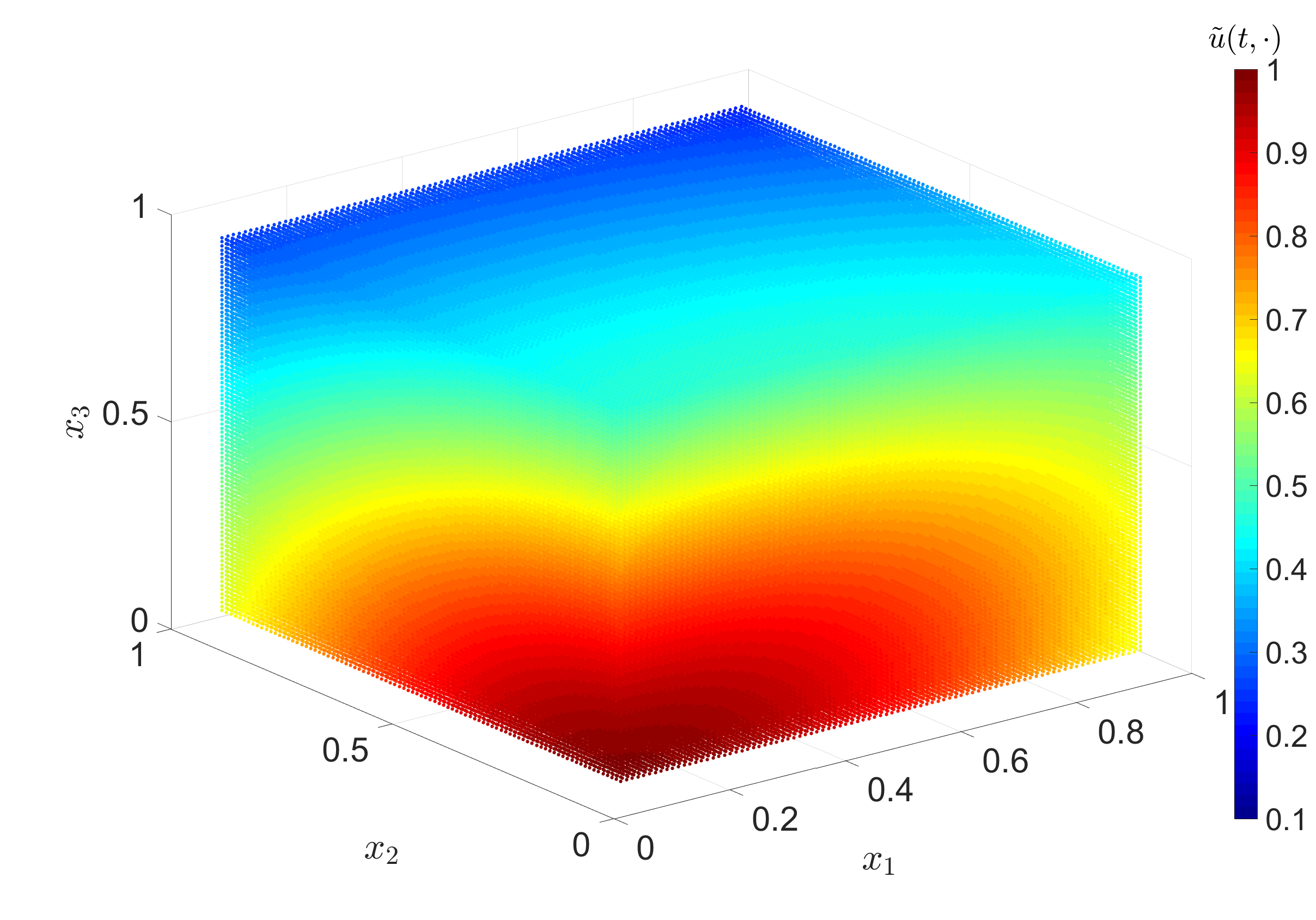
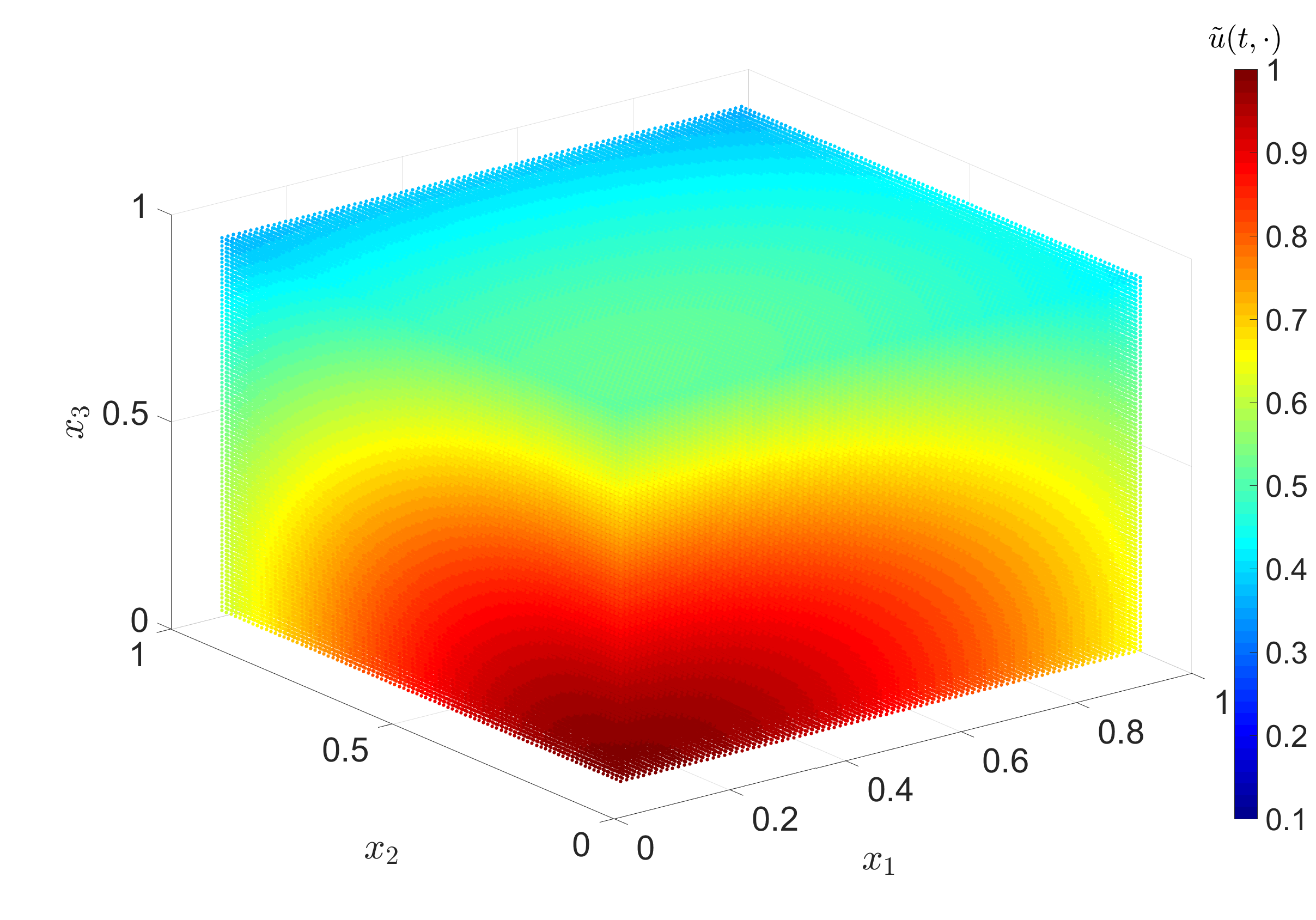
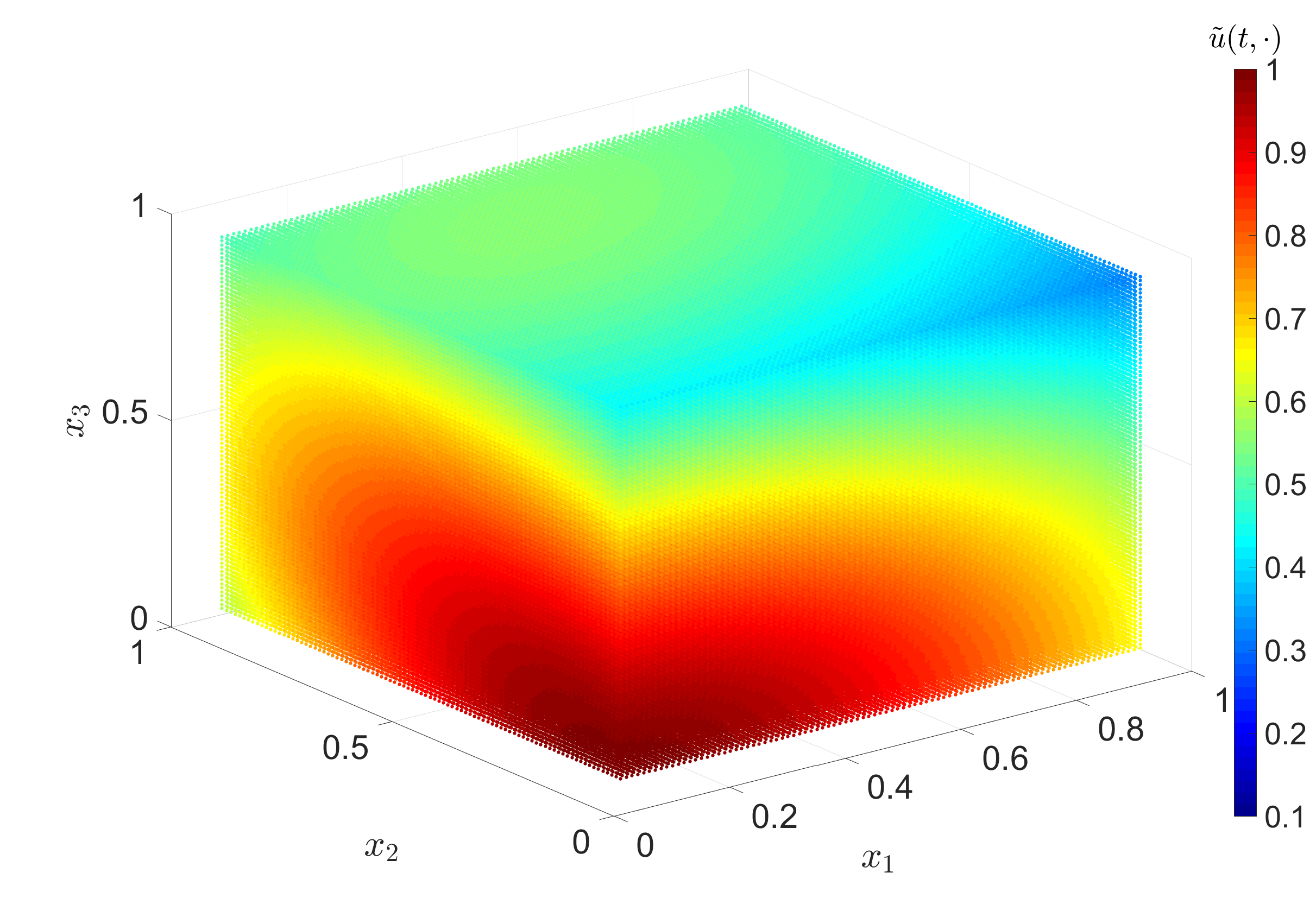
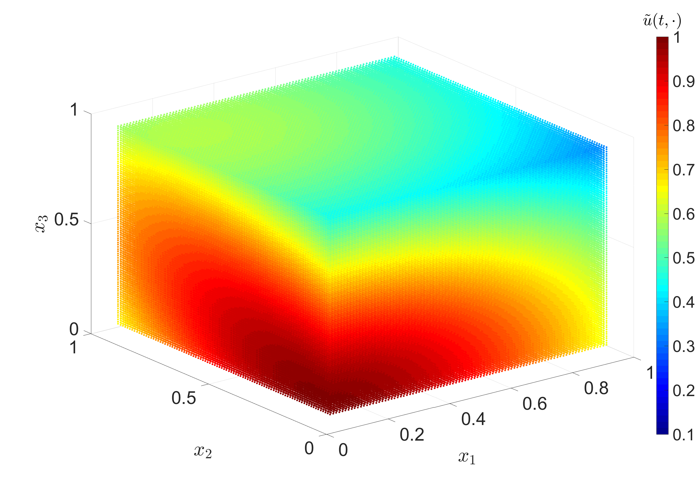
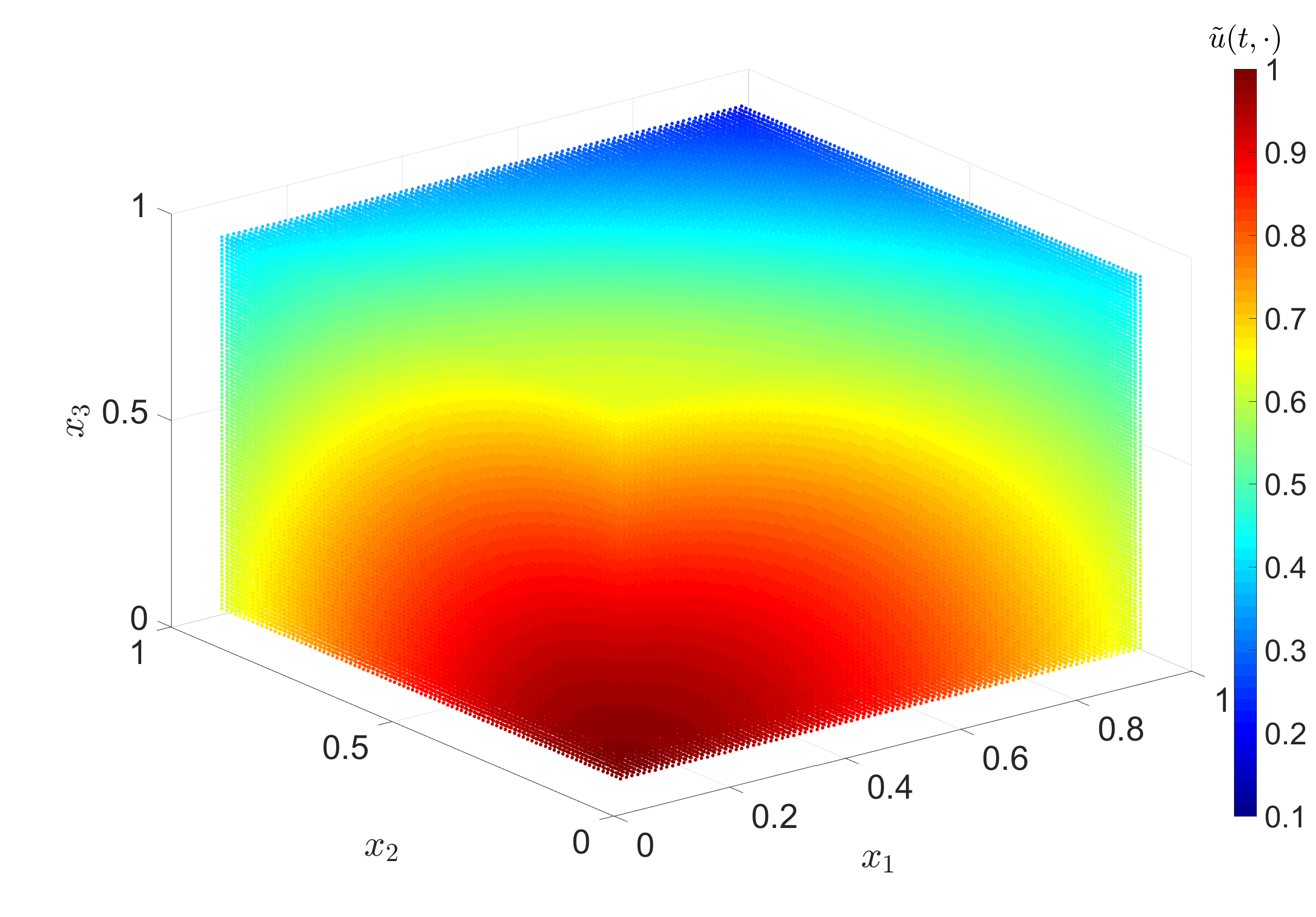
Figure 9. The pseudo-regression solution $\tilde{u}(t,\cdot)$, $t=0,0.14,0.43,0.61,0.78,0.99$, of the RPDE driven a path of a fBm. The parameters are $K=64$, $h=2^{-9}$, $M=10^{6}$.

We conclude this section by discussing an alternative to the pseudo-regression, that is the stochastic regression, where an approximation $\widehat{u}(t,\cdot)$ to $u(t,\cdot)$ is derived based on (4.7) instead of (4.11). Within the stochastic regression the Euler scheme (5.2) has to be used only once, whereas we run (5.2) for every fixed $t$ when computing the pseudo-regression solution $\tilde{u}(t,\cdot)$. Consequently, $\widehat{u}$ can be computationally cheaper than $\tilde{u}$ if the Euler method is very expensive in terms of computational time. We determine the solution of the stochastic regression $\widehat{u}$ with the same paprameters as before and compare it with the exact solution in Figure 10. In this context, we modify our basis, i.e., we use $\tilde{\psi}_{i}=g\psi_{i}$, where $\psi_{i}$ are again Legendre polynomials ($i=1,\ldots,K$). This compensation is required since $\psi_{i}$ takes very large values outside $[0,1]^{3}$. Now, we evaluate the basis functions at samples of the solution to (5.1) in order to compute $\mathcal{M}^{(t)}$ in (4.7). Since the paths of the solution to (5.1) leave $[0,1]^{3}$ quite frequently, we would encounter a very large variance and hence a large error when using the non-modified basis. With the basis $(\tilde{\psi}_{i})_{i=1,\ldots,K}$ we see that the error in Figure 10 is relatively small but it is clearly larger than the error of the pseudo-regression in Figure 8.

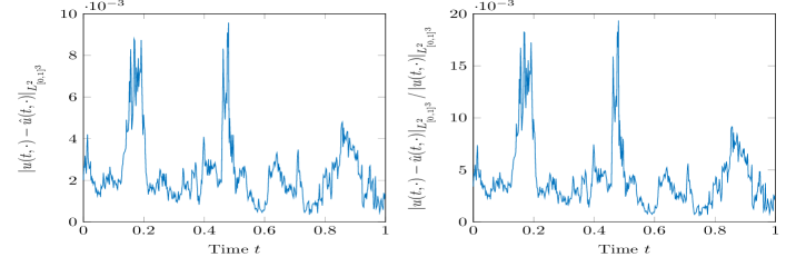
Figure 10. Absolute and relative error between the RPDE with coefficients as in (6.9) and the stochastic regression solution $\widehat{u}$. The parameters are as in Figure 8, i.e., $K=64$, $M=10^{6}$ and $h=2^{-9}$.

6.2. Numerical example with non-linear vector fields

We conclude the numerical section with an example which has no reference solution. We start with a similar setting as in Section 6.1, i.e., we assume that $c,\gamma\equiv 0$. Hence, the solution of the underlying RPDE is given by the expected value in (6.1) but here non-linear vector fields enter equation (5.1). We define them as follows:

(6.12) $$b(x)=\left(\begin{smallmatrix}\sin(x_{1}+2x_{2})\\ \sin(2x_{1}+x_{2})\end{smallmatrix}\right),\;\;\;\sigma(x)=\left(\begin{smallmatrix}x_{1}+\sin(x_{2})\\ 2x_{1}+0.5\cos(x_{2})\end{smallmatrix}\right),\;\;\;\beta(x)=\left(\begin{smallmatrix}0.3\cos(x_{1}+x_{2})&0.2(x_{1}+x_{2})\\ \sin(x_{2})-0.5x_{1}&\sin(x_{1}x_{2})-0.5x_{2}\end{smallmatrix}\right),$$

where we suppose to have a scalar Brownian motion $B$ ($m=1$), a two-dimensional spaces variable $x=\left(\begin{smallmatrix}x_{1}\\ x_{2}\end{smallmatrix}\right)\in\mathbb{R}^{2}$ as well as a two dimensional rough path $\mathbf{W}$ ($n=d=2$). Moreover, the terminal time and the terminal value of the RPDE are $T=1$ and $g(x)=\exp\left(-0.5\left\|x\right\|^{2}\right)$, respectively. We fix the probability measure $\mu$ like in Subsection 6.1.2 such that the ONB is again represented by Legendre polynomials on $[0,1]^{2}$. We apply the pseudo-regression approach to this case and illustrate the resulting solution $\tilde{u}$ in Figure 11 for $K=36,h=2^{-8}$ and $M=10^{6}$. Although there is no reference solution to determine the exact error, we expect the approximation to be good because $\tilde{u}$ is relatively flat in space and does not show an extreme behavior like in Figure 6.

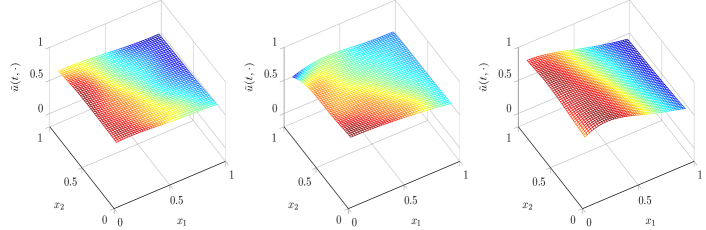
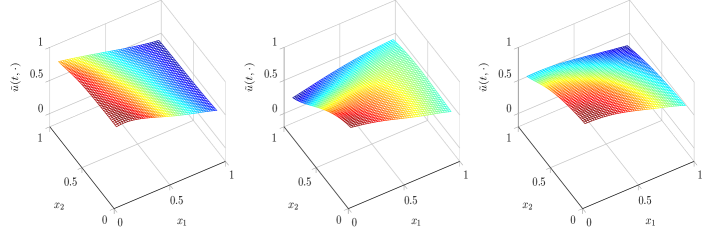
Figure 11. The pseudo-regression solution $\tilde{u}(t,\cdot)$, $t=0,0.33,0.57,0.73,0.87,0.99$, of the RPDE (vector fields as in (6.12)) driven by a path of a fBm with $H=0.4$. The regression parameters are $K=36,h=2^{-8}$ and $M=10^{6}$.

Appendix A Proof of Theorem 3.1

A.1. Controlled $p$-variation paths

Recall that a function

$$\omega\colon\{0\leq s\leq t\leq T\}\to[0,\infty)$$

is called control if it is continuous, $\omega(t,t)=0$ for all $t\in[0,T]$ and if it is superadditive, i.e.

$$\omega(s,u)+\omega(u,t)\leq\omega(s,t)$$

for all $s\leq u\leq t$. Examples of a control include $\omega(s,t)=|t-s|$ or $\omega(s,t)=\|\mathbf{Z}\|_{p-\text{var};[s,t]}^{p}$ provided $\mathbf{Z}$ is a $p$-rough path. We say that the $p$-variation of $\mathbf{Z}$ is controlled by a control function $\omega$ if $|\mathbf{Z}_{s,t}|^{p}\leq\omega(s,t)$ holds for all $s\leq t$. For arbitrary control functions, the quantity $N_{\alpha}(\omega;[s,t])$ is defined exactly as in (3.2) by replacing $\|\mathbf{Z}\|_{p-\text{var};[u,v]}^{p}$ by $\omega(u,v)$.

The following definition generalizes the notion of a controlled path from Hölder- to $p$-variation rough paths.

Definition A.1.

Let $U$ and $W$ be normed spaces. Let $Z\colon[0,T]\to U$ be a path whose $p$-variation is controlled by a control function $\omega$. We say that a path $y\colon[0,T]\to W$ is controlled by $Z$ and $\omega$ if there exists a path $y^{\prime}\colon[0,T]\to L(U,W)$ whose $p$-variation is controlled by $\omega$ so that for $R^{y}$ given implicitly by the relation

$$y_{s,t}=y^{\prime}_{s}Z_{s,t}+R^{y}_{s,t},$$

we have

$$\|R^{y}\|_{p/2-\omega;[0,T]}\coloneqq\sup_{0\leq s<t\leq T}\frac{|R^{y}_{s,t}|}{\omega(s,t)^{\frac{2}{p}}}<\infty.$$

We will usually not explicitly mention the control $\omega$ and just say that $y$ is controlled by $Z$. We denote by $\mathscr{D}_{Z}^{p}([0,T],W)$ the space of controlled $p$-rough paths. We will call a function $y^{\prime}$ with the given property a Gubinelli-derivative of $y$ (with respect to $Z$).

It is an (admittedly lengthy) exercise to show that all classical estimates proven for Hölder rough paths can be generalized to $p$-rough paths and their controlled functions in the sense above for $p\in[2,3)$ when replacing $|t-s|$ by $\omega(s,t)$ in these estimates. Indeed, the results follow by using an appropriate version of the Sewing Lemma for control functions which was proven recently, even for discontinuous control functions, in [18, Theorem 2.2]. For instance, the corresponding results for rough integrals are summarized in the following theorem.

Theorem A.2.

Let $U,W,\widehat{W}$ be finite dimensional vector spaces and $\mathbf{Z}=(Z,\mathbb{Z})$ be a $p$-rough path with $p$-variation controlled by $\omega$, $p\in[2,3)$. Let $y\in\mathscr{D}_{Z}^{p}([0,T],L(W,\widehat{W}))$ and $z\in\mathscr{D}_{Z}^{p}([0,T],W)$. Then

$$\int_{s}^{t}y_{u}\,dz_{u}=(\mathcal{I}\Xi)_{s,t}\ ,\qquad\Xi_{u,v}=y_{u}z_{u,v}+y^{\prime}_{u}z^{\prime}_{u}\mathbb{Z}_{u,v}$$

exists as an abstract integral (cf. [14, Lemma 4.2 and p. 49 eq. (4.6)]), and there is a constant $C$ depending only on $p$ such that the estimate

$$\left|\int_{s}^{t}y_{u}\,dz_{u}-y_{s}z_{s,t}-y^{\prime}_{s}z^{\prime}_{s}\mathbb{Z}_{s,t}\right|$$

$$\quad\leq C\left(\|x\|_{p-\omega;[s,t]}\|R^{z}\|_{p/2-\omega;[s,t]}+\|\mathbb{Z}\|_{p/2-\omega;[s,t]}\|y^{\prime}z^{\prime}\|_{p-\omega;[s,t]}\right)\omega(s,t)^{3/p}$$

holds for every $s<t$. In particular, the map $t\mapsto\int_{0}^{t}y_{u}\,dz_{u}$ is itself a controlled $p$-rough path, both controlled by $z$ with derivative $y$, and by $Z$ with derivative $yz^{\prime}$.

Proof.

A combination of [14, Theorem 4.10 and Remark 4.11] generalized to $p$-rough paths. ∎

In the next lemmas, we prepare some estimates for rough integrals and solutions to rough differential equations we are going to use at the end of this section. In the following, $U,W,\widehat{W},W_{1},W_{2},\ldots$ will denote finite dimensional vector spaces, and $\mathbf{Z}$ will be a fixed weakly geometric $p$-rough path, $p\in[2,3)$, with values in $U\oplus(U\otimes U)$, controlled by a control function $\omega$. $C\geq 0$ will denote a generic constant whose actual value may change from line to line and which might depend on the parameters specified before.

Lemma A.3.

Let $V\colon W\to L(U,W)$ and let $y\colon[0,T]\to W$ be a solution to

(A.1) $$y_{t}=x+\int_{0}^{t}V(y_{s})\,d\mathbf{Z}_{s}.$$

Assume that

$$\|y\|_{p-\omega}\vee\|\mathbf{Z}\|_{p-\omega}\leq 1\quad\text{and}\quad\|V\|_{\mathcal{C}^{2}_{b}}\leq 1.$$

Then there are constants $C$ and $\alpha$ depending only on $p$ such that

$$\|R^{y}\|_{p/2-\omega}\leq C(1+N_{\alpha}(\omega;[0,T])).$$

Proof.

For $\alpha>0$, set

$$\|R^{y}\|_{p/2-\omega;\alpha}:=\sup_{0\leq s<t\leq T;|t-s|\leq\alpha}\frac{|R^{y}_{s,t}|}{\omega(s,t)^{2/p}}.$$

Choose $s<t$ such that $\omega(s,t)\leq\alpha$. Then we have, using the estimate in Theorem A.2,

$$|R^{y}_{s,t}| =\left|\int_{s}^{t}V(y_{u})\,d\mathbf{Z}_{u}-V(y_{s})Z_{s,t}\right|$$

$$\leq\left|\int_{s}^{t}V(y_{u})\,d\mathbf{Z}_{u}-V(y_{s})Z_{s,t}-DV(y_{s})V(y_{s})\mathbb{Z}_{s,t}\right|+|DV(y_{s})V(y_{s})\mathbb{Z}_{s,t}|$$

$$\leq C\alpha^{1/p}\omega(s,t)^{2/p}(\|R^{y}\|_{p/2-\omega;\alpha}+\|DV(y_{\cdot})V(y_{\cdot})\|_{p-\omega})+\omega(s,t)^{2/p}.$$

Using boundedness of $V$ and its derivatives, one can check that

$$\|DV(y_{\cdot})V(y_{\cdot})\|_{p-\omega}\leq C\|y\|_{p-\omega}\leq C.$$

Hence we obtain

$$\|R^{y}\|_{p/2-\omega;\alpha}\leq C\alpha^{1/p}\|R^{y}\|_{p/2-\omega;\alpha}+C.$$

Choosing $\alpha$ such that $C\alpha^{1/p}\leq 1/2$, we obtain

$$\|R^{y}\|_{p/2-\omega;\alpha}\leq 2C.$$

Now choose $(\tau_{n})$ such that $0=\tau_{0}<\tau_{1}<\ldots<\tau_{N}<\tau_{N+1}=T$ with $\omega(\tau_{i},\tau_{i+1})\leq\alpha$ and $N=N_{\alpha}(\omega;[0,T])$. Let $s<t$ be arbitrary. Choose $i$ and $j$ such that $s\in[\tau_{i-1},\tau_{i})$ and $t\in(\tau_{j},\tau_{j+1}]$. Then

$$\frac{|R^{y}_{s,t}|}{\omega(s,t)^{2/p}} \leq\omega(s,t)^{-2/p}\big{(}|R^{y}_{s,\tau_{i}}|+|R^{y}_{\tau_{i},\tau_{i+1}}|+\ldots+|R^{y}_{\tau_{j},t}|$$

$$\quad+|V(y_{\tau_{i}})-V(y_{s})||Z_{\tau_{i},\tau_{i+1}}|+\ldots+|V(y_{\tau_{j}})-V(y_{s})||Z_{\tau_{j},t}|\big{)}$$

$$\leq\frac{|R^{y}_{s,\tau_{i}}|}{\omega(s,\tau_{i})^{2/p}}+\ldots+\frac{|R^{y}_{\tau_{j},t}|}{\omega(\tau_{j},t)^{2/p}}+\frac{|V(y_{\tau_{i}})-V(y_{s})||Z_{\tau_{i},\tau_{i+1}}|}{\omega(s,\tau_{i})^{1/p}\omega(\tau_{i},\tau_{i+1})^{1/p}}+\ldots+\frac{|V(y_{\tau_{j}})-V(y_{s})||Z_{\tau_{j},t}|}{\omega(s,\tau_{j})^{1/p}\omega(\tau_{j},t)^{1/p}}$$

$$\leq 2C(N_{\alpha}(\omega;[0,T])+1)+C(N_{\alpha}(\omega;[0,T])+1).\qed$$

Lemma A.4.

Let $y$ be a solution to (A.1). Consider

$$\zeta_{t}=\zeta_{0}+\int_{0}^{t}\nu(y_{s})(d\mathbf{Z}_{s})z_{s}\in L(\widehat{W},W)$$

where $\nu\colon W\to L(U,L(W_{1},W))$ is bounded, twice differentiable with bounded derivatives and $z\colon[0,T]\to L(\widehat{W},W_{1})$ is controlled by $Z$. Assume that

$$\|y\|_{p-\omega}\vee\|\mathbf{Z}\|_{p-\omega}\leq 1\quad\text{and}\quad\|\nu\|_{\mathcal{C}^{2}_{b}}\leq 1.$$

Then there is a constant $C$ and some $\alpha>0$ depending on $p$ such that

$$\|\zeta\|_{p-\omega;[s,t]} \leq C\omega(s,t)^{2/p}\Big{(}\|z\|_{\infty;[s,t]}(1+N_{\alpha}(\omega;[0,T]))+\|z\|_{\infty;[s,t]}+\|z^{\prime}\|_{\infty;[s,t]}$$

$$\quad+\|z\|_{p-\omega;[s,t]}+\|z^{\prime}\|_{p-\omega;[s,t]}+\|R^{z}\|_{p/2-\omega;[s,t]}\Big{)}$$

$$\quad+C\omega(s,t)^{1/p}(\|z\|_{\infty;[s,t]}+\|z^{\prime}\|_{\infty;[s,t]})+C\|z\|_{\infty;[s,t]}$$

and

$$\|R^{\zeta}\|_{p/2-\omega;[s,t]} \leq C\omega(s,t)^{1/p}\Big{(}\|z\|_{\infty;[s,t]}(1+N_{\alpha}(\omega;[0,T]))+\|z\|_{\infty;[s,t]}+\|z^{\prime}\|_{\infty;[s,t]}$$

$$\quad+\|z\|_{p-\omega;[s,t]}+\|z^{\prime}\|_{p-\omega;[s,t]}+\|R^{z}\|_{p/2-\omega;[s,t]}\Big{)}+C(\|z\|_{\infty;[s,t]}+\|z^{\prime}\|_{\infty;[s,t]})$$

for all $s\leq t$.

Proof.

Note first that the path $t\mapsto y_{t}$ is controlled by $Z$, and the path $t\mapsto\nu(y_{t})z_{t}\in L(U,L(\widehat{W},W))$ is controlled by $Z$ as composition with a smooth function [14, Lemma 7.3]. Moreover, its Gubinelli derivative is given by

$$(\nu(y_{t})z_{t})^{\prime}=(\nu(y_{t}))^{\prime}z_{t}+\nu(y_{t})z_{t}^{\prime}=D\nu(y_{t})(y^{\prime}_{t})z_{t}+\nu(y_{t})z_{t}^{\prime}=D\nu(y_{t})V(y_{t})z_{t}+\nu(y_{t})z_{t}^{\prime}$$

where we used ($p$-variation versions of) [14, Lemma 7.3] in the first and second equality and [14, Theorem 8.4] in the third. We start to prove the claimed estimate for $R^{\zeta}$. The Gubinelli derivative of $\zeta$ is given by $\zeta_{t}^{\prime}=\nu(y_{t})z_{t}$ and

$$R^{\zeta}_{s,t}=\int_{s}^{t}\nu(y_{u})(d\mathbf{Z}_{u})z_{u}\,-\nu(y_{s})(z_{s})Z_{s,t}.$$

Hence we can estimate

$$|R^{\zeta}_{s,t}| \leq\left|\int_{s}^{t}\nu(y_{u})(d\mathbf{Z}_{u})z_{u}-\nu(y_{s})(z_{s})Z_{s,t}-(\nu(y_{s})z_{s})^{\prime}\mathbb{Z}_{s,t}\right|+\left|D\nu(y_{s})V(y_{s})z_{s}\mathbb{Z}_{s,t}+\nu(y_{s})z_{s}^{\prime}\mathbb{Z}_{s,t}\right|$$

$$\leq C\left(\|R^{\nu(y_{\cdot})z_{\cdot}}\|_{p/2-\omega;[s,t]}+\|D\nu(y_{\cdot})V(y_{\cdot})z_{\cdot}\|_{p-\omega;[s,t]}+\|D\nu(y_{\cdot})z^{\prime}_{\cdot}\|_{p-\omega;[s,t]}\right)\omega(s,t)^{3/p}$$

$$\quad+C(\|z\|_{\infty;[s,t]}+\|z^{\prime}\|_{\infty;[s,t]})\omega(s,t)^{2/p}$$

where we used Theorem A.2 and that $V$, $\nu$ and all its derivatives are bounded. We have

$$|R^{\nu(y_{\cdot})z_{\cdot}}_{s,t}| =|\nu(y_{t})z_{t}-\nu(y_{s})z_{s}-(\nu(y_{s}))^{\prime}z_{s}Z_{s,t}-\nu(y_{s})z^{\prime}_{s}Z_{s,t}|$$

$$\leq|(\nu(y_{t})-\nu(y_{s})-(\nu(y_{s}))^{\prime}Z_{s,t})z_{t}|+|\nu(y_{s})(z_{t}-z_{s}-z^{\prime}_{s}Z_{s,t})|+|(\nu(y_{s}))^{\prime}(z_{t}-z_{s})Z_{s,t}|$$

$$\leq C(\|R^{\nu(y_{\cdot})}\|_{p/2-\omega;[s,t]}\|z\|_{\infty}+\|R^{z}\|_{p/2-\omega;[s,t]}+\|z\|_{p-\omega;[s,t]})\omega(s,t)^{2/p}$$

using $(\nu(y_{s}))^{\prime}=D\nu(y_{s})V(y_{s})$ and boundedness of the vector fields an their derivatives. As in [14, Lemma 7.3], we can see that

$$\|R^{\nu(y_{\cdot})}\|_{p/2-\omega;[s,t]} \leq C\left(\|y\|^{2}_{p-\omega;[s,t]}+\|R^{y}\|_{p/2-\omega;[s,t]}\right)$$

$$\leq C(1+N_{\alpha}(\omega;[0,T]))$$

where the second estimate follows from Lemma A.3. Thus

$$\|R^{\nu(y_{\cdot})z_{\cdot}}\|_{p-\omega;[s,t}\leq C(\|z\|_{\infty}(1+N_{\alpha}(\omega;[0,T]))+\|R^{z}\|_{p/2-\omega;[s,t]}+\|z\|_{p-\omega;[s,t]}).$$

Using the Lipschitz bounds for $V$, $\nu$ and its derivatives, we can easily see that

$$\|D\nu(y_{\cdot})V(y_{\cdot})z_{\cdot}\|_{p-\omega;[s,t]} \leq C(\|z\|_{\infty;[s,t]}+\|z\|_{p-\omega;[s,t]})\quad\text{and}$$

$$\|D\nu(y_{\cdot})z^{\prime}_{\cdot}\|_{p-\omega;[s,t]} \leq C(\|z^{\prime}\|_{\infty;[s,t]}+\|z^{\prime}\|_{p-\omega;[s,t]}).$$

Therefore, we find that

$$\|R^{\zeta}\|_{p/2-\omega;[s,t]} \leq C\omega(s,t)^{1/p}\big{(}\|z\|_{\infty;[s,t]}(1+N_{\alpha}(\omega;[0,T]))+\|z\|_{\infty;[s,t]}+\|z^{\prime}\|_{\infty;[s,t]}$$

$$\quad+\|z\|_{p-\omega;[s,t]}+\|z^{\prime}\|_{p-\omega;[s,t]}+\|R^{z}\|_{p/2-\omega;[s,t]}\big{)}+C(\|z\|_{\infty;[s,t]}+\|z^{\prime}\|_{\infty;[s,t]}).$$

For $\zeta$, we have

$$\frac{|\zeta_{s,t}|}{\omega(s,t)^{1/p}} \leq\omega(s,t)^{1/p}\frac{|R^{\zeta}_{s,t}|}{\omega(s,t)^{2/p}}+\frac{|\nu(y_{s})(z_{s})Z_{s,t}|}{\omega(s,t)^{1/p}}$$

$$\leq\omega(s,t)^{1/p}\|R^{\zeta}\|_{p/2-\omega;[s,t]}+C\|z\|_{\infty;[s,t]}$$

for all $s<t$ and the claim follows. ∎

Lemma A.5.

Let $A\colon[0,T]\to L(U,L(W,W))$ be controlled by $Z$, and let $\mathbf{Z}$ be weakly geometric. Consider a solution $\Phi\colon[0,T]\to L(W,W)$ to

$$\Phi_{t}=\Phi_{0}+\int_{0}^{t}A(s)(d\mathbf{Z}_{s})\Phi_{s}\in L(W,W).$$

Then Liouville’s formula holds:

$$\det(\Phi_{t})=\det(\Phi_{0})\exp\left(\operatorname{Tr}\int_{0}^{t}A(s)\,d\mathbf{Z}_{s}\right).$$

In particular, if $\det(\Phi_{0})\neq 0$, $\Phi_{t}$ is invertible for every $t\geq 0$. In this case, the inverse $\Psi_{t}:=\Phi_{t}^{-1}$ solves the equation

$$\Psi_{t}=\Phi_{0}^{-1}-\int_{0}^{t}\Psi_{s}A(s)(d\mathbf{Z}_{s})\in L(W,W).$$

Proof.

Assume first that $Z$ is smooth. In this case, Liouville’s formula is well-known, cf. [1, (11.4) Proposition]. The statement about $\Psi$ follows from the identity

$$\frac{d\Phi_{t}^{-1}}{dt}=-\Phi_{t}^{-1}\frac{d\Phi_{t}}{dt}\Phi_{t}^{-1},$$

which is true for matrices depending smoothly on $t$. The general case follows by approximation of $\mathbf{Z}$ with smooth rough paths and continuity of the rough integral. ∎

Lemma A.6.

Let $y$ be a solution to (A.1). Consider a solution $\Phi\colon[0,T]\to L(W,W)$ to

$$\Phi_{t}=\Phi_{0}+\int_{0}^{t}\nu(y_{u})(d\mathbf{Z}_{u})\Phi_{u}\in L(W,W)$$

where $\nu\colon W\to L(U,L(W,W))$ is bounded, twice differentiable and has bounded derivatives. Assume that

$$\|y\|_{p-\omega}\vee\|\mathbf{Z}\|_{p-\omega}\leq 1\quad\text{and}\quad\|\nu\|_{\mathcal{C}^{2}_{b}}\leq 1.$$

Then $\Phi$ is controlled by $Z$ and there are constants $C$ and $\alpha>0$ depending on $p$ such that

$$\|R^{\Phi}\|_{p/2-\omega} \leq C(1+|\Phi_{0}|)\exp(CN_{\alpha}(\omega;[0,T]))\quad\text{and}$$

$$\|\Phi\|_{\infty}+\|\Phi\|_{p-\omega}+\|\Phi^{\prime}\|_{\infty}+\|\Phi^{\prime}\|_{p-\omega} \leq C(1+|\Phi_{0}|)\exp(CN_{\alpha}(\omega;[0,T])).$$

The same estimate holds true for any solution $\Psi\colon[0,T]\to L(W,W)$ to

$$\Psi_{t}=\Psi_{0}-\int_{0}^{t}\Psi_{u}\nu(y_{u})(d\mathbf{Z}_{u})\in L(W,W)$$

when we replace $\Phi_{0}$ by $\Psi_{0}$.

Proof.

Note that $\Phi$ is controlled by $Z$ with derivative

(A.2) $$(\Phi_{t})^{\prime}=\nu(y_{t})\Phi_{t}.$$

Using boundedness of $\nu$ and its derivative and our assumptions on $\omega$, this implies that

$$\|\Phi^{\prime}\|_{\infty;[s,t]}\leq C\|\Phi\|_{\infty;[s,t]}\quad\text{and}\quad\|\Phi^{\prime}\|_{p-\omega;[s,t]}\leq C(\|\Phi\|_{p-\omega;[s,t]}+\|\Phi\|_{\infty;[s,t]})$$

for all $s<t$, therefore it is enough to bound $\Phi$ to obtain bounds for $\Phi^{\prime}$. Let $K$ be a constant such that

$$\|\Phi\|_{p-\omega;[0,T]}+\|\Phi\|_{\infty;[0,T]}\leq K.$$

Let $\alpha>0$ and choose $s<t$ such that $\omega(s,t)\leq\alpha$. Using Lemma A.4, we have for sufficiently small $\alpha$

$$\|R^{\Phi}\|_{p/2-\omega;[s,t]}\leq C\alpha^{1/p}\|R^{\Phi}\|_{p/2-\omega;[s,t]}+C\alpha^{1/p}K(1+N_{\alpha}(\omega;[0,T]))+CK.$$

Choosing $\alpha$ smaller if necessary, we may assume that $C\alpha^{1/p}\leq 1/2$ and we therefore obtain

$$\|R^{\Phi}\|_{p/2-\omega;[s,t]}\leq 2C\alpha^{1/p}K(1+N_{\alpha}(\omega;[0,T]))+2CK\leq CK(1+N_{\alpha}(\omega;[0,T])).$$

Using the same strategy as at the end of the proof of Lemma A.3, we can conclude that

$$\|R^{\Phi}\|_{p/2-\omega;[0,T]}\leq CK(1+N_{\alpha}(\omega;[0,T]))^{2}.$$

Using the results about linear rough differential equations in [15, Section 5], we see that we can choose

$$K=C(1+|\Phi_{0}|)\exp(CN_{\alpha}(\omega;[0,T]))$$

and the claim follows for $R^{\Phi}$. The estimates for $\Phi$ can either be obtained by a direct calculation similar to the one performed in Lemma A.4, but also follow from the results proven for linear rough differential equations in [15, Section 5]. The estimates for $\Psi$ can be obtained in exactly the same way. ∎

Lemma A.7.

Let $y$ be a solution to (A.1). Let $\zeta\colon[0,T]\to L(\widehat{W},W)$ be of the form

$$\zeta_{t}=\int_{0}^{t}\widehat{\nu}(y_{u})(d\mathbf{Z}_{u})\widehat{z}_{u}$$

for some $\widehat{\nu}\colon W\to L(U,L(W_{1},W))$ and $\widehat{z}\colon[0,T]\to L(\widehat{W},W_{1})$. Assume that $\widehat{z}$ is controlled by $Z$. Consider

$$z_{t}=\Phi_{t}\left(z_{0}+\int_{0}^{t}\Psi_{u}\,d\zeta_{u}\right),\quad z_{0}\in L(\widehat{W},W)$$

with $\Phi,\Psi$ as in Lemma A.6 where we assume in addition that $\Phi_{0}=\Psi_{0}=\operatorname{Id}$. Assume that

$$\|y\|_{p-\omega}\vee\|\mathbf{Z}\|_{p-\omega}\leq 1\quad\text{and}\quad\|\widehat{\nu}\|_{\mathcal{C}^{2}_{b}}\leq 1.$$

Let $\kappa\geq 1$ be a constant such that

$$\|\widehat{z}\|_{\infty}+\|\widehat{z}\|_{p-\omega}+\|\widehat{z}^{\prime}\|_{\infty}+\|\widehat{z}^{\prime}\|_{p-\omega}+\|R^{\widehat{z}}\|_{p/2-\omega}\leq\kappa.$$

Then $z$ is controlled by $Z$ and there are constants $C>0$ and $\alpha>0$ depending only on $p$ such that

$$\|z\|_{\infty}+\|z\|_{p-\omega}+\|z^{\prime}\|_{\infty}+\|z^{\prime}\|_{p-\omega}+\|R^{z}\|_{p/2-\omega}$$

$$\quad\leq C\kappa(1+|z_{0}|)(1+\omega(0,T)^{1/p}+\omega(0,T)^{4/p})\exp(CN_{\alpha}(\omega;[0,T])).$$

Proof.

It is clear that $z$ is controlled by $Z$, and the Gubinelli derivative is given by

(A.3) $$\begin{split}z^{\prime}_{t}&=\Phi^{\prime}_{t}\left(z_{0}+\int_{0}^{t}\Psi_{u}\,d\zeta_{u}\right)+\Phi_{t}(\Psi_{t}\zeta^{\prime}_{t})=\nu(y_{t})\Phi_{t}\left(z_{0}+\int_{0}^{t}\Psi_{u}\,d\zeta_{u}\right)+\widehat{\nu}(y_{t})\widehat{z}_{t}\\ &=\nu(y_{t})z_{t}+\widehat{\nu}(y_{t})\widehat{z}_{t}\end{split}$$

where we used Theorem A.2, $\zeta^{\prime}_{t}=\widehat{\nu}(y_{t})\widehat{z}_{t}$ and the fact that $\Psi_{t}=(\Phi_{t})^{-1}$. For $s<t$, we therefore obtain

$$R^{z}_{s,t} =z_{s,t}-z^{\prime}_{s}Z_{s,t}$$

$$=\Phi_{t}\int_{s}^{t}\Psi_{u}\,d\zeta_{u}+\Phi_{s,t}z_{s}-\nu(y_{s})(Z_{s,t})z_{s}-\widehat{\nu}(y_{s})(Z_{s,t})\widehat{z}_{s}$$

$$=\Phi_{t}\left(\int_{s}^{t}\Psi_{u}\,d\zeta_{u}-\Psi_{s}\zeta_{s,t}+\Psi_{s}R^{\zeta}_{s,t}\right)+\Phi_{t}\Psi_{s}\zeta^{\prime}_{s}Z_{s,t}+\Phi_{s,t}z_{s}-\Phi^{\prime}_{s}Z_{s,t}z_{s}-\widehat{\nu}(y_{s})(Z_{s,t})\widehat{z}_{s}$$

$$=\Phi_{t}\left(\int_{s}^{t}\Psi_{u}\,d\zeta_{u}-\Psi_{s}\zeta_{s,t}+\Psi_{s}R^{\zeta}_{s,t}\right)+R^{\Phi}_{s,t}z_{s}+(\Phi_{t}-\Phi_{s})\Psi_{s}\widehat{\nu}(y_{s})(Z_{s,t})\widehat{z}_{s}$$

and by the triangle inequality,

(A.4) $$\begin{split}|R^{z}_{s,t}|&\leq\left|\Phi_{t}\left(\int_{s}^{t}\Psi_{u}\,d\zeta_{u}-\Psi_{s}\zeta_{s,t}+\Psi_{s}R_{s,t}^{\zeta}\right)\right|+\left|R^{\Phi}_{s,t}\left(z_{0}+\int_{0}^{s}\Psi_{u}\,d\zeta_{u}\right)\right|\\ &\quad+|(\Phi_{t}-\Phi_{s})\Psi_{s}\widehat{\nu}(y_{s})(Z_{s,t})\widehat{z}_{s}|.\end{split}$$

For the first term on the right hand side in (A.4), we can use the estimate in Theorem A.2 to see that

$$\left|\Phi_{t}\left(\int_{s}^{t}\Psi_{u}\,d\zeta_{u}-\Psi_{s}\zeta_{s,t}+\Psi_{s}R_{s,t}^{\zeta}\right)\right|$$

$$\leq\ C\|\Phi\|_{\infty;[s,t]}\omega(s,t)^{2/p}\Big{(}(\|R^{\zeta}\|_{p/2-\omega;[s,t]}+\|\Psi^{\prime}\zeta^{\prime}\|_{p-\omega;[s,t]})\omega(s,t)^{1/p}+\|\Psi^{\prime}\|_{\infty;[s,t]}\|\zeta^{\prime}\|_{\infty;[s,t]}$$

$$\qquad+\|\Psi\|_{\infty;[s,t]}\|R^{\zeta}\|_{p/2-\omega;[s,t]}\Big{)}.$$

Note first that

$$\|\Psi^{\prime}\zeta^{\prime}\|_{p-\omega;[s,t]}\leq\|\Psi^{\prime}\|_{p-\omega;[s,t]}\|\zeta^{\prime}\|_{\infty;[s,t]}+\|\Psi^{\prime}\|_{\infty;[s,t]}\|\zeta^{\prime}\|_{p-\omega;[s,t]}$$

and

$$\|\zeta^{\prime}\|_{\infty}+\|\zeta^{\prime}\|_{p-\omega}\leq C\kappa.$$

From Lemma A.4, it follows that

$$\|R^{\zeta}\|_{p/2-\omega;[s,t]}\leq C\kappa\left(\omega(s,t)^{1/p}(1+N_{\alpha}(\omega;[0,T]))+1\right).$$

Using the estimates for $\Phi$ and $\Psi$ in Lemma A.6, we therefore obtain

$$\left|\Phi_{t}\left(\int_{s}^{t}\Psi_{u}\,d\zeta_{u}-\Psi_{s}\zeta_{s,t}+\Psi_{s}R_{s,t}^{\zeta}\right)\right|\leq C\kappa\omega(s,t)^{2/p}(1+\omega(0,T)^{1/p}+\omega(0,T)^{2/p})\exp(CN_{\alpha}(\omega;[0,T]))$$

for all $s<t$. For the second summand in (A.4), we can again use Theorem A.2 to estimate

$$\left|R^{\Phi}_{s,t}\left(z_{0}+\int_{0}^{s}\Psi_{u}\,d\zeta_{u}\right)\right| \leq C\omega(s,t)^{2/p}\|R^{\Phi}\|_{p/2-\omega;[s,t]}$$

$$\quad\times\Big{(}|z_{0}|+\omega(0,s)^{3/p}(\|R^{\zeta}\|_{p/2-\omega;[0,s]}+\|\Psi^{\prime}\zeta^{\prime}\|_{p-\omega;[0,s]})$$

$$\qquad+\|\zeta\|_{\infty;[0,s]}+\omega(0,s)^{2/p}|\widehat{z}_{0}|\Big{)}$$

using $\Psi_{0}=\operatorname{Id}$, $\Psi^{\prime}_{0}=\nu(y_{0})$ and $\zeta^{\prime}_{0}=\widehat{\nu}(y_{0})\widehat{z}_{0}$. With Lemma A.4, we obtain

$$\|\zeta\|_{\infty;[0,s]}\leq\omega(0,T)^{1/p}\|\zeta\|_{p-\omega}\leq C\kappa(\omega(0,T)^{1/p}+\omega(0,T)^{3/p})(1+N_{\alpha}(\omega;[0,T])).$$

As above, we obtain the bound

$$\left|R^{\Phi}_{s,t}\left(z_{0}+\int_{0}^{s}\Psi_{u}\,d\zeta_{u}\right)\right|\leq C\kappa\omega(s,t)^{2/p}(1+|z_{0}|)(1+\omega(0,T)^{1/p}+\omega(0,T)^{4/p})\exp(CN_{\alpha}(\omega;[0,T]))$$

for all $s<t$. For the third term in (A.4), we have

$$|(\Phi_{t}-\Phi_{s})\Psi_{s}\widehat{\nu}(y_{s})(Z_{s,t})\widehat{z}_{s}| \leq\kappa\omega(s,t)^{2/p}\|\Phi\|_{p-\omega;[s,t]}\|\Psi\|_{\infty;[0,s]}$$

$$\leq C\kappa\omega(s,t)^{2/p}\exp(CN_{\alpha}(\omega;[0,T])).$$

Using all these estimates in (A.4), we can conclude that

$$\|R^{z}\|_{p/2-\omega}\leq C\kappa(1+|z_{0}|)(1+\omega(0,T)^{1/p}+\omega(0,T)^{4/p})\exp(CN_{\alpha}(\omega;[0,T])).$$

We proceed with $z$. For $s<t$,

$$|z_{t}-z_{s}|\leq|\Phi_{t}|\left|\int_{s}^{t}\Psi_{u}\,d\zeta_{u}\right|+|\Phi_{t}-\Phi_{s}|\left|z_{0}+\int_{0}^{s}\Psi_{u}\,d\zeta_{u}\right|$$

and as before, we obtain the estimate

$$\|z\|_{p-\omega}\leq C\kappa(1+|z_{0}|)(1+\omega(0,T)^{1/p}+\omega(0,T)^{4/p})\exp(CN_{\alpha}(\omega;[0,T])).$$

Similarly,

$$\|z\|_{\infty}\leq C\kappa(1+|z_{0}|)(1+\omega(0,T)^{1/p}+\omega(0,T)^{4/p})\exp(CN_{\alpha}(\omega;[0,T])).$$

From (A.3), we see that

$$\|z^{\prime}\|_{\infty;[s,t]}\leq C(\|z\|_{\infty;[s,t]}+\|\widehat{z}\|_{\infty;[s,t]})$$

and

$$\|z^{\prime}\|_{p-\omega;[s,t]}\leq C(\|z\|_{\infty;[s,t]}+\|z\|_{p-\omega;[s,t]}+\|\widehat{z}\|_{\infty;[s,t]}+\|\widehat{z}\|_{p-\omega;[s,t]})$$

for all $s<t$, therefore the same estimates hold for $z^{\prime}$. This proves the claim. ∎

Lemma A.8.

Let $z\in\mathscr{D}_{Z}^{p}([0,T],L(W,W_{1}))$ and $\widehat{z}\in\mathscr{D}_{Z}^{p}([0,T],L(\widehat{W},\widehat{W}_{1}))$. Then $z\otimes\widehat{z}\in\mathscr{D}_{Z}^{p}([0,T],L(W\otimes\widehat{W},W_{1}\otimes\widehat{W}_{1}))$ with derivative

$$(z\otimes\widehat{z})_{s}^{\prime}(u)=(z^{\prime}_{s}u)\otimes\widehat{z}_{s}+z_{s}\otimes(\widehat{z}^{\prime}_{s}u),\quad u\in U$$

and remainder given by

$$R^{z\otimes\widehat{z}}_{s,t}=z_{s,t}\otimes\widehat{z}_{s,t}+R_{s,t}^{z}\otimes\widehat{z}_{s}+z_{s}\otimes R_{s,t}^{\widehat{z}}.$$

Proof.

Follows readily from a short calculation. ∎

Proof of Theorem 3.1.

W.l.o.g, we may assume $s=0$, otherwise we may replace $\mathbf{Z}$ by the time-shifted rough path $\mathbf{Z}_{s+\cdot}$ and solve the corresponding equation. Existence of the derivatives and their characterization as solutions to rough differential equations is a classical result, cf. [14, Section 8.9] and [17, Section 11.2]. It remains to prove the claimed bounds for $X^{(k)}$. Let us first assume that $\|V\|_{\mathcal{C}^{2+k}_{b}}\leq 1/\kappa$ for some $\kappa\geq 1$ and that $\widehat{\omega}$ is some control function for which

$$\|\mathbf{Z}\|_{p-\widehat{\omega}}\vee\|X^{x}\|_{p-\widehat{\omega}}\leq 1$$

holds (the precise choice of $\kappa$ and $\widehat{\omega}$ will be made later). We claim that in this case, there are constants $C$, $\alpha$ and $M$ depending on $p$ and $k$ such that

(A.5) $$\begin{split}&\|X^{(k)}\|_{\infty}+\|X^{(k)}\|_{p-\widehat{\omega}}+\|(X^{(k)})^{\prime}\|_{\infty}+\|(X^{(k)})^{\prime}\|_{p-\widehat{\omega}}+\|R^{X^{(k)}}\|_{p/2-\widehat{\omega}}\\ &\quad\leq C(1+\widehat{\omega}(0,T)^{1/p}+\widehat{\omega}(0,T)^{M/p})\exp(CN_{\alpha}(\widehat{\omega};[0,T]))\end{split}$$

holds. We prove the claim by induction. For $k=1$, $X^{(1)}_{t}=:\Phi_{t}$ solves

$$X^{(1)}_{t}=\operatorname{Id}+\int_{0}^{t}DV(X^{x}_{s})(d\mathbf{Z}_{s})X^{(1)}_{s}$$

and the bound (LABEL:eqn:interm_bounds) follows from Lemma (A.6). Let $k\geq 2$ and assume that our claim holds for all $l=1,\ldots,k-1$. It is easy to see that $X^{(k)}$ solves an inhomogeneous equation of the form

(A.6) $$X^{(k)}_{t}=\zeta_{t}+\int_{0}^{t}DV(X^{x}_{s})X^{(k)}_{s}\,d\mathbf{Z}_{s}\in L((\mathbb{R}^{n})^{\otimes k},\mathbb{R}^{n})$$

where $\zeta\colon[0,T]\to L((\mathbb{R}^{n})^{\otimes k},\mathbb{R}^{n}))$ can be written as

$$\zeta_{t}=\sum_{\stackrel{{\scriptstyle 2\leq l\leq k}}{{i_{1}+\ldots+i_{l}=k}}}\lambda_{i_{1},\ldots,i_{l}}\int_{0}^{t}D^{l}V(X^{x}_{s})(d\mathbf{Z}_{s})(X^{(i_{1})}_{s}\otimes\cdots\otimes X^{(i_{l})}_{s})=:\int_{0}^{t}\widehat{\nu}(X^{x}_{s})(d\mathbf{Z}_{s})\widehat{z}^{k}_{s},$$

the $\lambda_{i_{1},\ldots,i_{l}}$ being integers which can be explicitly calculated using the Leibniz rule. Note that $\widehat{z}^{k}$ is controlled by $Z$ by the induction hypothesis and Lemma A.8, therefore the integrals are well defined. Moreover, the estimate (LABEL:eqn:interm_bounds) holds for $\widehat{z}^{k}$ instead of $X^{(k)}$ again by the induction hypothesis and Lemma A.8. We also see that we can choose $\kappa\geq 1$ depending only on $k$ to obtain $\|\widehat{\nu}\|_{\mathcal{C}^{2}_{b}}\leq 1$. The equation (A.6) can be solved with the variation of constants method: making the ansatz $X^{(k)}_{t}=\Phi_{t}C_{t}$, $C_{t}\in L((\mathbb{R}^{n})^{\otimes k},\mathbb{R}^{n}))$, we can conclude that $X^{(k)}$ can be written as

$$X^{(k)}_{t}=\Phi_{t}\int_{0}^{t}\Phi_{s}^{-1}d\zeta_{s}.$$

The claim (LABEL:eqn:interm_bounds) for $X^{(k)}$ now follows from Lemma A.7. We proceed with deducing the bound (3.4) from (LABEL:eqn:interm_bounds). Note first that $X^{x}$ also solves the equation

$$X_{t}^{x}=x+\int_{0}^{t}\tilde{V}(X^{x}_{s})\,d\tilde{\mathbf{Z}}_{s}$$

where $\tilde{V}=V/(\kappa\|V\|_{\mathcal{C}^{2+k}_{b}})$ and $\tilde{\mathbf{Z}}=(\kappa\|V\|_{\mathcal{C}^{2+k}_{b}}Z,\kappa^{2}\|V\|_{\mathcal{C}^{2+k}_{b}}^{2}\mathbb{Z})$. Clearly $\|\tilde{V}\|_{\mathcal{C}^{2+k}_{b}}\leq 1/\kappa$, and

$$\widehat{\omega}(s,t):=\|\tilde{\mathbf{Z}}\|_{p-\operatorname{var};[s,t]}^{p}+\|X^{x}\|_{p-\operatorname{var};[s,t]}^{p}=\kappa^{p}\|V\|_{\mathcal{C}^{2+k}_{b}}^{p}\|\mathbf{Z}\|_{p-\operatorname{var};[s,t]}^{p}+\|X^{x}\|_{p-\operatorname{var};[s,t]}^{p}$$

is a valid choice for $\widehat{\omega}$. Therefore, (LABEL:eqn:interm_bounds) holds for $X^{(k)}$ with this $\widehat{\omega}$. Next, [15, Corollary 3] implies that there is a constant depending on $p$ such that

$$N_{1}(X^{x};[0,T])\leq C(N_{1}(\tilde{\mathbf{Z}};[0,T])+1).$$

Together with [15, Lemma 4], this implies that

$$\widehat{\omega}(0,T)^{1/p} \leq\|\tilde{\mathbf{Z}}\|_{p-\operatorname{var};[0,T]}+\|X^{x}\|_{p-\operatorname{var};[0,T]}\leq N_{1}(\tilde{\mathbf{Z}};[0,T])+N_{1}(X^{x};[0,T])+2$$

$$\leq C(N_{1}(\tilde{\mathbf{Z}};[0,T])+1)\leq C\exp(N_{1}(\tilde{\mathbf{Z}};[0,T])),$$

therefore also

$$\widehat{\omega}(0,T)^{1/p}+\widehat{\omega}(0,T)^{M/p}\leq C\exp(CN_{1}(\tilde{\mathbf{Z}};[0,T])).$$

From [15, Lemma 3] and [5, Lemma 5], we see that

$$N_{\alpha}(\widehat{\omega};[0,T]) \leq 2N_{\alpha}(\tilde{\mathbf{Z}};[0,T])+2N_{\alpha}(X^{x};[0,T])+2\leq C(N_{1}(\tilde{\mathbf{Z}};[0,T])+1)$$

for a constant $C$ depending on $\alpha$ and $p$, and therefore on $p$ only. Using these estimates, (LABEL:eqn:interm_bounds) implies that there is a constant $C$ depending on $p$ and $k$ such that

$$\|X^{(k)}\|_{p-\widehat{\omega}}\leq C\exp\left(CN_{1}(\tilde{\mathbf{Z}};[0,T])\right)$$

holds. Using [15, Lemma 1 and Lemma 3], we see that

$$N_{1}(\mathbf{\tilde{Z}};[0,T])\leq\kappa^{p}\|V\|_{\mathcal{C}^{2+k}_{b}}^{p}(2N_{1}(\mathbf{Z};[0,T])+1)$$

which shows that

$$\|X^{(k)}\|_{p-\widehat{\omega}}\leq C\exp\left(C\|V\|_{\mathcal{C}^{2+k}_{b}}^{p}(N_{1}(\mathbf{Z};[0,T])+1)\right).$$

Note that for every $s\leq t$, the estimate for $X^{x}$ in [17, Theorem 10.14] implies that

$$\widehat{\omega}(s,t) =\|\tilde{\mathbf{Z}}\|_{p-\operatorname{var};[s,t]}^{p}+\|X^{x}\|_{p-\operatorname{var};[s,t]}^{p}\leq\|\tilde{\mathbf{Z}}\|_{p-\operatorname{var};[s,t]}^{p}+C\|\tilde{\mathbf{Z}}\|_{p-\operatorname{var};[s,t]}^{p}(1+\|\tilde{\mathbf{Z}}\|_{p-\operatorname{var};[0,T]}^{p})$$

$$\leq C\kappa^{p}\|V\|_{\mathcal{C}^{2+k}_{b}}^{p}\left(1+\kappa^{p}\|V\|_{\mathcal{C}^{2+k}_{b}}^{p}\omega(0,T)\right)\omega(s,t),$$

therefore

$$\|X^{(k)}\|_{p-\omega}\leq C\|V\|_{\mathcal{C}^{2+k}_{b}}\left(1+\|V\|_{\mathcal{C}^{2+k}_{b}}\omega(0,T)^{1/p}\right)\|X^{(k)}\|_{p-\widehat{\omega}}$$

and we can use again the estimates above to conclude (3.4). The estimate (3.5) just follows from

$$\|X^{(k)}\|_{\infty}\leq\|X^{(k)}\|_{p-\omega}\|\mathbf{Z}\|_{p-\text{var}}+|X^{(k)}_{0}|.\qed$$

References

- [1] Herbert Amann. Ordinary differential equations: an introduction to nonlinear analysis, volume 13. Walter de Gruyter, 1990.
- [2] Felix Anker, Christian Bayer, Martin Eigel, Marcel Ladkau, Johannes Neumann, and John Schoenmakers. SDE based regression for linear random PDEs. SIAM Journal on Scientific Computing, 39(3):A1168–A1200, 2017.
- [3] Fabrice Baudoin. An introduction to the geometry of stochastic flows. World Scientific, 2004.
- [4] Manuel Baumann, Peter Benner, and Jan Heiland. Space-time Galerkin POD with application in optimal control of semi-linear parabolic partial differential equations. arXiv preprint arXiv:1611.04050, 2016.
- [5] Christian Bayer, Peter K. Friz, Sebastian Riedel, and John Schoenmakers. From rough path estimates to multilevel Monte Carlo. SIAM Journal on Numerical Analysis, 54(3):1449–1483, 2016.
- [6] Michael Caruana, Peter K Friz, and Harald Oberhauser. A (rough) pathwise approach to a class of non-linear stochastic partial differential equations. Annales de l’Institut Henri Poincare (C) Non Linear Analysis, 28(1):27–46, 2011.
- [7] Thomas Cass, Christian Litterer, and Terry Lyons. Integrability and tail estimates for Gaussian rough differential equations. Ann. Probab., 41(4):3026–3050, 2013.
- [8] L. Coutin and L. Decreusefond. Abstract nonlinear filtering theory in the presence of fractional Brownian motion. Ann. Appl. Probab., 9(4):1058–1090, 11 1999.
- [9] Aurélien Deya, Massimiliano Gubinelli, Martina Hofmanova, and Samy Tindel. A priori estimates for rough PDEs with application to rough conservation laws. arXiv preprint arXiv:1604.00437, 2016.
- [10] Aurélien Deya, Massimiliano Gubinelli, and Samy Tindel. Non-linear rough heat equations. Probability Theory and Related Fields, 153(1-2):97–147, 2012.
- [11] Aurélien Deya, Andreas Neuenkirch, and Samy Tindel. A Milstein-type scheme without Lévy area terms for SDEs driven by fractional Brownian motion. Ann. Inst. Henri Poincaré Probab. Stat., 48(2):518––550, 2012.
- [12] Joscha Diehl, Peter Friz, and Wilhelm Stannat. Stochastic partial differential equations: a rough paths view on weak solutions via Feynman- Kac. Annales de la faculté des sciences de Toulouse Sér. 6, 26(4):911–947, 2017.
- [13] Joscha Diehl, Harald Oberhauser, and Sebastian Riedel. A Lévy area between Brownian motion and rough paths with applications to robust nonlinear filtering and rough partial differential equations. Stochastic processes and their applications, 125:161–181, 2015.
- [14] Peter Friz and Martin Hairer. A course on rough paths. Springer, 2014.
- [15] Peter Friz and Sebastian Riedel. Integrability of (non-)linear rough differential equations and integrals. Stochastic Analysis and Applications, 31(2):336–358, 2013.
- [16] Peter K Friz, Paul Gassiat, Pierre-Louis Lions, and Panagiotis E Souganidis. Eikonal equations and pathwise solutions to fully non-linear SPDEs. Stochastics and Partial Differential Equations: Analysis and Computations, 5(2):256–277, 2017.
- [17] Peter K. Friz and Nicolas B. Victoir. Multidimensional stochastic processes as rough paths, volume 120 of Cambridge Studies in Advanced Mathematics. Cambridge University Press, Cambridge, 2010. Theory and applications.
- [18] Peter K. Friz and Huilin Zhang. Differential equations driven by rough paths with jumps. arXiv, 2017.
- [19] László Györfi, Michael Kohler, Adam Krzyżak, and Harro Walk. A distribution-free theory of nonparametric regression. Springer Series in Statistics. Springer-Verlag, New York, 2002.
- [20] Martin Hairer. Solving the KPZ equation. Annals of mathematics, 178(2):559–664, 2013.
- [21] Raphael Kruse. Strong and Weak Approximation of Semilinear Stochastic Evolution Equations, volume 2093 of Lecture Notes in Mathematics. Springer, 2014.
- [22] Terry Lyons. Rough paths, signatures and the modelling of functions on streams. arXiv preprint arXiv:1405.4537, 2014.
- [23] Terry J Lyons. Differential equations driven by rough signals. Revista Matemática Iberoamericana, 14(2):215–310, 1998.
- [24] G. N. Milstein and M. V. Tretyakov. Stochastic numerics for mathematical physics. Scientific Computation. Springer-Verlag, Berlin, 2004.
- [25] GN Milstein and MV Tretyakov. Solving the Dirichlet problem for Navier–Stokes equations by probabilistic approach. BIT Numerical Mathematics, 52(1):141–153, 2012.
- [26] Étienne Pardoux. Filtrage non linéaire et équations aux dérivées partielles stochastiques associées. In Ecole d’Eté de Probabilités de Saint-Flour XIX—1989, pages 68–163. Springer, 1991.
- [27] Robert S Strichartz. The Campbell-Baker-Hausdorff-Dynkin formula and solutions of differential equations. Journal of Functional Analysis, 72(2):320–345, 1987.