The continuum self-similar tree

Abstract

We introduce the continuum self-similar tree (CSST) as the attractor of an iterated function system in the complex plane. We provide a topological characterization of the CSST and use this to relate the CSST to other metric trees such as the continuum random tree (CRT) and Julia sets of postcritically-finite polynomials.
Mathematics Subject Classification (2000)Primary: 37C70; Secondary: 37B45.

1 Introduction

In this expository paper, we study the topological properties of a certain subset $\mathbb{T}$ of the complex plane $\mathbb{C}$. It is defined as the attractor of an iterated function system. As we will see, $\mathbb{T}$ has a self-similar “tree-like” structure with very regular branching behavior. In a sense it is the simplest object of this type. Sets homeomorphic to $\mathbb{T}$ appear in various other contexts. Accordingly, we give the set $\mathbb{T}$ a special name, and call it the continuum self-similar tree (CSST).

To give the precise definition of $\mathbb{T}$ we consider the following contracting homeomorphisms on $\mathbb{C}$:

$$f_{1}(z)=\tfrac{1}{2}z-\tfrac{1}{2},\quad f_{2}(z)=\tfrac{1}{2}\bar{z}+\tfrac{1}{2},\quad f_{3}(z)=\tfrac{i}{2}\bar{z}+\tfrac{i}{2}.$$ (1)

Then the following statement is true.

Proposition 1

There exists a unique non-empty compact set $\mathbb{T}\subseteq\mathbb{C}$ satisfying

$$\mathbb{T}=f_{1}(\mathbb{T})\cup f_{2}(\mathbb{T})\cup f_{3}(\mathbb{T}).$$ (2)

Based on this fact, we make the following definition.

Definition 1

The continuum self-similar tree (CSST) is the set $\mathbb{T}\subseteq\mathbb{C}$ as given by Proposition 1.

In other words, $\mathbb{T}$ is the attractor of the iterated function system $\{f_{1},f_{2},f_{3}\}$ in the plane. Proposition 1 is a special case of well-known more general results in the literature (see Hu (81), (Fa, 03, Theorem 9.1), or (Kig, 01, Theorem 1.1.4), for example). We will recall the argument that leads to Proposition 1 in Section 3.

Spaces of a similar topological type as $\mathbb{T}$ have appeared in the literature before (among the more recent examples is the antenna set in BT (01) or Hata’s tree-like set considered in (Kig, 01, Example 1.2.9)). For a representation of $\mathbb{T}$ see Figure 1.

\begin{overpic}[scale={0.7}]{CSST.png} \put(52.0,63.0){ $i$} \put(14.0,25.0){ $-1$} \put(85.0,25.0){ $1$} \put(50.0,25.0){ $0$} \end{overpic}

Figure 1: The continuum self-similar tree $\mathbb{T}$.

To describe the topological properties of $\mathbb{T}$, we introduce the following concept.

Definition 2

A (metric) tree is a compact, connected, and locally connected metric space $(T,d)$ containing at least two points such that for all $a,b\in T$ with $a\neq b$ there exists a unique arc $\alpha\subseteq T$ with endpoints $a$ and $b$.

In other words, any two distinct points $a$ and $b$ in a metric tree can be joined by a unique arc $\alpha$ in $T$. It is convenient to allow $a=b$ here in which case $\alpha=\{a\}=\{b\}$ and we consider $\alpha$ as a degenerate arc.

In the following, we will usually call a metric space as in Definition 2 a tree and drop the word “metric” for simplicity. It is easy to see that the concept of a tree is essentially the same as the concept of a dendrite that appears in the literature (see, for example, (Wh, 63, Chapter V), (Ku, 68, Section §51 VI), (Na, 92, Chapter X)). More precisely, a metric space $T$ is a tree if and only if it is a non-degenerate dendrite (the simple proof is recorded in (BM19a, , Proposition 2.2)). If one drops the compactness assumption in Definition 2, but requires in addition that the space is geodesic (see below for the definition), then one is led to the notion of a real tree. They appear in many areas of mathematics (see LG (06); Be (02), for example).

The following statement is suggested by Figure 1.

Proposition 2

The continuum self-similar tree $\mathbb{T}$ is a metric tree.

If $T$ is a tree, then for $x\in T$ we denote by $\nu_{T}(x)\in\mathbb{N}\cup\{\infty\}$ the number of (connected) components of $T\backslash\{x\}$. This number $\nu_{T}(x)$ is called the valence of $x$. If $\nu_{T}(x)=1$, then $x$ is called a leaf of $T$. If $\nu_{T}(x)\geq 3$, then $x$ is a branch point of $T$. If $\nu_{T}(x)=3$, then we also call $x$ a triple point.

The following statement is again suggested by Figure 1.

Proposition 3

Each branch point of the tree $\mathbb{T}$ is a triple point, and these triple points are dense in $\mathbb{T}$.

The set $\mathbb{T}$ has an interesting geometric property, namely it is a quasi-convex subset of $\mathbb{C}$., i.e., any two points in $\mathbb{T}$ can be joined by a path whose length is comparable to the distance of the points.

Proposition 4

There exists a constant $L>0$ with the following property: if $a,b\in\mathbb{T}$ and $\alpha$ is the unique arc in $\mathbb{T}$ joining $a$ and $b$, then

$$\operatorname{length}(\alpha)\leq L|a-b|.$$

Note that a unique (possibly degenerate) arc $\alpha\subseteq\mathbb{T}$ joining $a$ and $b$ exists, because $\mathbb{T}$ is a tree according to by Proposition 2.

Proposition 4 implies that we can define a new metric $\varrho$ on $\mathbb{T}$ by setting $\varrho(a,b)=\operatorname{length}(\alpha)$ for $a,b\in\mathbb{T}$, where $\alpha$ is the unique arc in $\mathbb{T}$ joining $a$ and $b$. Then the metric space $(\mathbb{T},\varrho)$ is geodesic, i.e., any two points in $(\mathbb{T},\varrho)$ can be joined by a path in $\mathbb{T}$ whose length is equal to the distance of the points. It immediately follows from Proposition 4 that metric spaces $\mathbb{T}$ (as equipped with the Euclidean metric) and $(\mathbb{T},\varrho)$ are bi-Lipschitz equivalent by the identity map.

A natural way to construct $(\mathbb{T},\varrho)$, at least as an abstract metric space, is as follows. We start with a line segment $J_{0}$ of length $2$. Its midpoint $c$ subdivides $J_{0}$ into two line segments of length $1$. We glue to $c$ one of the endpoints of another line segment $s$ of the same length. Then we obtain a set $J_{1}$ consisting of three line segment of length $1$. The set $J_{1}$ carries the natural path metric. We now repeat this procedure inductively. At the $n$th step we obtain a tree $J_{n}$ consisting of $3^{n}$ line segments of length $2^{1-n}$. To pass to $J_{n+1}$, each of these line segments $s$ is subdivided by its midpoint $c_{s}$ into two line segment of length $2^{-n}$ and we glue to $c_{s}$ one endpoint of another line segment of length $2^{-n}$.

In this way, we obtain an ascending sequence $J_{0}\subseteq J_{1}\subseteq\ldots$ of trees equipped with a geodesic metric. The union $J=\bigcup_{n\in\mathbb{N}_{0}}J_{n}$ carries a natural path metric $\varrho$ that agrees with the metric on $J_{n}$ for each $n\in\mathbb{N}_{0}$. As an abstract space one can define $(\mathbb{T},\varrho)$ as the completion of the metric space $(J,\varrho)$.

If one wants to realize $\mathbb{T}$ as a subset of $\mathbb{C}$ by this construction, one starts with the initial line segment $J_{0}=[-1,1]$, and adds $s=[0,i]$ in the first step to obtain $J_{1}=[-1,0]\cup[0,1]\cup[0,i]$. Now one wants to choose suitable Euclidean similarities $f_{1}$, $f_{2}$, $f_{3}$ that copy the interval $[-1,1]$ to $[-1,0]$, $[0,1]$, $[0,i]$, respectively. One hopes to realize $J_{n}$ as a subset of $\mathbb{C}$ using an inductive procedure based on

$$J_{n+1}=f_{1}(J_{n})\cup f_{2}(J_{n})\cup f_{3}(J_{n}),\quad n\in\mathbb{N}_{0}.$$

In order to avoid self-intersections and ensure that each set $J_{n}$ is indeed a tree, one has to be careful about the orientations of the maps $f_{1}$, $f_{2}$, $f_{3}$. The somewhat non-obvious choice of these maps as in (1) leads to the desired result. See Proposition 6 and the discussion near the end of Section 4 for a precise statements how to use the maps in (1) to realize the sets $J_{n}$ as subsets of $\mathbb{C}$, and obtain $\mathbb{T}$ (as in Definition 1) as the closure of $\bigcup_{n\in\mathbb{N}_{0}}J_{n}$. A representation of $J_{5}$ is shown in Figure 2.

\begin{overpic}[scale={0.7}]{J5.png} \put(52.0,63.0){ $i$} \put(14.0,25.0){ $-1$} \put(85.0,25.0){ $1$} \put(50.0,25.0){ $0$} \end{overpic}

Figure 2: The set $J_{5}$.

The conditions in Proposition 3 actually characterize the CSST topologically.

Theorem 1.1

A metric tree $(T,d)$ is homeomorphic to the continuum self-similar tree $\mathbb{T}$ if and only if the following conditions are true:

• For every point $x\in T$ we have $\nu_{T}(x)\in\{1,2,3\}$.

• The set of triple points $\{x\in T:\nu_{T}(x)=3\}$ is a dense subset of $T$.

We will derive Theorem 1.1 from a slightly more general statement. For its formulation let $m\in\mathbb{N}$ with $m\geq 3$. We consider the class $\mathcal{T}_{m}$ consisting of all metric trees $T$ such that

• for every point $x\in T$ we have $\nu_{T}(x)\in\{1,2,m\}$, and

• the set of branch points $\{x\in T:\nu_{T}(x)=m\}$ is a dense subset of $T$.

Note that by Proposition 3 the CSST $\mathbb{T}$ satisfies the conditions in Theorem 1.1 with $m=3$, and so $\mathbb{T}$ belongs to the class of trees $\mathcal{T}_{3}$. Now the following statement is true which contains Theorem 1.1 as a special case.

Theorem 1.2

Let $m\in\mathbb{N}$ with $m\geq 3$. Then all trees in $\mathcal{T}_{m}$ are homeomorphic to each other.

Theorems 1.1 and 1.2 are not new. In a previous version of this paper, we considered Theorem 1.1 as a “folklore” statement, but we did not have a reference for a proof. Later, the paper CD (94) was brought to our attention which contains a more general result which implies Theorem 1.2, and hence also Theorem 1.1 (see (CD, 94, Theorem 6.2); the proof there seems to be incomplete though—the continuity of the map $h$ on the dense subset of $X$ needs more justification). Theorem 1.2 was explicitly stated in (Ch, 80, (6), p. 490), but it seems that the origins of Theorem 1.2 can be traced back much further to Wa (23) (see also (Me, 32, Chapter X), and CC (98) for more pointers to the relevant older literature about dendrites).

We will give a complete proof of Theorem 1.2. It is based on ideas that are quite different from those in CD (94), but we consider our method of proof very natural. It is also related to some other recent work, in particular BM19a ; BM19b ; so one can view the present paper as an introduction to these ideas. We will say more about our motivation below.

Our proof of Theorem 1.2 can be outlined as follows. Fix $m$ as in the statement and consider a tree $T$ in $\mathcal{T}_{m}$. Then we cut $T$ into $m$ subtrees at a carefully chosen branch point. This process is repeated inductively. One labels the subtrees obtained in this way by finite words consisting of letters in the alphabet $\mathcal{A}=\{1,2,\dots,m\}$. The labels are chosen so that if $S$ is another tree in $\mathcal{T}_{m}$ and one decomposes $S$ in a similar manner, then one has the same combinatorics (i.e., intersection and inclusion pattern) for the subtrees in $T$ and $S$. The desired homeomorphism between $T$ and $S$ can then be obtained from a general statement that produces a homeomorphism between two spaces, if they admit matching decompositions into pieces satisfying suitable conditions (see Proposition 5).

The CSST is related to metric trees appearing in other areas of mathematics. One of these objects is the (Brownian) continuum random tree (CRT). This is a random tree introduced by Aldous Al (91) when he studied the scaling limits of simplicial trees arising from the critical Galton-Watson process. One can describe the CRT as follows. We consider a sample of Brownian excursion $(e_{t})_{0\leq t\leq 1}$ on the interval $[0,1]$. For $s,t\in[0,1]$, we set

$$d_{e}(s,t)=e(s)+e(t)-2\inf\{e(r):\min(s,t)\leq r\leq\max(s,t)\}.$$

Then $d_{e}$ is a pseudo-metric on $[0,1]$. We define an equivalence relation on $[0,1]$ by setting $s\sim t$ if $d_{e}(s,t)=0$. Then $d_{e}$ descends to a metric on the quotient space $T_{e}=[0,1]/\sim$. The metric space $(T_{e},d_{e})$ is almost surely a metric tree (see (LG, 06, Sections 2 and 3)). Curien Cu (14) asked the following question.

Question

Is the topology of the CRT almost surely constant, that is, are two independent samples of the CRT almost surely homeomorphic?

This question was the original motivation for the present work and we found a positive answer based on the following statement.

Corollary 1

A sample $T$ of the CRT is almost surely homeomorphic to the CSST $\mathbb{T}$.

Proof

As we discussed, a sample $T$ of the CRT is almost surely a metric tree (see (LG, 06, Sections 2 and 3)). Moreover, for such a sample $T$ almost surely for every point $x\in T$, the valence $\nu_{T}(x)$ is either $1$, $2$ or $3$, and the set $\{x:\nu_{T}(x)=3\}$ of triple points is dense in $T$ (see (DLG, 05, Theorem 4.6) or (LG, 06, Proposition 5.2 (i))). It follows from Proposition 3 and Theorem 1.1 that a sample $T$ of the CRT is almost surely homeomorphic to the CSST $\mathbb{T}$. ∎

Informally, Corollary 1 says that the topology of the CRT is (almost surely) constant and given by the topology of a deterministic model space, namely the CSST. In particular, almost surely any two independent samples of the CRT are homeomorphic. This answers Curien’s question in the positive. As we found out after we had obtained proofs for Theorem 1.1 and Corollary 1, Curien’s question had already been answered implicitly in CH (08). There the authors used the distributional self-similarity property of the CRT and showed that the CRT is isometric to a metric space with a random metric. This space is constructed similarly to the CSST as the attractor of an iterated function system with maps very similar to (1) (they contain an additional parameter though which is unnecessary if one uses the maps in (1)).

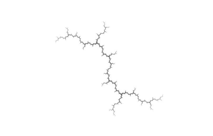
Figure 3: The Julia set of $P(z)=z^{2}+i$.

An important source of trees is given by Julia sets of postcritically-finite polynomials without periodic critical points in $\mathbb{C}$. It follows from DH (84) (or see (CG, 93, Theorem V.4.2)) that the Julia sets of such polynomials are indeed trees. One can show that the Julia set $\mathcal{J}(P)$ of the polynomial $P(z)=z^{2}+i$ (see Figure 3) satisfies the conditions in Theorem 1.1. Accordingly, $\mathcal{J}(P)$ is homeomorphic to the CSST.

There are several directions in which one can pursue these topics further. For example, one can study the topology of more general trees than those in the classes $\mathcal{T}_{m}$. One may want to replace $m$ with any finite (or even infinite) list of allowed valences for branch points, including branch points of infinite valence. In an earlier version of our paper, we discussed this in more detail. Since we learned that these results are already contained in CC (98), we decided to skip this in the present version.

There is one important variant of Theorem 1.2 that we like to mention though. Namely, one can consider the (non-empty) class $\mathcal{T}_{\infty}$ of trees $T$ such that $\nu_{T}(x)\in\{1,2,\infty\}$ for all $x\in T$ and such that the set of branch points of $T$ (i.e., in this case the set $\{x\in T:\nu_{T}(x)=\infty\}$) is dense in $T$. Then all trees in $\mathcal{T}_{\infty}$ are homeomorphic to each other (our method of proof does not directly apply here, but one can use our approach based on a more general version of Proposition 5). Moreover, each tree $T$ in $\mathcal{T}_{\infty}$ is universal in the sense that every tree $S$ admits a topological embedding into $T$. These results are due to Waszewski Wa (23) (see (Na, 92, Section 10.4) for a modern exposition of this universality property; see also Ch (80) for a discussion of a universality property of the trees in $\mathcal{T}_{m}$, $m\in\mathbb{N}$, $m\geq 3$).

Trees in $\mathcal{T}_{\infty}$ are also interesting, because they naturally arise in probabilistic models. More specifically, the so-called stable trees with index $\alpha\in(1,2]$ are generalizations of the CRT (see (LG, 06, Section 4) for the definition). For fixed $\alpha\in(1,2)$, a sample $T$ of such a stable tree belongs to $\mathcal{T}_{\infty}$ almost surely (LG, 06, Proposition 5.2 (ii)). By the previous discussion this implies that two independent samples of stable trees for given $\alpha\in(1,2)$ are almost surely homeomorphic. Note that the Julia set of a polynomial never belongs to $\mathcal{T}_{\infty}$. This follows from results due to Kiwi (see (Kiw, 02, Theorem 1.1)).

Another direction for further investigations are questions that are more related to geometric properties of metric trees, in contrast to purely topological properties. In particular, one can study the quasiconformal geometry of the CSST and other trees (for a survey on the general topic of quasiconformal geometry see Bo (06)).

One of the basic notion here is the concept of quasisymmetric equivalence. By definition two metric spaces $X$ and $Y$ are called quasisymmetrically equivalent if there exists a quasisymmetry $f\colon X\rightarrow Y$. Roughly speaking, a quasisymmetry is a homeomorphism with good geometric control: it sends metric balls to “roundish” sets with uniformly controlled eccentricity (for the precise definition of a quasisymmetry and other basic concepts of quasiconformal geometry see He (01)). Since every quasisymmetry is a homeomorphism, two spaces are homeomorphic if they are quasisymmetrically equivalent. So this gives a stronger type of equivalence for metric spaces that has a more geometric flavor and goes beyond mere topology.

A natural problem in this context is to characterize the CCST $\mathbb{T}$ up to quasisymmetric equivalence, similar to Proposition 3 which gives a topological characterization. This problem is solved in BM19b . The precise statement is too technical to be included here, but roughly speaking the conditions on a metric tree $T$ to be quasisymmetrically equivalent to $\mathbb{T}$ are similar in sprit to the conditions in Proposition 3, but of a more “quantitative” nature.

For example, one of the conditions stipulates that $T$ be trivalent (i.e., all branch points of $T$ are triple points), but not only should the branch points of $T$ form a dense subset of $T$, but $T$ should be uniformly branching in the sense that every arc $\alpha\subseteq T$ contains a branch point $p$ of height $H_{T}(p)$ comparable to the diameter of $\alpha$. Here the height $H_{T}(p)$ is the diameter of the third largest branch of $p$ (see the discussion around (5) for more details).

In our proof of Theorem 1.1 we first realized that this concept of height of a branch point plays a very important role in understanding the geometry and topology of trees. This concept is also used in BM19a ; BM19b .

The present paper and BM19a ; BM19b have another common feature. In all of these works it is important to have good decompositions of the spaces studied, depending on the problem under consideration. This line of thought in the context of quasiconformal geometry can be traced back to (BM, 17, Proposition 18.8). More recently, Kigami Kig (18) has systematically investigated such decompositions in the general framework of partitions of a space given by sets that are labeled by the vertices of a (simplicial) tree. This common philosophy with other recent work is the main motivation why we wanted to present the proof of the known Theorem 1.2 from our perspective.

One can use the characterization of the CSST up to quasisymmetric equivalence established in BM19a to prove the following statement (unpublished work by the authors): if the Julia set $\mathcal{J}(P)$ of a postcritically-finite polynomial $P$ with no periodic critical points in $\mathbb{C}$ is homeomorphic to the CSST, then $\mathcal{J}(P)$ is quasisymmetrically equivalent to the CSST.

Finally, we mention in passing that the geometric properties of the continuum random tree (CRT) were considered in the recent paper LR (19) by Lin and Rohde. Though Lin and Rohde do not study quasisymmetric equivalence, many of their considerations still fit into the general framework of quasiconformal geometry.

The present paper is organized as follows. In Section 2 we state and prove a general criterion for two metric spaces to be homeomorphic based on the existence of combinatorially equivalent decompositions of the spaces. In Section 3 we collect some general facts about trees that we use later. The CSST is studied in Section 4. There we provide proofs of Propositions 1, 2, 3, and 4. In Section 5 we explain how to decompose trees in $\mathcal{T}_{m}$ with $m\in\mathbb{N}$, $m\geq 3$. Based on this, we then present a proof Theorem 1.2. Theorem 1.1 is an immediate consequence.

2 Constructing homeomorphisms between spaces

Throughout this paper, we use fairly standard metric space notation. If $(X,d)$ is a metric space, then we denote by $B(a,r)=\{x\in X\colon d(a,x)<r\}$ the open ball of radius $r>0$ centered at $a\in X$. If $A,B\subseteq X$, then $\operatorname{diam}(A)=\sup\{d(x,y):x,y\in A\}$ is the diameter of $A$ and $\operatorname{dist}(A,B)=\inf\{d(x,y):x\in A,\,y\in B\}$ the (minimal) distance of $A$ and $B$. Similarly, if $a\in X$, then $\operatorname{dist}(a,B)=\operatorname{dist}(\{a\},B)$ denotes the distance of the point $a$ to the set $B$. Finally, if $\gamma$ is a path in $X$, then $\operatorname{length}(\gamma)$ stands for its length.

Before we discuss trees in more detail and turn our attention to the CSST, we will establish the following proposition that is the key to showing that two trees are homeomorphic. The statement will also give us some guidance for the desired properties of tree decompositions that we will discuss in the following sections. The proposition is inspired by (BM, 17, Proposition 18.8), which provided geometric conditions for the decomposition of a space that can be used to construct quasisymmetric homeomorphisms.

Proposition 5

Let $(X,d_{X})$ and $(Y,d_{Y})$ be compact metric spaces. Suppose that for each $n\in\mathbb{N}$, the space $X$ admits a decomposition $X=\bigcup_{i=1}^{M_{n}}X_{n,i}$ as a finite union of non-empty compact subsets $X_{n,i}$, $i=1,\dots,M_{n}\in\mathbb{N}$, with the following properties for all $n$, $i$, and $j$:

• Each set $X_{n+1,j}$ is the subset of some set $X_{n,i}$.

• Each set $X_{n,i}$ is equal to the union of some of the sets $X_{n+1,j}$.

• $\max_{1\leq i\leq M_{n}}\operatorname{diam}(X_{n,i})\to 0$ as $n\to\infty$.

Suppose that for $n\in\mathbb{N}$ the space $Y$ admits a decomposition $Y=\bigcup_{i=1}^{M_{n}}Y_{n,i}$ as a union of non-empty compact subsets $Y_{n,i}$, $i=1,\dots,M_{n}$, with properties analogous to (i)–(iii) such that

$$X_{n+1,j}\subseteq X_{n,i}\mbox{ if and only if }~{}Y_{n+1,j}\subseteq Y_{n,i}$$ (3)

and

$$X_{n,i}\cap X_{n,j}\neq\emptyset\mbox{ if and only if }~{}Y_{n,i}\cap Y_{n,j}\neq\emptyset$$ (4)

for all $n$, $i$, $j$.

Then there exists a unique homeomorphism $f\colon X\rightarrow Y$ such that $f(X_{n,i})=Y_{n,i}$ for all $n$ and $i$.

In particular, under these assumptions the spaces $X$ and $Y$ are homeomorphic.

Proof

We define a map $f\colon X\rightarrow Y$ as follows. For each point $x\in X$, by (ii) and (iii) there exists a nested sequence of sets $X_{n,i_{n}}$, $n\in\mathbb{N}$, such that $\{x\}=\bigcap_{n}X_{n,i_{n}}.$ Then the corresponding sets $Y_{n,i_{n}}$, $n\in\mathbb{N}$, are also nested by (3). Since these sets are non-empty and compact, by condition (iii) for the space $Y$ this implies that there exists a unique point $y\in\bigcap_{n}Y_{n,i_{n}}$. We define $f(x)=y$.

Then $f$ is well-defined. To see this, suppose we have another nested sequence $X_{n,i^{\prime}_{n}}$, $n\in\mathbb{N}$, such that $\{x\}=\bigcap_{n}X_{n,i_{n}^{\prime}}.$ Then there exists a unique point $y^{\prime}\in\bigcap_{n}Y_{n,i^{\prime}_{n}}$. Now $x\in X_{n,i_{n}}\cap X_{n,i^{\prime}_{n}}$ and so $Y_{n,i_{n}}\cap Y_{n,i^{\prime}_{n}}\neq\emptyset$ for all $n\in\mathbb{N}$ by (4). By condition (iii) for $Y$, this is only possible if $y=y^{\prime}$. So $f\colon X\rightarrow Y$ is indeed well-defined.

One can define a map $g\colon Y\rightarrow X$ by a similar procedure. Namely, for each $y\in Y$ we can find a nested sequence $Y_{n,i_{n}}$, $n\in\mathbb{N}$, such that $\{y\}=\bigcap_{n}Y_{n,i_{n}}.$ Then there exists a unique point $x\in\bigcap_{n}X_{n,i_{n}}$ and if we set $g(y)=x$, we obtain a well-defined map $g\colon Y\rightarrow X$.

It is obvious from the definitions that the maps $f$ and $g$ are inverse to each other. Hence they define bijections between $X$ and $Y$.

Conditions (i) and (ii) imply that if $X_{k,i}$ is a set in one of the decompositions of $X$ and $x\in X_{k,i}$, then there exists a nested sequence $X_{n,i_{n}}$, $n\in\mathbb{N}$, with $X_{k,i_{k}}=X_{k,i}$ and $\{x\}=\bigcap_{n}X_{n,i_{n}}.$ This implies that $f(x)\in Y_{k,i}$ and so $f(X_{k,i})\subseteq Y_{k,i}$. Similarly, $g(Y_{k,i})\subseteq X_{k,i}$. Since $g=f^{-1}$, we have $f(X_{k,i})=Y_{k,i}$ as desired. It is clear that this last condition together with our assumptions determines $f$ uniquely.

It remains to show that $f$ is a homeomorphism. For this it suffices to prove that $f$ and $f^{-1}=g$ are continuous. Since the roles of $f$ and $g$ are completely symmetric, it is enough to establish that $f$ is continuous.

For this, let $\epsilon>0$ be arbitrary. By (iii) we can choose $n\in\mathbb{N}$ such that

$$\max\{\operatorname{diam}(Y_{n,i}):1\leq i\leq M_{n}\}<\epsilon/2.$$

Since the sets $X_{n,i}$ are compact, there exists $\delta>0$ such that

$$\operatorname{dist}(X_{n,i},X_{n,j})>\delta,$$

whenever $i,j\in\{1,\dots,M_{n}\}$ and $X_{n,i}\cap X_{n,j}=\emptyset$.

Now suppose that $a,b\in X$ are arbitrary points with $d_{X}(a,b)<\delta$. We claim that then $d_{Y}(f(a),f(b))<\epsilon$. Indeed, we can find $i,j\in\{1,\dots,M_{n}\}$ such that $a\in X_{n,i}$ and $b\in X_{n,j}$. Since $d_{X}(a,b)<\delta$, we then necessarily have $X_{n,i}\cap X_{m,j}\neq\emptyset$ by definition of $\delta$. So $Y_{n,i}\cap Y_{n,j}\neq\emptyset$ by (4). Moreover, $f(a)\in f(X_{n,i})=Y_{n,i}$ and $f(b)\in f(X_{n,j})=Y_{n,j}$. Hence

$$d_{Y}(f(a),f(b))\leq\operatorname{diam}(Y_{n,i})+\operatorname{diam}(Y_{n,j})<\epsilon.$$

The continuity of $f$ follows. ∎

3 Topology of trees

In this section we fix some terminology and collect some general facts about trees. We do not claim any originality of this material. All of it is standard and well-known, but we did not try to track it down in the literature. Our objective is to make our presentation self-contained, and to have convenient reference points for future work. For general background on trees or dendrites we refer to (Wh, 63, Chapter V), (Ku, 68, Section §51 VI), (Na, 92, Chapter X)), and the literature mentioned there.

An arc $\alpha$ in a metric space is a homeomorphic image of the unit interval $[0,1]\subseteq\mathbb{R}$. The points corresponding to $0$ and $1$ are called the endpoints of $\alpha$.

Let $T$ be a tree. Then the last part of Definition 2 is equivalent to the requirement that for all points $a,b\in T$ with $a\neq b$, there exists a unique arc in $T$ joining $a$ and $b$, i.e., it has the endpoints $a$ and $b$. We use the notation $[a,b]$ for this unique arc. It is convenient to allow $a=b$ here. Then $[a,b]$ denotes the degenerate arc consisting only of the point $a=b$. Sometimes we want to remove one or both endpoints from the arc $[a,b]$. Accordingly, we define $(a,b)=[a,b]\backslash\{a,b\}$, $[a,b)=[a,b]\backslash\{b\}$ and $(a,b]=[a,b]\backslash\{a\}$. In Section 4 we will not use this notation for arcs in a tree. There $[a,b]$ will always denote the Euclidean line segment joining two points $a,b\in\mathbb{C}$.

A metric space $X$ is called path-connected if any two points $a,b\in X$ can be joined by a path in $X$, i.e., there exists a continuous map $\gamma\colon[0,1]\rightarrow X$ such that $\gamma(0)=a$ and $\gamma(1)=b$. The space $X$ is arc-connected if any two distinct points in $X$ can be joined by an arc in $X$. The image of a path joining two distinct points in a metric space always contains an arc joining these points (this follows from the fact that every Peano space is arc-connected; see (HY, 61, Theorem 3.15, p. 116)). In particular, every path-connected metric space is arc-connected.

Lemma 1

Let $(T,d)$ be a tree. Then for each $\epsilon>0$ there exists $\delta>0$ such that for all $a,b\in T$ with $d(a,b)<\delta$ we have $\operatorname{diam}([a,b])<\epsilon$.

Proof

Fix $\epsilon>0$. Since $T$ is a compact, connected, and locally connected metric space, it is a Peano space. So by the Hahn-Mazurkiewicz theorem there exists a continuous surjective map $\varphi\colon[0,1]\rightarrow T$ of the unit interval onto $T$ (HY, 61, Theorem 3.30, p. 129). By uniform continuity of $\varphi$ we can represent $[0,1]$ as a union $[0,1]=I_{1}\cup\dots\cup I_{n}$ of finitely many closed intervals $I_{1},\dots,I_{n}\subseteq[0,1]$ with $\operatorname{diam}(X_{k})<\epsilon/2$, where $X_{k}=\varphi(I_{k})$ for $k=1,\dots,n$. The sets $X_{k}=\varphi(I_{k})$ are compact. This implies that there exists $\delta>0$ such that $\operatorname{dist}(X_{i},X_{j})>\delta$, whenever $i,j\in\{1,\dots,n\}$ and $X_{i}\cap X_{j}=\emptyset$.

Now let $a,b\in T$ with $d(a,b)<\delta$ be arbitrary. We may assume $a\neq b$. Then there exist $i,j\in\{1,\dots,n\}$ with $a\in X\coloneqq X_{i}$ and $b\in Y\coloneqq X_{j}$. By choice of $\delta$ we must have $X\cap Y\neq\emptyset$. As continuous images of intervals, the sets $X$ and $Y$ are path-connected. Since $X\cap Y\neq\emptyset$, the union $X\cup Y$ that contains the points $a$ and $b$ is also path-connected. This implies that $X\cup Y$ is arc-connected, and so there exists an arc $\alpha\subseteq X\cup Y$ with endpoints $a$ and $b$. The unique such arc in the tree $T$ is $[a,b]$, and so $[a,b]=\alpha\subseteq X\cup Y$. This implies

$$\operatorname{diam}([a,b])\leq\operatorname{diam}(X)+\operatorname{diam}(Y)<\epsilon,$$

as desired. ∎

Lemma 2

Let $(T,d)$ be a tree and $p\in T$. Then the following statements are true:

• Each component $U$ of $T\backslash\{p\}$ is an open and arc-connected subset of $T$.

• If $U$ is a component of $T\backslash\{p\}$, then $\overline{U}=U\cup\{p\}$ and $\partial U=\{p\}$.

• Two points $a,b\in T\backslash\{p\}$ lie in the same component of $T\backslash\{p\}$ if and only if $p\not\in[a,b]$.

Proof

(i) The set $T\backslash\{p\}$ is open. Since $T$ is locally connected, each component $U$ of $T\backslash\{p\}$ is also open.

For $a,b\in U$ we write $a\sim b$ if $a$ and $b$ can be joined by a path in $U$. Obviously, this defines an equivalence relation on $U$. The equivalence classes are open subsets of $T$. To see this, suppose $a,b\in U$ can be joined by a path $\beta$ in $U$. Then for all points $x$ in a sufficiently small neighborhood $V\subseteq U$ of $b$ we have $[b,x]\subseteq U$ as follows from Lemma 1. So by concatenating $\beta$ with (a parametrization of) the arc $[b,x]$, we obtain a path $\beta^{\prime}$ in $U$ that joins $a$ and $x\in V$. This shows that every point $b$ in the equivalence class of $a$ has a neighborhood $V$ that also belongs to this equivalence class.

We see that the equivalence classes of $\sim$ partition $U$ into open sets. Since $U$ is connected, there can only be one such set. It follows that $U$ is path-connected and hence also arc-connected.

(ii) Let $U$ be a (non-empty) component of $T\backslash\{p\}$. We choose a point $a\in U$. The set $[a,p)$ is connected, contained in $T\backslash\{p\}$, and meets $U$ in $a$. Hence $[a,p)\subseteq U$. This implies that $p\in\overline{U}$. On the other hand, the set $U\cup\{p\}$ is closed, because its complement is a union of components of $T\backslash\{p\}$ and hence open by (i). Thus $\overline{U}=U\cup\{p\}$. By (i) no point in $U$ is a boundary point of $U$, and so $\partial U=\{p\}$.

(iii) If $a,b\in T\backslash\{p\}$ and $p\not\in[a,b]$, then $[a,b]$ is a connected subset of $T\backslash\{p\}$. Hence $[a,b]$ lies in a component $U$ of $T\backslash\{p\}$. In particular, $a,b\in[a,b]$ lie in the same component $U$ of $T\backslash\{p\}$.

Conversely, suppose that $a,b\in T\backslash\{p\}$ lie in the same component $U$ of $T\backslash\{p\}$. We know by (i) that $U$ is arc-connected. Hence there exists a (possibly degenerate) arc $\alpha\subseteq U$ with endpoints $a$ and $b$. But the unique such arc in $T$ is $[a,b]$. Hence $[a,b]=\alpha\subseteq U\subseteq T\backslash\{p\}$, and so $p\not\in[a,b]$. ∎

A subset $S$ of a tree $(T,d)$ is called a subtree of $T$ if $S$ equipped with the restriction of the metric $d$ is also a tree as in Definition 2. Every subtree $S$ of $T$ contains two points and hence a non-degenerate arc. In particular, every subtree $S$ of $T$ is an infinite, actually uncountable set.

The following statement characterizes subtrees.

Lemma 3

Let $(T,d)$ be a tree. Then a set $S\subseteq T$ is a subtree of $T$ if and only if $S$ contains at least two points and is closed and connected.

Proof

If $S$ is a subtree of $T$, then $S$ contains at least two points, and is connected and compact. Hence it is a closed subset of $T$. Conversely, suppose that $S$ contains at least two points and is closed and connected. Then $S$ is compact, because $T$ is compact.

Suppose that $a,b\in S$, $a\neq b$, are two distinct points in $S$. We consider the arc $[a,b]\subseteq T$. Suppose there exists a point $p\in[a,b]$ with $p\not\in S$. Then $p\neq a,b$, and so by Lemma 2 (iii), the points $a$ and $b$ lie in different components of $T\backslash\{p\}$. This is impossible, because the connected set $S\subseteq T\backslash\{p\}$ must be contained in exactly one component of $T\backslash\{p\}$. This shows that $[a,b]\subseteq S$ and so the points $a$ and $b$ can be joined by an arc in $S$. This arc in $S$ is unique, because it is unique in $T$.

It remains to show that $S$ is locally connected, i.e., every point in $S$ has arbitrarily small connected relative neighborhoods. To see this, let $a\in S$ and $\epsilon>0$ be arbitrary. Then by Lemma 1 we can find $\delta>0$ such that $[a,x]\subseteq B(a,\epsilon)$ whenever $x\in B(a,\delta)$. Now let $M$ be the union of all arcs $[a,x]$ with $x\in S\cap B(a,\delta)$. These arcs lie in $S$ and so $M$ is a connected set contained in $S\cap B(a,\epsilon)$. Moreover, $S\cap B(a,\delta)\subseteq M$ and so $M$ is a connected relative (not necessarily open) neighborhood of $a$ in $S$. This shows that $S$ is locally connected. We conclude that $S$ is indeed a subtree of $T$. ∎

Lemma 4

Let $(T,d)$ be a tree, $p\in T$, and $U$ a component of $T\backslash\{p\}$. Then $B=U\cup\{p\}$ is a subtree of $T$ and $p$ is a leaf of $B$.

Proof

It follows from Lemma 2 (i) and (ii) that the set $U$ is connected and that $B=U\cup\{p\}=\overline{U}$. This implies that $B$ is closed and connected. Since $U\neq\emptyset$ and $p\not\in U$, the set $B$ contains at least two points. Hence $B$ is a subtree of $T$ by Lemma 3. Since $B\backslash\{p\}=U$ is connected, $p$ is a leaf of $B$. ∎

If the subtree $B=U\cup\{p\}$ is as in the previous lemma, then we call $B$ a branch of $p$ in $T$ (or just a branch of $p$ if $T$ is understood).

Lemma 5

Let $(T,d)$ be a tree, $S\subseteq T$ be a subtree of $T$, and $p\in S$. Then every branch $B^{\prime}$ of $p$ in $S$ is contained in a unique branch $B$ of $p$ in $T$. The assignment $B^{\prime}\mapsto B$ is an injective map between the sets of branches of $p$ in $S$ and in $T$. If $p$ is an interior point of $S$, then this map is a bijection.

In particular, if under the given assumptions $\nu_{T}(p)$ is the valence of $p$ in $T$ and $\nu_{S}(p)$ the valence of $p$ in $S$, then $\nu_{S}(p)\leq\nu_{T}(p)$. Here we have equality if $p$ is an interior point of $S$.

If $p\in S$ is a leaf of $T$, then $T$ has only one branch $B$ at $p$, namely $B=T$. Hence $1\leq\nu_{S}(p)\leq\nu_{T}(p)\leq 1$, and so $\nu_{S}(p)=1$. This means that $p$ is also a leaf of $S$. More informally, we can say that the property of a point being a leaf in $T$ is passed to subtrees that contain the point.

Proof

If $B^{\prime}$ is a branch of $p$ in $S$, then $B^{\prime}=U^{\prime}\cup\{p\}$, where $U^{\prime}$ is a component of $S\backslash\{p\}$. Then $U^{\prime}$ is a connected subset of $T\backslash\{p\}$ and so contained in a unique component $U$ of $T\backslash\{p\}$. Then $B=U\ \cup\{p\}$ is a branch of $p$ in $T$ with $B^{\prime}\subseteq B$ and it is clear that $B$ is the unique such branch.

To show injectivity of the map $B^{\prime}\mapsto B$, let $B_{1}^{\prime}$ and $B_{2}^{\prime}$ be two distinct branches of $p$ in $S$. Pick points $a\in B_{1}^{\prime}\backslash\{p\}$ and $b\in B_{2}^{\prime}\backslash\{p\}$. Then $a$ and $b$ lie in different components of $S\backslash\{p\}$ and so $p\in[a,b]$ by Lemma 2 (iii) applied to the tree $S$. Hence $a$ and $b$ lie in different components of $T\backslash\{p\}$, and so in different branches of $p$ in $T$. This implies that $B_{1}^{\prime}$ and $B_{2}^{\prime}$ must be contained in different branches of $p$ in $T$. This shows that the map $B^{\prime}\mapsto B$ is indeed injective.

Now assume in addition that $p$ is an interior point of $S$. To show surjectivity of the map $B^{\prime}\mapsto B$, we consider a branch $B$ of $p$ in $T$. Pick a point $a\in B\backslash\{p\}$. Then $[a,p)\subseteq B\backslash\{p\}$, because $B$ is a subtree of $T$. Since $p$ is an interior point of $S$, there exists a point $x\in[a,p)$ close enough to $p$ such that $x\in S\backslash\{p\}$. If $B^{\prime}$ is the unique branch of $p$ in $S$ that contains $x$, then we have $x\in B^{\prime}\cap B$. This implies $B^{\prime}\subseteq B$. Hence the map $B^{\prime}\mapsto B$ is also surjective, and so a bijection. ∎

Lemma 6

Let $(T,d)$ be a tree, $p,a_{1},a_{2},a_{3}\in T$ with $p\neq a_{1},a_{2},a_{3}$ and suppose that the sets $[a_{1},p)$, $[a_{2},p)$, $[a_{3},p)$ are pairwise disjoint. Then the points $a_{1},a_{2},a_{3}$ lie in different components of $T\backslash\{p\}$ and $p$ is a branch point of $T$.

Proof

The arcs $[a_{1},p]$ and $[a_{2},p]=[p,a_{2}]$ have only the point $p$ in common. So their union $[a_{1},p]\cup[p,a_{2}]$ is an arc and this arc must be equal to $[a_{1},a_{2}]$. Hence $p\in[a_{1},a_{2}]$ which by Lemma 2 (iii) implies that $a_{1}$ and $a_{2}$ lie in different components of $T\backslash\{p\}$. A similar argument shows that $a_{3}$ must be contained in a component of $T\backslash\{p\}$ different from the components containing $a_{1}$ and $a_{2}$. In particular, $T\backslash\{p\}$ has at least three components and so $p$ is a branch point of $T$. The statement follows. ∎

Lemma 7

Let $(T,d)$ be a tree such that the branch points of $T$ are dense in $T$. If $a,b\in T$ with $a\neq b$, then there exists a branch point $c\in(a,b)$.

Proof

We pick a point $x_{0}\in(a,b)\neq\emptyset$. Then $x_{0}$ has positive distance to both $a$ and $b$. This and Lemma 1 imply that we can find $\delta>0$ such that for all $x\in B(x_{0},\delta)$ the arc $[x,x_{0}]$ has uniformly small diameter and so does not contain $a$ or $b$.

Since branch points are dense in $T$, we can find a branch point $p\in B(x_{0},\delta)$. Then $a,b\not\in[p,x_{0}]$. If $p\in(a,b)$, we are done.

In the other case, we have $p\not\in(a,b)$. If we travel from $p$ to $x_{0}\in(a,b)$ along $[p,x_{0}]$, we meet $[a,b]$ in a first point $c\in(a,b)$. Then $a,b,p\neq c$. Moreover, the sets $[a,c)$, $[b,c)$, $[p,c)$ are pairwise disjoint. Hence $c\in(a,b)$ is a branch point of $T$ as follows from Lemma 6. ∎

Lemma 8

Let $(X,d)$ be a compact, connected, and locally connected metric space, $J$ an index set, $p_{i}\in T$, and $U_{i}$ a component of $X\backslash\{p_{i}\}$ for each $i\in J$. Suppose that

$$U_{i}\cap U_{j}=\emptyset$$

for all $i,j\in J$, $i\neq j$. Then $J$ is a countable set. If there exists $\delta>0$ such that $\operatorname{diam}(U_{i})>\delta$ for each $i\in J$, then $J$ is finite.

Informally, the space $X$ cannot contain a “comb” with too many long teeth.

Proof

We prove the last statement first. We argue by contradiction and assume that $\operatorname{diam}(U_{i})>\delta>0$ for each $i\in J$, where $J$ is an infinite index set. Then we can choose a point $x_{i}\in U_{i}$ such that $d(x_{i},p_{i})\geq\delta/2$. The set $A=\{x_{i}:i\in J\}$ is infinite and so it must have a limit point $q\in X$, because $X$ is compact. Since $X$ is locally connected, there exists a connected neighborhood $N$ of $q$ such that $N\subseteq B(q,\delta/8)$. Since $q$ is a limit point of $A$, the set $N$ contains infinitely many points in $A$. In particular, we can find $i,j\in J$ with $x_{i},x_{j}\in N$ and $i\neq j$. Then

$$\operatorname{dist}(p_{i},N)\geq d(p_{i},x_{i})-\operatorname{diam}(N)\geq\delta/2-\delta/4>0,$$

and so $N\subseteq X\backslash\{p_{i}\}$. Since the connected set $N$ meets $U_{i}$ in the point $x_{i}$, this implies that $N\subseteq U_{i}$. Similarly, $N\subseteq U_{j}$. This is impossible, because we have $i\neq j$ and so $U_{i}\cap U_{j}\neq\emptyset$, while $\emptyset\neq N\subseteq U_{i}\cap U_{j}$.

To prove the first statement, note that $\operatorname{diam}(U_{i})>0$ for each $i\in J$. Indeed, otherwise $\operatorname{diam}(U_{i})=0$ for some $i\in J$. Then $U_{i}$ consists of only one point $a$. Since $X$ is locally connected, the component $U_{i}$ of $X\backslash\{p_{i}\}$ is an open set. So $a$ is an isolated point of $X$. This is impossible, because the metric space $X$ is connected and so it does not have isolated points.

Now we write $J=\bigcup_{n\in\mathbb{N}}J_{n}$, where $J_{n}$ consists of all $i\in J$ such that $\operatorname{diam}(U_{i})>1/n$. Then each set $J_{n}$ is finite by the first part of the proof. This implies that $J$ is countable. ∎

We can apply the previous lemma to a tree $T$ and choose for each $p_{i}$ a fixed branch point $p$ of $T$. Then it follows that $p$ can have at most countably many distinct complementary components $U_{i}$ and hence there are only countably many distinct branches $B_{i}=U_{i}\cup\{p\}$ of $p$. Moreover, since $\operatorname{diam}(B_{i})=\operatorname{diam}(\overline{U}_{i})=\operatorname{diam}(U_{i})$, there can only be finitely many of these branches whose diameter exceeds a given positive number $\delta>0$. In particular, we can label the branches of $p$ by numbers $n=1,2,3,\dots$ so that

$$\operatorname{diam}(B_{1})\geq\operatorname{diam}(B_{2})\geq\operatorname{diam}(B_{3})\geq\dots\,.$$

We now set

$$H_{T}(p)=\operatorname{diam}(B_{3})$$ (5)

and call $H_{T}(p)$ the height of the branch point $p$ in $T$. So the height of a branch point $p$ is the diameter of the third largest branch of $p$.

Lemma 9

Let $(T,d)$ be a tree and $\delta>0$. Then there are at most finitely many branch points $p\in T$ with height $H_{T}(p)>\delta$.

Proof

We argue by contradiction and assume that this is not true. Then the set $E$ of branch points $p$ in $T$ with $H_{T}(p)>\delta$ has infinitely many elements. Since $T$ is compact, the set $E$ has a limit point $q\in T$.

Claim. There exists a branch $Q$ of $q$ such that the set $E\cap Q$ is infinite and has $q$ as a limit point.

Otherwise, $q$ has infinitely many distinct branches $Q_{n}$, $n\in\mathbb{N}$, that contain a point $a_{n}\in E\cap(Q_{n}\backslash\{q\})$. Then $a_{n}$ is a branch point with $H_{T}(a_{n})>\delta$ which implies that $a_{n}$ has at least three branches whose diameters exceed $\delta$. At least one of them does not contain $q$. If we denote such a branch of $a_{n}$ by $V_{n}$, then $V_{n}$ is a connected subset of $T\backslash\{q\}$. It meets $Q_{n}\backslash\{q\}$, because $a_{n}\in(Q_{n}\backslash\{q\})\cap V_{n}$. It follows that $V_{n}\subseteq Q_{n}$ and so $\operatorname{diam}(Q_{n})\geq\operatorname{diam}(V_{n})>\delta$. Since the branches $Q_{n}$ of $q$ are all distinct for $n\in\mathbb{N}$, this contradicts Lemma 8 (see the discussion after the proof of this lemma). The Claim follows.

We fix a branch $Q$ of $q$ as in the Claim. For each $n\in\mathbb{N}$ we will now inductively construct branch points $p_{n}\in E\cap(Q\backslash\{q\})$ together with a branch $B_{n}$ of $p_{n}$ and an auxiliary compact set $K_{n}\subseteq T$. They will satisfy the following conditions for each $n\in\mathbb{N}$:

• $\operatorname{diam}(B_{n})>\delta$,

• the sets $B_{1},\dots,B_{n}$ are disjoint,

• the set $K_{n}$ is compact and connected, and

  $$B_{1}\cup\dots\cup B_{n}\subseteq K_{n}\subseteq Q\backslash\{q\}.$$

We pick an arbitrary branch point $p_{1}\in E\cap(Q\backslash\{q\})$ to start. Then we can choose a branch $B_{1}$ of $p_{1}$ that does not contain $q$ and satisfies $\operatorname{diam}(B_{1})>\delta$. We set $K_{1}=B_{1}$. Then $K_{1}$ is a compact and connected set that does not contain $q$ and meets $Q$, because $p_{1}\in K_{1}\cap Q$. Hence $K_{1}\subseteq Q\backslash\{q\}$.

Suppose for some $n\in\mathbb{N}$, a branch point $p_{k}\in E\cap Q$, a branch $B_{k}$ of $p_{k}$, and a set $K_{k}$ with the properties (i)–(iii) have been chosen for all $1\leq k\leq n$.

Since $q\not\in K_{n}$, we have $\operatorname{dist}(q,K_{n})>0$, and so we can find a branch point $p_{n+1}\in E\cap(Q\backslash\{p\})$ sufficiently close to $q$ such that $p_{n+1}\not\in K_{n}$. This is possible, because $q$ is a limit point of $E\cap(Q\backslash\{q\})$. Since the set $K_{n}\subseteq T\backslash\{p_{n+1}\}$ is connected, it must be contained in a branch of $p_{n+1}$. Since there are three branches of $p_{n+1}\neq q$ whose diameters exceed $\delta$, we can pick one of them that contains neither $q$ nor $K_{n}$. Let $B_{n+1}$ be such a branch of $p_{n+1}$. Then $\operatorname{diam}(B_{n+1})>\delta$ and so (i) is true for $n+1$. We have $B_{n+1}\cap K_{n}=\emptyset$; so (iii) shows that $B_{n+1}$ is disjoint from the previously chosen disjoint sets $B_{1},\dots,B_{n}$. This gives (ii).

Since $p_{n},p_{n+1}\in Q\backslash\{q\}$, the arc $[p_{n},p_{n+1}]$ does not contain $q$ (see Lemma 2 (iii)). We also have $p_{n}\in B_{n}\subseteq K_{n}$ and $p_{n+1}\in B_{n+1}$, which implies that the set $K_{n+1}\coloneqq K_{n}\cup[p_{n},p_{n+1}]\cup B_{n+1}\subseteq Q\backslash\{q\}$ is compact and connected. We have

$$B_{1}\cup\dots\cup B_{n}\cup B_{n+1}\subseteq K_{n}\cup B_{n+1}\subseteq K_{n+1}\subseteq Q\backslash\{q\},$$

and so $K_{n+1}$ has property (iii).

Continuing with this process, we obtain disjoint branches $B_{n}$ for all $n\in\mathbb{N}$ that satisfy (i). The last part of Lemma 8 implies that this is impossible and we get a contradiction. ∎

4 Basic properties of the continuum self-similar tree

We now we study the properties of the continuum self-similar tree (CSST). Unless otherwise specified, all metric notions in this section refer to the Euclidean metric on the complex plane $\mathbb{C}$. In this section, $i$ always denotes the imaginary unit and we do not use this letter for indexing as in the other sections. If $a,b\in\mathbb{C}$ we denote by $[a,b]$ the Euclidean line segment in $\mathbb{C}$ joining $a$ and $b$. We also use the usual notation for open or half-open line segments. So $[a,b)=[a,b]\backslash\{b\}$, etc.

For the proof of Proposition 1 we consider a coding procedure of certain points in the complex plane by words in an alphabet. We first fix some terminology related to this. We consider a non-empty set $\mathcal{A}$. Then we call $\mathcal{A}$ an alphabet and refer to the elements in $\mathcal{A}$ as the letters in this alphabet. In this paper we will only use alphabets of the form $\mathcal{A}=\{1,2,\dots,m\}$ with $m\in\mathbb{N}$, $m\geq 3$. We consider the set $W(\mathcal{A})\coloneqq\mathcal{A}^{\mathbb{N}}$ of infinite sequences in $\mathcal{A}$ as the set of infinite words in the alphabet $\mathcal{A}$ and write the elements $w\in W(\mathcal{A})$ in the form $w=w_{1}w_{2}\ldots$, where it is understood that $w_{k}\in\mathcal{A}$ for $k\in\mathbb{N}$. Similarly, we set $W_{n}(\mathcal{A})\coloneqq\mathcal{A}^{n}$ and consider $W_{n}(\mathcal{A})$ as the set of all words in the alphabet $\mathcal{A}$ of length $n$. We write the elements $w\in W_{n}(\mathcal{A})$ in the form $w=w_{1}\dots w_{n}$ with $w_{k}\in\mathcal{A}$ for $k=1,\dots,n$. We use the convention that $W_{0}(\mathcal{A})=\{\emptyset\}$ and consider the only element $\emptyset$ in $W_{0}(\mathcal{A})$ as the empty word of length $0$. Finally,

$$W_{*}(\mathcal{A})\coloneqq\bigcup_{n\in\mathbb{N}_{0}}W_{n}(\mathcal{A})$$

is the set of all words of finite length. If $u=u_{1}\dots u_{n}$ is a finite word and $v=v_{1}v_{2}\dots$ is a finite or infinite word in the alphabet $\mathcal{A}$, then we denote by $uv=u_{1}\dots u_{n}v_{1}v_{2}\dots$ the word obtained by concatenating $u$ and $v$. We call $u$ an initial segment and $v$ a tail of the word $w=uv$. If the alphabet $\mathcal{A}$ is understood, then we will simply drop $\mathcal{A}$ from the notation. So $W$ will denote the set of infinite words in $\mathcal{A}$, etc.

For the rest of this section, we use the alphabet $\mathcal{A}=\{1,2,3\}$. So when we write $W$, $W_{n}$, $W_{*}$ it is understood that $\mathcal{A}=\{1,2,3\}$ is the underlying alphabet. There exists a unique metric $d$ on $W=\{1,2,3\}^{\mathbb{N}}$ with the following property. If we have two words $u=u_{1}u_{2}\ldots$ and $v=v_{1}v_{2}\ldots$ in $W$ and $u\neq v$, then for some $n\in\mathbb{N}_{0}$ we have $u_{1}=v_{1}$, …, $u_{n}=v_{n}$, and $u_{n+1}\neq v_{n+1}$. Then $d(u,v)=1/2^{n}$. More informally, two elements $u,v\in W$ are close in this metric precisely if they share a large number of initial letters. The metric space $(W,d)$ is compact and homeomorphic to a Cantor set.

If $n\in\mathbb{N}_{0}$ and $w=w_{1}w_{2}\dots w_{n}\in W_{n}$, we define

$$f_{w}\coloneqq f_{w_{1}}\circ f_{w_{2}}\circ\cdots\circ f_{w_{n}},$$

where we use the maps in (1) in the composition. By convention, $f_{\emptyset}=\text{id}_{\mathbb{C}}$ is the identity map on $\mathbb{C}$. Note that $f_{w}$ is a Euclidean similarity on $\mathbb{C}$ that scales Euclidean distances by the factor $2^{-n}$. If $a,b\in\mathbb{C}$, then $f_{w}([a,b])=[f_{w}(a),f_{w}(b)]$. We will use this repeatedly in the following.

Throughout this section we denote by $H\subseteq\mathbb{C}$ the (closed) convex hull of the four points $1$, $i$, $-1$, and $\tfrac{1}{2}-\frac{i}{2}$ (see Figure 4). We set $H_{k}=f_{k}(H)$ for $k=1,2,3$. Then

$$H_{1}\cup H_{2}\cup H_{3}=f_{1}(H)\cup f_{2}(H)\cup f_{3}(H)\subseteq H.$$

This implies that

$$f_{w}(H)\subseteq H$$ (6)

for all $w\in W_{\ast}$.

\begin{overpic}[scale={0.7}]{Hsets.png} \put(50.0,65.0){ $i$} \put(14.0,25.0){ $-1$} \put(85.0,25.0){ $1$} \put(85.0,25.0){ $1$} \put(70.0,10.0){ $-\frac{1}{2}+\frac{i}{2}$} \put(50.0,25.0){ $0$} \put(30.0,35.0){ $H_{1}$} \put(70.0,20.0){ $H_{2}$} \put(55.0,50.0){ $H_{3}$} \put(40.0,25.0){ $I_{1}$} \put(60.0,25.0){ $I_{2}$} \put(53.0,37.0){ $I_{3}$} \put(75.0,30.0){ $I$} \put(35.0,15.0){ $H$} \end{overpic}

Figure 4: Ilustration of some associated sets.

Lemma 10

There exists a well-defined continuous map $\pi\colon W\rightarrow\mathbb{C}$ given by

$$\pi(w)=\lim_{n\to\infty}f_{w_{1}w_{2}\dots w_{n}}(z_{0})$$

for $w=w_{1}w_{2}\ldots\in W$ and $z_{0}\in\mathbb{C}$. Here the limit exists and is independent of the choice of $z_{0}\in\mathbb{C}$.

The existence of such a map $\pi$ is standard in similar contexts (see, for example, (Hu, 81, Section 3.1, pp. 426–427)). In the following, $\pi\colon W\rightarrow\mathbb{C}$ will always denote the map provided by this lemma.

Proof

Fix $z_{0}\in\mathbb{C}$. Then there exists a constant $C\geq 0$ such that

$$|z_{0}-f_{k}(z_{0})|\leq C$$

for $k=1,2,3$. If $n\in\mathbb{N}_{0}$ and $u\in W_{n}$, then

$$|f_{u}(a)-f_{u}(b)|=\frac{1}{2^{n}}|a-b|$$

for all $a,b\in\mathbb{C}$. This implies that if $w=w_{1}w_{2}\ldots\in W$, $n\in\mathbb{N}$, and $u\coloneqq w_{1}w_{2}\dots w_{n}\in W_{n}$, then

$$|f_{w_{1}w_{2}\dots w_{n}}(z_{0})-f_{w_{1}w_{2}\dots w_{n+1}}(z_{0})| =|f_{u}(z_{0})-f_{u}(f_{w_{n+1}}(z_{0}))|$$

$$=\frac{1}{2^{n}}|z_{0}-f_{w_{n+1}}(z_{0})|\leq\frac{C}{2^{n}}.$$

It follows that $\{f_{w_{1}w_{2}\dots w_{n}}(z_{0})\}_{n\in\mathbb{N}}$ is a Cauchy sequence in $\mathbb{C}$. Hence this sequence converges and

$$\pi(w)=\lim_{n\to\infty}f_{w_{1}w_{2}\dots w_{n}}(z_{0})$$

is well-defined for each $w=w_{1}w_{2}\ldots\in W$.

The limit does not depend on the choice of $z_{0}$. Indeed, if $z^{\prime}_{0}\in\mathbb{C}$ is another point, then

$$|f_{w_{1}w_{2}\dots w_{n}}(z_{0})-f_{w_{1}w_{2}\dots w_{n}}(z^{\prime}_{0})|=\frac{1}{2^{n}}|z_{0}-z^{\prime}_{0}|,$$

which implies that

$$\lim_{n\to\infty}f_{w_{1}w_{2}\dots w_{n}}(z_{0})=\lim_{n\to\infty}f_{w_{1}w_{2}\dots w_{n}}(z^{\prime}_{0}).$$

The definition of $\pi$ shows that if $w=w_{1}w_{2}\ldots\in W$ and $n\in\mathbb{N}_{0}$, then

$$\pi(w)=\pi(w_{1}w_{2}\ldots)=f_{w_{1}\dots w_{n}}(\pi(w_{n+1}w_{n+2}\ldots)).$$ (7)

If we pick $z_{0}\in H$, then (6) and the definition of $\pi$ imply that $\pi(W)\subseteq H$. If we combine this with (7), then we see that if two words $u,v\in W$ start with the same letters $w_{1},\dots,w_{n}$, then

$$|\pi(u)-\pi(v)|\leq\operatorname{diam}(f_{w_{1}\dots w_{n}}(H))=\frac{1}{2^{n}}\operatorname{diam}(H).$$

The continuity of the map $\pi$ follows from this and the definition of the metric $d$ on $W$. ∎

We can now establish the result that is the basis of the definition of the CSST. Again arguments along these lines are completely standard.

Proof of Proposition 1. Let $\pi\colon W\rightarrow\mathbb{C}$ be the map provided by Lemma 10 and define $\mathbb{T}=\pi(W)\subseteq\mathbb{C}$. Since $W$ is compact and $\pi$ is continuous, the set $\mathbb{T}$ is non-empty and compact. The relation (2) immediately follows from (7) for $n=1$. Note that (2) implies that

$$f_{w}({\mathbb{T}})=f_{w1}({\mathbb{T}})\cup f_{w2}({\mathbb{T}})\cup f_{w3}({\mathbb{T}})$$ (8)

for each $w\in W_{n}$, $n\in\mathbb{N}_{0}$. From this in turn we deduce that

$$\bigcup_{w\in W_{n}}f_{w}({\mathbb{T}})={\mathbb{T}}$$ (9)

for each $n\in\mathbb{N}_{0}$.

It remains to show the uniqueness of $\mathbb{T}$. Suppose $\widetilde{\mathbb{T}}\subseteq\mathbb{C}$ is another non-empty compact set satisfying the analog of (2). Then the analogs of (8) and (9) are also valid for $\widetilde{\mathbb{T}}$. This and the definition of $\pi$ using a point $z_{0}\in\widetilde{\mathbb{T}}$ imply that $\mathbb{T}=\pi(W)\subseteq\widetilde{\mathbb{T}}$.

For the converse inclusion, let $a\in\widetilde{\mathbb{T}}$ be arbitrary. Using the relation (8) for the set $\widetilde{\mathbb{T}}$, we can inductively construct an infinite word $w_{1}w_{2}\ldots\in W$ such that $a\in f_{w_{1}w_{2}\dots w_{n}}(\widetilde{\mathbb{T}})$ for all $n\in\mathbb{N}$. Since

$$\operatorname{diam}(f_{w_{1}w_{2}\dots w_{n}}(\widetilde{\mathbb{T}}))=\frac{1}{2^{n}}\operatorname{diam}(\widetilde{\mathbb{T}})\to 0\text{ as $n\to\infty$},$$

the definition of $\pi$ (using a point $z_{0}\in\widetilde{\mathbb{T}}$) implies that $a=\pi(w)$. In particular, $a\in\pi(W)=\mathbb{T}$, and so $\widetilde{\mathbb{T}}\subseteq\mathbb{T}$. The uniqueness of $\mathbb{T}$ follows. ∎

In the proof of the previous proposition we have seen that $\mathbb{T}=\pi(W)$. If $p\in\mathbb{T}$ and $p=\pi(w)$ for some $w\in W$, then we say that the word $w$ represents $p$.

The following statement provides some geometric descriptions of $\mathbb{T}$.

Proposition 6

Let $I=[-1,1]\subseteq\mathbb{C}$. For $n\in\mathbb{N}_{0}$ define

$$J_{n}=\bigcup_{w\in W_{n}}f_{w}(I)\quad\text{and}\quad K_{n}=\bigcup_{w\in W_{n}}f_{w}(H).$$

Then the sets $J_{n}$ and $K_{n}$ are compact and satisfy

$$J_{n}\subseteq J_{n+1}\subseteq\mathbb{T}\subseteq K_{n+1}\subseteq K_{n}$$ (10)

for $n\in\mathbb{N}_{0}$. Moreover, we have

$$\overline{\bigcup_{n\in\mathbb{N}_{0}}J_{n}}=\mathbb{T}=\bigcap_{n\in\mathbb{N}_{0}}K_{n}.$$ (11)

As we will discuss more towards the end of this section, the first identity in (11) represents $\mathbb{T}$ as the closure of a union of an ascending sequence of trees as mentioned in the introduction. We will not need the second identity in (11) in the following, but included it to show that $\mathbb{T}$ can also be obtained as the intersection of a natural decreasing sequence of compacts sets. This is how many other fractals are constructed.

Proof

It is clear that the sets $J_{n}$ and $K_{n}$ as defined in the statement are compact for each $n\in\mathbb{N}_{0}$. Set $I_{k}=f_{k}(I)$ for $k=1,2,3$. Then an elementary geometric consideration shows that (see Figure 4)

$$I\subseteq I_{1}\cup I_{2}\cup I_{3}\subseteq H_{1}\cup H_{2}\cup H_{3}\subseteq{H}.$$

This in turn implies that

$$f_{w}(I) \subseteq f_{w1}(I)\cup f_{w2}(I)\cup f_{w3}(I)$$

$$\subseteq f_{w1}(H)\cup f_{w2}(H)\cup f_{w3}(H)\subseteq f_{w}(H)$$

for each $w\in W_{n}$, $n\in\mathbb{N}_{0}$. Taking the union over all $w\in W_{n}$, we obtain

$$J_{n}\subseteq J_{n+1}\subseteq K_{n+1}\subseteq K_{n}$$ (12)

for all $n\in\mathbb{N}_{0}$. The set $\widetilde{\mathbb{T}}=\overline{\displaystyle\bigcup_{n\in\mathbb{N}_{0}}J_{n}}$ is non-empty, compact, and satisfies

$$\bigcup_{k=1,2,3}f_{k}(\widetilde{\mathbb{T}}) =\bigcup_{k=1,2,3}f_{k}\biggl{(}\overline{\bigcup_{n\in\mathbb{N}_{0}}J_{n}}\biggr{)}=\bigcup_{k=1,2,3}\overline{f_{k}\biggl{(}\bigcup_{n\in\mathbb{N}_{0}}J_{n}\biggr{)}}$$

$$=\overline{\bigcup_{k=1,2,3}f_{k}\biggl{(}\bigcup_{n\in\mathbb{N}_{0}}J_{n}\biggr{)}}=\overline{\bigcup_{n\in\mathbb{N}_{0}}\bigcup_{k=1,2,3}f_{k}(J_{n})}$$

$$=\overline{\bigcup_{n\in\mathbb{N}_{0}}J_{n+1}}=\overline{\bigcup_{n\in\mathbb{N}_{0}}J_{n}}=\widetilde{\mathbb{T}}.$$

Hence $\widetilde{\mathbb{T}}=\mathbb{T}$ by the uniqueness statement in Proposition 1. So we have the first equation in (11).

Since $0\in H$, we have $f_{w}(0)\in f_{w}(H)\subseteq K_{n}$ for each $w\in W_{n}$. Since the sets $K_{n}$ are compact and nested, this implies that for each $w=w_{1}w_{2}\ldots\in W$ we have

$$\pi(w)=\lim_{n\to\infty}f_{w_{1}\dots w_{n}}(0)\in\bigcap_{n\in\mathbb{N}_{0}}K_{n}.$$

It follows that $\mathbb{T}=\pi(W)\subseteq\displaystyle\bigcap_{n\in\mathbb{N}_{0}}K_{n}$.

To show the reverse inclusion, let $a\in\displaystyle\bigcap_{n\in\mathbb{N}_{0}}K_{n}$ be arbitrary. Then $a\in K_{n}$ for each $n\in\mathbb{N}_{0}$, and so there is a word $u_{n}\in W_{n}$ such that $a\in f_{u_{n}}(H)$. Define $z_{n}=f_{u_{n}}(0)\in J_{n}\subseteq\mathbb{T}$. Since $0\in H$, we have $z_{n}\in f_{u_{n}}(H)$, and so

$$|z_{n}-a|\leq\operatorname{diam}(f_{u_{n}}(H))=\frac{1}{2^{n}}\operatorname{diam}(H).$$

Hence $z_{n}\to a$ as $n\to\infty$. Since $z_{n}\in\mathbb{T}$ and $\mathbb{T}$ is compact, it follows that $a\in\mathbb{T}$. We see that $\displaystyle\bigcap_{n\in\mathbb{N}_{0}}K_{n}\subseteq\mathbb{T}$. So the second equation in (11) is also valid.

The inclusions (10) follow from (11) and (12). ∎

For a finite word $u\in W_{*}$ we define

$$\mathbb{T}_{u}\coloneqq f_{u}(\mathbb{T})\subseteq\mathbb{T}.$$ (13)

Note that $\mathbb{T}_{\emptyset}=\mathbb{T}$. Since $\mathbb{T}=\pi(W)$ and $f_{u}(\pi(v))=\pi(uv)$ whenever $u\in W_{*}$ and $v\in W$ (see (7)), the set $\mathbb{T}_{u}$ consists precisely of the points $a\in\mathbb{T}$ that can be represented in the form $a=\pi(w)$ with a word $w\in W$ that has $u$ has an initial segment. This implies that if $v\in W_{*}$ is a finite word with the initial segment $u\in W_{*}$, then $\mathbb{T}_{v}\subseteq\mathbb{T}_{u}$.

It follows from (8) that

$$\mathbb{T}_{u}=\mathbb{T}_{u1}\cup\mathbb{T}_{u2}\cup\mathbb{T}_{u3}$$

for each $u\in W_{*}$ and from (9) that

$$\mathbb{T}=\bigcup_{u\in W_{n}}\mathbb{T}_{u}$$ (14)

for each $n\in\mathbb{N}_{0}$.

Since $I=[-1,1]\subseteq\mathbb{T}\subseteq{H}$ (as follows from Proposition 6) and $\operatorname{diam}(I)=\operatorname{diam}(H)=2$, we have $\operatorname{diam}(\mathbb{T})=2.$ If $n\in\mathbb{N}_{0}$ and $u\in W_{n}$, then $f_{u}$ is a similarity map that scales distances by the factor $1/2^{n}$. Hence

$$\operatorname{diam}(\mathbb{T}_{u})=2^{1-n}.$$ (15)

We have $0=f_{1}(1)=f_{2}(-1)=f_{3}(-1)$. This implies

$$0\in\mathbb{T}_{k}=f_{k}(\mathbb{T})\subseteq f_{k}(H)=H_{k}$$ (16)

for $k=1,2,3$. If $k,\ell\in\{1,2,3\}$ and $k\neq\ell$, then (see Figure 5)

$${H}_{k}\cap{H}_{\ell}=\{0\},\text{ and so }\mathbb{T}_{k}\cap\mathbb{T}_{\ell}=\{0\}.$$ (17)

\begin{overpic}[scale={0.7}]{subtrees.png} \put(50.0,65.0){ $i$} \put(14.0,25.0){ $-1$} \put(85.0,25.0){ $1$} \put(85.0,25.0){ $1$} \put(19.0,38.0){ $H_{1}$} \put(78.0,15.0){ $H_{2}$} \put(63.0,55.0){ $H_{3}$} \put(50.0,25.0){ $0$} \put(32.0,23.5){ $\mathbb{T}_{1}$} \put(67.5,31.5){ $\mathbb{T}_{2}$} \put(45.5,45.0){ $\mathbb{T}_{3}$} \end{overpic}

Figure 5: The CSST $\mathbb{T}$ and its subtrees $\mathbb{T}_{1}$, $\mathbb{T}_{2}$, $\mathbb{T}_{3}$.

The next lemma provides a criterion when two infinite words in $W$ represent the same point in $\mathbb{T}$ under the map $\pi$. Here we use the notation $\dot{k}$ for the infinite word $kkk\dots$ for $k\in\{1,2,3\}$.

Lemma 11

• We have $\pi^{-1}(0)=\{1\dot{2},2\dot{1},3\dot{1}\}$.

• Let $v,w\in W$ with $v\neq w$. Then $\pi(v)=\pi(w)$ if and only if there exists a finite word $u\in W_{\ast}$ such that $v,w\in\{u1\dot{2},u2\dot{1},u3\dot{1}\}$. In this case, $\pi(v)=\pi(w)=f_{u}(0)$.

Note that if $v\in W$ and $v\in\{u1\dot{2},u2\dot{1},u3\dot{1}\}$ for some $u\in W_{\ast}$, then $u$ is uniquely determined. This and the lemma imply that each point in $\mathbb{T}=\pi(W)$ has at most three peimages under the map $\pi$.

Proof

(i) Note that $1\dot{2}\in\pi^{-1}(0)$ as follows from

$$f_{2}(1)=1\text{ and }f_{1}(1)=0.$$

Similarly, $2\dot{1},3\dot{1}\in\pi^{-1}(0),$ because

$$f_{1}(-1)=-1,f_{2}(-1)=0,\text{ and }f_{1}(-1)=-1,\,f_{3}(-1)=0.$$

Hence $\{1\dot{2},2\dot{1},3\dot{1}\}\subseteq\pi^{-1}(0)$.

To prove the reverse inclusion, suppose that $\pi(w)=0$ for some $w=w_{1}w_{2}\ldots\in W$. We first consider the case $w_{1}=1$. Then $0=f_{1}(a)$, where $a\coloneqq\pi(w_{2}w_{3}\ldots)$, and so $a=1$. Since $1\in\mathbb{T}_{2}\backslash(\mathbb{T}_{1}\cup\mathbb{T}_{3})$ as follows from (16), we must have $w_{2}=2$. Then $1=f_{2}(b)$, where $b\coloneqq w_{3}w_{4}\ldots$, and so $b=1\in\mathbb{T}_{2}\backslash(\mathbb{T}_{1}\cup\mathbb{T}_{3})$. This implies $w_{3}=2$. Repeating the argument, we see that $2=w_{2}=w_{3}=\ldots$, and so $w=1\dot{2}$.

A very similar argument shows that if $w_{1}=2$, then $w=2\dot{1}$, and if $w_{1}=3$, then $w=3\dot{1}$.

(ii) Suppose that $\pi(v)=\pi(w)$ for some $u,v\in W$, $u\neq v$. Let $u\in W_{\ast}$ be the longest initial word that $v$ and $w$ have in common. So $v=uv_{n+1}v_{n+2}\dots$ and $w=uw_{n+1}w_{n+2}\dots$, where $n\in\mathbb{N}_{0}$ and $v_{n+1}\neq w_{n+1}$. Since $f_{u}$ is bijective and

$$\pi(v)=f_{u}(\pi(v_{n+1}v_{n+2}\dots))=\pi(w)=f_{u}(\pi(w_{n+1}w_{n+2}\dots))\,,$$

we have

$$\pi(v_{n+1}v_{n+2}\dots)=\pi(w_{n+1}w_{n+2}\dots).$$

Note that $\pi(v_{n+1}v_{n+2}\dots)\in\mathbb{T}_{v_{n+1}}$ and $\pi(w_{n+1}w_{n+2}\dots)\in\mathbb{T}_{w_{n+1}}.$ Since $v_{n+1}\neq W_{n+1}$, by (17) this is only possible if $\pi(v_{n+1}v_{n+2}\dots)=\pi(w_{n+1}w_{n+2}\dots)=0$. Hence

$$v_{n+1}v_{n+2}\dots,w_{n+1}w_{n+2}\ldots\in\{1\dot{2},2\dot{1},3\dot{1}\}$$

by (i). The “only if” implication follows. Our considerations also show that $\pi(v)=\pi(w)=f_{u}(0)$. The reverse implication follows from (i). ∎

Our next goal is to show that $\mathbb{T}$ is indeed a tree. This requires some preparation.

Lemma 12

• For each $p\in\mathbb{T}$ there exists a (possibly degenerate) arc $\alpha$ in $\mathbb{T}$ with endpoints $-1$ and $p$.

• The sets $\mathbb{T}$, $\mathbb{T}\backslash\{1\}$, and $\mathbb{T}\backslash\{-1\}$ are arc-connected.

Proof

(i) Let $p\in\mathbb{T}$. Then $p=\pi(w)$ for some $w=w_{1}w_{2}\ldots\in W$.

Let $v_{n}=w_{1}\dots w_{n}$ and define $a_{n}=f_{v_{n}}(-1)\in\mathbb{T}$ for $n\in\mathbb{N}_{0}$. Then $a_{0}=f_{\emptyset}(-1)=-1$. For each $n\in\mathbb{N}_{0}$ we have

$$[a_{n},a_{n+1})=[f_{v_{n}}(-1),f_{v_{n}{w_{n+1}}}(-1))=f_{v_{n}}\big{(}[-1,f_{w_{n+1}}(-1))\big{)}.$$

If $w_{n+1}=1$, then $f_{w_{n+1}}(-1)=f_{1}(-1)=-1$; so $a_{n}=a_{n+1}$ and

$$[a_{n},a_{n+1})=\emptyset.$$

If $w_{n+1}\in\{2,3\}$, then $f_{w_{n+1}}(-1)=0$; so

$$[-1,f_{w_{n+1}}(-1))=[-1,0)\subseteq\mathbb{T}_{1}\backslash\{0\},$$

and

$$[a_{n},a_{n+1})=f_{v_{n}}([-1,0))\subseteq f_{v_{n}}(\mathbb{T}_{1}\backslash\{0\})\subseteq\mathbb{T}_{v_{n}}\subseteq\mathbb{T}.$$

Moreover,

$$\operatorname{length}([a_{n},a_{n+1}))=\frac{1}{2^{n}}\operatorname{length}\big{(}[-1,f_{w_{n+1}}(-1))\big{)}=\begin{cases}2^{-n}&\text{ if }w_{n+1}=2,3,\\ 0&\text{ if }w_{n+1}=1.\end{cases}$$ (18)

Let

$$A_{n}\coloneqq\{p\}\cup\bigcup_{k\geq n+1}[a_{k},a_{k+1})$$

for $n\in\mathbb{N}_{0}$. By what we have seen above,

$$[a_{k},a_{k+1})\subseteq\mathbb{T}_{v_{k}}\subseteq\mathbb{T}_{v_{n+1}}$$

for $k\geq n+1$. Since $p=\lim_{k\to\infty}a_{k}$ and $\mathbb{T}_{v_{n+1}}$ is closed, we also have $p\in\mathbb{T}_{v_{n+1}}$, and so

$$A_{n}\subseteq\mathbb{T}_{v_{n+1}}.$$

This implies that

$$[a_{n},a_{n+1})\cap A_{n}=\emptyset$$

for each $n\in\mathbb{N}_{0}$. Indeed, if $w_{n+1}=1$ this is clear, because then $[a_{n},a_{n+1})=\emptyset$.

If $w_{n+1}=2$, then

$$A_{n}\subseteq\mathbb{T}_{v_{n+1}}=f_{v_{n}}(f_{2}(\mathbb{T}))=f_{v_{n}}(\mathbb{T}_{2}),$$

which implies that

$$[a_{n},a_{n+1})\cap A_{n}\subseteq f_{v_{n}}(\mathbb{T}_{1}\backslash\{0\})\cap f_{v_{n}}(\mathbb{T}_{2})=f_{v_{n}}((\mathbb{T}_{1}\backslash\{0\})\cap\mathbb{T}_{2})=\emptyset.$$

If $w_{n+1}=3$, then $[a_{n},a_{n+1})\cap A_{n}=\emptyset$ by the same reasoning. This shows that the sets

$$[a_{0},a_{1}),[a_{1},a_{2}),[a_{2},a_{3}),\dots,\{p\}$$

are pairwise disjoint. As $n\to\infty$, we have $a_{n}\to p$ and also $\operatorname{diam}(A_{n})\to 0$ by (18). Therefore, the union

$$\alpha=[a_{0},a_{1})\cup[a_{1},a_{2})\cup[a_{2},a_{3})\cup\dots\cup\{p\}$$ (19)

is an arc in $\mathbb{T}$ joining $a_{0}=-1$ and $p$ (if $p=-1$, this arc is degenerate). We have proved (i).

To prepare the proof of (ii), we claim that if $p\neq 1$, then this arc $\alpha$ does not contain $1$. Otherwise, we must have $1\in[a_{n},a_{n+1})\subseteq\mathbb{T}_{v_{n}}$ for some $n\in\mathbb{N}_{0}$. This shows that $1$ can be written in the form $1=\pi(u),$ where $u\in W$ is an infinite word starting with the finite word $v\coloneqq v_{n}$ (note that this and the statements below are trivially true for $n=0$). On the other hand, we have $f_{2}(1)=1$ which implies that $1=\pi(\dot{2})$. By Lemma 11 (ii) this is only possible if all the letters in $v$ are $2$’s. Then $f_{v}(1)=1$ and it follows that

$$1=f_{v}(1)\in[a_{n},a_{n+1})=f_{v}\big{(}[-1,f_{w_{n+1}}(-1))\big{)}.$$

Since $f_{v}$ is a bijection, this implies that $1\in[-1,f_{w_{n+1}}(-1))$. Now $f_{w_{n+1}}(-1)\in\{-1,0\}$, and we obtain a contradiction. So indeed, $1\not\in\alpha$.

(ii) Let $p,q\in\mathbb{T}$ with $p\neq q$ be arbitrary. In order to show that $\mathbb{T}$ is arc-connected, we have to find an arc $\gamma$ in $\mathbb{T}$ joining $p$ and $q$. Now by the construction in (i) we can find arcs $\alpha$ and $\beta$ in $\mathbb{T}$ joining $p$ and $q$ to $-1$, respectively. Then the desired arc $\gamma$ can be found in the union $\alpha\cup\beta$ as follows. Starting from $p$, we travel long $\alpha$ until we first hit $\beta$, say in a point $x$. Such a point $x$ exists, because $-1\in\alpha\cap\beta\neq\emptyset$. Let $\alpha^{\prime}$ be the (possibly degenerate) subarc of $\alpha$ with endpoints $p$ and $x$, and $\beta^{\prime}$ be the subarc of $\beta$ with endpoints $x$ and $q$. Then $\gamma=\alpha^{\prime}\cup\beta^{\prime}$ is an arc in $\mathbb{T}$ joining $p$ and $q$.

The arc-connectedness of $\mathbb{T}\backslash\{1\}$ is proved by the same argument. Indeed, if $p,q\in\mathbb{T}\backslash\{1\}$, then by the remark in the last part of the proof of (i), the arcs $\alpha$ and $\beta$ constructed as in (i) do not contain $1$. Then the arc $\gamma\subseteq\alpha\cup\beta$ does not contain $1$ either.

Finally, to show that $\mathbb{T}\backslash\{-1\}$ is arc-connected, we assume that $p,q\in\mathbb{T}\backslash\{-1\}$. If $x$ is, as above, the first point on $\beta$ as we travel along $\alpha$ starting from $p$, then it suffices to show that $x\neq-1$, because then $-1\not\in\gamma$. This in turn will follow if we can show that $\alpha$ and $\beta$ have another point in common besides $-1$.

To find such a point, we revisit the above construction. Pick $w=w_{1}w_{2}\ldots\in W$ and $u=u_{1}u_{2}\ldots\in W$ such that $p=\pi(w)$ and $q=\pi(u)$. Let $\alpha$ and $\beta$ be the arcs for $p$ and $q$, respectively, as constructed in (i). Then $\alpha$ is as in (19) and we can write the other arc $\beta$ as

$$\beta=[b_{0},b_{1})\cup[b_{1},b_{2})\cup[b_{2},b_{3})\cup\dots\cup\{q\},$$

where $b_{n}=f_{u_{1}\dots u_{n}}(-1)$ for $n\in\mathbb{N}_{0}$. Since $p\neq q$, we have $w\neq u$, and so there exists a largest $n\in\mathbb{N}_{0}$ such that $v\coloneqq w_{1}\dots w_{n}=u_{1}\dots u_{n}$ and $w_{n+1}\neq u_{n+1}$. Then $a_{n}=b_{n}=f_{v}(-1)\in\alpha\cap\beta$. If $a_{n}=b_{n}\neq-1$, we are done. So we may assume that $a_{n}=b_{n}=f_{v}(-1)=-1$. Then $a_{0}=\dots=a_{n}=-1$, and so $w_{k}=u_{k}=1$ for $k=1,\dots,n$. This shows that all letters in $v$ are equal to $1$.

Since the letters $w_{n+1}$ and $u_{n+1}$ are distinct, one of them is different from $1$. We may assume $u_{n+1}\neq 1$. Then $f_{u_{n+1}}(-1)=0$, and so $(b_{n},b_{n+1}]=f_{v}((-1,0])\subseteq\beta\setminus\{-1\}$. Here we used that $f_{v}$ is a homeomorphism with $f_{v}(-1)=-1$.

Since $p=\pi(w)\neq-1=\pi(\dot{1})$, we have $w\neq\dot{1}$ and so there exists a smallest $\ell\in\mathbb{N}$ such that $w_{n+\ell}\neq 1$. Then $f_{w_{n+\ell}}(-1)=0$ and so a simple computation using $w_{n+1}=\dots=w_{n+\ell-1}=1$ shows that

$$c\coloneqq f_{w_{n+1}\dots w_{n+\ell}}(-1)=f_{w_{n+1}\dots w_{n+\ell-1}}(0)=2^{1-\ell}-1\in(-1,0].$$

Hence

$$a_{n+\ell}=f_{v}(c)\in f_{v}((-1,0])\subseteq\beta\setminus\{-1\}.$$

It follows that $a_{n+\ell}\in\alpha\cap\beta$ and $a_{n+\ell}\neq-1$ as desired. ∎

The next lemma will help us to identify the branch points of $\mathbb{T}$ once we know that $\mathbb{T}$ is a tree.

Lemma 13

• The components of $\mathbb{T}\backslash\{0\}$ are given by the non-empty sets $\mathbb{T}_{1}\backslash\{0\}$, $\mathbb{T}_{2}\backslash\{0\}$, $\mathbb{T}_{3}\backslash\{0\}$.

• If $u\in W_{*}$, then $\mathbb{T}\backslash\{f_{u}(0)\}$ has exactly three components. The sets $\mathbb{T}_{u1}\backslash\{f_{u}(0)\}$, $\mathbb{T}_{u2}\backslash\{f_{u}(0)\}$, $\mathbb{T}_{u3}\backslash\{f_{u}(0)\}$ are each contained in a different component of $\mathbb{T}\backslash\{f_{u}(0)\}$.

In the proof we will use the following general facts about components of a subset $M$ of a metric space $X$. Recall that a set $A\subseteq M$ is relatively closed in $M$ if $A=\overline{A}\cap M$, or equivalently, if each limit point of $A$ that belongs to $M$ also belongs to $A$. Each component $A$ of $M$ is relatively closed in $M$, because its relative closure $\overline{A}\cap M$ is a connected subset of $M$ with $A\subseteq\overline{A}\cap M$. Hence $A=\overline{A}\cap M$, because $A$ is a component of $M$ and hence a maximal connected subset of $M$.

If $A_{1},\dots,A_{n}\subseteq M$ for some $n\in\mathbb{N}$ are non-empty, pairwise disjoint, relatively closed, and connected sets with $M=A_{1}\cup\dots\cup A_{n}$, then these sets are the components of $M$.

Proof

(i) Each of the sets $\mathbb{T}\backslash\{1\}$ and $\mathbb{T}\backslash\{-1\}$ is non-empty, and connected by Lemma 12 (ii). Therefore, the sets

$$\mathbb{T}_{1}\backslash\{0\}=f_{1}(\mathbb{T}\backslash\{1\}),\ \mathbb{T}_{2}\backslash\{0\}=f_{2}(\mathbb{T}\backslash\{-1\}),\ \mathbb{T}_{3}\backslash\{0\}=f_{3}(\mathbb{T}\backslash\{-1\})$$

are non-empty and connected. They are also relatively closed in $\mathbb{T}\backslash\{0\}$ and pairwise disjoint by (17). Since $\mathbb{T}=\mathbb{T}_{1}\cup\mathbb{T}_{2}\cup\mathbb{T}_{3}$ we have

$$\mathbb{T}\backslash\{0\}=(\mathbb{T}_{1}\backslash\{0\})\cup(\mathbb{T}_{2}\backslash\{0\})\cup(\mathbb{T}_{3}\backslash\{0\}).$$

This implies that the sets $\mathbb{T}_{k}\backslash\{0\}$, $k=1,2,3$, are the components of $\mathbb{T}\backslash\{0\}$. The statement follows.

(ii) We prove this by induction on the length $n\in\mathbb{N}_{0}$ of the word $u\in W_{*}$. If $n=0$ and so $u=\emptyset$, this follows from statement (i).

Suppose the statement is true for all words of length $n-1$, where $n\in\mathbb{N}$. Let $u=u_{1}\dots u_{n}\in W_{n}$ be an arbitrary word of length $n$. We set $\ell\coloneqq u_{1}$ and $u^{\prime}\coloneqq u_{2}\dots u_{n}$. Then $u=\ell u^{\prime}$. To be specific and ease notation, we will assume that $\ell=1$. The other cases $\ell=2$ or $\ell=3$ are completely analogous and we will skip the details.

Note that $f_{u}(0)\neq 0$. Indeed, if

$$0=f_{u}(0)=f_{u}(\pi(1\dot{2}))=\pi(u1\dot{2}),$$

then $u1\dot{2}\in\{1\dot{2},2\dot{1},3\dot{1}\}$ by Lemma 11 (i). This is only possible $u1=1$. This is a contradiction, because $u$ has length $n\geq 1$. Hence $f_{u}(0)\neq 0$. Since $u_{1}=\ell=1$, we have $f_{u}(0)\in\mathbb{T}_{1}\backslash\{0\}$.

By induction hypothesis, $\mathbb{T}\backslash\{f_{u^{\prime}}(0)\}$ has exactly three connected components $V_{1}$, $V_{2}$, $V_{3}$, and we may assume that $\mathbb{T}_{u^{\prime}k}\backslash\{f_{u^{\prime}}(0)\}\subseteq V_{k}$ for $k=1,2,3$. It follows that

$$f_{\ell}(\mathbb{T}\backslash\{f_{u^{\prime}}(0)\})=f_{1}(\mathbb{T}\backslash\{f_{u^{\prime}}(0)\})=\mathbb{T}_{1}\backslash\{f_{u}(0)\}$$

has exactly three connected components $U_{k}=f_{1}(V_{k})\subseteq\mathbb{T}_{1}$ with

$$\mathbb{T}_{uk}\backslash\{f_{u}(0)\}=\mathbb{T}_{1u^{\prime}k}\backslash\{f_{1u^{\prime}}(0)\}=f_{1}(\mathbb{T}_{u^{\prime}k}\backslash\{f_{u^{\prime}}(0)\})\subseteq f_{1}(V_{k})=U_{k}$$

for $k=1,2,3$.

Let $k\in\{1,2,3\}$. Then we have $V_{k}=\overline{V_{k}}\cap\mathbb{T}\backslash\{f_{u^{\prime}}(0)\}$, because $V_{k}$ is a component of $\mathbb{T}\backslash\{f_{u^{\prime}}(0)\}$ and hence relatively closed in $\mathbb{T}\backslash\{f_{u^{\prime}}(0)\}$. This implies that

$$U_{k} =f_{1}(V_{k})=f_{1}(\overline{V_{k}}\cap\mathbb{T}\backslash\{f_{u^{\prime}}(0)\})=f_{1}(\overline{V_{k}})\cap\mathbb{T}_{1}\backslash\{f_{u}(0)\}$$

$$=\overline{f_{1}(V_{k})}\cap\mathbb{T}_{1}\backslash\{f_{u}(0)\}=\overline{U_{k}}\cap\mathbb{T}_{1}\backslash\{f_{u}(0)\}.$$

Since $\mathbb{T}_{1}\subseteq\mathbb{T}$ is compact, $U_{k}\subseteq\mathbb{T}_{1}$, and so $\overline{U_{k}}\subseteq\mathbb{T}_{1}$, this shows that every limit point of $U_{k}$ distinct from $f_{u}(0)$ belongs to $U_{k}$. Hence $U_{k}$ is relatively closed in $\mathbb{T}\backslash\{f_{u}(0)\}$.

Exactly one of the components of $\mathbb{T}_{1}\backslash\{f_{u}(0)\}$, say $U_{1}$, contains the point $0\in\mathbb{T}_{1}\backslash\{f_{u}(0)\}$. Then $U^{\prime}_{1}\coloneqq U_{1}\cup\mathbb{T}_{2}\cup\mathbb{T}_{3}$ is a relatively closed subset of $\mathbb{T}\backslash\{f_{u}(0)\}$. This set is also connected, because the sets $U_{1}$, $\mathbb{T}_{2}=f_{2}(\mathbb{T})$, $\mathbb{T}_{3}=f_{3}(\mathbb{T})$ are connected and have the point $0$ in common. Hence the connected sets $U^{\prime}_{1}$, $U_{2}$, $U_{3}$ are pairwise disjoint, relatively closed in $\mathbb{T}\backslash\{f_{u}(0)\}$, and

$$\mathbb{T}\backslash\{f_{u}(0)\}=(\mathbb{T}_{1}\backslash\ \{f_{u}(0)\})\cup\mathbb{T}_{2}\cup\mathbb{T}_{3}=U^{\prime}_{1}\cup U_{2}\cup U_{3}.$$

This implies that $\mathbb{T}\backslash\{f_{u}(0)\}$ has exactly the three connected components $U^{\prime}_{1}$, $U_{2}$, $U_{3}$. Moreover, $\mathbb{T}_{u1}\backslash\{f_{u}(0)\}$, $\mathbb{T}_{u2}\backslash\{f_{u}(0)\}$, $\mathbb{T}_{u3}\backslash\{f_{u}(0)\}$ lie in the different components $U_{1}^{\prime}$, $U_{2}$, $U_{3}$ of $\mathbb{T}\backslash\{f_{u}(0)\}$, respectively. This provides the inductive step, and the statement follows. ∎

We can now show that $\mathbb{T}$ is a metric tree.

Proof of Proposition 2. We know that $\mathbb{T}$ is compact, contains at least two points, and is arc-connected by Lemma 12.

Let $p\in\mathbb{T}$ and $n\in\mathbb{N}$ be arbitrary, and define

$$N=\bigcup\{\mathbb{T}_{u}:u\in W_{n}\text{ and }p\in\mathbb{T}_{u}\}.$$

Since each of the sets $\mathbb{T}_{u}=f_{u}(\mathbb{T})$, $u\in W_{*}$, is a compact and connected subset of $\mathbb{T}$, the set $N$ is connected. Moreover, since each of the finitely many sets $\mathbb{T}_{u}$, $u\in W_{n}$, is closed, we can find $\delta>0$ such that

$$\operatorname{dist}(p,\mathbb{T}_{u})\geq\delta$$

whenever $u\in W_{n}$ and $p\not\in\mathbb{T}_{u}$. Then we have $B(p,\delta)\cap\mathbb{T}\subseteq N$ by (14), and so $N$ is a connected relative neighborhood of $p$ in $\mathbb{T}$. It follows from (15) that $\operatorname{diam}(N)\leq 2^{2-n}$. This shows that each point in $\mathbb{T}$ has arbitrarily small connected neighborhoods in $\mathbb{T}$. Hence $\mathbb{T}$ is locally connected.

To complete the proof, it remains to show that the arc joining two given distinct points in $\mathbb{T}$ is unique. For this we argue by contradiction and assume that there are two distinct arcs in $\mathbb{T}$ with the same endpoints. By considering suitable subarcs of these arcs, we can reduce to the following situation: there are arcs $\alpha,\beta\subseteq\mathbb{T}$ that have the distinct endpoints $a,b\in\mathbb{T}$ in common, but no other points.

To see that this leads to a contradiction, we represent the points $a$ and $b$ by words in $W$; so $a=\pi(v)$ and $b=\pi(w)$, where $v=v_{1}v_{2}\ldots$ and $w=w_{1}w_{2}\ldots$ are in $W$. Since $a\neq b$ and every point in $\mathbb{T}$ has at most three such representations by Lemma 11 (ii), we can find a pair $v$ and $w$ representing $a$ and $b$ with the largest common initial word, say $v_{1}=w_{1},\ldots,v_{n}=w_{n}$, and $v_{n+1}\neq w_{n+1}$ for some maximal $n\in\mathbb{N}_{0}$.

Let $u=v_{1}\ldots v_{n}=w_{1}\dots w_{n}$ and

$$t=f_{u}(0)=\pi(u1\dot{2})=\pi(u2\dot{1})=\pi(u3\dot{1}).$$

Then $t\neq a,b$. To see this, assume that $t=a$, say. We have $w_{n+1}\in\{1,2,3\}$, and so, say $w_{n+1}=1$. But then $a=t=\pi(u1\dot{2})$ and $b=\pi(u1w_{n+2}\ldots)$. So $a$ and $b$ are represented by words with the common initial segment $u1$ that is longer than $u$. This contradicts the choice of $v$ and $w$. The cases $w_{n+1}=2$ or $w_{n+1}=3$ lead to a contradiction in a similar way.

So indeed $t=f_{u}(0)\neq a,b$. Moreover $a=\pi(uv_{n+1}\ldots)\in\mathbb{T}_{uv_{n+1}}\backslash\{t\}$ and similarly $b\in\mathbb{T}_{uw_{n+1}}\backslash\{t\}$. Since $v_{n+1}\neq w_{n+1}$ the points $a$ and $b$ lie in different components of $\mathbb{T}\backslash\{t\}$ by Lemma 13 (ii). So any arc joining $a$ and $b$ must pass through $t$. Hence $t\in\alpha\cap\beta$, but $t\neq a,b$. This contradicts our assumption that the arcs $\alpha$ and $\beta$ have no other points than their endpoints $a$ and $b$ in common. ∎

If $M\subseteq\mathbb{T}$, then we denote by $\partial M\subseteq\mathbb{T}$ the relative boundary of $M$ in $\mathbb{T}$.

Lemma 14

Let $n\in\mathbb{N}$ and $u\in W_{n}$. Then

$$\partial\mathbb{T}_{u}\subseteq\{f_{u}(-1),f_{u}(1)\}.$$ (20)

Moreover, if $p\in\partial\mathbb{T}_{u}$, then $p=f_{w}(0)$ for some word $w\in W_{*}$ of length $\leq n-1$.

In particular, the set $\partial\mathbb{T}_{u}$ contains at most two points.

Proof

We prove this by induction on $n$. First consider $n=1$. So let $u=k\in W_{1}=\{1,2,3\}$. Then $\mathbb{T}_{k}\backslash\{0\}$ is a component $\mathbb{T}\backslash\{0\}$ by Lemma 13 (i). Hence Proposition 2 and Lemma 2 (i) imply that $\mathbb{T}_{k}\backslash\{0\}$ is a relatively open set in $\mathbb{T}$. So each of its points lies in the relative interior of $\mathbb{T}_{k}$ and cannot lie in $\partial\mathbb{T}_{k}$. Therefore, $\partial\mathbb{T}_{k}\subseteq\{0\}$. Since

$$0=f_{\emptyset}(0)=f_{1}(1)=f_{2}(-1)=f_{3}(-1),$$ (21)

the statement is true for $n=1$.

Suppose the statement is true for all words in $W_{n}$, where $n\in\mathbb{N}$. Let $u\in W_{n+1}$ be arbitrary. Then $u=vk$, where $v\in W_{n}$ and $k\in\{1,2,3\}$. By what we have just seen, the set $\mathbb{T}_{k}\backslash\{0\}$ is open in $\mathbb{T}$. Hence

$$f_{v}(\mathbb{T}_{k}\backslash\{0\})=f_{u}(\mathbb{T})\backslash\{f_{v}(0)\}=\mathbb{T}_{u}\backslash\{f_{v}(0)\}$$

is a relatively open subset of $f_{v}(\mathbb{T})=\mathbb{T}_{v}$. So if $p\in\mathbb{T}_{u}$ is not an interior point of $\mathbb{T}_{u}$ in $\mathbb{T}$, then $p=f_{v}(0)$ or $p$ is not an interior point of $\mathbb{T}_{v}$ in $\mathbb{T}$ and hence belongs to the boundary of $\mathbb{T}_{v}$. This and the induction hypothesis imply that

$$\partial\mathbb{T}_{u}\subseteq\{f_{v}(0)\}\cup\partial\mathbb{T}_{v}\subseteq\{f_{v}(0),f_{v}(-1),f_{v}(1)\}.$$

From this we conclude that each point $p\in\partial\mathbb{T}_{u}\subseteq\{f_{v}(0)\}\cup\partial\mathbb{T}_{v}$ can be written in the form $f_{w}(0)$ for an appropriate word $w$ of length $\leq n$. This is clear if $p=f_{v}(0)$ and follows for $p\in\partial\mathbb{T}_{v}$ from the induction hypothesis.

Now $\mathbb{T}_{u}=f_{u}(\mathbb{T})$ is compact and so closed in $\mathbb{T}$. Hence $\partial\mathbb{T}_{u}\subseteq\mathbb{T}_{u}$. On the other hand, $\mathbb{T}_{u}$ contains only two of the points $f_{v}(0)$, $f_{v}(-1)$, $f_{v}(1)$. Indeed, if $k=1$, then $1\not\in\mathbb{T}_{1}\subseteq H_{1}$, and so $f_{v}(1)\not\in f_{v}(\mathbb{T}_{1})=\mathbb{T}_{u}$. It follows that $\partial\mathbb{T}_{u}\subseteq\{f_{v}(-1),f_{v}(0)\}.$ Note that $f_{1}(-1)=-1$ and $f_{1}(1)=0$, and so

$$f_{v}(-1)=f_{v}(f_{1}(-1))=f_{u}(-1)\text{ and }f_{v}(0)=f_{v}(f_{1}(1))=f_{u}(1).$$

Hence

$$\partial\mathbb{T}_{u}\subseteq\{f_{u}(-1),f_{u}(1)\}.$$

Very similar considerations show that if $k=2$, then

$$\partial\mathbb{T}_{u}\subseteq\{f_{v}(0),f_{v}(1)\}=\{f_{u}(-1),f_{u}(1)\},$$

and if $k=3$, then

$$\partial\mathbb{T}_{u}\subseteq\{f_{v}(0)\}=\{f_{u}(-1)\}.$$

The statement follows. ∎

The next lemma shows that all branch points of $\mathbb{T}$ are of the form $f_{u}(0)$ with $u\in W_{\ast}$.

Lemma 15

The branch points of $\mathbb{T}$ are exactly the points of the form $t=f_{u}(0)$ for some finite word $u\in W_{\ast}$. They are triple points of $\mathbb{T}$.

Proof

By Lemma 13 (ii) we know that each point $t=f_{u}(0)$ with $u\in W_{\ast}$ is a triple point of the tree $\mathbb{T}$. We have to show that there are no other branch points of $\mathbb{T}$.

So suppose that $t$ is a branch point of $\mathbb{T}$, but $t\neq f_{u}(0)$ for each $u\in W_{\ast}$. Then we can find (at least) three distinct components $U_{1}$, $U_{2}$, $U_{3}$ of $\mathbb{T}\backslash\{t\}$. Pick a point $x_{k}\in U_{k}$ and choose $n\in\mathbb{N}$ such that $|x_{k}-t|>2^{1-n}$ for $k=1,2,3$. By (14) we can find $u\in W_{n}$ such that $t\in\mathbb{T}_{u}$. Then $t$ is distinct from the points in the relative boundary $\partial\mathbb{T}_{u}$, because they have the form $f_{w}(0)$ for some $w\in W_{\ast}$ (see Lemma 14). Hence $t$ is contained in the relative interior of $\mathbb{T}_{u}$ in $\mathbb{T}$. Moreover, $\operatorname{diam}(\mathbb{T}_{u})=2^{1-n}$, and so $x_{k}\not\in\mathbb{T}_{u}$. For $k=1,2,3$ let $\alpha_{k}$ be the arc in $\mathbb{T}$ joining $x_{k}$ and $t$. As we travel from $x_{k}$ to $t$ along $\alpha_{k}$, there exists a first point $y_{k}\in\mathbb{T}_{u}$. Then $y_{k}\in\partial\mathbb{T}_{u}$ and so $y_{k}\neq t$. Let $\beta_{k}$ be the subarc of $\alpha_{k}$ with endpoints $x_{k}$ and $y_{k}$. Then $\beta_{k}$ is a connected set in $\mathbb{T}\backslash\{t\}$. Since $x_{k}\in\beta_{k}$, it follows that $\beta_{k}\subseteq U_{k}$, and so $y_{k}\in U_{k}$.

This shows that the points $y_{1},y_{2},y_{3}$ are distinct and contained in the relative boundary $\partial\mathbb{T}_{u}$. This is impossible, because by Lemma 14 the set $\partial\mathbb{T}_{u}$ consists of at most two points. ∎

We can now prove Proposition 3 which shows that $\mathbb{T}$ satisfies the conditions in Theorem 1.1 and belongs to the class of trees $\mathcal{T}_{3}$.

Proof of Proposition 3. By Lemma 15 each branch point of $\mathbb{T}$ is a triple point and each set $\mathbb{T}_{u}$ for $u\in W_{n}$ and $n\in\mathbb{N}$ contains the triple point $t=f_{u}(0)$. The sets $\mathbb{T}_{u}$, $u\in W_{n}$, cover $\mathbb{T}$ and have small diameter for $n$ large. It follows that the triple points are dense in $\mathbb{T}$. ∎

In order to show that $\mathbb{T}$ is a quasi-convex subset of $\mathbb{C}$, we first require a lemma.

Lemma 16

There exists a constant $K>0$ such that if $p\in\mathbb{T}$ and $\alpha$ is the arc in $\mathbb{T}$ joining $0$ and $p$, then

$$\operatorname{length}(\alpha)\leq K|p|.$$ (22)

In particular, the arc $\alpha$ is a rectifiable curve.

Proof

Let $p\in\mathbb{T}$ be arbitrary. We may assume that $p\neq 0$. Then $p=\pi(w)$ for some $w=w_{1}w_{2}\ldots\in W$. For simplicity we assume $w_{1}=3$. The other cases, $w_{1}=1$ and $w_{1}=2$, are very similar and we will only present the details for $w_{1}=3$.

Since $p\neq 0=\pi(3\dot{1})$, we have $w_{2}w_{3}\ldots\neq\dot{1}$. Hence there exists a smallest number $n\in\mathbb{N}$ such that such that $w_{n+1}\neq 1$. Let $v=w_{1}\dots w_{n}$ be the initial word of $w$ and $w^{\prime}=w_{n+1}w_{n+2}\ldots$ be the tail of $w$. The word $v$ has the form $v=31\dots 1$, where the sequence of $1$’s could possibly be empty. Note that $q\coloneqq\pi(w^{\prime})\in\mathbb{T}_{w_{n+1}}\subseteq\mathbb{T}_{2}\cup\mathbb{T}_{3}\subseteq H_{2}\cup H_{3}$. Since

$$c_{0}\coloneqq\operatorname{dist}(-1,H_{2}\cup H_{3})>0$$

(see Figure 4), for the distance of $q$ and $-1$ we have $|q+1|\geq c_{0}$. We also have $f_{v}(q)=p$, and $f_{v}(-1)=0$, because $f_{1}(-1)=-1$ and $f_{3}(-1)=0$. It follows that

$$|p|=|f_{v}(q)-f_{v}(-1)|=\frac{1}{2^{n}}|q+1|\geq\frac{c_{0}}{2^{n}}.$$ (23)

Now define $a_{0}=0=f_{v}(-1)$ and $a_{k}=f_{vw_{n+1}\dots w_{n+k-1}}(0)$ for $k\in\mathbb{N}$ (here $w_{n+1}\dots w_{n+k-1}=\emptyset$ for $k=1$). Note that then

$$a_{1}=f_{v}(0)=f_{w_{1}\dots w_{n}}(0)=f_{31\dots 1}(0)=f_{3}(2^{1-n}-1)=i/2^{n},$$

and so

$$[a_{0},a_{1}]=[f_{v}(-1),f_{v}(0)]=[0,i/2^{n}]\subseteq[0,i]\subseteq\mathbb{T}.$$

This also shows that $\operatorname{length}([a_{0},a_{1}])=1/2^{n}.$

For $k\in\mathbb{N}$ we have $f_{w_{n+k}}(0)\in\{-1/2,1/2,i/2\}$, and $[0,f_{w_{n+k}}(0)]\subseteq\mathbb{T}$. This implies that

$$[a_{k},a_{k+1}]=f_{vw_{n+1}\dots w_{n+k-1}}\big{(}[0,f_{w_{n+k}}(0)]\big{)}\subseteq\mathbb{T}$$

and $\operatorname{length}([a_{k},a_{k+1}])=1/{2^{n+k}}$ for $k\in\mathbb{N}$. Since $\lim_{k\to\infty}a_{k}=\pi(w)=p$, we can concatenate the intervals $[a_{k},a_{k+1}]\subseteq\mathbb{T}$ for $k\in\mathbb{N}_{0}$, add the endpoint $p$, and obtain a path $\gamma$ in $\mathbb{T}$ that joins $0$ and $p$ with

$$\operatorname{length}(\gamma)=\sum_{k=0}^{\infty}\frac{1}{2^{n+k}}=\frac{1}{2^{n-1}}.$$

The (image of the) path $\gamma$ will contain the unique arc $\alpha$ in $\mathbb{T}$ joining $0$ and $p$ and so $\operatorname{length}(\alpha)\leq 1/{2^{n-1}}$. If we combine this with (23), then inequality (16) follows with $K=2/c_{0}$. ∎

We can now show that $\mathbb{T}$ is indeed a quasi-convex subset of $\mathbb{C}$.

Proof of Proposition 4. Let $a,b\in\mathbb{T}$ be arbitrary. We may assume that $a\neq b$. Then there are words $u=u_{1}u_{2}\ldots\in W$ and $v=v_{1}v_{2}\ldots\in W$ such that $a=\pi(u)$ and $b=\pi(v)$. Since $a\neq b$, we have $u\neq v$ and so there exists a smallest number $n\in\mathbb{N}_{0}$ such that $u_{1}=v_{1},\dots,u_{n}=v_{n}$ and $u_{n+1}\neq v_{n+1}$. Let $w=u_{1}\dots u_{n}=v_{1}\dots v_{n}$, $u^{\prime}=u_{n+1}u_{n+2}\ldots\in W$ and $v^{\prime}=v_{n+1}v_{n+2}\ldots\in W$. We define $a^{\prime}=\pi(u^{\prime})$ and $b^{\prime}=\pi(v^{\prime})$. Set $k=u_{n+1}$ and $\ell=v_{n+1}$. Then $k\neq\ell$, $a^{\prime}\in\mathbb{T}_{k}\subseteq H_{k}$, and $b^{\prime}\in\mathbb{T}_{\ell}\subseteq H_{\ell}$. We now use the following elementary geometric estimate: there exists a constant $c_{1}>0$ such that

$$|x-y|\geq c_{1}(|x|+|y|),$$

whenever $x\in H_{k}$, $y\in H_{\ell}$, $k,\ell\in\{1,2,3\}$, $k\neq\ell$. Essentially, this follows from the fact that the sets $H_{1}$, $H_{2}$, $H_{3}$ are contained in closed sectors in $\mathbb{C}$ that are pairwise disjoint except for the common point $0$.

In our situation, this means that

$$|a^{\prime}-b^{\prime}|\geq c_{1}(|a^{\prime}|+|b^{\prime}|).$$

Let $\sigma$ and $\tau$ be the arcs in $\mathbb{T}$ joining $0$ to $a^{\prime}$ and $b^{\prime}$, respectively. Then $\sigma\cup\tau$ contains the arc $\alpha^{\prime}$ in $\mathbb{T}$ joining $a^{\prime}$ and $b^{\prime}$. Then it follows from Lemma 16 that

$$\operatorname{length}(\alpha^{\prime})\leq\operatorname{length}(\sigma)+\operatorname{length}(\tau)\leq K(|a^{\prime}|+|b^{\prime}|)\leq L|a^{\prime}-b^{\prime}|$$ (24)

with $L\coloneqq K/c_{1}$.

For the similarity $f_{w}$ we have $f_{w}(a^{\prime})=a$ and $f_{w}(b^{\prime})=b$. Since $f_{w}(\mathbb{T})\subseteq\mathbb{T}$, it follows that $\alpha\coloneqq f_{w}(\alpha^{\prime})$ is the unique arc in $\mathbb{T}$ joining $a$ and $b$. Since $f_{w}$ scales distances by a fixed factor (namely $1/2^{n}$), (24) implies the desired inequality $\operatorname{length}(\alpha)\leq L|a-b|.$ ∎

As we already discussed in the introduction, by Proposition 4 we can define a new metric $\varrho$ on $\mathbb{T}$ by setting

$$\varrho(a,b)=\operatorname{length}(\alpha)$$ (25)

for $a,b\in\mathbb{T}$, where $\alpha$ is the unique arc in $\mathbb{T}$ joining $a$ and $b$. Then the metric space $(\mathbb{T},\varrho)$ is geodesic, and we have

$$|a-b|\leq\varrho(a,b)\leq L|a-b|$$

for $a,b\in\mathbb{T}$, where $L$ is the constant in Proposition 4. This implies that the metric spaces $\mathbb{T}$ (as equipped with the Euclidean metric) and $(\mathbb{T},\varrho)$ are bi-Lipschitz equivalent by the identity map.

We now want to reconcile Definition 1 with the construction of the CSST as an abstract metric space outlined in the introduction. We require an auxiliary statement.

Lemma 17

Let $n\in\mathbb{N}_{0}$. Then the sets

$$f_{w}(\mathbb{T}\backslash\{-1\}),\ w\in W_{n},$$ (26)

are pairwise disjoint and their union is equal to $\mathbb{T}\backslash\{-1\}$.

Proof

This is proved by induction on $n\in\mathbb{N}_{0}$. For $n=0$ the statement is clear, because then $f_{\emptyset}(\mathbb{T}\backslash\{-1\})=\mathbb{T}\backslash\{-1\}$ is the only set in (26).

Suppose the statement is true for some $n\in\mathbb{N}$. Then for each $u\in W_{n}$ the sets

$$f_{u1}(\mathbb{T}\backslash\{-1\}) =f_{u}(\mathbb{T}_{1}\backslash\{-1\}),$$

$$f_{u2}(\mathbb{T}\backslash\{-1\}) =f_{u}(\mathbb{T}_{2}\backslash\{0\}),$$

$$f_{u3}(\mathbb{T}\backslash\{-1\}) =f_{u}(\mathbb{T}_{3}\backslash\{0\})$$

provide a decomposition of $f_{u}(\mathbb{T}\backslash\{-1\})$ into three pairwise disjoint subsets as follows from (14) for $n=1$, (16), and (17). This and the induction hypothesis imply that the sets $f_{uk}(\mathbb{T}\backslash\{-1\})$, $u\in W_{n}$, $k\in\{1,2,3\}$, and hence the sets $f_{w}(\mathbb{T}\backslash\{-1\})$, $w\in W_{n+1}$, are pairwise disjoint, and their union is equal to $\mathbb{T}\backslash\{-1\}$. This is the inductive step, and the statement follows. ∎

We now consider the sets $J_{n}$, $n\in\mathbb{N}_{0}$, as in Proposition 6. Here $J_{0}=I=[-1,1]$ is a line segment of length $2$. Since $(-1,1]\subseteq\mathbb{T}\backslash\{-1\}$, the previous lemma implies that for each $n\in\mathbb{N}_{0}$, the sets $f_{w}((-1,1])$, $w\in W_{n}$, are pairwise disjoint half-open line segments of length $2^{1-n}$. The union of the closures $f_{w}([-1,1])=f_{w}(I)$, $w\in W_{n}$, of these line segments is the set $J_{n}$. In particular, $J_{n}$ consists of $3^{n}$ line segments of length $2^{1-n}$ with pairwise disjoint interiors.

Note that for $w\in W_{n}$ we have

$$f_{w1}((-1,1])\cup f_{w2}((-1,1])\cup f_{w3}((-1,1]) =f_{w}((-1,0])\cup f_{w}((0,1])\cup f_{w}((0,i])$$

$$=f_{w}((-1,1])\cup f_{w}([0,i]).$$

An induction argument based on this shows that for $n\in\mathbb{N}_{0}$ we have a decomposition

$$J_{n}\backslash\{-1\}=\bigcup_{w\in W_{n}}f_{w}((-1,1])$$ (27)

of $J_{n}\backslash\{-1\}$ into the pairwise disjoint sets $f_{w}((-1,1])$, $w\in W_{n}$.

In the passage from $J_{n}$ to $J_{n+1}$ we can think of each line segment $f_{w}(I)=f_{w}([-1,1])$ as being replaced with

$$f_{w1}(I)\cup f_{w2}(I)\cup f_{w3}(I)=f_{w}([-1,0])\cup f_{w}([0,1])\cup f_{w}([0,i]).$$

So $f_{w}([-1,1])$ is split into two intervals $f_{w}([-1,0])$ and $f_{w}([0,1])$, and at its midpoint $f_{w}(0)$ a new interval $f_{w}([0,i])$ is “glued” to $f_{w}(0)$. This is exactly the procedure described in the introduction. Note that Lemma 17 implies that these new intervals $f_{w}([0,i])\subseteq f_{w}(\mathbb{T}\backslash\{-1\})$, $w\in W_{n}$, are pairwise disjoint. Moreover, each such interval $f_{w}([0,i])$ meets the set $J_{n}$ only in the point $f_{w}(0)$ and in no other point of $J_{n}$. Indeed, by (27) and Lemma 17 we have

$$f_{w}((0,i])\cap J_{n} =f_{w3}((-1,1])\cap J_{n}=f_{w3}((-1,1])\cap J_{n}\backslash\{-1\}$$

$$=f_{w}((0,i])\cap\bigcup_{u\in W_{n}}f_{u}((-1,1])$$

$$\subseteq\big{(}f_{w}((0,i]) \cap f_{w}((-1,1])\big{)}\cup\bigcup_{u\in W_{n},\,u\neq w}f_{w}(\mathbb{T}\backslash\{-1\})\cap f_{u}(\mathbb{T}\backslash\{-1\})=\emptyset.$$

It is clear that $J_{n}$ is compact, and one can show by induction based on the replacement procedure just described that $J_{n}$ is connected. Hence each $J_{n}$ is a subtree of $\mathbb{T}$ by Lemma 3. The metric $\varrho$ in (25) restricted to $J_{n}$, $n\in\mathbb{N}_{0}$, and to $J\coloneqq\bigcup_{n\in N_{0}}J_{n}$ is just the natural Euclidean path metric on these sets. In particular, $\varrho$ is a geodesic metric on $J$. These considerations imply that $(J_{n},\varrho)$ for $n\in\mathbb{N}$, and hence $(J,\varrho)$, are isometric to the abstract versions of these spaces defined in the introduction.

By Proposition 6 the tree $\mathbb{T}$ is the equal to closure $\overline{J}$ in $\mathbb{C}$. Since on $J$ the Euclidean metric and the metric $\varrho$ are comparable, the set $\mathbb{T}=\overline{J}$ is homeomorphic to the space obtained from the completion of the geodesic metric metric space $(J,\varrho)$. This is how we described the CSST as an abstract metric space in the introduction.

5 Decomposing trees in $\mathcal{T}_{m}$

In the previous section we have seen that for each $n\in\mathbb{N}$ the CSST admits a decomposition

$$\mathbb{T}=\bigcup_{u\in W_{n}}\mathbb{T}_{u}$$

into subtrees. We will now consider an arbitrary tree in $\mathcal{T}_{m}$, $m\in\mathbb{N}$, $m\geq 3$, and find similar decompositions into subtrees. Our goal is to have decompositions for each level $n\in\mathbb{N}$ so that the conditions (i)–(iii) in Proposition 5 are satisfied.

Note that each tree class $\mathcal{T}_{m}$ is non-empty. Namely, for each $m\in\mathbb{N}$, $m\geq 3$, a tree in $\mathcal{T}_{m}$ can be obtained by essentially the same method as for the construction of the CSST as an abstract metric space outlined in the introduction. The only difference is that instead of gluing one line segment of length $2^{-n}$ to the midpoint $c_{s}$ of a line segment $s$ of length $2^{1-n}$ obtained in the $n$th step, we glue endpoints of $m-2$ such segments to $c_{s}$. Since from a purely logical point of view we will not need the fact that $\mathcal{T}_{m}$ is non-empty for the proof of Theorem 1.2, we will skip further details.

We now fix $m\in\mathbb{N}$, $m\geq 3$, for the rest of this section. We consider the alphabet $\mathcal{A}=\{1,2,\dots,m\}$. In the following, words will contain only letters in this fixed alphabet and we use the simplified notation for the sets of words $W$, $W_{n}$, $W_{*}$ as discussed in Section 4.

Let $T$ be an arbitrary tree in the class $\mathcal{T}_{m}$. We will now define subtrees $T_{u}$ of $T$ for all levels $n\in\mathbb{N}$ and all $u\in W_{n}$. The boundary $\partial T_{u}$ of $T_{u}$ in $T$ will consist of one or two points that are leaves of $T_{u}$ and branch points of $T$. We consider each point in $\partial T_{u}$ as a marked leaf in $T_{u}$ and will assign to it an appropriate sign $-$ or $+$ so that if there are two marked leaves in $T_{u}$, then they carry different signs. Accordingly, we refer to the points in $\partial T_{u}$ as the signed marked leaves of $T_{u}$. The same point may carry different signs in different subtrees. We write $p^{-}$ if a marked leaf $p$ of $T_{u}$ carries the sign $-$ and $p^{+}$ if it carries the sign $+$. To refer to this sign, we also write $\operatorname{sgn}(p,T_{u})=-$ in the first and $\operatorname{sgn}(p,T_{u})=+$ in the second case. If $T_{u}$ has exactly one marked leaf, we call $T_{u}$ a leaf-tile and if there are two marked leaves an arc-tile.

The reason why we want to use these markings is that it will help us to consistently label the subtrees so that if another tree $S$ in $\mathcal{T}_{m}$ is decomposed by the same procedure, then we obtain decompositions of our trees $T$ and $S$ into subtrees on all levels $n$ that satisfy the analogs of (3) and (4) (here $u\in W_{n}$ will play the role of the index $i$ on each level $n$). While (3) is fairly straightforward to obtain, (4) requires a more careful approach and this is where the markings will help us (see Lemma 20 (ii) and its proof).

For the construction we will use an inductive procedure on $n$. As in Section 3 (see (5) and the discussion before Lemma 9), for each branch point $p\in T$, we let $H_{T}(p)$ be its height, i.e., the diameter of the third largest branch of $p$ in $T$. If $\delta>0$, then by Lemma 9 there are only finitely many branch points $p$ of $T$ with height $H_{T}(p)>\delta$, and in particular there is one for which this quantity is maximal.

For the first step $n=1$, we choose a branch point $c$ of $T$ with maximal height $H_{T}(c)$. Since $T$ is in the class $\mathcal{T}_{m}$, this branch point $c$ has $m=\nu_{T}(c)$ branches in $T$. So we can enumerate the distinct branches by the letters in our alphabet as $T_{k}$, $k\in\mathcal{A}$.

We choose $c$ as the signed marked leaf in each $T_{k}$, where we set $\operatorname{sgn}(c,T_{1})=+$ and $\operatorname{sgn}(c,T_{k})=-$ for $k\neq 1$. So the set of signed marked leaves is $\{c^{+}\}$ in $T_{1}$ and $\{c^{-}\}$ in $T_{k}$, $k\neq 1$. Note that $\partial T_{k}=\{c\}$ as follows from Lemma 2 (ii) and that $c$ is indeed a leaf in $T_{k}$ by Lemma 4 for each $k\in\mathcal{A}$.

Suppose that for some $n\in\mathbb{N}$ and all $u\in W_{n}$ we have constructed subtrees $T_{u}$ of $T$ such that $\partial T_{u}$ consists of one or two signed marked leaves of $T_{u}$ that are branch points of $T$. We will now construct the subtrees of the $(n+1)$-th level as follows by subdivision of the trees $T_{u}$.

Fix $u\in W_{n}$. To decompose $T_{u}$ into subtrees, we will use a suitable branch point $c$ of $T$ in $T_{u}\backslash\partial T_{u}$. The choice of $c$ depends on whether $\partial T_{u}$ contains one or two elements, that is, whether $T_{u}$ is a leaf-tile or an arc-tile. We will explain this precisely below, but first record some facts that are true in both cases.

Since $c\in T_{u}\backslash\partial T_{u}$ is an interior point of $T_{u}$, there is a bijective correspondence between the branches of $c$ in $T$ and in $T_{u}$ (see Lemma 5). So $\nu_{T_{u}}(c)=\nu_{T}(c)=m$, and we can label the distinct branches of $c$ in $T_{u}$ by $T_{uk}$, $k\in\mathcal{A}$. We will choose these labels depending on the signed marked leaves of $T_{u}$. Among other things, if $T_{u}$ has a marked leaf $p^{-}$, then $p$ is passed to $T_{u1}$ with the same sign. Similarly, a marked leaf $p^{+}$ of $T_{u}$ is passed to $T_{u2}$ with the same sign. We will momentarily explain this in more detail (see the Summary below).

In any case, we have

$$T_{u}=\bigcup_{k\in\mathcal{A}}T_{uk}.$$ (28)

Each set $T_{uk}$ is a subtree of $T_{u}$ and hence also of $T$. We call these subtrees the children of $T_{u}$ and $T_{u}$ the parent of its children. Note that two distinct children of $T_{u}$ have only the point $c$ in common and no other points.

Before we say more about the precise labelings of the children of $T_{u}$ and their signed leaves, we first want to identify the boundary of each child; namely, we want to show that

$$\partial T_{uk}=\{c\}\cup(\partial T_{u}\cap T_{uk})$$ (29)

for each $k\in\mathcal{A}$.

To see this, first note that $T_{uk}$ is a subtree of $T$. Hence $T_{uk}$ contains all of its boundary points and so $\partial T_{uk}\subseteq T_{uk}$. We have $c\in\partial T_{uk}$, because $c\in T_{uk}$ and every neighborhood of $c$ contains points in the complement of $T_{uk}$ as follows from Lemma 2 (ii) (here it is important that there are at least two branches of $c$). If $p\in T_{uk}\subseteq T_{u}$ and $p\not\in\{c\}\cup\partial T_{u}$, then a sufficiently small neighborhood $N$ of $p$ belongs to $T_{u}$. Since $T_{uk}\backslash\{c\}$ is relatively open in $T_{u}$ (this follows from Lemma 2 (i)), we can shrink this neighborhood so that $p\in N\subseteq T_{uk}$. So no point $p$ in $T_{uk}$ can be a boundary point of $\partial T_{uk}$ unless it belongs to $\{c\}\cup\partial T_{u}$. It follows that $\partial T_{uk}\subseteq\{c\}\cup(\partial T_{u}\cap T_{uk})$.

On the other hand, we know that $c\in\partial T_{uk}$. If $p\in\partial T_{u}\cap T_{uk}$, then $p$ is a boundary point of $T_{uk}$, because every neighborhood of $p$ contains elements in the complement of $T_{u}$ and hence in the complement of $T_{uk}\subseteq T_{u}$. This gives the other inclusion in (29), and (29) follows.

The identity (29) implies that each point in $\partial T_{uk}$ is a branch point of $T$, because $c$ is and the points in $\partial T_{u}$ are also branch points of $T$ by construction on the previous level $n$. Moreover, each point $p\in\partial T_{uk}\subseteq T_{uk}$ is a leaf of $T_{uk}$, because if $p=c$, then $p$ is a leaf in $T_{uk}$ by Lemma 4. Otherwise, $p\in\partial T_{u}$. Then $p$ is a leaf of $T_{u}$ by construction and hence a leaf of $T_{uk}$ by the discussion after Lemma 5.

For the choice of the branch point $c\in T_{u}\backslash\partial T_{u}$, the precise labeling of the children $T_{uk}$, and the choice of the signs of the leaves of $T_{uk}$ in $\partial T_{uk}$, we now consider two cases for the set $\partial T_{u}$. See Figure 6 for an illustration.

Case 1: $\partial T_{u}$ contains precisely one element, say $\partial T_{u}=\{a\}$. Note that $T_{u}$ is a subtree of $T$ and so an infinite set. So $T_{u}\backslash\partial T_{u}\neq\emptyset$. All points in $T_{u}\backslash\partial T_{u}$ are interior points of $T_{u}$. Since branch points in $T$ are dense (here we use that $T$ belongs to $\mathcal{T}_{m}$), there exist branch points of $T$ in $T_{u}\backslash\partial T_{u}$. We choose a branch point $c\in T_{u}\backslash\partial T_{u}$ with maximal height $H_{T}(c)$ among all such branch points. This is possible by Lemma 9.

Since $a\in\partial T_{u}\subseteq T_{u}\backslash\{c\}$, precisely one of the children of $T_{u}$ contains $a$. We now consider two subcases depending on the sign of the marked leaf $a$.

If $\operatorname{sgn}(a,T_{u})=-$, then we choose a labeling of the children so that $a\in T_{u1}$. It then follows from (29) that $\partial T_{u1}=\{a,c\}$ and $\partial T_{uk}=\{c\}$ for $k\neq 1$. We choose signs so that the set of signed marked leaves is $\{a^{-},c^{+}\}$ in $T_{u1}$ and $\{c^{-}\}$ in $T_{uk}$, $k\neq 1$.

If $\operatorname{sgn}(a,T_{u})=+$, then we choose a labeling such that $a\in T_{u2}$. Then again by (29) we have $\partial T_{u2}=\{a,c\}$ and $\partial T_{uk}=\{c\}$ for $k\neq 2$. We choose signs so that the set of signed marked leaves is $\{c^{+}\}$ in $T_{u1}$, $\{c^{-},a^{+}\}$ in $T_{u2}$, and $\{c^{-}\}$ in $T_{uk}$, $k\neq 1,2$.

Figure 6: An illustration for the decomposition of subtrees with one marked leaf (top) or two marked leaves (bottom).

Case 2. $\partial T_{u}$ contains precisely two elements, say $\partial T_{u}=\{a^{-},b^{+}\}$. Then we choose a branch point $c\in(a,b)$ of $T$ such that it has the maximal height $H_{T}(c)$ among all branch points that lie on $(a,b)$. The existence of $c$ is guaranteed by Lemma 7 and Lemma 9. Note that $(a,b)\subseteq T_{u}$, because $T_{u}$ is a subtree of $T$.

The points $a$ and $b$ lie in different branches of $c$ in $T_{u}$ as follows from Lemma 2 (iii). We choose the labels for the children of $T_{u}$ so that $a\in T_{u1}$ and $b\in T_{u2}$. Then by (29) we have $\partial T_{u1}=\{a,c\}$, $\partial T_{u2}=\{c,b\}$, and $\partial T_{uk}=\{c\}$, $k\neq 1,2$. We choose signs so that the set of marked leaves is $\{a^{-},c^{+}\}$ in $T_{u1}$, $\{c^{-},b^{+}\}$ in $T_{u2}$, and $\{c^{-}\}$, in $T_{uk}$ for $k\neq 1,2$.

The most important points of our contruction can be summarized as follows.

Summary: $T_{uk}$ is a subtree of $T$ such that $\partial T_{uk}$ consists of one or two points. These points are branch points of $T$ and leaves of $T_{uk}$. Moreover, the signs of the points in each set $\partial T_{uk}$ are chosen so that these signs differ if $\partial T_{uk}$ contains two points. If $c$ is the branch point used to decompose $T_{u}$, then $c$ is a marked leaf in all the children of $T_{u}$, namely the marked leaf $c^{+}$ in $T_{u1}$ and $c^{-}$ in $T_{uk}$ for $k\neq 1$.

If $T_{u}$ has a marked leaf $p^{-}$, then $p$ is passed to the child $T_{u1}$ with the same sign. Similarly, a marked leaf $p^{+}$ of $T_{u}$ is passed to $T_{u2}$ with the same sign. So marked leaves are passed to a unique child and they retain their signs.

Since Cases 1 and 2 exhaust all possibilities, this completes the inductive step in the construction of the trees on level $n+1$ and their marked leaves. So we obtain subtrees $T_{u}$ of $T$ for all $u\in W_{*}$. Here it is convenient to set $T_{\emptyset}=T$ with an empty set of marked leaves.

If one applies our procedure to choose signs for the points in $\partial\mathbb{T}_{u}$ for the subtrees $\mathbb{T}_{u}$ of the CSST defined in Section 4, then one can recover these signs directly by a simple rule without going through the recursive process. Namely, by Lemma 14 we have $\partial\mathbb{T}_{u}\subseteq\{f_{u}(-1),f(1)\}$. Then it is not hard to see that for $p\in\partial\mathbb{T}_{u}$, we have $\operatorname{sgn}(\mathbb{T}_{u},p)=+$ if $p=f_{u}(1)$ and $\operatorname{sgn}(\mathbb{T}_{u},p)=-$ if $p=f_{u}(-1)$.

We now summarize some facts about the subtrees $T_{u}$ of $T$ that we just defined.

Lemma 18

The following statements are true:

• $\displaystyle T=\bigcup_{u\in W_{n}}T_{u}$ for each $n\in\mathbb{N}$.

• If $n\in\mathbb{N}$, $u,v\in W_{n}$, $u\neq v$, and $T_{u}\cap T_{v}\neq\emptyset$, then $T_{u}\cap T_{v}$ consists of precisely one point $p\in T$, which is a marked leaf in both $T_{u}$ and $T_{v}$.

• For $n\in\mathbb{N}$, $u\in W_{n}$, and $v\in W_{n+1}$, we have $T_{v}\subseteq T_{u}$ if and only if $u=vk$ for some $k\in\mathcal{A}$.

• For each $u\in W_{*}$ let $c_{u}$ be the branch point chosen in the decomposition of $T_{u}$ into children. Then $c_{u}\neq c_{v}$ for all $u,v\in W_{*}$ with $u\neq v$.

Proof

(i) This immediately follows from (28) and induction on $n$.

(ii) We prove this by induction on $n$. By choice of the subtrees $T_{k}$ for $k\in\mathcal{A}=W_{1}$ and their marked leaves this is clear for $n=1$.

Suppose the statement is true for all distinct words of length $n-1$, where $n\geq 2$. Now consider two words $u,v\in W_{n}$ of length $n$ with $u\neq v$ and $T_{u}\cap T_{v}\neq\emptyset$. Then $u=u^{\prime}k$ and $v=v^{\prime}\ell$, where $u^{\prime},v^{\prime}\in W_{n-1}$ and $k,\ell\in\mathcal{A}$.

If $u^{\prime}=v^{\prime}$, then $T_{u}$ and $T_{v}$ are two of the branches obtained from $T_{u^{\prime}}$ and a suitable branch point $c\in T_{u^{\prime}}$. In this case, $\{c\}=T_{u}\cap T_{v}$ and $c$ is a marked leaf in both $T_{u}$ and $T_{v}$.

In the other case, $u^{\prime}\neq v^{\prime}$. Then $T_{u^{\prime}}\cap T_{v^{\prime}}\neq\emptyset$, because $T_{u}\cap T_{v}\neq\emptyset$, $T_{u}\subseteq T_{u^{\prime}}$, and $T_{v}\subseteq T_{v^{\prime}}$. By induction hypothesis, $T_{u^{\prime}}\cap T_{v^{\prime}}$ consists of precisely one point $p$, which is a marked leaf in both $T_{u^{\prime}}$ and $T_{v^{\prime}}$. Then necessarily $T_{u}\cap T_{v}=\{p\}$. Moreover, $p$ is a marked leaf in both $T_{u}$ and $T_{v}$, because marked leaves are passed to children. The statement follows.

(iii) Let $n\in\mathbb{N}$ and $u\in W_{n}$. Then we have $T_{uk}\subseteq T_{u}$ for each $k\in\mathcal{A}$ by our construction. Conversely, suppose $T_{v}\subseteq T_{u}$, where $v=v^{\prime}k\in W_{n+1}$ with $v^{\prime}\in W_{n}$ and $k\in\mathcal{A}$. Then $T_{v^{\prime}}\cap T_{u}\supseteq T_{v}$ contains more than one point. By (iii) this implies that $v^{\prime}=u$. The statement follows.

(iv) If $u\in W_{n}$, $n\in\mathbb{N}_{0}$, then by construction $c_{u}\in T_{u}$ does not lie in the set $\partial T_{u}$ of marked leaves of $T_{u}$. By (ii) this implies that $c_{u}\not\in T_{w}$ for each $w\in W_{n}$, $w\neq u$. It follows that the points $c_{u}$, $u\in W_{n}$, are all distinct, and none of them is contained in the union of sets $\partial T_{u}$, $u\in W_{n}$. By our construction this union is equal to the set of all points $c_{v}$, where $v\in W_{*}$ is a word of length $\leq n-1$. This shows that the branch points $c_{u}$, $u\in W_{n}$, used to define the subtrees of level $n+1$ are all distinct and distinct from any of the previously chosen branch points for levels $\leq n$. The statement follows from this. ∎

Lemma 19

We have $\displaystyle\lim_{n\to\infty}\sup\{\operatorname{diam}(T_{u}):u\in W_{n}\}=0.$

Proof

Let $\delta_{n}\coloneqq\sup\{\operatorname{diam}(T_{u}):u\in W_{n}\}$ for $n\in\mathbb{N}$. It is clear that the sequence $\{\delta_{n}\}$ is non-increasing. To show that $\delta_{n}\to 0$ as $n\to\infty$, we argue by contradiction. Then there exists $\delta>0$ such that $\delta_{n}\geq\delta$ for all $n\in\mathbb{N}$. This means that for each $n\in\mathbb{N}$ there exists $u\in W_{n}$ with

$$\operatorname{diam}(T_{u})\geq\delta.$$ (30)

We now use (30) to find an infinite word $w=w_{1}w_{2}\ldots\in W$ such that

$$\operatorname{diam}(T_{w_{1}\dots w_{n}})\geq\delta$$ (31)

for all $n\in\mathbb{N}$. The word $w$ is constructed inductively as follows. One of the finitely many letters $k\in\mathcal{A}$ must have the property that there are arbitrarily long words $u$ starting with $k$ such that (30) is true.

We define $w_{1}=k$. Note that then $\operatorname{diam}(T_{w_{1}})\geq\delta$. T By choice of $w_{1}$, one of the letters $\ell\in\mathcal{A}$ must have the property that there are arbitrarily long words $u$ starting with $w_{1}\ell$ such that (30) is true. We define $w_{2}=\ell$. Then $\operatorname{diam}(T_{w_{1}w_{2}})\geq\delta$. Continuing in this manner, we can find $w=w_{1}w_{2}\ldots\in W$ satisfying (31).

Obviously,

$$T_{w_{1}}\supseteq T_{w_{1}w_{2}}\supseteq T_{w_{1}w_{2}w_{3}}\supseteq\dots\,.$$

So the subtrees $K_{n}=T_{w_{1}\dots w_{n}}$, $n\in\mathbb{N}$, of $T$ form a descending family of compact sets with $\operatorname{diam}(K_{n})\geq\delta$. This implies that

$$K=\bigcap_{n\in\mathbb{N}}K_{n}$$

is a non-empty compact subset of $T$ with $\operatorname{diam}(K)\geq\delta.$

In particular, we can choose $p,q\in K$ with $p\neq q$. Then $p,q\in K_{n}$ for each $n\in\mathbb{N}$. Since $K_{n}$ is a subtree of $T$, we then have $[p,q]\subseteq K_{n}$. Moreover, by Lemma 7 there exists a branch point $x$ of $T$ contained in $(p,q)\subseteq K_{n}$. By Lemma 2 (iii) the points $p$ and $q$ lie in different components of $K_{n}\backslash\{x\}$. In particular, for each $n\in\mathbb{N}$ the point $x$ is not a leaf of $K_{n}$ and hence distinct from the marked leaves of $K_{n}$.

By Lemma 9 there are only finitely many branch points $y_{1},\dots,y_{s}$ of $T$ distinct from $x$ with $H_{T}(y_{j})\geq H_{T}(x)>0$ for $j=1,\dots,s$. This implies that at most $s$ of the trees $K_{n}$ are leaf-tiles, i.e., have only one marked leaf. Indeed, if $K_{n}$ an leaf-tile, then it is decomposed into branches by use of a branch point $c\in K_{n}\backslash\partial K_{n}$ with the largest height $H_{T}(c)$. The point $c$ is then a marked leaf in each of the children of $K_{n}$ and in particular in $K_{n+1}$. Since the branch point $x\in K_{n}$ is distinct from the marked leaves of $K_{n}$ and $K_{n+1}$, we have $x\in K_{n}\backslash\partial K_{n}$ and $x\neq c$. So $x$ was not chosen to decompose $K_{n}$, and we must have $H_{T}(c)\geq H_{T}(x)$. Since the branch points $c$ that appear from leaf-tiles at different levels $n$ are all distinct as follows from Lemma 18 (iv), we can have at most $s$ leaf-tiles in the sequence $K_{n}$, $n\in\mathbb{N}$. This implies that there exists $N\in\mathbb{N}$ such that $K_{n}$ for $n\geq N$ is an arc-tile and so has precisely two marked leaves.

Let $a,b\in K_{N}$ with $a\neq b$ be the marked leaves of $K_{N}$. As we travel from $x$ along $[x,a]\subseteq K_{N}$ towards $a$, there is a first point $x^{\prime}$ on $[a,b]$. Then $x^{\prime}\neq a$. Otherwise, $x^{\prime}=a$. Then $[x,a]$ and $[a,b]$ have only the point $a$ in common, which implies that $[x,a]\cup[a,b]$ is an arc equal to $[x,b]$. Then $a\in(x,b)$, which by Lemma 2 (iii) implies that $x,b\in K_{N}$ lie in different components of $K_{N}\backslash\{a\}$. This contradicts the fact that $a$ is a leaf of $K_{N}$ and so $K_{N}\backslash\{a\}$ has only one component. Similarly, one can show that $x^{\prime}\neq b$.

The point $x^{\prime}$ is a branch point of $T$. This is clear if $x^{\prime}=x$. If $x^{\prime}\neq x$, this follows from Lemma 6, because $a,b,x\neq x^{\prime}$ and the arcs $[a,x^{\prime})$, $[b,x^{\prime})$, $[x,x^{\prime})$ are pairwise disjoint.

The tree $K_{N+1}$ is a branch of $K_{N}$ obtained from a branch point $c\in(a,b)$ of $T$ with largest height $H_{T}(c)$ among all branch points on $(a,b)$. We have $x^{\prime}\neq c$. Otherwise, $x^{\prime}=c$. Then $x\neq x^{\prime}$, because $x^{\prime}=c$ is a marked leaf of $K_{N+1}$ and $x$ is distinct from all the marked leaves in any of the sets $K_{n}$. This implies that the points $a,b,x$ lie in different components of $K_{N}\backslash\{x^{\prime}\}$ and hence in different branches of $x^{\prime}$ in $K_{N}$. Since $a$ and $b$ are the marked leaves of $K_{N}$, the branches containing $a$ and $b$ are arc-tiles and all other branches of $x^{\prime}=c$ in $K_{N}$ are leaf-tiles. The unique branch of $x^{\prime}$ in $K_{N}$ containing $x$, which is equal to $K_{N+1}$, must be a leaf-tile by the way we decomposed $T$. This is impossible by choice of $N$ and so indeed $x^{\prime}\neq c$. Note that this implies $H_{T}(c)\geq H_{T}(x^{\prime})$.

Since $x^{\prime}\neq c$, $c\in(a,b)$, and $[x,x^{\prime})\cap[a,b]=\emptyset$, we have $[x,x^{\prime}]\subseteq K_{N}\backslash\{c\}$. So $x^{\prime}$ lies in the same branch of $c$ in $K_{N}$ as $x$, which is $K_{N+1}$. Moreover, depending on whether $c\in(a,b)$ lies on the right or left of $x^{\prime}\in(a,b)$, we have $x^{\prime}\in(a,c)$ or $x^{\prime}\in(c,b)$. In the first case, $[a,c]\subseteq K_{N+1}$ and $a$ and $c$ are the marked leaves of $K_{N+1}$. In the second case, $[c,b]\subseteq K_{N+1}$ and $c$ and $b$ are the marked leaves of $K_{N+1}$. So in both cases, if $a^{\prime}$ and $b^{\prime}$ are the marked leaves of $K_{N+1}$, then $x^{\prime}\in(a^{\prime},b^{\prime})$, $[x,x^{\prime}]\subseteq K_{N+1}$, and $[x,x^{\prime})\cap[a^{\prime},b^{\prime}]=\emptyset$.

These facts allow us to repeat the argument for $K_{N+1}$ instead of $K_{N}$. Again $K_{N+1}$ is decomposed into branches by choice of a branch point $c^{\prime}\in(a^{\prime},b^{\prime})$. We must have $c^{\prime}\neq x^{\prime}$, because otherwise we again obtain a contradiction to the fact that $K_{N+2}$ is not a leaf-tile. This implies that $H_{T}(c^{\prime})\geq H_{T}(x^{\prime})$. Continuing in this manner, we obtain an infinite sequence of branch points $c,c^{\prime},\dots$. By construction these branch points are all distinct and have a height $\geq H_{T}(x^{\prime})$. This is impossible by Lemma 9. We obtain a contradiction that establishes the statement. ∎

The previous argument shows that each branch point $x$ of $T$ will eventually be chosen as a branch point in the decomposition of $T$ into the subtrees $T_{u}$, $u\in W_{*}$. Indeed, otherwise $x$ is distinct from all the marked leaves of any of the subtrees $T_{u}$, $u\in W_{*}$. This in turn implies that there exists a unique infinite word $w=w_{1}w_{2}\ldots\in W$ such that $x\in K_{n}\coloneqq T_{w_{1}\dots w_{n}}$ for $n\in\mathbb{N}$. From this one obtains a contradiction as in the last part of the proof of Lemma 19.

Lemma 20

Let $m\in\mathbb{N}$, $m\geq 3$, and suppose $T$ and $S$ are trees in $\mathcal{T}_{m}$. Assume that subtrees $T_{u}$ of $T$ and $S_{u}$ of $S$ with signed marked leaves have been defined for $u\in W_{*}$ by the procedure described above. Then the following statements are true:

• Let $n\in\mathbb{N}$, $u\in W_{n}$, and $v\in W_{n+1}$. Then $T_{v}\subseteq T_{u}$ if and only if $S_{v}\subseteq S_{u}$.

• For $n\in\mathbb{N}$ and $u,v\in W_{n}$ with $u\neq v$ we have $T_{u}\cap T_{v}\neq\emptyset$ if and only if $S_{u}\cap S_{v}\neq\emptyset$. Moreover, if these intersections are non-empty, then they are singleton sets, say $\{p\}=T_{u}\cap T_{v}$ and $\{\widetilde{p}\}=S_{u}\cap S_{v}$. The point $p$ is a signed marked leaf in $T_{u}$ and $T_{v}$, the point $\widetilde{p}$ is a signed marked leaf in $S_{u}$ and $S_{v}$, $\operatorname{sgn}(p,T_{u})=\operatorname{sgn}(\widetilde{p},S_{u})$, and $\operatorname{sgn}(p,T_{v})=\operatorname{sgn}(\widetilde{p},S_{v})$.

In (ii) we are actually only interested in the statement that $T_{u}\cap T_{v}\neq\emptyset$ if and only if $S_{u}\cap S_{v}\neq\emptyset$. The additional claim in (ii) will help us to prove this statement by an induction argument.

Proof

(i) This follows from Lemma 18 (iii) applied to the decompositions of $T$ and $S$. Indeed, we have $T_{v}\subseteq T_{u}$ if and only if $v=uk$ for some $k\in\mathcal{A}$ if and only if $S_{v}\subseteq S_{u}$.

(ii) We prove this by induction on $n\in\mathbb{N}$. The case $n=1$ is clear by how the decompositions were chosen.

Suppose the claim is true for words of length $n-1$, where $n\geq 2$. Now consider two words $u,v\in W_{n}$ of length $n$ with $u\neq v$. Then $u=u^{\prime}k$ and $v=v^{\prime}\ell\in W_{n}$, where $u^{\prime},v^{\prime}\in W_{n-1}$ and $k,\ell\in\mathcal{A}$. Since the claim is symmetric in $T$ and $S$, we may assume that $T_{u}\cap T_{v}\neq\emptyset$.

If $u^{\prime}=v^{\prime}$, then $T_{u}$ and $T_{v}$ are two of the branches obtained from $T_{u^{\prime}}$ and a branch point $c\in T_{u^{\prime}}$. In this case, $T_{u}\cap T_{v}=\{c\}$ and $c$ is a marked leaf in both $T_{u}$ and $T_{v}$. Similarly, $S_{u}$ and $S_{v}$ are two of the branches obtained from $S_{u^{\prime}}$ and a branch point $\widetilde{c}\in S_{u^{\prime}}$. We have $S_{u}\cap S_{v}=\{\widetilde{c}\}$ and $\widetilde{c}$ is a marked leaf in both $S_{u}$ and $S_{v}$. Moreover, $c$ has the same sign in $T_{u}$ as $\widetilde{c}$ in $S_{u}$. Indeed, by the choice of labeling in the decomposition, this sign is $+$ if $k=1$ and $-$ otherwise. Similarly, $c$ has the same sign in $T_{v}$ as $\widetilde{c}$ in $S_{v}$. This shows that the statement is true in this case.

In the other case, $u^{\prime}\neq v^{\prime}$. Then $T_{u^{\prime}}\cap T_{v^{\prime}}\neq\emptyset$, because $T_{u}\cap T_{v}\neq\emptyset$, $T_{u}\subseteq T_{u^{\prime}}$, and $T_{v}\subseteq T_{v^{\prime}}$. Then by induction hypothesis, $T_{u^{\prime}}\cap T_{v^{\prime}}$ consists of precisely one point $p$ that is a marked leaf in both $T_{u^{\prime}}$ and $T_{v^{\prime}}$. The set $S_{u^{\prime}}\cap S_{v^{\prime}}$ consists of one point $\widetilde{p}$ that is a marked leaf in $S_{u^{\prime}}$ and $S_{v^{\prime}}$. Moreover, we have $\operatorname{sgn}(p,T_{u^{\prime}})=\operatorname{sgn}(\widetilde{p},S_{u^{\prime}})$ and $\operatorname{sgn}(p,T_{v^{\prime}})=\operatorname{sgn}(\widetilde{p},S_{v^{\prime}})$. Since $\emptyset\neq T_{u}\cap T_{v}\subseteq T_{u^{\prime}}\cap T_{v^{\prime}}=\{p\}$, we then have $T_{u}\cap T_{v}=\{p\}$.

If $\operatorname{sgn}(p,T_{u^{\prime}})=\operatorname{sgn}(\widetilde{p},S_{u^{\prime}})=-$, then $u=u^{\prime}1$, because $p\in T_{u}$. Hence $\widetilde{p}\in S_{u^{\prime}1}=S_{u}$, because the marked leaf $\widetilde{p}$ of $S_{u^{\prime}}$ with $\operatorname{sgn}(\widetilde{p},S_{u^{\prime}})=-$ is passed to the child $S_{u^{\prime}1}$. If $\operatorname{sgn}(p,T_{u^{\prime}})=\operatorname{sgn}(\widetilde{p},S_{u^{\prime}})=+$, then $u=u^{\prime}2$ and $\widetilde{p}\in S_{u^{\prime}2}=S_{u}$.

Similarly, if $\operatorname{sgn}(p,T_{v^{\prime}})=\operatorname{sgn}(\widetilde{p},S_{v^{\prime}})=-$, then $v=v^{\prime}1$ and if $\operatorname{sgn}(p,T_{v^{\prime}})=\operatorname{sgn}(p,S_{v^{\prime}})=+$, then $v=v^{\prime}2$, because $p\in T_{v}$. In both cases, $\widetilde{p}\in S_{v}$.

In each of these cases, $p$ is a marked leaf in $T_{u}$ and $T_{v}$, and $\widetilde{p}$ is a marked leaf in $S_{u}$ and $S_{v}$. In particular, $\{\widetilde{p}\}\subseteq S_{u}\cap S_{v}\subseteq S_{u^{\prime}}\cap S_{v^{\prime}}=\{\widetilde{p}\}$ and so $S_{u}\cap S_{v}=\{\widetilde{p}\}$. So both $T_{u}\cap T_{v}=\{p\}$ and $S_{u}\cap S_{v}=\{\widetilde{p}\}$ are singleton sets consisting of marked leaves as claimed. Since signed marked leaves are passed to children with the same sign, we have

$$\operatorname{sgn}(p,T_{u})=\operatorname{sgn}(p,T_{u^{\prime}})=\operatorname{sgn}(\widetilde{p},S_{u^{\prime}})=\operatorname{sgn}(\widetilde{p},S_{u}).$$

Similarly, we conclude that $\operatorname{sgn}(p,T_{v})=\operatorname{sgn}(\widetilde{p},S_{v})$. The statement follows. ∎

We are now ready to prove Theorem 1.2, and Theorem 1.1 as an immediate consequence.

Proof of Theorem 1.2. Let $m$ be as in the statement, and consider arbitrary trees $T$ and $S$ in the class $\mathcal{T}_{m}$. For each $n\in\mathbb{N}$ we consider the decompositions $T=\bigcup_{u\in W_{n}}T_{u}$ and $S=\bigcup_{u\in W_{n}}S_{u}$ as defined earlier in this section. Here of course, $W_{n}=W_{n}(\mathcal{A})$, where $\mathcal{A}=\{1,2,\dots,m\}$.

We want to show that decompositions of $T$ and $S$ for different levels $n\in\mathbb{N}$ have the properties in Proposition 5. In this proposition the index $i$ for fixed level $n$ corresponds to the words $u\in W_{n}$.

The spaces $T$ and $S$ are trees and hence compact. The sets $T_{u}$ and $S_{u}$ appearing in their decompositions are subtrees and hence non-empty and compact. Conditions (i), (ii), and (iii) in Proposition 5 follow from Lemma 18 (iii), (28), and Lemma 19, respectively. Finally, (3) and (4) follow from Lemma 20 (i) and (ii).

Proposition 5 implies $T$ and $S$ are homeomorphic as desired. ∎

Proof of Theorem 1.1. As we have seen in Section 4, the CSST $\mathbb{T}$ is a metric tree with the properties (i) and (ii) as in the statement (see Proposition 2 and Proposition 3). In particular, $\mathbb{T}$ belongs to the class $\mathcal{T}_{3}$. Since these properties (i) and (ii) are obviously invariant under homeomorphisms, every metric tree $T$ homeomorphic to $\mathbb{T}$ has these properties.

Conversely, suppose that $T$ is a metric tree with properties (i) and (ii). Then $T$ belongs to the class $\mathcal{T}_{3}$. So Theorem 1.2 for $m=3$ implies that $T$ and $\mathbb{T}$ are homeomorphic. ∎

The method of proof for Theorem 1.2 can be used to a establish a slightly stronger result for $m=3$.

Theorem 5.1

Let $T$ and $S$ be trees in $\mathcal{T}_{3}$. Suppose $p_{1},p_{2},p_{3}\in T$ are three distinct leaves of $T$, and $q_{1},q_{2},q_{3}\in S$ are three distinct leaves of $S$. Then there exists a homeomorphism $f\colon T\rightarrow S$ such that $f(p_{k})=q_{k}$ for $k=1,2,3$.

Note that $-1,1\in\mathbb{T}$ are leaves of $\mathbb{T}$ as follows from Lemma 12 (ii). Moreover, $i\in\mathbb{T}$ is also a leaf of $\mathbb{T}$, because the set

$$\mathbb{T}\setminus\{i\}=\mathbb{T}_{1}\cup\mathbb{T}_{2}\cup(\mathbb{T}_{3}\setminus\{i\})=\mathbb{T}_{1}\cup\mathbb{T}_{2}\cup g_{3}(\mathbb{T}\setminus\{1\})$$

is connected. Hence $\mathbb{T}$, and so by Theorem 1.2 every tree in $\mathcal{T}_{3}$, has at least three leaves (actually infinitely many). If we apply Theorem 5.1 to $S=\mathbb{T}$, then we see that if $T$ is a tree in $\mathcal{T}_{3}$ with three distinct leaves $p_{1}$, $p_{2}$, $p_{3}$, then there exists a homeomorphism $f\colon T\rightarrow\mathbb{T}$ such that $f(p_{1})=-1$, $f(p_{2})=1$, and $f(p_{3})=i$.

Proof of Theorem 5.1. We will employ a slight modification of our decomposition and coding procedure. The underlying alphabet corresponds to the case $m=3$, and so $\mathcal{A}=\{1,2,3\}$. We describe this for the tree $T$. Essentially, one wants to use the leaves $p_{1}$, $p_{2}$, $p_{3}$ of $T$ as additional marked leaves for any of the inductively defined subtrees $T_{u}$ for $n\in\mathbb{N}$ and $u\in W_{n}=W_{n}(\mathcal{A})$ if it contains any of these leaves. Here $p_{1}$ carries the sign $-$, while $p_{2}$ and $p_{3}$ carry the sign $+$.

Instead of starting the decomposition process with a branch point $c\in T$ of maximal height, one chooses a branch point $c$ so that the leaves $p_{1}$, $p_{2}$, $p_{3}$ lie in distinct branches $T_{1}$, $T_{2}$, $T_{3}$ of $c$ in $T$, respectively. To find such a branch point, one travels from $p_{1}$ along $[p_{1},p_{2}]$ until one first meets $[p_{2},p_{3}]$ in a point $c$. Then the sets $[p_{1},c)$, $[p_{2},c)$, $[p_{3},c)$ are pairwise disjoint. For $k,\ell\in\mathcal{A}$ with $k\neq\ell$ the set $[p_{k},c)\cup\{c\}\cup(c,p_{\ell}]$ is an arc with endpoints $p_{k}$ and $p_{\ell}$, and so it must agree with $[p_{k},p_{\ell}]$. In particular, $c\in[p_{k},p_{\ell}]$. Since each point $p_{k}$ is a leaf, it easily follows from Lemma 2 (iii) that $c\neq p_{1},p_{2},p_{3}$. Indeed, if $c=p_{1}$ for example, then $c=p_{1}\in[p_{2},p_{3}]$ and so $p_{2}$ and $p_{3}$ would lie in different components of $T\setminus\{p_{1}\}$. This is impossible, because $p_{1}$ is a leaf of $T$ and so $T\setminus\{p_{1}\}$ is connected.

We conclude that the connected sets $[p_{1},c)$, $[p_{2},c)$, $[p_{3},c)$ are non-empty and must lie in different branches $T_{1}$, $T_{2}$, $T_{3}$ of $c$. In particular, $c$ is a branch point of $T$. We can choose the labels so that $p_{k}\in T_{k}$ for $k=1,2,3$. The point $c$ is a marked leaf in each of theses branches with a sign chosen as before. With the additional signs for the distinguished leaves, we then have the set of marked leaves $\{p_{1}^{-},c^{+}\}$ in $T_{1}$, $\{c^{-},p_{2}^{+}\}$ in $T_{2}$, and $\{c^{-},p_{3}^{+}\}$ in $T_{3}$.

We now continue inductively as before. If we have already constructed a subtree $T_{u}$ for some $n\in\mathbb{N}$ and $u\in W_{n}$ with one or two signed marked leaves, then we decompose $T_{u}$ into three branches labeled $T_{u1}$, $T_{u2}$, $T_{u3}$ by using a suitable branch point $c\in T_{u}$. Namely, if $T_{u}$ is a leaf-tile and has one marked leaf $a\in T_{u}$, we choose a branch point $c\in T_{u}\setminus\{a\}$ with maximal height $H_{T}(c)$. If $T_{u}$ is an arc-tile with two marked leaves $\{a,b\}\subseteq T_{u}$ we choose a branch point $c\in T_{u}$ of maximal height on $(a,b)\subseteq T_{u}$.

Marked leaves and their signs are assigned to the children $T_{u1}$, $T_{u2}$, $T_{u3}$ of $T_{u}$ as before. In particular, a marked leaf $x^{-}$ of $T_{u}$ is passed to $T_{u1}$ with the same sign. Similarly, a marked leaf $x^{+}$ of $T_{u}$ is passed to $T_{u2}$ with the same sign. If we continue in this manner, we obtain subtrees $T_{u}$ with one or two signed marked leaves for all levels $n\in\mathbb{N}$ and $u\in W_{n}$.

We apply the same procedure for the tree $S$ and its leaves $q_{1}$, $q_{2}$, $q_{3}$. Then Lemma 18, Lemma 19, and Lemma 20 are true (with almost identical proofs) for the decompositions of $T$ and $S$ obtained in this way. The argument in the proof of Theorem 1.2 based on Proposition 5 now guarantees the existence of a homeomorphism $f\colon T\rightarrow S$ such that

$$f(T_{u})=S_{u}\text{ for all $n\in\mathbb{N}$ and $u\in W_{n}$.}$$ (32)

In our construction $p_{1}\in T_{1}$ carries the sign $-$ and is hence passed to $T_{11}$ with the same sign; so $p_{1}\in T_{11}$. Repeating this argument, we see the

$$p_{1}\in T_{1}\cap T_{11}\cap T_{111}\cap\dots.$$

The latter nested intersection of compact sets cannot contain more than one point, because by Lemma 20 the diameters of our subtrees $T_{u}$, $u\in W_{n}$, approach $0$ uniformly as $n\to\infty$. Thus, $\{p_{1}\}=T_{1}\cap T_{11}\cap T_{111}\cap\dots\,.$ The same argument shows that $\{q_{1}\}=S_{1}\cap S_{11}\cap S_{111}\cap\dots\,,$ and so (32) implies that $f(p_{1})=q_{1}$.

Similarly, the points $p_{2}$, $p_{3}$, $q_{2}$, $q_{3}$ carry the sign $+$ in their respective trees. This leads to

$$\{p_{2}\} =T_{2}\cap T_{22}\cap T_{222}\cap\dots,\quad\{q_{2}\}=S_{2}\cap S_{22}\cap S_{222}\cap\dots,$$

$$\{p_{3}\} =T_{3}\cap T_{32}\cap T_{322}\cap\dots,\quad\{q_{3}\}=S_{3}\cap S_{32}\cap S_{322}\cap\dots,$$

which by (32) gives $f(p_{2})=q_{2}$ and $f(p_{3})=q_{3}$.

We have shown the existence of a homeomorphism $f\colon T\rightarrow S$ with the desired normalization. ∎

References

Al (91) D. Aldous: The continuum random tree. I. Ann. Probab. 19 (1991), 1–28.
Be (02) M. Bestvina: -trees in topology, geometry and group theory. In: Handbook of Geometric Topology, Eds. R.J. Daverman and R.B. Sher, North-Holland, Amsterdam, 2002, pp. 55–91.
BT (01) C.J. Bishop and J.T. Tyson: Conformal dimension of the antenna set. Proc. Amer. Math. Soc. 129 (2001), 3631–3636.
Bo (06) M. Bonk: Quasiconformal geometry of fractals. In: Proc. Internat. Congr. Math. (Madrid 2006), Vol. II, Eur. Math. Soc.,
Zürich, 2006, pp. 1349–1373.
(5) M. Bonk and D. Meyer: Uniformly branching trees. In preparation.
(6) M. Bonk and D. Meyer: Quasiconformal and geodesic tree. Fund. Math., to appear.
BM (17) M. Bonk and D. Meyer: Expanding Thurston maps. Vol. 225 of Mathematical Surveys and Monographs. American Mathematical Society, Providence, RI, 2017.
CG (93)
L. Carleson and T.W. Gamelin: Complex dynamics, Springer-Verlag, New York, 1993.
Ch (80) J.J. Charatonik: Open mappings of universal dendrites. Bull. Acad. Polon. Sci. Ser. Sci. Math. 28
(1980), 489–494.
CC (98) J. Charatonik and W.J. Charatonik:
Dendrites. XXX National Congress of the Mexican Mathematical Society (Aguascalientes, 1997), pp. 227–253,
Aportaciones Mat. Comun., 22, Soc. Mat. Mexicana, México, 1998.
CD (94) W.J. Charatonik and A. Dilks: On self-homeomorphic spaces. Topology Appl. 55 (1994), 215–238.
CH (08)
D. Croydon and B. Hambly: Self-similarity and spectral asymptotics for the continuum random tree. Stochastic Process. Appl., 118(5):730–754, 2008.
Cu (14)
N. Curien: Dissecting the circle, at random. In: Journées MAS 2012, volume 44 of ESAIM Proc., pp. 129–139. EDP Sci., Les Ulis, 2014.
DH (84) A. Douady and J.H. Hubbard: Étude dynamique des polynômes complexes. Partie I. Vol. 84 of Publications Mathématiques
d’Orsay. Université de Paris-Sud, Département de Mathématiques, Orsay, 1984.
Fa (03) K. Falconer: Fractal Geometry. 2nd ed.
Wiley, Hoboken, NJ, 2003.
DLG (05) T. Duquesne and J.-F. Le Gall: Probabilistic and fractal aspects of Lévy trees. Probab. Theory Related Fields, 131 (2005), 553–603.
He (01) J. Heinonen. Lectures on Analysis on Metric Spaces.
Springer, New York, 2001.
HY (61) J.G. Hocking and G.S. Young. Topology. Addison-Wesley Publishing
Co., Inc., Reading, Mass.-London, 1961.
Hu (81) J.E. Hutchinson:
Fractals and self-similarity.
Indiana Univ. Math. J. 30 (1981), 713–747.
Kig (18) J. Kigami: Weighted partition of a compact metrizable space, its hyperbolicity and Ahlfors regular conformal dimension, preprint, 2018, arXiv:1806.06558.
Kig (01) J. Kigami: Analysis on Fractals. Vol. 143 of Cambridge Tracts in
Mathematics, Cambridge University Press, Cambridge, 2001.